A construction of the graphic matroid from the lattice of integer flows

Abstract.

The lattice of integer flows of a graph is known to determine the graph up to 2-isomorphism (work of Su–Wagner and Caporaso–Viviani). In this paper we give an algorithmic construction of the graphic matroid ${\mathcal{M}}(G)$ of a graph $G$, given its lattice of integer flows ${\mathcal{F}}(G)$. The algorithm can then be applied to compute any other 2-isomorphism invariants (that is, matroid invariants) of $G$ from ${\mathcal{F}}(G)$. Our method is based on a result of Amini which describes the relationship between the geometry of the Voronoi cell of ${\mathcal{F}}(G)$ and the structure of $G$.

1. Introduction

The goal of this paper is to reconstruct, to the extent possible, a two-edge-connected graph $G$ from its lattice of integer flows ${\mathcal{F}}(G)$. The lattice ${\mathcal{F}}(G)$ does not contain all the information about the graph: it is invariant under graph 2-isomorphisms, but it separates 2-isomorphism classes of graphs (a result by Caporaso–Viviani [CV10, Thm 3.1.1], Su–Wagner [SW10], implicitly Mumford in [OS79], and Artamkin [Art06] for 3-connected graphs.) An equivalent way to state this is that two graphs have isomorphic lattices of integer flows if and only if they have the isomorphic graphic matroids. Existing proofs of this fact are not constructive: they don’t reconstruct the graphic matroid from the lattice of integer flows, but prove that the latter determines the former up to isomorphism. In this paper we give an algorithm which takes the Gram matrix of ${\mathcal{F}}(G)$ as input and produces the graphic matroid ${\mathcal{M}}(G)$ as output. This, together with existing algorithms that reconstruct a representative the 2-isomorphism class of $G$ from ${\mathcal{M}}(G)$ [Fuj80, BW88] fulfills the goal of the paper.

We note that in [SW10] Su and Wagner prove the more general statement that the lattice of integer flows of a regular matroid determines the matroid up to co-loops. (Note that a graph is 2-edge-connected if and only if its graphic matroid has no co-loops.) Their proof is partially constructive, but requires the input of a “fundamental basis of ${\mathcal{F}}(M)$ coordinatized by a basis of $M$”. In graphic matroids, this translates to a spanning-tree basis of ${\mathcal{F}}(G)$ (as defined in Section 2). Although we don’t build on [SW10], in Remark 3.15 we show how one can choose a spanning-tree basis, making the [SW10] result fully constructive for graphic matroids.

The concept of 2-isomorphism is not only important in graph theory, but has deep connections to other areas of mathematics. For example, it is the graph-theoretic equivalent of the Conway mutation of links in low-dimensional topology, and this fact has strong applications in knot theory [Gre13]. In fact, in [Gre13] Greene proves that even the $d$-invariant of the lattice ${\mathcal{F}}(G)$ is a complete invariant of 2-edge-connected graphs up to 2-isomorphism [Gre13, Thm 1.3].

The construction of the graphic matroid ${\mathcal{M}}(G)$ of $G$ from ${\mathcal{F}}(G)$ is stated in Theorems 3.7 and 3.13 for 3-connected and 2-connected graphs respectively. Our method uses the relationship between the cycle structure of $G$ and the geometry of the Voronoi cell $V(G)$ of ${\mathcal{F}}(G)$, and relies on on Amini’s Theorem [Ami10] which asserts that the poset of faces of $V(G)$ is isomorphic to the poset of stronly connected orientations of $G$.

Since ${\mathcal{F}}(G)$ is a complete 2-isomorphism invariant of 2-edge-connected graphs $G$, any other 2-isomorphism invariant (that is, any graph invariant that is preserved by 2-isomorphisms) is determined by ${\mathcal{F}}(G)$. All 2-isomorphism invariants are (often openly, sometimes secretly) matroid invariants, and hence can be computed from the graphic matroid. Hence, this paper provides an algorithmic way of computing any of these invariants from ${\mathcal{F}}(G)$: examples include the number of edges or vertices, the Tutte polynomial, the Jones polynomial of the corresponding alternating link, and Wagner’s algebra of flows [Wag98]. In addition, as we mentioned earlier, a representative for the 2-isomorphism class of $G$ can be found by an application of known graph realization algorithms [Fuj80, BW88]. These are quite fast: [BW88] is almost linear time in the number of non-zero entries of the matrix representing ${\mathcal{M}}(G)$.

2. Definitions and classical results

Let $G$ be a finite, connected graph with vertex set $V(G)$ and edge set $E(G)$. Throughout this paper multiple edges and loops are allowed. We use the word subgraph to mean a spanning subgraph of $G$, that is, a graph $H$ such that $V(H)=V(G)$ and $E(H)\subset E(G)$ (we allow the possibility $E(H)=E(G)$). In other words, a subgraph is determined by the choice of a subset of the edge set.

We say that $G$ is 2-edge-connected if it remains connected after removing any one edge. In this paper we will short this to 2-connected. Note that elsewhere in the literature the shorthand 2-connected usually means 2-vertex-connected, that is, a graph that remains connected upon deleting any one vertex along with its incident edges. Here we only talk about edge connectedness unless otherwise stated, hence our choice of terminology.

If $G$ is not 2-connected, then it has an edge $e$ such that the graph resulting from deleting $e$, $G-e$, is no longer connected. We call such an edge $e$ a bridge. In other words, a graph is 2-connected if and only if it does not contain a bridge. It is also easy to see that a graph $G$ is 2-connected if and only if each edge of $G$ participates in a circuit. A circuit is a cycle (closed walk) in $G$ which does not go through the same edge or vertex twice.

Similarly, a connected graph $G$ is called 3-connected if it remains connected upon removing any pair of edges. A pair of edges $\{e,f\}$ such that $G-\{e,f\}$ is no longer connected is called a 2-cut. A graph $G$ is 3-connected if and only if it does not contain a 2-cut.

Let $G$ be a 2-connected graph with edge set $E(G)$, and choose an orientation $\omega$ for $G$: that is, a direction for each edge of $G$. This makes $G$ into a one-dimensional CW-complex, and integer flows on $G$ are the elements of its first homology, denoted ${\mathcal{F}}(G)$. In other words, for each vertex $v$ in the vertex set $V(G)$, let $E_{v}^{+}$ and $E_{v}^{-}$ denote the set of incoming and outgoing edges at $v$, respectively. An element $\sum_{e\in E(G)}a_{e}e$ of $\mathbb{Z}^{E(G)}$ (the free abelian group generated by $E(G)$) is an integer flow if and only if $\sum_{e\in E_{v}^{+}}a_{e}-\sum_{e\in E_{v}^{-}}a_{e}=0$ for every $v\in V(G)$. Elements of ${\mathcal{F}}(G)$ are called the cycles of $G$. Note that ${\mathcal{F}}(G)$ is a free abelian group; its rank is called the genus of $G$.

A lattice is a free abelian group with a non-degenerate inner product. The set of integer flows ${\mathcal{F}}(G)$ admits a lattice structure thanks to the inner product induced by the Euclidean inner product on $\mathbb{Z}^{E(G)}$, given by $(e,f)=\delta_{ef}$ for $e,f\in E(G)$. Note that the isomorphism class of the lattice ${\mathcal{F}}(G)$ does not depend on the choice of the orientation $\omega$.

An oriented circuit of $G$ is a closed walk in the (unoriented) graph $G$ which does not return to the same vertex or edge twice. Equivalently, an oriented circuit is a minimal 2-regular subgraph of $G$ with a chosen cyclic orientation. Each oriented circuit $C$ of $G$ gives rise to an element $C\in{\mathcal{F}}(G)$ (by a slight abuse of notation), where the coefficient of $e\in E(G)$ is 0 for edges not in $C$, 1 for those edges of $C$ whose orientations are respected, and $-1$ on the edges of $C$ which are used “backwards” in $C$. The reverse circuit induces the element $-C\in{\mathcal{F}}(G)$. These are called circuit elements of ${\mathcal{F}}(G)$

A basis of $\mathcal{F}(G)$ is called a circuit basis if it consists of circuit elements only. Choosing a spanning tree $T$ for $G$ determines a circuit basis for ${\mathcal{F}}(G)$, consisting of the fundamental circuits of each edge of $G$ not in $T$. Namely, each edge $e\notin T$ induces a unique circuit consisting of $e$ and the unique path in $T$ from the end of $e$ to its beginning: this is the fundamental circuit of $e$. Such a circuit basis is called a spanning tree basis. Note that there exist circuit bases that are not spanning tree bases.

Two graphs are isomorphic if there is an edge-preserving bijection of their sets of vertices. Two graphs are 2-isomorphic if there is a cycle preserving bijection of their sets of edges.

A connected graph is 3-vertex-connected if it remains connected upon removing any three vertices. In [Whi33] Whitney showed that two 3-vertex-connected graphs are 2-isomorphic if and only if they are isomorphic. Furthermore, Whitney gave a set of local moves that generate the 2-isomorphism of 2-connected graphs. For a detailed discussion see for example [Gre13].

If two graphs are 2-isomorphic, then it is easy to see that their lattices of integer flows are isomorphic. If $G$ and $G^{\prime}$ graphs with orientations $\omega$ and $\omega^{\prime}$, respectively. Then a 2-isomorphism $\bar{\varphi}:E(G)\to E(G^{\prime})$ can be lifted to an isomorphism $\tilde{\varphi}:\mathbb{Z}^{E(G)}\to\mathbb{Z}^{E(G^{\prime})}$, for which $\varphi(e)=\pm\bar{\varphi}(e)$, and which restricts to an isomorphism $\varphi:{\mathcal{F}}(G)\to{\mathcal{F}}(G^{\prime})$. To see this, write the two-isomorphism as a series of Whitney-moves, this way $\omega$ induces an orientation on $G^{\prime}$. Choose the sign of $\bar{\varphi}(e)$ to be positive when this induced orientation agrees with $\omega^{\prime}$ and negative otherwise. Conversely, by the results of [CV10] and [SW10], if two graphs have isomorphic lattices of integer flows, then they are 2-isomorphic. In fact, an even stronger statement is true, which follows from the proof of [Gre13, Thm.3.8].

Theorem 2.1 ([Gre13]).

Let $G$ and $G^{\prime}$ be graphs with orientations $\omega$ and $\omega^{\prime}$, respectively. Let $\varphi:{\mathcal{F}}(G)\to{\mathcal{F}}(G^{\prime})$ be an isomorphism of their lattices of integer flows. Then $\varphi$ can be extended to an isomorphism $\tilde{\varphi}:\mathbb{Z}^{E(G)}\to\mathbb{Z}^{E(G^{\prime})}$, satisfying that $\tilde{\varphi}|_{{\mathcal{F}}(G)}=\varphi$ and for every $e\in E(G)$, $\tilde{\varphi}(e)=\pm e^{\prime}$ for some $e^{\prime}\in E(G^{\prime})$. In other words, $\tilde{\varphi}$ is a lift of a 2-isomorphism.

An equivalent definition of 2-isomorphism is to say that a graph 2-isomorphism is an isomorphism of the corresponding graphic matroids. A matroid is a common generalization of the notion of linear independence and graphs up to 2-isomorphism. Matroids have several equivalent definitions, for a detailed introduction see [Oxl92]. One definition of a matroid is as a pair consisting of a ground set and a set of subsets which are called the independent sets. The set of independent sets is subject to the expected axioms: the empty set is independent, subsets of independent sets are independent, and the “exchange property”. Alternatively, one can declare the set of dependent subsets of the ground set, subject to different axioms. Yet another equivalent definition is to specify the set of minimal dependent subsets or circuits: those whose proper subsets are all independent.

In this paper it will be most convenient to work with the circuit definition. That is, the graphic matroid ${\mathcal{M}}(G)$ is given by the sets of edges and circuits of $G$, along with the data of which edges participate in any given circuit. In other words, ${\mathcal{M}}(G)$ is a $(0,1)$-matrix whose columns are indexed by $E(G)$ and whose rows are indexed by the circuits of $G$. Having an entry 1 in position $(e,C)$ means that the edge $e$ participates in the circuit $C$.

The first step to reconstructing ${\mathcal{M}}(G)$ is to choose a circuit basis for ${\mathcal{F}}(G)$. To do this we have to be able to recognize the circuit elements in ${\mathcal{F}}(G)$ without knowledge of $G$. Note that once this is done, we at least know how many edges participate in each circuit, as the length of a circuit $C$ is then given by the norm $(C,C)$ in ${\mathcal{F}}(G)$. Also, since $G$ is 2-connected, all edges of $G$ participate in some circuit, and hence “appear” in some element of the circuit basis.

One detects circuit elements of ${\mathcal{F}}(G)$ by studying the Voronoi cell $V(G)$ of the lattice, according to a theorem of Bacher, de la Harpe, and Nagnibeda [BdlHN97]. The Voronoi cell is the collection of points in ${\mathcal{F}}(G)\otimes{\mathbb{R}}$ which are closer to the origin than to any of the other lattice points. This is a polytope, whose codimension one faces are supported by the perpendicular bisector hyperplanes of some lattice vectors. As it turns out, the oriented circuits of $G$ are in bijection with the codimension one faces of $V(G)$.

Proposition 2.2 ([BdlHN97, Prop.6]).

The following are equivalent:

• The lattice vector $v\in{\mathcal{F}}(G)$ is a circuit element.

• The perpendicular bisector of $v$, that is, the hyperplane given by $(x,v)=\frac{(v,v)}{2}$, supports a codimension one face of the Voronoi cell.

• The vector $v$ is a strict Voronoi vector, that is, $\pm v$ are the two unique shortest elements of the coset $v+2{\mathcal{F}}(G)$.

Example 2.3.

As an example consider the graph $H$ shown in Figure 1. The genus of $H$ (rank of ${\mathcal{F}}(H)$) is 2, and a basis for ${\mathcal{F}}(H)$ consists of the circuits $C_{1}$ and $C_{2}$. Their inner products are given by $(C_{1},C_{1})=(C_{2},C_{2})=3$ and $(C_{1},C_{2})=-1$. Hence, the lattice of integer flows can be represented isometrically in the Euclidean plane by vectors $C_{1}=(3,0)$ and $C_{2}=(-1/3,2\sqrt{20}/3)$, as shown in Figure 1. The Voronoi cell is a hexagon supported by the perpendicular bisectors of $\pm C_{1}$, $\pm C_{2}$ and $\pm(C_{1}+C_{2})$, which are exactly the circuits of $H$.

                 

Figure 1. The graph $H$ and the Voronoi cell of its lattice of integer flows.

3. Reconstructing ${\mathcal{M}}(G)$ from ${\mathcal{F}}(G)$

3.1. General discussion

Choose a circuit basis for ${\mathcal{F}}(G)$; the length of each circuit $C$ in the basis is the norm $(C,C)$ in ${\mathcal{F}}(G)$. In order to reconstruct ${\mathcal{M}}(G)$, we need more information about the edges on $G$. We recover this information using a result by Amini [Ami10] which states that the poset of faces of the Voronoi cell of ${\mathcal{F}}(G)$ (relative to inclusion) is isomorphic to the poset of strongly connected orientations of subgraphs of $G$. In fact, much of this section amounts to developing an explicit understanding of Amini’s result.

We start by recalling the definition of strongly connected orientations. Let $\omega$ be an orientation of a connected graph $G$. Then $\omega$ is called strongly connected, or a strong orientation, if for any pair of vertices $u$ and $v$ there is an oriented path from $u$ to $v$ as well as an oriented path from $v$ to $u$. That is, any two vertices $u$ and $v$ participate in an oriented cycle which does not repeat edges. Note that in particular this implies that $G$ is 2-connected. If $G$ is a not necessarily connected graph, we say that an orientation is strongly connected if it is strongly connected on all of the connected components of $G$. A classical theorem of Robbins [GY06, Chapter 12.1] states that a (not necessarily connected) graph $G$ has a strong orientation if and only if all of its connected components are 2-connected.

We recall the definition of the poset $\mathcal{S}(G)$ of strongly connected orientations [Ami10]. The elements of $\mathcal{S}(G)$ are pairs $(H,\omega_{H})$, where $H$ is a subgraph of $G$ and $\omega_{H}$ is a strongly connected orientation of $H$. A partial order $\preceq$ is defined by $(H,\omega_{H})\preceq(H^{\prime},\omega^{\prime}_{H^{\prime}})$ if $H^{\prime}$ is a subgraph of $H$, and $\omega^{\prime}_{H^{\prime}}$ is a restriction of $\omega_{H}$ to $H^{\prime}$. Observe that this poset has a unique maximal element $(\emptyset,\emptyset)$.

What are the sub-maximal elements of $\mathcal{S}(G)$? These are minimal strongly oriented, and hence 2-connected, subgraphs of $G$. A minimal 2-connected subgraph is a circuit, and each circuit has two strongly connected orientations (the cyclic ones). Hence, Proposition 2.2 implies that the sub-maximal elements of $\mathcal{S}(G)$ are in bijection with the codimension one faces of the Voronoi cell of ${\mathcal{F}}(G)$. In fact, more is true.

Theorem 3.1 ([Ami10]).

Let ${\mathcal{V}}(G)$ be the poset of faces of the Voronoi cell $V(G)$ of ${\mathcal{F}}(G)$, with the partial order given by inclusion. Then the posets ${\mathcal{V}}(G)$ and $\mathcal{S}(G)$ are isomorphic, and the codimension of a face of $V(G)$ is equal to the genus of the subgraph corresponding to it under the isomorphism.

Example 3.2.

Consider the graph $G$ shown in Figure 2. Let us choose a circuit basis

$$C_{1}=e_{3}+e_{4}+e_{7},\qquad C_{2}=e_{5}+e_{6}+e_{7},\qquad C_{3}=e_{1}+e_{2}+e_{3}+e_{4}.$$

The Gram matrix $(C_{i},C_{j})$ of ${\mathcal{F}}(G)$ in this basis is

$$\begin{pmatrix}3&1&2\\ 1&3&0\\ 2&0&4\end{pmatrix}$$

Figure 2. A graph with $5$ vertices, $7$ edges $e_{1},\dots,e_{7}$ with orientation $\omega$

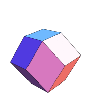
Figure 3. A rhombic dodecahedron

The Voronoi cell of ${\mathcal{F}}(G)$ is a rhombic dodecahedron (shown in Figure 3) with $14$ vertices (in bijection with the strong orientations of $G$), $24$ edges, and $12$ faces (in bijection with the oriented circuits of $G$). All faces are rhombi: each oriented circuit is contained in four different strongly oriented genus-2 subgraphs. Every vertex has valency $3$ or $4$. The orientation $\omega$ of Figure 2 is in fact a strong orientation, and it corresponds to a 4-valent vertex of the Voronoi cell, as there are four $\omega$-compatibly oriented circuits given by

$$C_{1}=e_{3}+e_{4}+e_{7},\qquad C_{2}=e_{5}+e_{6}+e_{7},\qquad C_{3}=e_{1}+e_{2}+e_{3}+e_{4},\qquad C_{4}=e_{1}+e_{2}+e_{5}+e_{6}.$$

An immediate corollary of Theorem 3.1 is the following:

Corollary 3.3.

Let $F$ be a face of ${\mathcal{V}}(G)$ expressed as an intersection

$$F=F_{C_{1}}\cap F_{C_{2}}\cap\dots\cap F_{C_{s}},$$

where $\{F_{C_{i}}:i=1\dots s\}$ are codimension one faces corresponding to oriented circuits $C_{1},C_{2},\dots C_{s}$, respectively. Then the orientations of these circuits are compatible, and the face $F$ corresponds under Amini’s isomorphism to the subgraph $C_{1}\cup C_{2}\cup\dots\cup C_{s}$ with the induced orientation. ∎

This observation lets us choose a better circuit basis: one where the sizes of intersections of pairs of basis circuits are computed by their pairings:

Definition 3.4.

A circuit basis is cancellation-free if, for any pair of basis circuits $C_{i}$ and $C_{j}$, the number of edges in the intersection of the two circuits is computed by their pairing: $|C_{i}\cap C_{j}|=|(C_{i},C_{j})|$.

Note that spanning tree bases are always cancellation-free, as the intersection of any two basis circuits is a simple path. This in particular implies that cancellation-free circuit bases exist for any graph. The following remark shows how to choose a cancellation-free circuit basis based on ${\mathcal{F}}(G)$ alone, without knowledge of $G$ or a spanning tree of $G$.

Remark 3.5.

For any pair of circuits $C_{i}$ and $C_{j}$, there are three possibilities:

1. The orientations of $C_{i}$ and $C_{j}$ are compatible. This is the case if and only if the corresponding faces $F_{C_{i}}$ and $F_{C_{j}}$ intersect.

2. The orientations of $C_{i}$ and $-C_{j}$ are compatible, as in Figure 1 for example. This is the case if and only if $F_{C_{i}}$ and $F_{-C_{j}}$ intersect.

   (Note that for any circuit $C$ and corresponding face $F_{C}$, $F_{-C}=-F_{C}$. Here $-F_{C}$ the face parallel to and geometrically opposite from $F_{C}$. Note also that (1) and (2) co-occur if and only if the circuits $C_{i}$ and $C_{j}$ are edge-disjoint.)

3. Neither of the above is true, that is, $C_{i}$ and $C_{j}$ cannot be compatibly oriented. An example is given by the circuits $C_{1}$ and $C_{2}$ in Figure 4. This is the case if and only if the faces $\{F_{C_{i}},F_{C_{j}},F_{-C_{i}},F_{-C_{j}}\}$ are pairwise disjoint.

In the first two cases $|C_{i}\cap C_{j}|=|(C_{i},C_{j})|$, but not in the third case. Hence, to choose a cancellation-free basis, one only needs to make sure that all pairs of basis circuits are of the first two types, and this can be detected by examining the one-codimension faces of ${\mathcal{V}}(G)$. In Remark 3.15 we will also show how to choose a spanning tree basis, but this takes more work and is not necessary in order to compute ${\mathcal{M}}(G)$.

Figure 4. Two circuits where no compatible orientation is possible.

To continue understanding Theorem 3.1 explicitly, we analyze which set of faces of the Voronoi cell $V(G)$ correspond to a given strongly orientable subgraph $H$ with different strong orientations.

Proposition 3.6.

Let $H$ be a strongly orientable subgraph of $G$. Let $\omega_{H}$ be a strong orientation of $H$ and let $F_{H,\omega_{H}}$ be the face of $V(G)$ corresponding to the pair $(H,\omega_{H})$. Then the set of faces corresponding to $H$ with all of its different strong orientations is the set of faces parallel to, and of the same codimension as $F_{H,\omega_{H}}$.

Proof.

If $F_{H,\omega_{H}}$ is of codimension $s$, then it can be written (not necessarily uniquely) as an intersection $F_{H,\omega_{H}}=F_{C_{1}}\cap\dots\cap F_{C_{s}}$, where $F_{C_{1}},\dots F_{C_{s}}$ are codimension one faces corresponding to oriented circuits $C_{1},\dots C_{s}$. Then, by Corollary 3.3, $H$ can be written as $H=C_{1}\cup\dots\cup C_{s}$. Consider another codimension $s$ face $F^{\prime}$, and write $F^{\prime}=F_{C^{\prime}_{1}}\cap\dots\cap F_{C^{\prime}_{s}}$ as the intersection of $s$ codimension one faces.

The “direction” of $F_{H,\omega_{H}}$ is the orthogonal complementary subspace to the span of the lattice vectors $\{C_{1},\dots,C_{s}\}$, and similarly for $F^{\prime}$. So $F^{\prime}$ and $F$ are parallel if and only if $\text{span}\{C^{\prime}_{1},\dots,C^{\prime}_{s}\}=\text{span}\{C_{1},\dots,C_{s}\}$.

Note that $\text{span}\{C_{1},\dots,C_{s}\}$ is in fact the cycle space of $H$, that is, the subspace of ${\mathcal{F}}(G)\otimes\mathbb{R}$ containing the cycles in $H$ (i.e., the first homology of $H$). Similarly, $\text{span}\{C^{\prime}_{1},\dots,C^{\prime}_{s}\}$ is the cycle space of $H^{\prime}$. Since all components of $H$ and $H^{\prime}$ are two-connected, every edge in $H$ or $H^{\prime}$ participates in a circuit in $H$ or $H^{\prime}$, respectively. Hence, cycle spaces of $H$ and $H^{\prime}$ agree if and only if $H^{\prime}=H$, completing the proof. ∎

3.2. 3-Connected graphs

Our next task is to understand the edges (1-dimensional faces) of the Voronoi cell, which is easily done for 3-connected graphs, and leads to an immediate construction of ${\mathcal{M}}(G)$ in this case. By Amini’s Theorem the edges of ${\mathcal{V}}(G)$ correspond to pairs $(H,\omega_{H})$, where $H$ is a maximal strongly orientable proper subgraph of $G$ and $\omega_{H}$ is a strong orientation of $H$. If $G$ is 3-connected, then for any edge $e\in E(G)$, $G-e$ is 2-connected and hence strongly orientable, and all maximal strongly orientable proper subgraphs are of this form. By Proposition 3.6, there is a parallel class of edges of $V(G)$ corresponding to the subgraph $G-e$ with different strong orientations. This results in the following construction of the graphic matroid ${\mathcal{M}}(G)$ from ${\mathcal{F}}(G)$ for 3-connected graphs $G$.

Theorem 3.7.

Let $G$ be a 3-connected graph with lattice of integer flows ${\mathcal{F}}(G)$, whose Voronoi cell is denoted $V(G)$. Then

1. There is a bijection between $E(G)$ (that is, the ground set of ${\mathcal{M}}(G)$) and the parallel classes of edges of the Voronoi cell $V(G)$.

2. There is a bijection between the circuits of $G$ (that is, the circuits of ${\mathcal{M}}(G)$) and the parallel classes of codimension one faces of $V(G)$.

3. A given edge $e\in E(G)$ belongs to a circuit $C$, that is $C\not\subset G-e$, if and only if no member of the parallel class of edges of $V(G)$ corresponding to $e$ belongs to the face $F_{C}$ (and consequently none of them belong to $F_{-C}$ either).

3.3. 2-Connected graphs

The situation is more complicated when $G$ is not 3-connected. Edges of the Voronoi cell still correspond to pairs $(H,\omega_{H})$, where $H$ is a maximal strongly orientable proper subgraph of $G$. The subgraph $H$ may be of the form $G-e$ for some edge $e$, when $e$ does not participate in a 2-cut and hence $G-e$ is 2-connected, thus strongly orientable.

It is also possible that $H=G-S$, where $S$ is a set of multiple edges: all of these edges must participate in 2-cuts, otherwise $H$ would not be maximal. Note that in this case $H$ has several connected components: indeed, if an edge $e\in S$ participates in a 2-cut $\{e,f\}$ in $g$, then $f$ is a bridge in $G-e$, and so $f\notin H$ as $H$ is strongly orientable.

Constructing ${\mathcal{M}}(G)$ requires understanding the complements $S$ in $E(G)$ of maximal strongly orientable proper subgraphs. They turn out to be what we will call 2-cut blocks, so we begin by defining and describing these.

Lemmas 3.8, 3.10 and  3.11 could be deduced using classical results on minimally 2-connected graphs (see for example [Bol78, Chapter 1.3]), but we choose to prove them directly as the proofs are short and elementary.

Lemma 3.8.

The relation “edges $e$ and $f$ are either the same or form a 2-cut in $G$” is an equivalence relation on $E(G)$.

Proof.

The reflexive and symmetric properties are obvious, so the only point to prove is transitivity. Namely, we need to show that if $\{e,f,h\}$ are three distinct edges of $G$ and $\{e,f\}$ and $\{f,h\}$ are both 2-cuts in $G$ then so is $\{e,h\}$.

Indeed, in the graph $G-f$, the edges $e$ and $h$ are both bridges, so the graph $G-\{e,f,h\}$ has three connected components. Of these three $f$ can only join two, so the graph $G-\{e,h\}$ is still disconnected, meaning that $\{e,h\}$ is a 2-cut. ∎

Definition 3.9.

We call the equivalence classes of the above relation 2-cut blocks in $E(G)$.

Lemma 3.10.

If $S\subset E(G)$, then the subgraph $H=G-S$ is a maximal proper strongly orientable subgraph of $G$ if and only if $S$ is a 2-cut block.

Proof.

Observe that if $H$ is strongly orientable then $S$ is a union of 2-cut blocks. Indeed, if $H$ is strongly orientable then all of its connected components are two-connected, and hence if for some edges $e,f\in E(G)$, $e\in S$ and $\{e,f\}$ is a 2-cut, then it must be that $f\in S$ as well. On the other hand when $S$ is a 2-cut block then $G-S$ is strongly orientable as it contains no bridges: if $e$ is a bridge in $G-S$, then $e$ participates in a 2-cut $\{e,f\}$ in $G$ with $f\in S$, contradicting that $S$ is a 2-cut block. Hence, if $G-S$ is maximal then $S$ is a single 2-cut block and vice versa, as needed. ∎

For each edge $\epsilon$ of the Voronoi cell $V(G)$, let $[\epsilon]$ denote the set of all the edges of $V(G)$ parallel to $\epsilon$, that is, the parallel class of $\epsilon$. By Proposition 3.6, the parallel classes $[\epsilon]$ are in one-to-one correspondence with maximal 2-connected proper subgraphs $H=G-S$, where $S$ is a 2-cut block. Recall that $S$ is a single edge $\{e\}$ if and only if $G-e$ is two-connected, that is if and only if $e$ does not participate in any 2-cuts. Let $S_{[\epsilon]}$ be the 2-cut block corresponding to the parallel class $[\epsilon]$.

The construction of ${\mathcal{M}}(G)$ comes down to detecting the size of $S_{[\epsilon]}$ for each $[\epsilon]$. As in the case of 3-connected graphs in Theorem 3.7, one can then list the circuits of $G$ and tell which 2-cut blocks participate in each circuit based on the poset of faces of $V(G)$. Note that circuits are always unions of entire two-cut blocks, as the following Lemma shows.

Lemma 3.11.

If $S$ is a 2-cut block and $C$ is a circuit in $G$, then either $S$ and $C$ are disjoint or $S\subset C$.

Proof.

Assume that $S\cap C\neq\emptyset$ and let $e\in S\cap C$ be some edge in the intersection. Let $f\in S$ be any other edge in $S$. We need to show that $f\in C$.

Since $f\in S$, we know that $\{e,f\}$ is a 2-cut in $G$, hence $e$ is a bridge in $G-f$, so $e$ does not participate in any circuit in $G-f$. So $C\not\subset(G-f)$, therefore $f\in C$. ∎

Let $n_{[\epsilon]}:=|S_{[\epsilon]}|$ denote the cardinality of the two-cut block $S_{[\epsilon]}$. To finish the construct ${\mathcal{M}}(G)$, we need to compute the numbers $n_{[\epsilon]}$. Let $\mathcal{B}=\{C_{1},...,C_{r}\}$ be a cancellation-free circuit basis of ${\mathcal{F}}(G)$ chosen as in Remark 3.5. For each $S_{[\epsilon]}$ there is some circuit $C_{i}\in\mathcal{B}$ for which $S_{[\epsilon]}\subset C_{i}$. Each $C_{i}\in\mathcal{B}$ corresponds to a codimension one face of $V(G)$, denoted $F_{C_{i}}$. For each $C_{i}\in\mathcal{B}$, the edges of $C_{i}$ can be expressed as a disjoint union of the sets $S_{[\epsilon]}$, where $[\epsilon]$ runs over all edge directions of the Voronoi cell which do not participate in the face $F_{C_{i}}$, as in Theorem 3.7. Hence, for $i=1,\dots,r$ one can write the linear equations

(1) $$\sum_{[\epsilon]\notin F_{C_{i}}}n_{[\epsilon]}=(C_{i},C_{i}),$$

where the notation $[\epsilon]\notin F_{C_{i}}$ means that no edge parallel to $\epsilon$ participates in the face $F_{C_{i}}$. In addition we have a similar linear equation for each pair of circuits $C_{i},C_{j}\in\mathcal{B}$, as the number of edges in $C_{i}\cap C_{j}$ is given by the absolute value of their pairing $|(C_{i},C_{j})|$, as $\mathcal{B}$ is cancellation-free.

(2) $$\sum_{[\epsilon]\notin F_{C_{i}},F_{C_{j}}}n_{[\epsilon]}=|(C_{i},C_{j})|.$$

Note that the resulting system of linear equations always has a positive integer solution, namely, the numbers $n_{[\epsilon]}$ determined by the graph $G$.

Proposition 3.12.

The system (1), (2) has a unique positive integer solution $\{n_{[\epsilon]}\}$.

Proof.

Assume that $\{n_{\epsilon}\}$ is the solution given by the sizes of 2-cut-blocks in $G$, and $\{n^{\prime}_{[\epsilon]}\}$ is a different positive integer solution. Our strategy is to construct a corresponding graph $G^{\prime}$ with 2-cut blocks $S^{\prime}_{[\epsilon]}$ of sizes $n^{\prime}_{[\epsilon]}$, and show that $G$ and $G^{\prime}$ are 2-isomorphic.

The edges of $G$ are paritioned by the sets $S_{[\epsilon]}$, with $|S_{[\epsilon]}|=n_{[\epsilon]}$. Assume that for some $\epsilon$, $n^{\prime}_{[\epsilon]}>n_{[\epsilon]}$. Choose an arbitrary edge of $S_{[\epsilon]}$ and split it into $n^{\prime}_{[\epsilon]}-n_{[\epsilon]}+1$ edges by creating $n^{\prime}_{[\epsilon]}-n_{[\epsilon]}$ degree two vertices on it, preserving the edge orientation. Call the resulting graph $G^{*}$, and the changed 2-cut block $S^{*}_{[\epsilon]}$. First, note that in $G^{*}$, $S^{*}_{[\epsilon]}$ is a in fact 2-cut block, that is, any two of its edges form a 2-cut. Furthermore, $|S^{*}_{[\epsilon]}|=n^{\prime}_{[\epsilon]}$, and all other 2-cut blocks are unchanged. In addition, the circuits of $G$ are in bijection with the circuits of $G^{*}$, in the obvious way, and linear independence of circuits is preserved. (Informally speaking, the edge splitting operation does not change the cycle structure of $G$ except for the lengths of cycles.)

On the other hand, if for some $\epsilon$, $n^{\prime}_{[\epsilon]}<n_{[\epsilon]}$, then choose $n_{[\epsilon]}-n^{\prime}_{[\epsilon]}$ arbitrary edges of $S_{[\epsilon]}$ and contract them. Again call the resulting graph $G^{*}$, and note that the newly created $S^{*}_{[\epsilon]}$ is a 2-cut block in $G^{*}$ of cardinality $n^{\prime}_{[\epsilon]}$, while all other 2-cut blocks are unchanged.

This operation also preserves the circuits of $G$: first note that any circuit in $G$ which intersects with $S_{[\epsilon]}$ contains it, and $n^{\prime}_{[\epsilon]}$ is still a positive integer, so circuits are never contracted to nothing. Furthermore, circuits remain circuits: only edges that participate in 2-cuts are ever contracted and hence, if a closed walk didn’t repeat vertices in $G$, it still does not do so in $G^{*}$. Finally, the edge contractions do not create new circuits: if a closed walk in $G$ repeats a vertex, it will still do so in $G^{*}$. In summary, the circuits of $G$ are in bijection with the circuits of $G^{*}$. Linear independence of circuits is also preserved.

Now carry out this process for all $[\epsilon]$ to create a new graph $G^{\prime}$ with 2-cut blocks $S^{\prime}_{[\epsilon]}$ of sizes $n^{\prime}_{[\epsilon]}$. We claim that ${\mathcal{F}}(G)\cong{\mathcal{F}}(G^{\prime})$. Recall that $\{C_{1},\dots,C_{r}\}$ is a circuit basis for ${\mathcal{F}}(G)$, and call the gram matrix corresponding to this circuit basis $M$. Let $\{C^{\prime}_{1},\dots,C^{\prime}_{r}\}$ be the circuits in $G^{\prime}$ created from $\{C_{1},\dots,C_{r}\}$, respectively. Since circuits and linear independence were preserved, these form a circuit basis for ${\mathcal{F}}(G^{\prime})$; let us call the corresponding Gram matrix $M^{\prime}$.

Since the $C_{i}$ form a cancellation-free basis of ${\mathcal{F}}(G)$, the entries of the absolute value $|M|$ are the sizes of intersections $|C_{i}\cap C_{j}|$, with $i,j=1...r$. The basis $\{C_{1}^{\prime},...,C_{r}^{\prime}\}$ is also cancellation-free: the characterization of Remark 3.5 shows that the edge splittings and contractions do not change this property. Since the $\{n_{\epsilon}\}$ and $\{n^{\prime}_{[\epsilon]}\}$ are both solutions to the system of equations (1) and (2), we deduce that $|M|=|M^{\prime}|$.

Furthermore, the sign of the $(i,j)$ entry of $M$ depends on whether $C_{i}$ and $C_{j}$ are oriented compatibly or opposite (where opposite means that the orientation of $C_{i}$ is compatible with that of $-C_{j}$). This is unchanged by edge splittings and contractions, hence the sign of each entry is the same in $M$ and $M^{\prime}$. So $M=M^{\prime}$ and ${\mathcal{F}}(G)\cong{\mathcal{F}}(G^{\prime})$. Thus, by Theorem 2.1, this lifts to an isomorphism $\mathbb{Z}^{E(G)}\to\mathbb{Z}^{E(G^{\prime})}$, which sends each edge of $G$ to a signed edge of $G^{\prime}$, creating edge bijections within the 2-cut blocks. So $n_{\epsilon}=n^{\prime}_{\epsilon}$ for all $\epsilon$ as needed. ∎

Theorem 3.13.

The graphic matroid ${\mathcal{M}}(G)$ of a 2-connected graph $G$ can be computed explicitly from the lattice of integer flows ${\mathcal{F}}(G)$ by the following algorithm:

1. List the one-codimensional faces of the Voronoi cell $V(G)$ of ${\mathcal{F}}(G)$, and use this to choose a good circuit basis $\{C_{1},...,C_{r}\}$ for ${\mathcal{F}}(G)$ as explained in Remark 3.5.

2. List the edges $\{\epsilon\}$ of $V(G)$, and group them into parallel classes $\{[\epsilon]\}$. For each circuit $C$, list which edge directions participate in the face $F_{C}$.

3. For each basis circuit $C_{i},i=1...r$, write the equation

   $$\sum_{[\epsilon]\notin F_{C_{i}}}n_{[\epsilon]}=(C_{i},C_{i}),$$

   and for each pair of basis circuits $\{\{F_{C_{i}},F_{C_{j}}\},i,j=1...r,i\neq j\}$ write the equation

   $$\sum_{[\epsilon]\notin F_{C_{i}},F_{C_{j}}}n_{[\epsilon]}=(C_{i},C_{j}).$$

4. Solve the system of linear equations, to find the unique positive integer solution $\{n_{[\epsilon]}\}$.

5. The ground set of ${\mathcal{M}}(G)$ is the edge set $E(G)$, which can be written as a disjoint union of the sets $\{S_{[\epsilon]}\}$ whose sizes are given by the solution $\{n_{[\epsilon]}\}$.

6. The edge $e$ belongs to a circuit $C$ if and only if no member of the corresponding edge parallel class $[\epsilon]$ in $V(G)$ belongs to the face $F_{C}$.

Example 3.14.

As an example, let us carry out the algorithm for the graph of Example 3.2, and construct the graphic matroid ${\mathcal{M}}(G)$ from ${\mathcal{F}}(G)$.

1. We start with the Gram matrix of ${\mathcal{F}}(G)$ given by

   $$\begin{pmatrix}3&1&2\\ 1&3&0\\ 2&0&4\end{pmatrix}.$$

   (This is the Gram matrix with respect to the circuit basis in Example 3.2.) We compute the Voronoi cell $V(G)$ of ${\mathcal{F}}(G)$ which is the rhombic dodecahedron shown in Figure 3. It has 12 faces. Of these we choose three pairwise intersecting ones, thus forming a cancellation-free basis: let $F_{C_{1}}$ be the top right (white) face of the dodecahedron shown in Figure 3, $F_{C_{2}}$ the top (light blue) face, and $F_{C_{3}}$ the front (light purple) face.

2. The rhombic dodecahedron has 24 edges belonging to four parallel classes (of 6 edges each). Let $\epsilon_{1}$ be the edge between the two left side faces (dark blue and dark purple), $\epsilon_{2}$ the edge between the two right side faces (white and orange), $\epsilon_{3}$ be the edge between the front and top left faces (light purple and dark blue), and $\epsilon_{4}$ the edge between the front and top right faces (light purple and white).

   The parallel classes $\{[\epsilon_{2}],[\epsilon_{4}]\}$ appear in $F_{C_{1}}$, $\{[\epsilon_{1}],[\epsilon_{2}]\}$ appear in $F_{C_{2}}$, and $\{[\epsilon_{3}],[\epsilon_{4}]\}$ appear in $F_{C_{3}}$.

3. $n_{1}+n_{3}=3,\quad n_{3}+n_{4}=3,\quad n_{1}+n_{2}=4,\quad n_{3}=1,\quad n_{1}=2,\quad 0=0$.

4. $n_{1}=2,\quad n_{2}=2,\quad n_{3}=1,\quad n_{4}=2$.

5. There are 7 edges partitioned into sets $E(G)=\bigcup_{i=1}^{4}S_{i}$ with $|S_{i}|=n_{i}$.

6. There are six (unoriented) circuits corresponding to parallel pairs of faces of $V(G)$. These are: $C_{1}$, $C_{2}$, $C_{3}$, $C_{4}=C_{3}+C_{2}-C_{1}$, $C_{5}=C_{1}-C_{2}$, and $C_{6}=C_{3}-C_{1}$. They can be expressed in terms of the $S_{i}$ as follows: $C_{1}=S_{[\epsilon_{1}]}\cup S_{[\epsilon_{3}]}$, $C_{2}=S_{[\epsilon_{3}]}\cup S_{[\epsilon_{4}]}$, $C_{3}=S_{[\epsilon_{1}]}\cup S_{[\epsilon_{2}]}$, $C_{4}=S_{[\epsilon_{2}]}\cup S_{[\epsilon_{4}]}$, $C_{5}=S_{[\epsilon_{1}]}\cup S_{[\epsilon_{4}]}$, and $C_{6}=S_{[\epsilon_{2}]}\cup S_{[\epsilon_{3}]}$. In other words, ${\mathcal{M}}(G)$ is given by the $(0,1)$-matrix

   (3) $$\begin{bmatrix}1&1&0&0&1&0&0\\ 0&0&0&0&1&1&1\\ 1&1&1&1&0&0&0\\ 0&0&1&1&0&1&1\\ 1&1&0&0&0&1&1\\ 0&0&1&1&1&0&0\\ \end{bmatrix}$$

In Figure 2, we see a representative $G$ of the 2-isomorphism class of graphs given by ${\mathcal{F}}(G)$. In this representative, $S_{[\epsilon_{1}]}=\{e_{3},e_{4}\}$, $S_{[\epsilon_{2}]}=\{e_{1},e_{2}\}$, $S_{[\epsilon_{3}]}=\{e_{7}\}$, and $S_{[\epsilon_{4}]}=\{e_{5},e_{6}\}$.

Remark 3.15.

In [SW10] Su and Wagner prove that the lattice of integer flows ${\mathcal{F}}(M)$ of a regular matroid $M$ determines the matroid up to co-loops. Their proof is almost constructive, but requires the input of a “fundamental basis of ${\mathcal{F}}(M)$ coordinatized by a basis of $M$”. In the context of graphic matroids (which form a sub-class of regular matroids) this means the input of a spanning-tree basis, that is, the set of fundamental circuits corresponding to some spanning tree of $G$, as described in Section 2. As a final remark we show how to choose a spanning-tree basis for ${\mathcal{F}}(G)$, making the proof in [SW10] fully constructive for graphic matroids.

To choose a spanning-tree basis, the first step is the same as before: list the one codimension faces and parallel classes of edges of $V(G)$. Then construct a 0-1 matrix, the rows of which are indexed by the (unoriented) circuits of $G$ and the columns by the 2-cut blocks $S_{[\epsilon]}$ as follows. Place a $1$ in the field $(C,S_{[\epsilon]})$ if and only if $S_{[\epsilon]}\subset C$, which is the case if and only if $[\epsilon]\notin F_{C}$.

A spanning-tree basis of $G$ can be found by the following greedy algorithm. To find a spanning tree, one needs to delete edges from a graph until no circuits remain, but so that the graph stays connected. Consider the first row of the matrix, indexed by the circuit $C_{1}$. Find the first $1$ in the row $C_{1}$, without loss of generality assume that $S_{1}\subset C_{1}$. Imagine deleting (we say imagine, as $G$ is not known to us) one edge from $S_{1}$, thereby breaking the circuit $C_{1}$. To mark this change, turn all the $1$’s in the column of $S_{1}$ red: all the circuits which contained $S_{1}$ are now broken.

Now find the first unbroken circuit (i.e. one which has no red $1$ in its row). Delete (in the “imaginary” graph $G$) one edge of the first 2-cut block which participates in it, and turn all the $1$’s in that column red. Continue in this manner until no circuits are left intact, i.e. until every row has a red $1$ in it.

The process will clearly terminate. At the end we know that there are no circuits left in $G$, although we don’t know $G$. Also, $G$ remains connected as only edges which participate in a circuit are ever deleted. Hence, what remains is a spanning tree of $G$. The elements of the corresponding spanning-tree basis of ${\mathcal{F}}(G)$ are those circuits which have exactly one edge not in the spanning tree, i.e., the circuits which have only one red $1$ in their row at the end of the algorithm.

As an illustration, applying the above algorithm to the lattice of integer flows in Example 3.14, we obtain the matrix

$$\begin{bmatrix}1&0&1&0\\ 0&0&1&1\\ 1&1&0&0\\ 0&1&0&1\\ 1&0&0&1\\ 0&1&1&0\\ \end{bmatrix}$$

This is the same matrix as (3), except with only one column for each two-cut block $S_{\epsilon}$, and we don’t need to know what the sizes of the blocks are. Carrying out the algorithm leads to the following matrix (marking red 1’s by $*$ for black and white print):

$$\begin{bmatrix}{\color[rgb]{1.00,0.00,0.00}1*}&0&{\color[rgb]{1.00,0.00,0.00}1*}&0\\ 0&0&{\color[rgb]{1.00,0.00,0.00}1*}&1\\ {\color[rgb]{1.00,0.00,0.00}1*}&{\color[rgb]{1.00,0.00,0.00}1*}&0&0\\ 0&{\color[rgb]{1.00,0.00,0.00}1*}&0&1\\ {\color[rgb]{1.00,0.00,0.00}1*}&0&0&1\\ 0&{\color[rgb]{1.00,0.00,0.00}1*}&{\color[rgb]{1.00,0.00,0.00}1*}&0\\ \end{bmatrix}$$

From this we read off the spanning tree basis $\{C_{2},C_{4},C_{5}\}$. This basis corresponds to the spanning tree $\{e_{2},e_{4},e_{5},e_{6}\}$ with the notation of Figure 2, though the algorithm does not output this information.

Acknowledgment

The authors wish to thank Dror Bar-Natan, Josh Greene, Tony Licata, and Brendan McKay for useful conversations. S.G. was supported in part by in part by the National Science Foundation Grant DMS-14-06419.

References

- [Ami10] Omid Amini, Lattice of Integer Flows and Poset of Strongly Connected Orientations, 2010, arXiv:1007.2456, Preprint.
- [Art06] I. V. Artamkin, The discrete Torelli theorem, Mat. Sb. 197 (2006), no. 8, 3–16.
- [BdlHN97] Roland Bacher, Pierre de la Harpe, and Tatiana Nagnibeda, The lattice of integral flows and the lattice of integral cuts on a finite graph, Bull. Soc. Math. France 125 (1997), no. 2, 167–198.
- [Bol78] Béla Bollobás, Extremal graph theory, London Mathematical Society Monographs, vol. 11, Academic Press, Inc. [Harcourt Brace Jovanovich, Publishers], London-New York, 1978.
- [BW88] Robert E. Bixby and Donald K. Wagner, An almost linear-time algorithm for graph realization, Math. Oper. Res. 13 (1988), no. 1, 99–123.
- [CV10] Lucia Caporaso and Filippo Viviani, Torelli theorem for graphs and tropical curves, Duke Math. J. 153 (2010), no. 1, 129–171.
- [Fuj80] Satoru Fujishige, An efficient PQ-graph algorithm for solving the graph-realization problem, J. Comput. System Sci. 21 (1980), no. 1, 63–86.
- [Gre13] Joshua E. Greene, Lattices, graphs, and Conway mutation, Invent. Math. 192 (2013), no. 3, 717–750.
- [GY06] Jonathan L. Gross and Jay Yellen, Graph theory and its applications, second ed., Discrete Mathematics and its Applications (Boca Raton), Chapman & Hall/CRC, Boca Raton, FL, 2006.
- [OS79] Tadao Oda and C. S. Seshadri, Compactifications of the generalized jacobian variety, Trans. Amer. Math. Soc. 253 (1979), 1–90.
- [Oxl92] James G. Oxley, Matroid theory, Oxford Science Publications, The Clarendon Press, Oxford University Press, New York, 1992.
- [SW10] Yi Su and David G. Wagner, The lattice of integer flows of a regular matroid, J. Combin. Theory Ser. B 100 (2010), no. 6, 691–703.
- [Wag98] David G. Wagner, The algebra of flows in graphs, Adv. in Appl. Math. 21 (1998), no. 4, 644–684.
- [Whi33] Hassler Whitney, 2-Isomorphic Graphs, Amer. J. Math. 55 (1933), no. 1-4, 245–254.