Properties of frequentist confidence levels derivatives

Abstract

In high energy physics, results from searches for new particles or rare processes are often reported using a modified frequentist approach, known as $\rm{CL_{s}}$ method. In this paper, we study the properties of the derivatives of $\rm{CL_{s}}$ and $\rm{CL_{s+b}}$ as signal strength estimators if the confidence levels are interpreted as credible intervals. Our approach allows obtaining best fit points and $\chi^{2}$ functions which can be used for phenomenology studies. In addition, this approach can be used to incorporate $\rm{CL_{s}}$ results into Bayesian combinations.

1 Introduction

A method that is commonly used in high energy physics to set limits in production cross sections of hypothetical new particles [1] as well as in branching fractions of rare decay processes (e.g. [2, 3]), is the so-called $\textrm{CL}_{\textrm{s}}$ method, or modified frequentist approach [4, 5] . This approach has become very popular because it avoids unphysical limits as well as the possibility of setting strong limits in experiments with no sensitivity. However, it does not reveal other potentially relevant information, as for example what is the most probable value for the signal cross section. To construct a likelihood function or a probability density function ($p.d.f.$, $\rm P(s|data)$) out of these results, sometimes a Gaussian approach is used. In the Gaussian approach the $90\%~{}(95\%)$ one-sided limits are converted to 1.6 (2) standard deviations. However this is in general a very rough approach.

In this paper, we describe a series of methods to obtain posterior probabilities from published $\textrm{CL}_{\textrm{s}}(s)$ and $\textrm{CL}_{\textrm{s+b}}(s)$ curves. These approaches were used for implementing constraints in the phenomenological analyses of Ref. [7, 8], as well as to crosscheck the coverage of upper limits based on profile likelihood integration. The posterior probabilities obtained through these methods can be folded as prior probabilities for Bayesian combinations with other results.

2 Mathematical definitions

Our goal is to obtain a $p.d.f.$ for the signal strength such that the credible intervals obtained with this function match the frequentist confidence levels $\textrm{CL}_{\textrm{s+b}}$ or the confidence level ratio $\textrm{CL}_{\textrm{s}}$ given by an experiment. Hereafter we restrict ourselves to a single signal-strength parameter $s$. The quantities $\textrm{CL}_{\textrm{s+b}}$ and $\textrm{CL}_{\textrm{s}}$ are assumed to be monotonically decreasing with $s$, as expected from any routine meant to set upper limits. Continuity and differentiability are desired, although not strict requirements since in practice the derivatives will be approximated numerically. Because the credible interval (or Bayesian confidence level) is the integral of the $p.d.f.$, the quantity:

$$\delta(s)\equiv-\frac{d\textrm{CL}_{\textrm{s+b}}}{ds}\quad,$$ (1)

where $s$ represents the signal strength, gives us a $p.d.f.$ with credible intervals that are equivalent to the frequentist $\textrm{CL}_{\textrm{s+b}}$ and that therefore has by construction the appropriate coverage:

$$\textrm{CL}_{\textrm{s+b}}(\sigma)=\int_{-\sigma_{min}}^{\sigma}\delta(s)ds$$ (2)

where $\sigma_{min}$ is the minimum value of the signal strenght (including negative values) which is still consistent with non-negative entries in all the bins, so that Poisson statistics still applies. Arbitrary integration constants have been omitted.

However, upper limits are commonly set using $\textrm{CL}_{\textrm{s}}$ and not $\textrm{CL}_{\textrm{s+b}}$. On one hand, this sacrifices part of the coverage, but on the other hand avoids excluding the null hypothesis as well as obtaining strong limits in experiments with no sensitivity. Therefore we define the quantity:

$$\phi(s)\equiv-\frac{d\textrm{CL}_{\textrm{s}}}{ds}$$ (3)

to provide the $p.d.f.$ with credible intervals equivalent to $\textrm{CL}_{\textrm{s}}$ limits:

$$\textrm{CL}_{\textrm{s}}(\sigma)=\int_{0}^{\sigma}\phi(s)ds\quad.$$ (4)

In the particular case of a single bin analysis and without systematic uncertainties, $\phi(s)$ is equivalent to a posterior built from the likelihood function multiplied by a constant positive $s$ prior [5]. Normalization constants should be set such that $\delta(s)$ and $\phi(s)$ integrate to unity over the s domain.

The function $\delta(s)$ is closely related to the likelihood function. Indeed, as discussed in Appendix 7 of [9], Bayesian credible intervals have the frequentist coverage averaged with respect to the prior density. As $\delta(s)$ has by construction the frequentist coverage, it is expected that the corresponding prior that weighs the coverage is constant or nearly constant in the entire phase space. However, note that $\delta(s)$ can differ from the profile likelihood, due to the fact that credible integrals of the latter do not always have the required coverage, while credible intervals of $\delta(s)$ do.

In the case of a single bin experiment it is easy to demonstrate that $\delta(s)$ corresponds to the likelihood function. Since the following relation holds

$$-\frac{d\textrm{CL}_{\textrm{s+b}}}{ds}=-\sum_{N=0}^{N_{obs}}\frac{df(s,N)}{ds}\quad,$$ (5)

where $N$ is the number of events and $f(s,N)$ is the two-dimensional distribution of the possible outcomes of the test-statistic in the $s,N$ plane, given by Poisson statistics as

$$f(s,N)=\frac{(s+b)^{N}e^{-(s+b)}}{N!}\quad,$$ (6)

then

$$\delta(s)_{count} = -\frac{d\textrm{CL}_{\textrm{s+b}}}{ds}_{count}=-\sum_{N=0}^{N_{obs}}\frac{df(s,N)}{ds}=$$

$$= \sum_{N=0}^{N_{obs}}\left(\frac{(s+b)^{N}e^{-(s+b)}}{N!}-\frac{N(s+b)^{N-1}e^{-(s+b)}}{N!}\right)$$

$$= \frac{(s+b)^{N_{obs}}e^{-(s+b)}}{N_{obs}!}=f(N_{obs}|s)_{count}\quad.$$

One property of $\delta(s)$, independent of the choice of test-statistic, is such that if multiplied by a constant positive $s$ prior $\theta(s)$ one finds that:

$$\frac{\mathop{\text{\Large$\int_{\text{\normalsize$\scriptstyle\kern-1.39998pt-\infty$}}^{\text{\normalsize$\scriptstyle\sigma$}}$}}\nolimits\theta(s)\delta(s)ds}{\mathop{\text{\Large$\int_{\text{\normalsize$\scriptstyle\kern-1.39998pt-\infty$}}^{\text{\normalsize$\scriptstyle+\infty$}}$}}\nolimits\theta(s)\delta(s)ds}=\frac{\mathop{\text{\Large$\int_{\text{\normalsize$\scriptstyle\kern-1.39998pt\lim_{s\rightarrow 0}s$}}^{\text{\normalsize$\scriptstyle\sigma$}}$}}\nolimits\delta(s)ds}{\mathop{\text{\Large$\int_{\text{\normalsize$\scriptstyle\kern-1.39998pt\lim_{s\rightarrow 0}s$}}^{\text{\normalsize$\scriptstyle+\infty$}}$}}\nolimits\delta(s)ds}=\frac{\lim_{s\rightarrow 0}\textrm{CL}_{\textrm{s+b}}(s)-\textrm{CL}_{\textrm{s+b}}(\sigma)}{\lim_{s\rightarrow 0}\textrm{CL}_{\textrm{s+b}}(s)-0}=\\ =\frac{\lim_{s\rightarrow 0}\textrm{CL}_{\textrm{b}}(s)-\textrm{CL}_{\textrm{s+b}}(\sigma)}{\lim_{s\rightarrow 0}\textrm{CL}_{\textrm{b}}(s)}\approx 1-\textrm{CL}_{\textrm{s}}(\sigma)$$ (8)

i.e. upper limits derived from the integration of $\delta(s)$ on the positive range of $s$ are expected to be very close to those obtained from $\textrm{CL}_{\textrm{s}}$. The above approximation is exact in the case where $\textrm{CL}_{\textrm{b}}$ is independent of $s$, which is possible for certain choices of the test-statistic. In these cases, $\theta(s)\delta(s)=\phi(s)$. This interesting relation leads us to define:

$$\epsilon(s)=\frac{\phi(s)}{\delta(s)}$$ (9)

which can be understood as the effective prior on $s$ needed to get limits equivalent to $\textrm{CL}_{\textrm{s}}$.

It can also be noticed that:

$$1-\int_{0}^{+\infty}\delta(s)ds=1-\lim_{s\rightarrow 0}\textrm{CL}_{\textrm{b}}(s)$$ (10)

which can be used to build background-only $p$-values. This is interesting as from a combination of null searches, with only upper limits, a non-null combination could also be derived. In particular, for a test-statistic in which $\textrm{CL}_{\textrm{b}}$ does not depend on $s$, the usual $p$-value used in $\textrm{CL}_{\textrm{s}}$ should be identical to what is obtained from Eq. (10). On the contrary, $\phi(s)$ is by construction normalized to 1 in the positive range of $s$. When $\phi$ or $\delta$ are interpreted as probabilities, one can build a $\chi^{2}$ function out of them as:

$$\chi^{2}_{\delta}(s) = -2\log{\frac{\delta(s)}{max\left\{\delta(s)\right\}}}$$ (11)

$$\chi^{2}_{\phi}(s) = -2\log{\frac{\phi(s)}{max\left\{\phi(s)\right\}}}\quad.$$ (12)

3 Numerical tests and examples

In this section we demonstrate few examples of $\delta(s)$, $\phi(s)$ and $\epsilon(s)$ functions as obtained from certain hypothetical experiments.

3.1 Classic case

We start by showing examples on how $\delta(s)$, $\phi(s)$ and $\varepsilon(s)$ behave when no systematic uncertainties are included. A typical test-statistic used in the $\textrm{CL}_{\textrm{s}}$ method is:

$$Q=\prod_{i}\frac{e^{-(s_{i}+b_{i})}(s_{i}+b_{i})^{d_{i}}/d_{i}!}{e^{-(b_{i})}(b_{i})^{d_{i}}/d_{i}!}$$ (13)

where $s_{i}$ and $b_{i}$ represent the number of expected signal and background events in the i-th bin, respectively, and $d_{i}$ refers to the number of observed events in the same bin. We use the mc_limit package [10] for calculating $\textrm{CL}_{\textrm{s}}$ and $\textrm{CL}_{\textrm{s+b}}$ in the examples of this subsection.

In our tests, we calculate the derivatives in a numeric way to obtain $\delta$ and $\phi$. In order to get a smooth lineshape for $\delta(s)$ one needs to run a large amount of toy experiments, to generate values of $\textrm{CL}_{\textrm{s+b}}$ with enough digits. Fig. 1 shows both $\textrm{CL}_{\textrm{s}}$ and $\textrm{CL}_{\textrm{s+b}}$ as a function of the signal strength for a single bin experiment, with a background expectation of 0.5 events, a signal expectation varying between 0 and 5 events, and an observation of one event. For each value of $s$, $f(N_{obs}|s)_{count}$ is shown, and compared to the $\delta(s)$ and $\phi(s)$ functions calculated using 20k, 200k and 600k pseudo-experiments (Fig. 2). The ratio between $\phi$ and $\delta$, $\varepsilon(s)$, is computed and shown for the different sets of pseudo-experiments (Fig. 3). It can be seen that a large number of pseudo-experiments is needed in order to properly recover the shape of $\delta$, $\phi$, and $\varepsilon$.

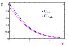
Figure 1: $\textrm{CL}_{\textrm{s}}$ (blue circles) and $\textrm{CL}_{\textrm{s+b}}$ (magenta squares) as a function of the signal expectation, $\left\langle s\right\rangle$, calculated using 600k toy experiments.

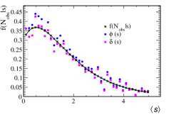
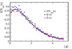
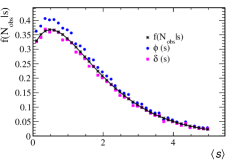
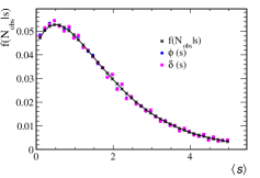
Figure 2: $f(N_{obs}|s)_{count}$ (black solid line), $\delta(s)$ (blue circles), and $\phi(s)$ (magenta squares) calculated using 20k (upper left), 200k (upper right) and 600k (bottom left) toy experiments. The plot on the bottom right shows the same curves as in bottom left, but all normalized to have the same area (i.e, normalized in the $s>0$ range).

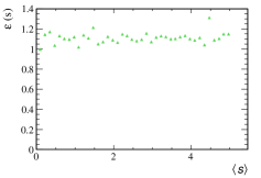
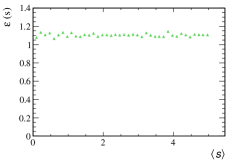
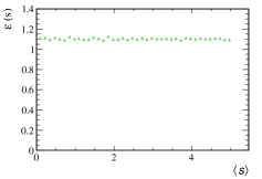
Figure 3: $\varepsilon(s)$ for 20k (upper left), 200k (upper right) and 600k (center) toy experiments.

3.2 Difference between two fits as test-statistic

In this example we will explore the use of a test-statistic constructed as the likelihood ratio between the background hypothesis and the best fit point for $s$, hereafter $\hat{s}$:

$$R=\prod_{i}\frac{e^{-(\hat{s}f_{i}+b_{i})}(\hat{s}f_{i}+b_{i})^{d_{i}}/d_{i}!}{e^{-(b_{i})}(b_{i})^{d_{i}}/d_{i}!}$$ (14)

where $f_{i}$ is the signal fraction in the $i$-th bin, so that $\Sigma f_{i}=1$. The test statistic $R$ is independent of the signal hypothesis and so it will be $\textrm{CL}_{\textrm{b}}$. Therefore, in this case Eq. (8) should hold exactly. As a numerical example we will use a search experiment of a gaussian signal in the mass spectrum, on top of an exponential background. The mass range is [5309.6, 5429.6] ${\mathrm{\,Me\kern-1.00006ptV\!/}c^{2}}$, and the mass peak is at 5369.6 ${\mathrm{\,Me\kern-1.00006ptV\!/}c^{2}}$ with a resolution of 22 ${\mathrm{\,Me\kern-1.00006ptV\!/}c^{2}}$. The background slope is assumed to be $-10^{-4}/({\mathrm{\,Me\kern-1.00006ptV\!/}c^{2}})$. In Fig. 4 we show the mass distribution of the generated data, superimposed with the best fit. In Table 1 we show the 90 and 95% upper limits from $\textrm{CL}_{\textrm{s}}$ and $\textrm{CL}_{\textrm{s+b}}$ obtained from those curves, using both R and Q as test-statistics.

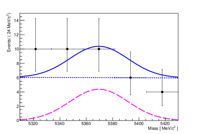
Figure 4: Mass distribution of the generated data for the experiments with (Sect. 3.3) and without (Sect. 3.2) systematic uncertainties. The magenta dashed line shows the signal contribution, the dotted blue line the background, and the solid blue line the total model.

Table 1: 90% and 95% upper limits on $s$ as obtained with different estimators and test statistics (See text for details).

Confidence Level	Estimator and test statistic	Excluded $s$
90%	$\textrm{CL}_{\textrm{s}}^{Q}$,$\textrm{CL}_{\textrm{s}}^{R}$	16.9, 17.0
90%	$\textrm{CL}_{\textrm{s+b}}^{Q}$,$\textrm{CL}_{\textrm{s+b}}^{R}$	16.8, 16.8
95%	$\textrm{CL}_{\textrm{s}}^{Q}$,$\textrm{CL}_{\textrm{s}}^{R}$	19.3, 19.3
95%	$\textrm{CL}_{\textrm{s+b}}^{Q}$,$\textrm{CL}_{\textrm{s+b}}^{R}$	19.2, 19.1

In Fig. 5 we show the $\delta(s)$, $\phi(s)$ and $\epsilon(s)$ curves obtained for the two choices of test-statistic, and compared with the likelihood scan from a fit to the data, as well as with the Markov Chain Monte Carlo posterior mcmc1 obtained from mc_limit [10]. It can be seen that $\delta(s)$ is very similar to the likelihood function, and $\phi(s)$ to the likelihood multiplied by a flat $s>0$ prior.

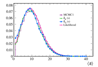
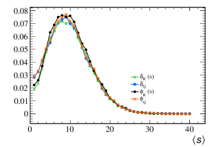
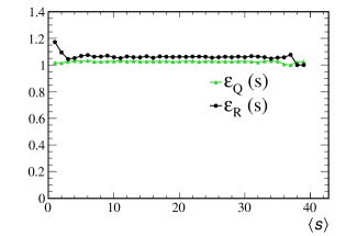
Figure 5: Top: mcmc1 posterior from mc_limit (violet solid line), $\delta_{R}(s)$ (green triangles), $\delta_{Q}(s)$ (cyan squares), likelihood (pink stars). Medium: $\delta_{R}(s)$ (green triangles), $\delta_{Q}(s)$ (cyan squares), $\phi_{R}(s)$ (black circles), $\phi_{Q}(s)$ (orange asterisks). Bottom: $\varepsilon_{Q}(s)$ (green triangles), $\varepsilon_{R}(s)$ (black circles). Experiment with no systematics (Sect. 3.2).

3.3 Fit with systematic uncertainties

In the following example we will use a search experiment of a gaussian signal in the mass spectrum, on top of an exponential background, as it is done in Sect. 3.2, but in the presence of the following nuisance parameters:

• $N_{b}$, the expected number of background events, which is approximately known from an external source.

• $\kappa$, the coefficient of the exponential mass $p.d.f.$ of the background.

• $M$, the peak position.

• $\sigma$, the invariant mass resolution.

All these parameters are considered to have gaussian errors. The test statistic will be the difference in the log-likelihood between a fit with the signal strength set to zero and a fit with the signal strength free. The nuisance parameters are fitted taking into account their prior constraints. The ensembles of pseudo-experiments are generated fluctuating the nuisance parameters according to their prior probabilities. In Fig. 6 we compare the $\textrm{CL}_{\textrm{s+b}}$ and $\textrm{CL}_{\textrm{b}}$ curves obtained using $Q$ and $R$ test-statistics. We see that, as expected, $\textrm{CL}_{\textrm{b}}^{R}$ is independent of $s$, which is not the case of $\textrm{CL}_{\textrm{b}}^{Q}$. This is a very useful property, since otherwise one has to make a choice of $s$ in a somewhat arbitrary manner in order to report a background $p$-value. In Fig. 7 we show $\delta(s)$, $\phi(s)$ and $\epsilon(s)$ using the nuisance parameter values as listed in Table 2.

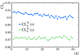
Figure 6: $\textrm{CL}_{\textrm{b}}^{Q}$ (cyan squares) and $\textrm{CL}_{\textrm{b}}^{R}$ (green triangles) as a function of the signal expectation, $\left\langle s\right\rangle$. Experiment with no systematics (Sect. 3.2).

Table 2: Nuisance parameter values for the numeric example

Nuisance Parameter	value
$\kappa$	$(-1.0\pm 0.3)\times 10^{-4}({\mathrm{\,Me\kern-1.00006ptV\!/}c^{2}})^{-1}$
$M$	$5369.6\pm 1{\mathrm{\,Me\kern-1.00006ptV\!/}c^{2}}$
$\sigma$	$22\pm 2{\mathrm{\,Me\kern-1.00006ptV\!/}c^{2}}$
$N_{b}$	$30_{-5}^{+15}$

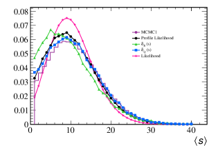
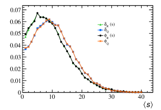
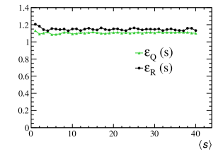
Figure 7: Top: MCM1 (violet solid line), profile likelihood (black circles), $\delta_{R}(s)$ (green triangles), $\delta_{Q}(s)$ (cyan squares), likelihood (pink stars). Medium: $\delta_{R}(s)$ (green triangles), $\delta_{Q}(s)$ (cyan squares), $\phi_{R}(s)$ (black circles), $\phi_{Q}(s)$ (orange asterisks). Bottom: $\varepsilon_{Q}(s)$ (green triangles), $\varepsilon_{R}(s)$ (black circles). Experiment with systematics (Sect. 3.3), where $N_{obs}>\left\langle b\right\rangle$.

An example where the number of observed events is less than the one predicted with the null hypothesis is also performed, leading to the $\delta(s)$, $\phi(s)$ and $\epsilon(s)$ of Fig. 8. In Fig. 9 we show the mass distribution of the generated data.

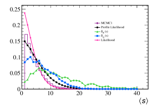
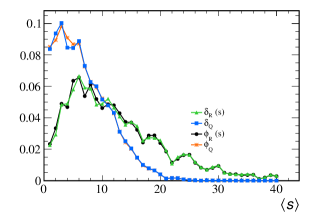
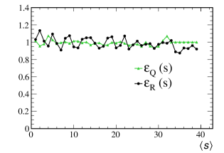
Figure 8: Top: MCM1 (violet solid line), profile likelihood (black circles), $\delta_{R}(s)$ (green triangles), $\delta_{Q}(s)$ (cyan squares), likelihood (pink stars). Medium: $\delta_{R}(s)$ (green triangles), $\delta_{Q}(s)$ (cyan squares), $\phi_{R}(s)$ (black circles), $\phi_{Q}(s)$ (orange asterisks). Bottom: $\varepsilon_{Q}(s)$ (green triangles), $\varepsilon_{R}(s)$ (black circles). Experiment with systematics (Sect. 3.3), where $N_{obs}<\left\langle b\right\rangle$.

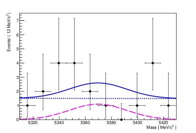
Figure 9: Mass distribution of the generated data for the experiment with systematics (Sect. 3.3), where $N_{obs}<\left\langle b\right\rangle$. The magenta dashed line shows the signal contribution, the dotted blue line the background, and the solid blue line the total model.

4 Conclusions

In this paper we define the signal derivatives of $\textrm{CL}_{\textrm{s+b}}$ and $\textrm{CL}_{\textrm{s}}$ and calculate their properties as estimators of the signal strength. They show similar distributions as obtained from profile likelihood fits or Markov Chain Monte Carlo routines, and their credible intervals have frequentist coverages. The functions can be used to construct $\chi^{2}$ functions for phenomenological analysis as well as for combinations of experimental results.

References

- [1] DELPHI, OPAL, ALEPH, LEP Working Group for Higgs Boson Searches, L3 Collaboration, S. Schael et. al., Search for neutral MSSM Higgs bosons at LEP, Eur. Phys. J. C47 (2006) 547–587, [hep-ex/0602042].
- [2] LHCb Collaboration, R. Aaij et. al., Search for the rare decay , JHEP 01 (2013) 090, [arXiv:1209.4029].
- [3] LHCb Collaboration, R. Aaij et. al., Search for the rare decays and , Phys. Lett. B699 (2013) 330–340, [arXiv:1103.2465].
- [4] T. Junk, Confidence level computation for combining searches with small statistics, Nucl. Instrum. Meth. A434 (1999) 435–443, [hep-ex/9902006].
- [5] A. L. Read, Presentation of search results: The CL(s) technique, J. Phys. G28 (2002) 2693–2704. [,11(2002)].
- [6] S. Gjesdal, G. Presser, P. Steffen, J. Steinberger, F. Vannucci, et. al., Search for the decay , Phys.Lett. B44 (1973) 217–220.
- [7] A. G. Akeroyd, F. Mahmoudi, and D. M. Santos, The decay Bs : updated SUSY constraints and prospects, JHEP 12 (2011) 088, [arXiv:1108.3018].
- [8] O. Buchmueller et. al., Supersymmetry and Dark Matter in Light of LHC 2010 and Xenon100 Data, Eur. Phys. J. C71 (2011) 1722, [arXiv:1106.2529].
- [9] J. Heinrich et. al., Interval estimation in the presence of nuisance parameters. Bayesian approach, . CDF/MEMO/STATISTICS/PUBLIC/7117.
- [10] T. Junk, Sensitivity, Exclusion and Discovery with Small Signals, Large Backgrounds, and Large Systematic Uncertainties, . CDF/DOC/STATISTICS/PUBLIC/8128.