Inferring Restaurant Styles by Mining Crowd Sourced Photos
from User-Review Websites

Abstract

When looking for a restaurant online, user uploaded photos often give people an immediate and tangible impression about a restaurant. Due to their informativeness, such user contributed photos are leveraged by restaurant review websites to provide their users an intuitive and effective search experience. In this paper, we present a novel approach to inferring restaurant types or styles (ambiance, dish styles, suitability for different occasions) from user uploaded photos on user-review websites. To that end, we first collect a novel restaurant photo dataset associating the user contributed photos with the restaurant styles from TripAdvior. We then propose a deep multi-instance multi-label learning (MIML) framework to deal with the unique problem setting of the restaurant style classification task. We employ a two-step bootstrap strategy to train a multi-label convolutional neural network (CNN). The multi-label CNN is then used to compute the confidence scores of restaurant styles for all the images associated with a restaurant. The computed confidence scores are further used to train a final binary classifier for each restaurant style tag. Upon training, the styles of a restaurant can be profiled by analyzing restaurant photos with the trained multi-label CNN and SVM models. Experimental evaluation has demonstrated that our crowd sourcing-based approach can effectively infer the restaurant style when there are a sufficient number of user uploaded photos for a given restaurant.

I Introduction

Nowadays, more and more people rely on user-review websites, such as Foursquare, Yelp, and TripAdvisor, to find a restaurant, hotel or other venues. Searching restaurants online is fast and convenient. By a single tap on the screen, people can easily find thousands of restaurants in their cities. For most of the recommended restaurants, the user-review websites will usually provide much basic information, such as the price range, location, operation hours, to their users. Apart from the basic information provided by the websites, there are usually many user contributed photos. People can therefore get a more intuitive impression of the restaurant by looking at the pictures taken by other users.

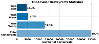
Figure 1: Statistics of restaurants on TripAdvisor.

However, the basic information and user contributed photos of restaurants cannot satisfy all the needs from users. Consider the situation that someone wants to celebrate a wedding anniversary with his wife and has no idea which restaurant is the best. Or he needs to schedule a dinner meeting with his clients and wonders which restaurant is conducive for a business conversation. Such demands from users require higher level information of the restaurant and they are not directly available from the restaurant’s basic information. In this paper, we refer to such higher level information as the style of restaurant. Currently, user-review websites either contain no restaurant styles, such as Foursquare, or rely on users feedbacks, such as TripAdvisor. Therefore, for most of the restaurants online, such information is not available. As shown in Figure 1, among the $34,787$ restaurants we extracted from TripAdvisor, only $14.7\%$ of them have style tags. In this paper, we will refer to styles and tags interchangeably. A even smaller percentage of restaurants has user contributed photos to support the style tags. Only $13.2\%$ of the collected restaurants data contain both photos and style tags.

Although the style tags are not commonly available from the user-review websites, fortunately, it is possible that they can be derived from the user contributed photos , which have a much higher availability. For example, if we see photos from a restaurant containing delicate dishes and romantic decorations, we can infer that this restaurant is suitable for a wedding anniversary or Valentine’s Day dinner. Hence, we propose a restaurant style inference method based on the analysis of the user contributed photos in user-review websites. There are multiple applications for the proposed system: 1) For a given restaurant, it can estimate a collection of highly related restaurant styles from user contributed photos; 2) It can then be used to guide user-review sites to present more useful information of restaurants. The additional availability of the restaurant style tags can help users to search particular types of restaurants; 3) For a restaurant without photos, our method can be used to present a collection of strongly related images that match the style tags of the restaurant. Thus, the users can have a good idea about the style of such a restaurant even without seeing the true images of the exact restaurant; 4) The model can help the restaurants to select the best photos to advertise their restaurant styles; and 5) The trained models can be used by other websites and services related to restaurants.

Inferring restaurant styles from user-uploaded photos can be best described as a multi-instance multi-label learning (MIML) problem [1] where each object (i.e., restaurant) is described by a set of instances (i.e., user-uploaded photos) and associated with several class labels (i.e., restaurant style tags). Traditional MIML problems usually assume that 1) each instance contributes equally and independently to the object’s class label; 2) or there exists a “key” instance that contributes the object’s class label. However, for the restaurant style classification problem such assumptions do not hold. Instead, it is the collection of “key” instances that decide the object’s class label. Based on such assumption, we propose a deep MIML approach to address this problem. We train a multi-label CNN for two rounds in a bootstrap fashion. We then use the trained multi-label CNN in combining with a restaurant profiling algorithm to extract restaurant style features from the collection of images of a restaurant. Next, we feed the extracted features to a set of SVMs to obtain the restaurant style tags. Our experimental results show that the proposed method is indeed effective in predicting the style tags of a restaurant and a F-1 score of 0.58 is achieved.

The remainder of this paper is organized as follows. In Section II, we present on the related work. In Section III, we introduce the procedure of data collection and statistics of the collected dataset. The proposed framework and detailed algorithms used in our method are described in Section IV. We evaluate the performance of our method in Section V and conclusions are given in Section VI.

II Related Work

II-A Related Work in Social Media

Mining data from user-review websites is popular in recent years [2, 3, 4, Wang:2010:LAR:1835804.1835903, 5, 6]. However, only a few of them focus on data mining on restaurants [7, 8, 9, 10, 11]. Aside from our work, which uses visual information, most these restaurant related works only use restaurant meta data, user reviews, or geographic information to provide restaurant recommendations to users [9, 8, 11] and none of them is able to provide higher level recommendations, such as restaurant styles. Other venue related works make use of visual information to decide which venues should be recommended [6, 12, 13, 14]. In particular, [6] uses deep neural networks to extract useful features in images. What sets our work apart from this work is that we focus more on the restaurant styles, which is highly abstract, while they mainly concentrate on general and more concrete aspects of a venue.

II-B Related Work on Multiple Instance Multiple Label Learning

The formal definition of a MIML framework is given by Zhou et al [1]. They proposed two ways of targeting the MIML problem: 1) Degenerating the MIML problem to a multi-instance learning problem and solving the problem with a multi-instance learner; 2) Degenerating the MIML problem to a multi-label learning problem and solving the problem with a multi-label learner. However, existing MIML algorithms [15, 16, 17] are not applicable to our restaurant style classification problem. [16] assumes that all the instances contribute equally to the object’s labels. However, in our case, there are a number of uninformative images, such as pictures of common dishes and images of the dinning tables. They contribute very little to the restaurant’s style. [15, 16] are only feasible when the numbers of possible instances and objects are not large. While, in our case, we need to train and test our model on a large-scale dataset (See Table I). [17] is provably efficient to work on large datasets. However, it assumes that the object is positive if and only if there exists at least one positive instance. In our case, such assumption is not guaranteed. For example, just one picture of a delicate dish does not mean the restaurant itself is romantic.

II-C Related Work on Convolutional Neural Network

In recent years, deep convolutional neural networks (CNNs) have shown to be very successful in lots of machine learning tasks. In relating to our problem, some literatures target the multi-instance learning problems using CNNs. Pathak et al. [18] proposed a novel multi-instance learning algorithm for semantic segmentation using CNNs. The proposed algorithm try to learn pixel-level semantic segmentation only based on the weak image-level labels, while in our case we need to learn image-level labels from bag-level restaurant labels. Wu et al. [19] showed that deep learning based multi-instance learning can be very useful in image classification and auto-image notation. The authors try to classify images based on a set of generated image proposals and therefore the proposed algorithm relies heavily on the assumption that if there exists at least one positive proposal then the image itself is positive. However, such assumption does not hold for our restaurant classification problem. There are some other works focus on solving multi-label learning problems using CNNs. Wei et al. [20] proposed a deep CNN infrastructure, called Hypotheses-CNN-Pooling, for multi-label image classification. Gong et al. [21] investigated the choices of different loss functions on the performance of multi-label image annotation using CNNs. However, none of these works consider the MIML problem using CNNs, which sets our work apart from existing CNNs algorithms.

III Data collection

Cities	# of Restaurants	# of Photos
Chicago	7150	32676
Houston	6732	14084
Los Angeles	7903	22379
New York City	9871	128657
Miami	3131	19672
Total	34787	217468

TABLE I: Restaurant statistics of five major US cities.

Restaurant Styles From TripAdvisor
Bar scene	Local cuisine
Business meeting	Romantic
Dining on a budget	Scenic view
Families with children	Special occasions
Large groups

TABLE II: Restaurant styles in TripAdvisor.

All of our data are collected from TripAdvisor. We choose TripAdvisor because some of its restaurants contain user labeled style tags. We can use them as the pseudo ground truth to guide the training of a multi-label CNN, which will be discussed in Section IV-A. However, as we have mentioned in Section I, for most of the restaurants, the style tags are not available. Therefore, we still need to use the trained framework in Section IV to assign them restaurant styles based on the associated user contributed photos.

To make sure the restaurant photos we use are representative, we choose restaurants from five major cities in the United States. A list of cities with the number of restaurants and photos is given in Table I. In total, our data set contains $34,787$ restaurants and $217,468$ photos. According to TripAdvisor’s taxonomy, there are in general 9 restaurant styles. The taxonomy of these styles is shown in Table II.

IV Methodology

The framework of our approach is illustrated in Figure 2. The flowchart at the top demonstrates the training phase and the bottom represents the testing phase. For a given restaurant, our goal is to detect a collection of applicable restaurant styles from user contributed photos. To deal with this MIML learning task, we adapt the idea from [1]: reducing the task to a multi-label learning task and solving it with a multi-label learner. In a high level view, our proposed framework extracts the features of a restaurant from a bag of images using CNNs and then feeds the features to a series of binary SVMs to obtain the restaurant styles.

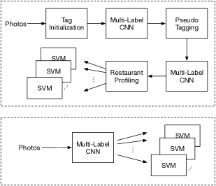
Figure 2: Illustration of the framework of our method. Top: training phase. Bottom: testing phase.

In the training phase, we build a multi-label CNN that can infer the style features represented by the collection of user-contributed photos from a restaurant. For each photo, the multi-label CNN outputs a vector of scores where each score indicates the confidence of the photo relating to a restaurant style. The score vectors will be used to obtain the style features of a restaurant. However, due to the multi-instance learning nature of our problem, the challenge we face is that we do not have individually labeled photos for direct training. The only information we have is the style tags of the restaurants, which are supplied by users (and can be noisy). To solve this problem, we propose to train the multi-label CNN for two rounds in a bootstrap fashion. As illustrated in Figure 2, the first round CNN plus the pseudo tagging algorithm is used to estimate the labels of each image in the restaurant. Then, we train the second round CNN based on the labeled images and use this CNN to extract restaurant style features in the test phase. Notice that there is no need to train for the third round (or even further). As we will then train and test on the same dataset and there will not be any performance gain using the pseudo tagging algorithm.

In the first round, we aggressively initialize the tags of each photo according to its restaurant style tags, i.e., all the images from the same restaurant will have the same style tags as the restaurant. Note that such assignment of tags may result lots of false positives and negatives. Based on our observations, most of the false positives and negatives relate to uninformative images. They frequently appear across restaurants and contain no information that indicate specific styles. Those uninformative images are not considered as noise for the multi-label CNN, as their contribution to each restaurant styles will be canceled out during the optimization process of the training. In the cases that false positives and negatives are actually informative images, the multi-label CNN training may be degraded by those images. However, such cases are not frequent, otherwise the tags of the corresponding restaurants would be changed. Therefore, in general the assignments of photos with their restaurant’s tags are reasonable and the trained multi-label CNN classifier should give us good estimates of labels of individual images. The output of our multi-label CNN is a $9$-dimension score vector, where each score represents the weight of the image on the corresponding tag. We will discuss more details of the structure of the multi-label CNN model in Section IV-A and a set of top scored photos is shown in Figure 4.

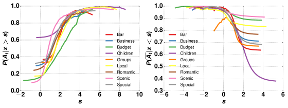
Figure 3: The probability relation between photo scores and restaurant styles. Given a photo with a score $x$ on tag $t$ greater than $s$, the probability of its restaurant has a style $t$ is denoted by $P(A_{t}|x>s)$. Given a photo with a score $x$ on tag $t$ less than $s$, the probability of its restaurant has no style $t$ is denoted by $P(\overline{A_{t}}|x<s)$. Here, the scores of photos are computed from the first round multi-label CNN. $P(A_{t}|x>s)$ and $P(\overline{A_{t}}|x<s)$ for each tag are calculated using Equations (4) and (5).

Before training the multi-label CNN for the second round, we use a pseudo tagging algorithm to relabel the tags of each image in the training set. Basically, this algorithm takes the scores of each image as an indicator of being relevant to the tags and remove the presumably false negatives and positives accordingly. The details of this algorithm are given in section IV-B. There are two reasons that we need this algorithm and the second round multi-label CNN. First, the pseudo tagging algorithm can remove some incorrectly labeled informative images and thus can improve the performance of the second round multi-label CNN. Second, the pseudo tagging algorithm rewards higher scored images and punishes lower scored images by adding and removing the corresponding tags. Thus, the outputs of the second round multi-label CNN will be more sensitive to those images that have higher similarity with the top scored images in the training set. Such a sensitivity would be helpful to extract better restaurant features in the restaurant profiling phase. Based on the scores of images, we extract the features of each restaurant using the restaurant profiling algorithm, which we shall discuss more details in Section IV-C. We then train $9$ binary classifiers using SVM, and the outputs of the classifiers give the tags of the restaurants.

Finally, in the testing phase, we use the entire collection of photos from a restaurant as the input. Next, compute their scores using the second round multi-label CNN model. For each label, we extract the restaurant’s features using the top-$k$ scores and use the output of the SVM classifiers to derive the restaurant styles.

IV-A Multi-label CNN

IV-A1 Test

As we have discussed in the previous section, our approach uses the multi-label CNN to evaluate each image of a restaurant. The multi-label CNN outputs the score vectors that will be further used to obtain the style features of a restaurant. Here, each score indicates the confidence of the photo being related to a restaurant style.

Formally put, let $\mathbf{X}_{i}$ and $\mathbf{Y}_{i}$ denote the images and the associated tags, respectively. The associated tags $\mathbf{Y}_{i}=[y_{i}^{1},y_{i}^{2},\dots,y_{i}^{L}]^{T}$ is a binary vector, where

$$y_{i}^{t}=\begin{cases}1,\text{if tag }t\text{ belongs to }\mathbf{X}_{i},\\ 0,\text{otherwise.}\end{cases}$$ (1)

and $L$ is the total number of tags (in this work $L=9$). Due to its high capacity and flexibility, CNN has become a common framework to learn image representation that adapts to specific domains [22]. CNN maps images $\mathbf{X}_{i}$ to a feature space with multiple layers of convolution, pooling, non linear activations and fully connected layers. The final layer of the architecture is designed to output the label confidence scores with respect to the image. Let $\mathbf{S}_{i}=[s_{i}^{1},s_{i}^{2},\dots,s_{i}^{L}]^{T}$ denotes the score vector with respect to $\mathbf{X}_{i}$. A proper loss function $l(\mathbf{S}_{i},\mathbf{Y}_{i})$ is designed over the score vector $\mathbf{S}_{i}$ to learn the weights $\theta$ in the CNN architecture using stochastic gradient descent (SGD),

$$\theta:=\theta-\alpha\sum_{i}\nabla_{\theta}l(\mathbf{S}_{i},\mathbf{Y}_{i};\theta),$$ (2)

where $\theta$ denotes the network parameters to be learned from the training dataset and $\alpha$ is the learning rate for the optimization algorithm. We use the cross entropy sigmoid loss function [23, Chapter 3] as our form of $l(\mathbf{S}_{i},\mathbf{Y}_{i})$,

$$l(\mathbf{S}_{i},\mathbf{Y}_{i})\triangleq\sum_{t}y_{i}^{t}\sigma(s_{i}^{t})+(1-y_{i}^{t})(1-\sigma(s_{i}^{t})),$$ (3)

where $\sigma$ is the sigmoid function $\sigma(x)=1/(1+\exp(-x))$ which transforms label confidence into probabilities. The objective of (3) is to maximize the confidence of the labels in the target $\mathbf{Y}_{i}$ and suppress those not in the target $\mathbf{Y}_{i}$. From (3), we compute the gradients of the loss function with respect to the label confidence $\mathbf{S}_{i}$, which is used to compute $\nabla_{\theta}l(\mathbf{S}_{i},\mathbf{Y}_{i};\theta)$ for the stochastic gradient descent algorithm by applying chain rules. This process is also called backpropagation.

IV-B Pseudo Tagging

As mentioned in Section IV, we do not have the ground truth of the individual training images. Therefore, we use the first round multi-label CNN combined with the pseudo tagging algorithm to estimate the labels of the training images. The pseudo tagging algorithm is based on the following assumption:

• Images with the highest scores are likely to be related to the tag and images with the lowest scores are likely to be unrelated to the tag.

This assumption is based on the analysis and observation that the first round multi-label CNN training in general provides a good indication of being relevant to the tags. It can be further verified using the following conditional probabilities. Let $A_{t}$ be the event that a given style tag $t$ should be assigned to the restaurant $A$ and $x$ be the confidence score of an image. Thus, given that an image has the score $x$ greater than $s$, the probability of event $A_{t}$ can be estimated by

$$P(A_{t}|x>s)=\frac{C(A_{t},x>s)}{C(x>s)}.$$ (4)

Here, $C(A_{t},x>s)$ is the number of images whose restaurant tag is $t$ and have a score on $t$ greater than $s$. $C(x>s)$ is the total number of images whose score on $t$ is greater than $s$. Note that we do not aggregate images from the same restaurant yet as we only focus on the score effectiveness of individual images. As long as we have the scores of training images from the first round multi-label CNN. $C(A_{t},x>s)$ and $C(x>s)$ can be easily counted. Similarly, we can estimate $P(\overline{A_{t}}|x<s)$ by

$$P(\overline{A_{t}}|x<s)=\frac{C(\overline{A_{t}},x<s)}{C(x<s)}.$$ (5)

where $\overline{A_{t}}$ denotes the event that tag $t$ is not assigned to restaurant $A$. The probability distribution of $P(A_{t}|x>s)$ and $P(\overline{A_{t}}|x<s)$ among the training photos is shown in Figure 3. In the left figure, we can see that in general when the score of a photo is high on a tag, then it is very possible that its restaurant will also be assigned to this tag. Similarly, in the right figure, those lower scored images on tag $t$ are more likely coming from restaurants without style $t$. Detailed discussion of this experimental result is given in Section V-A.

Let $\mathbf{X}_{m,n}$ be the $m$th image of the $n$th restaurant in the training set, $\mathbf{S}_{m,n}=[s_{m,n}^{1},s_{m,n}^{2},\dots,s_{m,n}^{L}]^{T}$ be the score vector with respect to $\mathbf{X}_{m,n}$, and $\mathbf{Y}_{m,n}=[y_{m,n}^{1},y_{m,n}^{2},\dots,y_{m,n}^{L}]^{T}$ be the binary label vector associated with $\mathbf{X}_{m,n}$, where

$$y_{m,n}^{t}=\begin{cases}1,\text{ if tag }t\text{ belongs to }\mathbf{X}_{m,n},\\ 0,\text{ otherwise.}\end{cases}$$ (6)

and $L$ is the total number of possible tags in the dataset. The score vector $\mathbf{S}_{m,n}$ can be obtained from the multi-label CNN which we trained in the first round. Since $s_{m,n}^{t}$ denotes the confidence of assigning tag $t$ to $\mathbf{X}_{m,n}$ and a higher score denotes a higher confidence, we can estimate the binary label vector $\mathbf{Y}_{m,n}$ using $\mathbf{S}_{m,n}$. To this end, we propose the following algorithm:

1.

Initialize all the images in the training set with their restaurant tags, i.e., $\forall m,n$, $\mathbf{Y}_{m,n}=\mathbf{Y}_{n}$, where $\mathbf{Y}_{n}$ denotes the binary label vector of the $n$th restaurant.

2.

For each image $\mathbf{X}_{m,n}$ in the training set, compute their score vector $\mathbf{S}_{m,n}$ using the multi-label CNN.

For

each tag $t$ do

3.

Pick the image $\mathbf{X}_{a,b}$ that has the highest score $s_{a,b}^{t}$ among all the images that do not have tag $t$ and assign $t$ to $\mathbf{X}_{a,b}$, i.e., pick

$$a,b=\operatorname*{arg\,max}_{m,n}\{s_{m,n}^{t}\mid y_{m,n}^{t}=0\}$$ (7)

and set $y_{a,b}^{t}=1$.

4.

Pick the image $\mathbf{X}_{c,d}$ that has the lowest score $s_{c,d}^{t}$ among all the images that have tag $t$ and remove $t$ from $\mathbf{X}_{c,d}$, i.e., pick

$$c,d=\operatorname*{arg\,min}_{m,n}\{s_{m,n}^{t}\mid y_{m,n}^{t}=1\}$$ (8)

and set $y_{c,d}^{t}=0$.

5

If $s_{a,b}^{t}-s_{c,d}^{t}>const$, go to step $3$.

End for

Here, in step $3$ and $4$, each time we only alter the tag of the image that has the highest possibility that it was incorrectly labeled. For example, in step $3$, the algorithm searches the image that does not have tag $t$ but has a relatively high confidence score on $t$ (the highest among all the images that are not labeled with $t$). As such an image is very likely to be incorrectly labeled, we flip its label (from $0$ to $1$). Therefore, in general, this algorithm will yield a better estimation of the tags in each iteration.

In each iteration of the inner-loop, the confidence scores on tag $t$ of image $\mathbf{X}_{a,b}$ and $\mathbf{X}_{c,d}$ will keep on decreasing and increasing, respectively. This is because we always flip the tags of images with highest (in step $3$) or lowest (in step $4$) confidence scores. When the difference of $s_{a,b}^{t}$ and $s_{c,d}^{t}$ becomes very small, the multi-label CNN has a low confidence in classifying $\mathbf{X}_{a,b}$ and $\mathbf{X}_{c,d}$ correctly. In this case, image $\mathbf{X}_{a,b}$ and $\mathbf{X}_{c,d}$ are actually uninformative images. Since the flipping of tags of $\mathbf{X}_{a,b}$ and $\mathbf{X}_{c,d}$ will not help us distinguish the informative images, we should then stop the label estimation with respect to tag $t$ and move on to the next tag. Note that as we only want to find the informative images of each restaurant, those incorrectly labeled uninformative images will not degrade the performance of the multi-label CNN and that is why we call this algorithm pseudo tagging. The parameter $const$ in the stop condition of step $5$ is chosen empirically based on the score distribution of the uninformative images. The pseudo tagged photos are used to train the multi-label CNN for the second round. The image scores computed by the second round CNN will then be used for restaurant profiling.

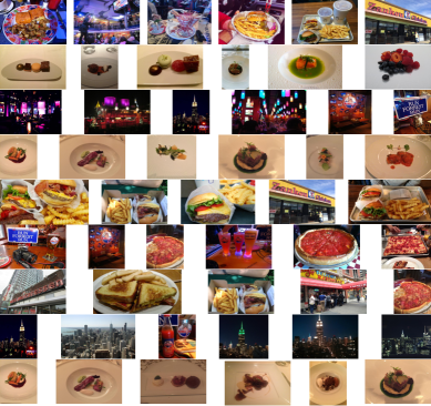
Figure 4: Top scored photos. From top to bottom rows: Family with children, romantic, bar scene, business meetings, dining on a budget, large groups, local cuisine, scenic view, special occasions.

IV-C Restaurant Profiling

To infer the styles of a restaurant, we need to extract the restaurant features from a collection of photos. However, for a restaurant with a given style, not all the photos are necessarily related to this style. In fact, in most of the cases, only a small portion of the images will be useful. For example, for a “bar scene” style, we are usually looking for glasses or bottles of wine, bar counters, and dark scenes with a group of people drinking alcohol. Therefore, images of regular dishes or foods will not contribute much to our decision. However, usually most of the user contributed photos are related to the dishes themselves instead of the “bar scene”. To this end, we design a restaurant profiling algorithm, which is based on the following assumption:

• The tag of a restaurant is determined by a number of informative images. If a restaurant is labeled with a certain tag, there must be a number of images that are highly related to this tag.

Based on this assumption, we use the photo scores computed by the multi-label CNN as an indicator of informativeness. As a higher score means a higher possibility an image is relevant to a tag, top scored images always have a better chance that they are the informative images. Thus, we pick the top-$k$ scored images as the candidates of the informative images and choose their scores as the extracted features on a given tag. Here, $k$ denotes the number of the photos we choose to treat as the informative images of a restaurant. We will discuss more about the choice of $k$ in Section V-C.

Formally put, let $\mathbf{G}_{n}^{t}=[s_{1,n}^{t},s_{2,n}^{t},\dots,s_{M_{n},n}^{t}]^{T}$ be the score vector of the $n$th restaurant with respect to tag $t$, where $s_{m,n}^{t}$, $m\in\{1,\dots,M_{n}\}$, denotes the confidence score of image $\mathbf{X}_{m,n}$ with respect to tag $t$. $M_{n}$ is the total the number of images in the $n$th restaurant. Thus, following the discussion above, we can use the $k$-largest elements of $\mathbf{G}_{n}^{t}$ as the feature vector of the $n$th restaurant on tag $t$. We denote such feature vector as $\mathbf{F}_{n}^{t}$. Then, for each tag $t$, we can train a binary classifier $C^{t}$ using any linear discriminative model, such as SVM. The procedure of the algorithm is given in Algorithm 1. Here, $L$ is the total number of the tags and $N$ is the total number of restaurants in the training set.

Algorithm 1 Restaurant profiling algorithm

1:procedure Restaurant Profiling($k$)

2:     for $n\in\{1,2,\dots,N\}$ do

3:         for $m\in\{1,2,\dots,M_{n}\}$ do

4:              $\mathbf{S}_{m,n}\leftarrow$ compute the score vector of image $\mathbf{X}_{m,n}$

5:         end for

6:     end for

7:     for $t\in\{1,2,\dots,L\}$ do

8:         for $n\in\{1,2,\dots,N\}$ do

9:              $\mathbf{G}_{n}^{t}\leftarrow[s_{1,n}^{t},s_{2,n}^{t},\dots,s_{M_{n},n}^{t}]^{T}$

10:              $\mathbf{F}_{n}^{t}\leftarrow$ $k$-largest elements of $\mathbf{G}_{n}^{t}$

11:         end for

12:         $\mathbf{F}^{t}\leftarrow\{\mathbf{F}_{1}^{t},\mathbf{F}_{2}^{t},\dots,\mathbf{F}_{N}^{t}\}$

13:         $C^{t}\leftarrow$ train a binary classifier using $\mathbf{F}^{t}$

14:     end for

15:     $\mathbf{C}\leftarrow\{C^{1},C^{2},\dots,C^{L}\}$

16:     return $\mathbf{C}$

17:end procedure

V Experimental Results

In our experiments, we choose the restaurants that contains both user contributed photos and user labeled tags for training and testing. Among the $34,787$ restaurants we tracked, $4,573$ satisfy this requirement. We use 5-fold cross-validation for training and testing. In the training phase, $113,550$ photos are used to train the multi-label CNN models. We use the BVLC Caffe deep learning framework [24] to perform all the CNN training and testing. For hyper parameters, we follow the standard practice on ImageNet challenges[25], i.e., batch size $=256$, learning rate $=0.001$, momentum $=0.9$ and weight decay $=5e-06$. The network is fine tuned from the Alexnet [22], which was the early winning entry of the ImageNet challenges and considered adequate for this study (although other network structures may provide marginal improvements). The optimization converges after $5$ epochs. GPUs are used to accelerate our experiments.

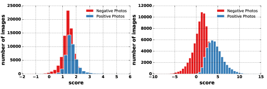
(a) Bar scene

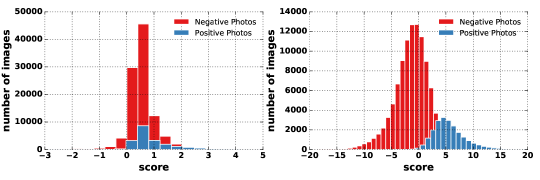
(b) Local cuisine

Figure 5: Distributions of image scores on the “bar scene” and “local cuisine” tags. First column: image scores computed from the first round multi-label CNN. Second column: image scores computed from the second round multi-label CNN. Negative photos are those photos without the “bar scene”/“local cuisine” tag. Positive photos are those photos tagged with “bar scene”/“local cuisine” tags.

V-A Performance of Multi-label CNN

For an input image, the multi-label CNN model will output a vector of scores where each element as the score of the corresponding tag. Ideally, for an image that is strongly related to the style tag $t$, our multi-label CNN should output a relatively high score on $t$. On the other hand, if an image is irrelevant to the tag $t$, then its corresponding score from CNN should be relatively low. Figure 4 shows some top scored images of different restaurant styles. Not surprisingly, photos with a higher score on the “family with children” style mostly contain fast foods or snacks, which are very popular among children. Those photos that receive the top scores on the “romantic” style usually contain delicate dishes or desserts, which are favored by lovers. Finally, for the “bar scene” style, top scored images are often dark with neon lights and contain people drinking wine or beer. Top scored photos in other rows also show strong relations to their corresponding tags. It is also very interesting to observe that the top scored images of “romantic”, “business meetings”, and “special occasions” styles are very similar. It is reasonable as a restaurant, which is good for “special occasions”, is usually also a good place for “romantic” scenes or “business meetings”.

There are also some interesting mistakes. The last image of the second row just contains some fruits. However, our multi-label CNN gives it a relative high score on the “romantic” tag. The reason for this situation is that in most of the cases, a “romantic” photo contains some delicate food that placed in a big white plate. It looks like the multi-label CNN has learned that in general a photo with “romantic” tag should have a white background. Hence, the fruit image gets a high score on the “romantic” tag. Another mistake can be found in the last two images of the “bar scene” row. Apparently, these two images only contain the logos of the restaurants and are not related to the “bar scene”. The reason for this mistake is that these two restaurants are “bar scene” restaurants and lots of photos contain the logos of these two restaurants in our training set. Therefore, the logos are learned by the multi-label CNN to the extent that images containing such logos will get a high score on the “bar scene” tag.

To further evaluate the performance of the multi-label CNN, we use the two conditional probability equations discussed in Section IV-B. The basic idea of using these two equations is if we see an image with a very high score on a certain tag $t$, then it is very possible that the image’s corresponding restaurant has a style $t$. Similarly, if an image get a very low score on tag $t$, then it is unlikely that the corresponding restaurant has a style $t$. For Equation (4), we compute $P(A_{t}|x>s)$ by counting the proportion of the images whose restaurant has a style $t$ among all the images with a score greater than $s$. For different values of $s$, we calculate the conditional probability $P(A_{t}|x>s)$ and the final probability distribution is given in Figure 3. We can see from the left figure that when the score $x$ on a tag $t$ is high, the probability $P(A_{t}|x>s)$ is also very high. This observation is consistent with our assumption. A similar analysis can also be applied to Equation (5). Therefore, we can conclude that the trained multi-label CNN performs well as expected on our dataset.

Styles	Baseline			Proposed Method
	Rec(%)	Prec(%)	F-1 score(%)	Rec(%)	Prec(%)	F-1 score(%)
Bar scene	100.00	36.69	53.68	80.39	48.81	60.74
Business meeting	37.21	84.21	51.61	76.74	52.38	62.26
Dining on a budget	11.76	100.00	21.05	94.12	35.56	51.61
Families with children	100.00	67.15	80.35	77.17	86.59	81.61
Large groups	71.67	39.45	50.89	58.33	50.72	54.26
Local cuisine	3.85	33.33	6.90	69.23	48.65	57.14
Romantic	17.24	100.00	29.41	89.66	35.14	50.49
Scenic view	14.29	100.00	25.00	71.43	17.86	28.57
Special occasions	37.04	80.00	50.63	90.74	68.06	77.78
Average	43.67	71.20	41.06	78.65	49.31	58.27

TABLE III: Performance of the baseline method and the proposed method on different style tags. Here, we choose $k^{\prime}=3$ and the minimum number of photos is $50$. Note that the F-1 scores have improved across all the styles due to the proposed method.

V-B Performance of Pseudo Tagging

As we have discussed in Section V-A, the photo scores output by the first round multi-label CNN are good indicators of the style tags. As shown in Figure 3, the first round multi-label CNN performs very well when the score is very high or very low. However, when the score of an image falls in the middle, it is difficult to tell whether it belongs to the style tag or not.

Figure 5 shows the score distributions before and after using the pseudo tagging algorithm. Here, the first row shows the image score distributions of the “bar scene” tag. The second row shows the image score distributions of the “local cuisine” tag. The figures in the first column show the distributions of image scores computed from the first round multi-label CNN. For the “bar scene” tag, most of the images have a score between $1$ and $2$ while the positive and negative images are mixed together. It means for images with scores between $1$ and $2$, the first round multi-label CNN model cannot distinguish their styles. This is also the case for the “local cuisine” tag. After applying the pseudo tagging algorithm to our training set, we train the multi-label CNN for the second round and the distributions of the computed image scores are shown in the second column of Figure 5. We can find that in this case negative and positive images do not mix as much as before, which means the second round multi-label CNN has a better performance in distinguishing the styles of images. Therefore, the binary classifier training in the restaurant profiling algorithm can benefit significantly from the better separated score distributions. We can also see that our pseudo tagging algorithm helps in separating the score distribution of the “local cuisine” tag. That is why there is a much improved performance gain for the “local cuisine” tag in Table III.

V-C Overall Performance

To show the performance gain from the pseudo tagging and the restaurant profiling algorithm, we also establish a baseline for comparison. For the baseline method, we only train the multi-label CNN once and assign top-$k^{\prime}$ scored tags to photos. If more than a half of the photos are assigned a particular tag, the restaurant is determined to be labeled as such.

In our experiments, we test the performance of the baseline method and our proposed method on a variety of choices of $k^{\prime}$ and $k$. We notice that the more photos a restaurant have, the more information about the restaurant’s styles we can extract. Therefore, we also set different minimum numbers of photos to restaurants in the test set. The performances of the two methods with the best parameter settings are given in Table III. Following the evaluation methods in [26, 16], we use recall, precision, and F-1 measure as the metrics to evaluate the performances of the two methods on different style tags. We can see from Table III that, in general, the proposed method performs much better than the baseline method. It means that the pseudo tagging and the restaurant profiling algorithms play a key role in improving the performance of the proposed method. An interesting finding here is that the “scenic view” style has a very low precision. A closer look at the dataset finds that there are a number of the restaurants contain outdoor images. But those restaurants cannot be considered as typical “scenic view” style restaurant and are not labeled with the “scenic view” tag.

We also investigate the performance differences of our proposed method when choosing different parameter settings. From Figure 6, we can find that the choice of $k$ does not affect the performance much. However, when we choose the restaurants with a higher minimum number of photos the performance gets better. It means when the number of photos of a restaurant is high, our proposed method can achive more accurate estimates of the restaurant styles.

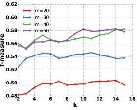
Figure 6: The average f-measure scores of our method when choosing different $k$ and minimum numbers of photos.

VI Conclusions

We have presented a novel approach to profiling restaurant styles directly from user uploaded photos on user-review sites. We propose to build a deep MIML framework to deal with the special problem setting of restaurant style classification. Due to the absence of individual photo tags, we initially train the multi-label CNN using photos labeled with all the restaurant tags supplied by users. We then refine the photo tags using our pseudo tagging algorithm and train the multi-label CNN for a second round. Experiments show that the multi-label CNN performs very well in inferring the restaurant styles, and the pseudo tagging algorithm plays a key role in helping the multi-label CNN to distinguish different restaurant styles. Finally, the photo-level style estimates are used by the restaurant profiling algorithm to train a binary classifier for each style tags using SVM. Our experimental results show that our approach has achieved a significant performance gain due to the pseudo tagging and restaurant profiling algorithms. We also show that when the number of photos of a restaurant increases, the performance of our approach increases as well.

References

- [1] Z. hua Zhou and M. ling Zhang, “Multi-instance multi-label learning with application to scene classification,” in Advances in Neural Information Processing Systems 19, B. Schölkopf, J. C. Platt, and T. Hoffman, Eds. MIT Press, 2007, pp. 1609–1616.
- [2] A. Noulas, S. Scellato, N. Lathia, and C. Mascolo, “Mining user mobility features for next place prediction in location-based services,” in Data Mining (ICDM), 2012 IEEE 12th International Conference on, Dec 2012, pp. 1038–1043.
- [3] Z. Cheng, J. Caverlee, K. Lee, and D. Z. Sui, “Exploring millions of footprints in location sharing services.” ICWSM, vol. 2011, pp. 81–88, 2011.
- [4] Q. Yuan, G. Cong, Z. Ma, A. Sun, and N. M. Thalmann, “Time-aware point-of-interest recommendation,” in Proceedings of the 36th International ACM SIGIR Conference on Research and Development in Information Retrieval, ser. SIGIR ’13. New York, NY, USA: ACM, 2013, pp. 363–372.
- [5] A. Ghose, P. G. Ipeirotis, and B. Li, “Designing ranking systems for hotels on travel search engines by mining user-generated and crowdsourced content,” Marketing Science, vol. 31, no. 3, pp. 493–520, 2012.
- [6] J. Zahálka, S. Rudinac, and M. Worring, “New yorker melange: Interactive brew of personalized venue recommendations,” in Proceedings of the 22Nd ACM International Conference on Multimedia, ser. MM ’14. New York, NY, USA: ACM, 2014, pp. 205–208.
- [7] L. Mui, P. Szolovits, and C. Ang, “Collaborative sanctioning: Applications in restaurant recommendations based on reputation,” in Proceedings of the Fifth International Conference on Autonomous Agents, ser. AGENTS ’01. New York, NY, USA: ACM, 2001, pp. 118–119.
- [8] H.-W. Tung and V.-W. Soo, “A personalized restaurant recommender agent for mobile e-service,” in e-Technology, e-Commerce and e-Service, 2004. EEE ’04. 2004 IEEE International Conference on, March 2004, pp. 259–262.
- [9] B.-H. Lee, H.-N. Kim, J.-G. Jung, and G.-S. Jo, “Location-based service with context data for a restaurant recommendation,” in Database and Expert Systems Applications. Springer, 2006, pp. 430–438.
- [10] L.-M. Liu, S. Bhattacharyya, S. L. Sclove, R. Chen, and W. J. Lattyak, “Data mining on time series: an illustration using fast-food restaurant franchise data,” Computational Statistics & Data Analysis, vol. 37, no. 4, pp. 455 – 476, 2001.
- [11] Y. Fu, B. Liu, Y. Ge, Z. Yao, and H. Xiong, “User preference learning with multiple information fusion for restaurant recommendation.” in SDM. SIAM, 2014, pp. 470–478.
- [12] S. Rudinac, A. Hanjalic, and M. Larson, “Generating visual summaries of geographic areas using community-contributed images,” Multimedia, IEEE Transactions on, vol. 15, no. 4, pp. 921–932, June 2013.
- [13] C. Kofler, L. Caballero, M. Menendez, V. Occhialini, and M. Larson, “Near2me: An authentic and personalized social media-based recommender for travel destinations,” in Proceedings of the 3rd ACM SIGMM International Workshop on Social Media, ser. WSM ’11. New York, NY, USA: ACM, 2011, pp. 47–52.
- [14] A.-J. Cheng, Y.-Y. Chen, Y.-T. Huang, W. H. Hsu, and H.-Y. M. Liao, “Personalized travel recommendation by mining people attributes from community-contributed photos,” in Proceedings of the 19th ACM International Conference on Multimedia, ser. MM ’11. New York, NY, USA: ACM, 2011, pp. 83–92.
- [15] Z.-J. Zha, X.-S. Hua, T. Mei, J. Wang, G.-J. Qi, and Z. Wang, “Joint multi-label multi-instance learning for image classification,” in Computer Vision and Pattern Recognition, 2008. CVPR 2008. IEEE Conference on, June 2008, pp. 1–8.
- [16] Z.-H. Zhou, M.-L. Zhang, S.-J. Huang, and Y.-F. Li, “Multi-instance multi-label learning,” Artificial Intelligence, vol. 176, no. 1, pp. 2291 – 2320, 2012.
- [17] S.-J. Huang and Z.-H. Zhou, “Fast multi-instance multi-label learning,” arXiv preprint arXiv:1310.2049, 2013.
- [18] D. Pathak, E. Shelhamer, J. Long, and T. Darrell, “Fully convolutional multi-class multiple instance learning,” CoRR, vol. abs/1412.7144, 2014.
- [19] J. Wu, Y. Yu, C. Huang, and K. Yu, “Deep multiple instance learning for image classification and auto-annotation,” in 2015 IEEE Conference on Computer Vision and Pattern Recognition (CVPR), June 2015, pp. 3460–3469.
- [20] Y. Wei, W. Xia, J. Huang, B. Ni, J. Dong, Y. Zhao, and S. Yan, “CNN: single-label to multi-label,” CoRR.
- [21] Y. Gong, Y. Jia, T. Leung, A. Toshev, and S. Ioffe, “Deep convolutional ranking for multilabel image annotation,” CoRR, vol. abs/1312.4894, 2013.
- [22] A. Krizhevsky, I. Sutskever, and G. E. Hinton, “Imagenet classification with deep convolutional neural networks,” in Advances in neural information processing systems, 2012, pp. 1097–1105.
- [23] M. A. Nielsen, Neural Networks and Deep Learning. Determination Press, 2015.
- [24] Y. Jia, E. Shelhamer, J. Donahue, S. Karayev, J. Long, R. Girshick, S. Guadarrama, and T. Darrell, “Caffe: Convolutional architecture for fast feature embedding,” arXiv preprint arXiv:1408.5093, 2014.
- [25] O. Russakovsky, J. Deng, H. Su, J. Krause, S. Satheesh, S. Ma, Z. Huang, A. Karpathy, A. Khosla, M. Bernstein, A. C. Berg, and L. Fei-Fei, “ImageNet Large Scale Visual Recognition Challenge,” International Journal of Computer Vision (IJCV), vol. 115, no. 3, pp. 211–252, 2015.
- [26] O. Yakhnenko and V. Honavar, “Multi-instance multi-label learning for image classification with large vocabularies,” in Proceedings of the British Machine Vision Conference. BMVA Press, 2011, pp. 59.1–59.12.