A Holographic Model for Pseudogap in BCS-BEC Crossover (I): Pairing Fluctuations, Double-Trace Deformation and Dynamics of Bulk Bosonic Fluid

Abstract

We build a holographic model for the pairing fluctuation pseudogap phase in fermionic high temperature superconductivity/superfluidity based on the BCS-BEC crossover scenario. The pseudogap originates from incoherent Cooper pairing and has been observed in recent cold atom experiments. The strength of Cooper pairing and hence the BCS-BEC crossover is controlled by an effective 4-Fermi interaction and we argue that the double-trace deformation for charged scalar operator is a close analog in large N field theories. We employ the double-trace deformed Abelian Higgs model of holographic superconductors and propose that the incoherent fluctuations of the charged scalar in the bulk is the holographic dual of the fluctuating Cooper pairs. Using a Madelung transformation and the velocity-potential formalism, we develop a quantum fluid dynamics as an effective theory for these bulk fluctuations. The new fluid dynamics takes care of the boundary conditions required by AdS/CFT and encodes the vacuum polarization effect in curved spacetime. The pseudogap in conductivity can be related to the plasma oscillation of this bulk fluid.

1 Introduction

Since its discovery less than two decades ago, the AdS/CFT correspondence Maldacena:1997re ; Gubser:1998bc ; Witten:1998qj , or holography, has shed new light not only on the fields of gravity and high energy theories, but also on other areas of physics that are highly driven by experiments, such as nuclear physics, condensed matter and cold atoms. One tremendous success it enjoys over the last decade is the building of holographic superconductor/superfluid models starting in Hartnoll:2008vx ; Hartnoll:2008kx ; Horowitz:2008bn ; Herzog:2008he . It bridges the physics of various phases and phase transitions in strongly interacting field theories at finite densities, such as those studied in the context of high temperature superconductivity, to the physics of the dynamics and instabilities of charged black holes in asymptotic AdS spacetime Gubser:2008px . This is part of the fruitful program now called AdS/CMT Hartnoll:2009sz ; Zaanen:2015oix . Since then, great efforts have been devoted to build various holographic models with different types of black hole instabilities and to identify them with possible interesting phases in the dual field theories.

One of the driving forces behind AdS/CMT is to develop effective field theory descriptions for the phenomena of high temperature superconductivity and superfluidity. In the simplest setup, the pure charged AdS black hole geometry is dual to the gapless normal phase at high temperature Lee:2008xf ; Liu:2009dm ; Cubrovic:2009ye ; Faulkner:2009wj , while at low temperature, the black hole develops charged hair and is dual to the gapped superconducting phase Herzog:2009xv ; Horowitz:2010gk ; Cai:2015cya . However, the actual phase diagrams of high $T_{\mathrm{c}}$ materials measured in laboratories are more complicated. For the family of cuprate materials, there exists a so-called “pseudogap” phase Alloul:1988pg ; Batlogg:1994pg ; Loeser:1996pg ; Ding:1996pg that is still mysterious and has defied a consensus among theorists for a long time Keimer:2014review ; Hashimoto:2014review ; Kordyuk:2015review . This is a region in the phase diagram located in between the superconducting phase and normal phase in the underdoped regime, where a gap exists but no coherent superconductivity develops. Recent advances in experimental techniques have shown stronger evidence in favor of the competing order scenario Fradkin:2014review ; Sachdev:2015review : there exists more than one symmetry breaking pattern in this region and the other orders are responsible for the pseudogap and are competing with the superconducting order. This scenario can be easily incorporated into holographic model building. The competing orders can be achieved in holography by adding more matter fields in the bulk. These matters transform under the same symmetry groups as their dual competing orders, and can trigger black hole instabilities toward formation of various types of hair, in similar ways as the superconducting order does. Such a strategy has been successfully implemented in Kiritsis:2015hoa (and see early references therein) and a phase diagram similar to that of cuprate is produced.

The aforementioned story is a familiar one to holographic model builders; however, it is not the whole story of the pseudogap in high temperature superconductivity and superfluidity. In this paper we want to turn our attention to another pseudogap phenomenon that is similar yet distinct from the cuprate one. Recall that fermionic high temperature superfluidity has also been realized and observed in ultra-cold atomic systems since 2004 Regal:2004zza . For the superfluidity transition temperature $T_{\mathrm{c}}$, in terms of the normalized ratio $T_{\mathrm{c}}/T_{\mathrm{F}}$ where $T_{\mathrm{F}}$ is the Fermi temperature of the system, the cold atoms in the unitary regime can reach a ratio of $0.15$ to $0.2$, the highest of any fermionic superfluid! Later, a pseudogap phase was also detected in such systems Gaebler:2010pg ; Feld:2011pg . These cold atom systems are realized in both three and two spatial dimensions, without an underlying optical lattice. Up to the effect of the harmonic trap, these systems can be roughly viewed as translational invariant and isotropic. The dominant symmetry of the order parameter is $s$-wave, not $d$-wave. All these features make the cold atom systems different from cuprate materials. As the competing order scenario for the pseudogap in cuprates relies on the existence of a two-dimensional lattice and $d$-wave symmetry, it lacks foundation in cold atom systems. Thus the explanation for the pseudogap in cold atoms will be very different from the cuprate counterpart. As the paring mechanism is very well understood in fermionic atom systems, the explanation for the pseudogap is more transparent and can be largely attributed to incoherent Cooper pairing with short coherent length and large fluctuations of the superconducting order parameter. However, this poses challenges to holographic model building. As there is no competing order, introducing additional matter fields in the bulk and allowing the black hole to develop different types of hair does not capture the essence of physics in the dual field theory. This fact essentially confines us to the minimal holographic superconductor models, such as the Abelian Higgs model of Hartnoll:2008vx ; Hartnoll:2008kx ; Herzog:2008he . In this paper, we propose that for the Abelian Higgs model, the incoherent fluctuations of the charged scalar field in the bulk is dual to the pseudogap phase. This is the holographic realization of the pairing fluctuation pseudogap in the BCS-BEC crossover scenario Randeria:2013review ; Chen:2014review ; Levin:2012review ; Levin:2005short ; Zwerger:2012book . We will develop an effective fluid dynamic description for these bosonic bulk fluctuations.

In fact, the pairing fluctuation pseudogap in the BCS-BEC crossover is an example of a family of phenomena that could exist in many quantum field theories, where fluctuations play a crucial role. It offers a broad and generic paradigm and can fit into many field theories of different microscopic details. As holography is viewed to be a generic framework for studying strongly interacting quantum field theories, it is already interesting enough to ask the question on a purely theoretical ground how holography can incorporate this paradigm into it, regardless of its applications on experimental phenomenology. This is another motivation of ours to initiate this project.

Another issue involving the holographic study of high temperature superconductivity is the identification of the second axis of the phase diagram. Unlike conventional fermionic superconductivity and superfluidity, whose phase diagrams are usually one-dimensional and labeled by the normalized temperature $T/T_{\mathrm{F}}$ (whereas in holography $T_{\mathrm{F}}$ is usually replaced by the chemical potential or appropriate power of the charge density), high temperature superconductivity has two-dimensional phase diagrams. The second axis is an external tunable knob in the experiments: doping for cuprates and scattering length for cold atoms. There is no consensus in holography how these shall be realized in the bulk theory. In this paper, we propose to use a double-trace deformation Witten:2001ua as a universal knob for modeling these tunable parameters in holography. This is not a completely new idea, as it has already been employed in the early days of holographic superconductors Faulkner:2010gj ; but an explicit identification with the second axis in high $T_{\mathrm{c}}$ phase diagram was rarely made in the literature. The justification comes from the fact that, although doping and scattering length are quite different at the microscopic level, at low energy due to the renormalization group (RG) flow, they generate the same IR effect: they induce an effective 4-Fermi type interaction between the elementary fermions, and the tunable parameters enter as the dimensionful 4-Fermi coupling. The simplest non-Abelian generalization of such 4-Fermi interaction is the double-trace deformation, where the single-trace operator is made of fermion bilinears and their supersymmetric partners. To make the argument stronger, in this paper, we will show that using the variational principle and the trick of the Hubbard-Stratonovich transformation, the 4-Fermi interaction in condensed matter field theories and the double-trace deformation in high energy field theories have similar structures in the generating functionals, which are mainly characterized by pairing symmetry and a dimensionful coupling parameter. Such structures pass naturally into holography. Now there are two distinct coupling strengths in our field theory: the ’t Hooft coupling of the undeformed theory and the double-trace coupling. As we are working with AdS/CFT, we are always in the large ’t Hooft coupling limit, by which we claim our field theory is always in the strong coupling regime. Meanwhile we can always tune the double-trace coupling from week to strong, which mimics the effect of “doping” the large $N$ field theory. This is thus a large $N$ setup analogous to the theory of the BCS-BEC crossover, from which a pairing fluctuation pseudogap phase will emerge.

This paper is organized as follows. In the next section, we will give an introduction to the experimental observations of the pseudogap in cold atom systems and the pairing fluctuation theory in the BCS-BEC crossover scenario, and discuss what they imply for holographic model building. In Section 3, we set up the Abelian Higgs model of holographic superconductivity with a double-trace deformation, review the basics in a slightly different perspective and discuss how this model will be extended without adding a new bulk field to generate the pairing pseudogap phase. Sections 4 and 5 consist of two steps that transform the conceptual ideas developed in Section 3 into a practically calculable model based on fluid dynamics. Section 6 focuses on the bulk dynamics of the hydrostatic configuration which we propose corresponds to the ground state of the pseudogap. Section 7 discusses bulk dynamics of charges and how the pseudogap in AC conductivity can be related to the oscillations of these charges. Section 8 consists of a summary and comments.

Notation: $d$ is the spacetime dimension of the field theory, hence the bulk has $d+1$ dimensions. $M,N$ denote the bulk spacetime indices. $\mu,\nu$ denote the boundary spacetime indices. $I,J$ denote bulk spatial indices while $i,j$ boundary spatial indices. We also use the notation $\vec{v}$ to denote the boundary spatial vector with components $v^{i}$. We choose the general ansatz for the metric to be

$$ds^{2}=g_{tt}(z)dt^{2}+g_{zz}(z)dz^{2}+g_{\perp}(z)d\vec{x}^{2},$$ (1)

and near the boundary, the asymptotic AdS metric takes the form

$$ds_{\mathrm{AdS}}^{2}=\frac{R^{2}}{z^{2}}\left(-dt^{2}+dz^{2}+d\vec{x}^{2}\right),$$ (2)

where $z\in\left[\epsilon,z_{\mathrm{h}}\right]$ is the radial coordinate, $R$ the AdS radius, $\epsilon\rightarrow 0$ the location of the boundary and $z_{\mathrm{h}}$ the location of the horizon. The stress tensor and charge current operators are defined as

$$T^{MN}=\frac{2}{\sqrt{-g}}\frac{\delta S}{\delta g_{MN}},\qquad J^{M}=\frac{1}{\sqrt{-g}}\frac{\delta S}{\delta A_{M}}.$$

2 BCS-BEC Crossover and Incoherent Cooper Pairing

In this section we give a pedagogical introduction to the experimental facts and theoretical ideas of the BCS-BEC crossover scenario, focusing on physics closely related to the pairing fluctuation pseudogap. For readers interested in more details, we recommend the reviews Randeria:2013review ; Chen:2014review ; Levin:2012review ; Levin:2005short , the book Zwerger:2012book and references therein.

2.1 Experimental Evidences for Pairing Fluctuation Pseudogap

In experiments, a pseudogap is defined as a gradual depletion of the density of state of the elementary fermions near the Fermi surface at a temperature above $T_{\mathrm{c}}$, the onset temperature of superconductivity or superfluidity. It can be directly measured by scattering of the elementary fermions out of the system using techniques such as angle-resolved photoemission spectroscopy (ARPES) in condensed matter Damascelli:2003review ; Damascelli:2002review ; Campuzano:2002review and momentum resolved radio frequency (RF) spectroscopy in cold atoms Stewart:2008rf . In Gaebler:2010pg , a gas of fermionic ${}^{40}\mathrm{K}$ atoms is cooled to a fraction of its Fermi temperature in a three-dimensional trap and tuned close to the unitary regime where the interactions between the atoms are near the strongest. Then using the technique of RF spectroscopy, the single-particle spectral function of the fermionic atoms is measured both below and above $T_{\mathrm{c}}$, and the dispersion relation is retrieved from these measurements. The results are shown in Figure 1, which is directly reproduced from Gaebler:2010pg . The first plot is measured below $T_{\mathrm{c}}$, and the rest above $T_{\mathrm{c}}$. The white dots are fits of the dispersion relation. The black curves are the standard quadratic dispersion relation for non-relativistic free particles, while the white curve is a fit to BCS-type dispersion relation with a non-vanishing energy gap. From the two central plots, it is obvious that the dispersion relation follows the BCS trend very well into temperatures well above $T_{\mathrm{c}}$, indicating the existence of a pseudogap phase above $T_{\mathrm{c}}$.

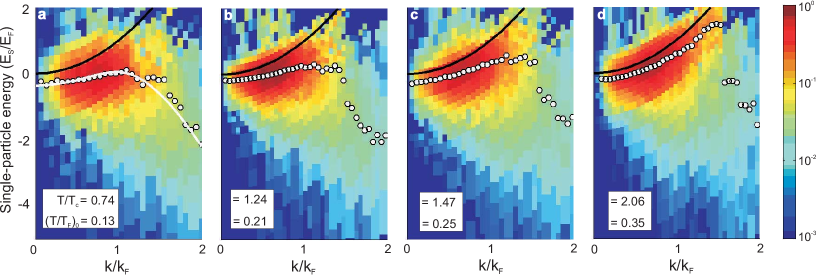
Figure 1: Photoemission spectra throughout the pseudogap regime. Spectra are shown for Fermi gases of ${}^{40}\mathrm{K}$ near unitarity at four different temperatures: the first one below $T_{\mathrm{c}}$, the onset temperature of superfluidity, while the rest above $T_{\mathrm{c}}$. White dots indicate Gaussian fits of the dispersion relation. The black curve is the standard quadratic dispersion relation for non-relativistic free particles. The white curve is a fit to a BCS-like dispersion, indicating the existence of a gap. It is manifest through the two central plots that the gap persists into temperatures well above $T_{\mathrm{c}}$. The figure is reproduced from Gaebler:2010pg .

Later, the same phenomenon was also observed in two-dimensional Fermi gases Feld:2011pg .

Unlike in the cuprate case where the underlying lattice structure, the $d$-wave symmetry and the still mysterious mechanism for Cooper pairing can give rise to many possibilities for competing orders, the cold atom systems are much cleaner and simpler. The interactions between elementary fermions are well understood and the strengths are highly tunable in experiments. The $s$-wave symmetry and the absence of the lattice make it much easier to attribute the observed pseudogap to the incoherent fluctuations of Cooper pairs. This phenomenon has been predicted, long before the experiment of Gaebler:2010pg , by the BCS-BEC crossover scenario, which is originally proposed to explain the pseudogap phenomenon in cuprate materials (for reviews on this topic, see Chen:2000thesis ; Levin:2005long ; Levin:2010review ; Strinati:2010review ). In the following, we will give a brief introduction to the theory of BCS-BEC crossover and how it deals with the pseudogap.

2.2 The BCS-BEC Crossover Scenario

Conventional superconductivity and superfluidity in systems of fermions and bosons are described by the Bardeen–Cooper–Schrieffer (BCS) theory BCS:1957 and the Bose-Einstein Condensation (BEC) theory respectively. The BCS-BEC crossover scenario views these two distinct paradigms as two opposite limits of a unified paradigm that continuously interpolates between them. The central concept of the BCS paradigm of fermionic superconductivity is the Cooper pairing of fermions via attractive interactions. However, the pairing mechanism in the original BCS theory is really a special case that is far from the most general thing that can happen to a pair of fermions. The attractive interaction is so weak that the fermions are only loosely bound. This results in large pair size characterized by a divergent coherence length in position space. In momentum space, the pairing happens near the Fermi surface between momenta of opposite direction. Thus the center of mass momentum of the Cooper pair, i.e. the momentum of this composite boson, is always zero. From the BEC point of view, this is a boson at its ground state, i.e. a condensate. In BCS superconductivity, this boson can only be excited by breaking into two fermions (the Bogoliubov quasi-particles) rather than jumping into an excited bosonic state with non-vanishing momentum, because the attractive interaction between the constituent fermions is so weak that any effort to shake the boson a little bit simply breaks it. The key constituents in the BCS paradigm are the unpaired fermions and paired bosons in the ground state. On the other hand, in the BEC paradigm, we start with a system of bosons. However, a second thought immediately tells us that this is not always true. For example, ${}^{4}\mathrm{He}$ is made of six fermions of electrons, protons and neutrons at the subatomic level and the latter two can be further decomposed into more elementary fermions. Thus the fact that we can start with well defined bosons in the BEC paradigm is really a low energy effective picture, because the attractive interactions that bind the elementary fermions are so strong that the binding energy is way higher than the energy scale at which we probe the system to study superfluidity. This strong interaction results in tightly bound pairs in position space with small coherence length of order of the boson size. In momentum space, the boson, i.e. pair of fermions, can be excited to states with very large momenta without being broken into fermions. We can say the key constituents in the BEC paradigm are the paired bosons in the ground state and excited states, without unpaired fermions. Every feature discussed here in the two paradigms is opposite to the other. However, they are both rooted in the same ground: pairing of two fermions into a boson, and the differences are only quantitative, not qualitative.

We can summarize the BCS-BEC crossover scenario in the following. It describes a system of elementary fermions with tunable attractive interaction. The fermions pair into bosons. The energy scale associated with pairing is the binding energy, which corresponds to an onset temperature $T^{*}$. Below this temperature, the pairs start to form and the binding energy manifests itself as an energy gap in the system which can be directly detected in experiments by scattering the fermions off the system. Once the paired bosons are formed, they can occupy both the ground state and excited states, labeled by different momenta. As the temperature keeps lowering, the paired bosons tend to populate more lower energy states. Eventually at some critical temperature $T_{\mathrm{c}}$, the Bose-Einstein condensation of the boson pairs takes place and the ground state is macroscopically occupied: a coherence starts to form. The pairing temperature $T^{*}$ shall never be lower than the condensation temperature $T_{\mathrm{c}}$: this is simply the statement that the bosons have to form first before they condense. One limiting case is $T^{*}=T_{\mathrm{c}}$, i.e. the pairs condense as soon as they form — this is the BCS limit. The other limiting case is $T^{*}\gg T_{\mathrm{c}}$, where the pairs have already formed even at room temperature which make it looks like we start with bosons — this is the BEC limit. In between these two limit, there is a large regime where the two temperatures are comparable but not equal. This is the regime of unconventional superconductivity and superfluidity for which the BCS-BEC crossover scenario is proposed. Figure 2 is a qualitative phase diagram based on theoretical studies.

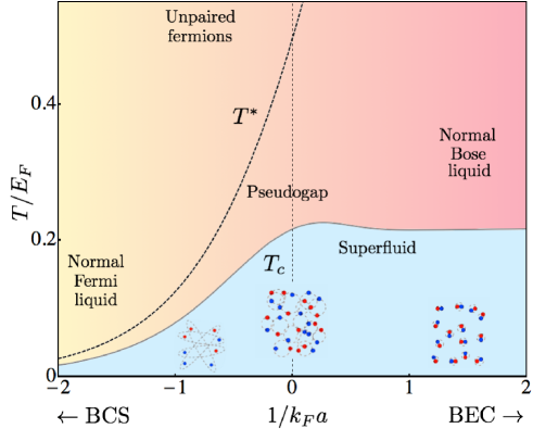
Figure 2: A qualitative illustration of the phase diagram of the BCS-BEC crossover scenario based on theoretical studies. The horizontal axis is the strength of the coupling, in this note denoted by $\lambda$, with the origin at the unitarity critical value $\lambda=\lambda_{\mathrm{c}}$. $T^{*}$ is the pseudogap onset temperature, while $T_{\mathrm{c}}$ is the critical temperature for the onset of superfluidity. The figure is reproduced from Randeria:2013review .

2.3 Pairing in Pseudogap Phase and its Holographic Dual

As can be seen from Figure 2, there are three distinct phases in the BCS-BEC crossover scenario: the normal phase at $T>T^{*}$, the pseudogap phase at $T_{\mathrm{c}}<T<T^{*}$ and the superconducting/superfluid phase at $T<T_{\mathrm{c}}$. The elementary fermions can exist in three different states: the unpaired fermionic state, the excited and the ground states of the paired bosonic states. A summary of the three phases, as well as their holographic duals to be discussed later, can be found in Table 1. From the fermionic superconductivity’s point of view, the most exotic phase in this scenario is the phase taking place at $T_{\mathrm{c}}<T<T^{*}$, the so-called pairing fluctuation pseudogap phase, which is absent in conventional superconductors. There are two equivalent ways to view the excited pair states in this phase. From an unpaired fermion’s perspective, they can be viewed as preformed Cooper pairs that serve as precursors to the superconductivity: they are meta-stable pairs that have not condensed. This is “pairing without condensation”. From the superconducting condensate’s point of view, the condensate is a huge coherent pairing state whose phase at different positions is well synchronized. When the excited pair states are populated, it corresponds to exciting Goldstone bosons of this condensate to randomize the phase and destroy its coherence at larger scales. This phase decoherence restores the $U(1)$ symmetry that otherwise would be broken by the condensate. Now the non-vanishing expectation value $\langle cc\rangle$ (where $c$ is the field operator for the elementary fermions) of the fermion pairs goes back to zero at large scales. This is “incoherent Cooper pairing”. In field theories, these two perspectives are almost instantaneously equivalent. However, in holography, the second perspective of phase decoherence of the condensate has a more straightforward bulk realization which is the direction that we will pursue in this paper. The first viewpoint based on fermion pairing is more obscure in holography because the elementary fermions in field theory usually do not have an explicit bulk counterpart. It is mathematically viable to study pairing in the bulk, which has in fact been done Faulkner:2009am ; Hartman:2010fk ; Bagrov:2014mqa ; Liu:2014mva ; Gubankova:2014iha . But it is not immediately obvious what the physical connections between the pairing in the bulk and that in the field theories are and how this captures the essence of the BCS-BEC crossover picture presented above. Thus we will choose a different path based on the philosophy that we are going to explain now.

Phase	Temperature	Gap	Broken $U(1)$	Charge Configuration
				Field Theory	Holography
Normal	$T^{*}<T$	$\times$	$\times$	➀	❶
Pseudogap	$T_{\mathrm{c}}<T<T^{*}$	$\surd$	$\times$	➁ ( ➀ )	❷ ( ❶ )
SC/SF	$T<T_{\mathrm{c}}$	$\surd$	$\surd$	➂ ( ➁, ➀ )	❸ ( ❷, ❶ )

where the numbers in the table represent the following

➀	Unpaired fermions: Bogoliubov quasi-particles
➁	Incoherent Cooper pairs: paired fermions in excited states
➂	Coherent Cooper pairs: paired fermions in ground state
❶	Charges confined behind the black hole horizon
❷	Charges outside the horizon carried by excited scalar quanta: bosonic normal fluid
❸	Charges outside the horizon carried by condensate of the scalar: bosonic superfluid

Table 1: Key features of the three phases in pairing fluctuation theory of the BCS-BEC crossover scenario and their charge configurations in the black hole geometry of the holographic dual, where we assume the Abelian Higgs model of holographic superconductor. SC and SF stand for superconducting and superfluid respectively. The “( )” indicates possible coexisting configurations of the charges.

A key feature of the physical picture that we have just described is that there is no competing order or hidden symmetry breaking in the BCS-BEC crossover scenario. The pseudogap parameter and the superconducting gap parameter share the same microscopic origin and the same symmetry. The only obvious difference is that the latter is complex and the former is real because its phase is washed out by phase decoherence. This will be an important guiding principle in our holographic model building. Trying to generate more complicated classical background configurations by introducing additional bulk fields other than the original one that produces the superconducting condensate is equivalent to modeling competing orders in the field theories (see for example Kiritsis:2015hoa and references therein). For the study of BCS-BEC crossover, however, we choose a different track. To capture the essence of the pairing fluctuation pseudogap phase in holographic models, we will stick to the minimal holographic superconductor model and see how this new phase can be generated from the same old model by attempting to upgrade the bulk dynamics to the quantum level and including fluctuations for the condensate field. A clue supporting this strategy is that, since in the field theory, the condensed pairs and the incoherent pairs are indeed the same type of pairs just in different quantum states, the charges dual to them in the holographic bulk shall be carried by the same bulk field, only in different configurations — one coherent and one incoherent. In the Abelian Higgs model of holographic superconductors, superconductivity is realized by pumping charges out of AdS-Reissner-Nordström black hole to form a coherent condensate of the charged scalar outside the horizon. Then by analogy, the pseudogap will be realized by pumping the same type of charges, i.e. quanta of the charged scalar, out of the black hole to form an incoherent entity outside the horizon. When the bulk theory is viewed as a quantum field theory, the superconducting hair is the Bose-Einstein condensate of the charged scalar, i.e. a macroscopic number of quanta of the ground state. The incoherent entity is just the collection of quanta of the excited states. They can be viewed as a depletion of the coherent ground state quanta as well. This is the bulk scalar analog of the two-fluid (superfluid versus normal fluid) picture of ${}^{4}\mathrm{He}$ superfluidity. Thus in a coarse-grained picture, the bulk configuration that is responsible for the pseudogap is a normal fluid outside the black hole horizon, which is made of the same charged scalar that develops the superconducting hair. This is also shown in Table 1. Thus the first step toward a holographic model for pairing fluctuation pseudogap is to formulate the dynamics for this normal fluid. This is the main purpose of this paper.

2.4 From 4-Fermi Interaction to Double-Trace Deformation

Before directly jumping into holographic model building, it is instructive to have a look at field theoretical approaches to the pairing fluctuation pseudogap. Here in alignment with the condensed matter literature, we will adopt the notation that $c$ and $c^{\dagger}$ denote fermionic operators and $b$ and $b^{\dagger}$ bosonic operators.

The field theoretical approaches in condensed matter and cold atom physics usually start with the Hamiltonian $H=H_{0}+H_{\mathrm{int}}$. Here $H_{0}$ is the Hamiltonian for free elementary fermions (electrons in condensed matter physics and fermionic atoms in cold atom physics): we will not specify its specific form since we will eventually pass to a dual holographic description. For us, we can view $H_{0}$ as denoting a general class of field theories (especially CFTs) which have the standard holographic dual description. $H_{\mathrm{int}}$ takes the following single-channel form in momentum space

$$H_{\mathrm{int}}=\iiint\frac{d^{d-1}\vec{k}}{(2\pi)^{d-1}}\frac{d^{d-1}\vec{k}^{\prime}}{(2\pi)^{d-1}}\frac{d^{d-1}\vec{q}}{(2\pi)^{d-1}}V(\vec{k},\vec{k}^{\prime})c_{\uparrow}^{\dagger}\left(\vec{k}+\frac{\vec{q}}{2}\right)c_{\downarrow}^{\dagger}\left(-\vec{k}+\frac{\vec{q}}{2}\right)c_{\downarrow}\left(-\vec{k}^{\prime}+\frac{\vec{q}}{2}\right)c_{\uparrow}\left(\vec{k}^{\prime}+\frac{\vec{q}}{2}\right).$$ (3)

Here $c_{\sigma}$ and $c_{\sigma}^{\dagger}$ are the field operators of the elementary fermions in the system with spin index $\sigma=\uparrow,\downarrow$. This type of 4-Fermi interaction shall be viewed as an IR effective operator that deforms the original field theory given by $H_{0}$. It is generated from some more fundamental interactions between the fermions in the microscopic theory by interacting out the UV degrees of freedom. For example, for conventional BCS type superconductors, the fundamental interaction between fermions is the phonon, and by integrating it out, we end up with effective interactions between fermions of the above form. Thus the form of the interaction potential $V(\vec{k},\vec{k}^{\prime})$ is related to microscopic physics, such as the momentum cutoff (spatial range) of the interaction, which will serve as a UV cutoff of this low energy effective description. In practice, it is usually assumed that the interaction potential is of a separable form

$$V(\vec{k},\vec{k}^{\prime})=\lambda\varphi(\vec{k})\varphi(\vec{k}^{\prime})^{*},$$ (4)

where $\varphi(\vec{k})$ is normalized to be dimensionless, and its Fourier transform is denoted as $\varphi(\vec{x})$. Define the following operator

$$b^{\dagger}(\vec{x}) \equiv\int d^{d-1}\vec{r}\varphi(\vec{r})c_{\uparrow}^{\dagger}\left(\vec{x}+\frac{1}{2}\vec{r}\right)c_{\downarrow}^{\dagger}\left(\vec{x}-\frac{1}{2}\vec{r}\right).$$ (5)

The physical meaning of $b^{\dagger}(\vec{x})$ is to create a pair of elementary fermions whose center-of-mass is located at $\vec{x}$. $\varphi(\vec{r})$ is the relative wave-function of this pair in its center-of-mass frame. In the context of fermionic superconductivity and superfluidity, $b^{\dagger}$ is the creation operator of Cooper pairs and the form of $\varphi(\vec{r})$ is determined by the symmetry of pairing, i.e. s-, p- or d-wave. We will assume s-wave symmetry so $\varphi(\vec{r})=\delta^{d-1}(\vec{r})$. Now the interaction Hamiltonian in position space can be simply written as

$$H_{\mathrm{int}}=\lambda\int d^{d-1}\vec{x}b^{\dagger}(\vec{x})b(\vec{x}).$$ (6)

The interaction Hamiltonian looks just like a chemical potential term for Cooper pairs, with the interaction strength $\lambda$ playing the role of chemical potential.

From high energy theory’s point of view, we can view the operator $b$ as a charged scalar single-trace operator of low conformal dimension (possibly equal or close to that of elementary fermion bilinears) in the undeformed field theory specified by $H_{0}$, and is dual to a charged bulk scalar in the holographic theory. The interaction $H_{\mathrm{int}}$ is then a double-trace deformation, similar to that studied in the context of AdS/CFT correspondence in Aharony:2001pa ; Witten:2001ua ; Berkooz:2002ug ; Mueck:2002gm ; Sever:2002fk . It is not hard to recognize the structural similarity between double-trace deformations made of fermion bilinear single-trace operators and the 4-Fermi interactions widely used in models of condensed matter and cold atom theories. Vecchi:2010jz has studied a few explicit examples of such double-trace deformed high energy models. In fact, the scalar double-trace deformation has already been used as a knob to study holographic superconductor models in the large $N$ limit Faulkner:2010gj . It it true that such a connection cannot be established rigorously, since the microscopic field theories studied in high energy physics and in condensed matter and atomic physics usually have quite different field contents and symmetries. It is hard to precisely identify counterparts of (5) and (6) in theories such as $\mathcal{N}=4$ supersymmetric Yang-Mills (SYM) theory. Nonetheless, the scalar double-trace deformation in non-Abelian gauge theories is the structure that most closely resembles the structure exhibited by (6) in the sense that it is a bilinear of charged scalar observable operators which develops an expectation value in the broken gauge symmetry phase. They can both be viewed as IR effective operators that are generated by integrating out UV degrees of freedom, such as the force mediator in the mechanism for Cooper pairing. A more convincing evidence is what we are going to show later in equation (11), that the general relations between the effective action of the deformed theory and that of the undeformed theory are exactly the same, regardless of the underlying structures at the microscopic level. Thus in the study of holographic models of superconductivity and superfluidity, the double-trace deformation is a good candidate for modeling the extra knob in the experiments, such as the doping in cuprate superconductivity and the magnetic field tuned scattering length in cold atom experiments.

If we assume the pair operator $b$ has energy dimension $d-1$, i.e. that of an elementary fermion bilinear, which is the one typically employed in condensed matter, then the coupling constant $\lambda$ has energy dimension $2-d$. Since we are interested in $d=3$ or $4$, the Hamiltonian operator (6) will be slightly irrelevant, not marginal. The coupling constant $\lambda$ in (6) is the bare coupling. It is renormalized in quantum field theory. An explicit calculation of its renormalization requires knowledge of details of the interaction, i.e. the specific form of $\varphi(\vec{k})$, as well as knowledge of the Hamiltonian $H_{0}$. It is a case by case study that has been carried out many times in different contexts. In the context of superconductivity and superfluidity, a brief outline can be found in many of the aforementioned reviews. Detailed calculations can be found, for example, in Randeria:1990pg ; Kokkelmans:2002zz ; Gurarie:2006 . In conformal field theories it has been studied in Dymarsky:2005uh ; Pomoni:2008de ; Vecchi:2010dd ; Aharony:2015afa . Here we will not refer to any specific context but give a rather general discussion that is just enough for us in later sections. The key idea is that as one tunes $\lambda$ from 0 to $-\infty$, the bare attractive interaction between two fermions changes from tiny to large, and at some critical value $\lambda_{\mathrm{c}}<0$ the first bound state between the fermions just forms. This is the familiar story from scattering theory in quantum mechanics and the bound state corresponds to a divergent scattering length. In quantum field theory, $\lambda_{\mathrm{c}}$ is a pole in the fermionic 4-point function $\langle c^{\dagger}c^{\dagger}cc\rangle$, or equivalently, the bosonic 2-point function $\langle b^{\dagger}b\rangle$:

$$\langle b^{\dagger}b\rangle\Big{|}_{\lambda\rightarrow\lambda_{\mathrm{c}}}\sim O\left(\frac{1}{\lambda-\lambda_{\mathrm{c}}}\right).$$ (7)

In BCS-BEC crossover, the $\lambda\sim 0$ regime corresponds to the BCS limit, where the interaction is weak. As we tune $\lambda$ to approach $\lambda_{\mathrm{c}}$, we enter the unitary regime where the renormalized interaction is strongest. Later we will see fluctuations are also strongest in this regime. As we keep tuning $\lambda$ to pass the unitary regime, the bound state between fermions are tighter and tighter and they dimerize. As $\lambda\rightarrow-\infty$ we are entering the other asymptotic regime opposite to the BCS limit — the BEC limit. Although the strength of the bare coupling $|\lambda|$ is even greater than $|\lambda_{\mathrm{c}}|$ here, the renormalized (residual) interaction between dimers becomes weaker. Thus this is also a weak coupling regime.

The coupling $\lambda$ is dimensionful and its scale is set by an UV energy scale which is related to the range of the interaction potential $V$, or equivalently a momentum cutoff in $\varphi(\vec{k})$. In AdS/CFT, this UV cutoff is related to the location of the boundary. For us, the boundary is located at $z=\epsilon$, where $\epsilon$ is a small length scale. Thus $\epsilon^{-1}$ is proportional to the UV cutoff energy scale, or we can say $\epsilon$ itself is related to the small range of the contact potential (assuming the interaction potential $V$ is s-wave), which is in fact usually the smallest length scale in cold atom problems. We can define a dimensionless coupling $\hat{\lambda}$ by dividing $\lambda$ with appropriate power of this UV cutoff. The critical value of the coupling $\lambda_{\mathrm{c}}$ is also set by this UV cutoff.

2.5 Transformation of the Effective Action

The main modern approaches to the pairing fluctuation problem of BCS-BEC crossover in condensed matter and atomic physic are diagrammatic approaches. We refer readers interested in the diagrammatic approaches to the reviews Chen:2000thesis ; Levin:2005long ; Levin:2010review ; Strinati:2010review and references therein. These are mostly orthogonal to the approach we are interested in. Here we will briefly outline the path integral treatment of the problem, which can easily lead us to holography.

Let $S_{0}\left[c\right]$ denote the action of the undeformed field theory specified by $H_{0}$ in the above. The elementary quantum fields are $c_{\sigma}$ and $c_{\sigma}^{\dagger}$ (which we will just write as $c$ for simplicity), among others which we do not write explicitly, and their path integrals are collectively denoted as $\int\mathcal{D}c$. The generating functional $\mathcal{Z}_{0}$ and effective action $\Gamma_{0}$ for this undeformed theory are

$$\mathcal{Z}_{0}\left[J_{b}\right]=e^{i\Gamma_{0}\left[J_{b}\right]}=\int\mathcal{D}c\exp\left\{iS_{0}\left[c\right]+i\int d^{d}x\left(J_{b}^{\dagger}b+J_{b}b^{\dagger}\right)\right\},$$ (8)

where $b$ shall be viewed as a composite operator defined by (5), and $J_{b}$ is the source coupled to it. Of course there can be other sources coupled to other operators. We will not write them explicitly. Now we add the interaction term $H_{\mathrm{int}}$ given by (6) with coupling parameter $\lambda$ to deform the original field theory. We will call this field theory specified by the full Hamiltonian $H=H_{0}+H_{\mathrm{int}}$ the deformed field theory. This deformation corresponds to adding the following interaction action

$$S_{\mathrm{int}}\left[c\right]=-\lambda\int d^{d}xb^{\dagger}(x)b(x)$$ (9)

to the action $S_{0}\left[c\right]$. The deformed generating functional $\mathcal{Z}_{\lambda}$ and effective action $\Gamma_{\lambda}$ is

$$\mathcal{Z}_{\lambda}\left[J_{b}\right]=e^{i\Gamma_{\lambda}\left[J_{b}\right]}=\int\mathcal{D}c\exp\left\{iS_{0}\left[c\right]+iS_{\mathrm{int}}\left[c\right]+i\int d^{d}x\left(J_{b}^{\dagger}b+J_{b}b^{\dagger}\right)\right\}.$$ (10)

To manipulate this path integral, we employ the standard trick of Hubbard-Stratonovich transformation

$$\exp\left\{-i\lambda\int d^{d}xb^{\dagger}b\right\}=\int\mathcal{D}\upsilon\exp\left\{i\int d^{d}x\left[\frac{1}{\lambda}\upsilon^{\dagger}\upsilon+\upsilon^{\dagger}b+b^{\dagger}\upsilon\right]\right\},$$

where $\upsilon$ and $\upsilon^{\dagger}$ are the Hubbard-Stratonovich auxiliary fields. A $1/\lambda$ coefficient in front of the path integral has been dropped since it will not have any physical consequence. Then the generating functional becomes

$$\mathcal{Z}_{\lambda}\left[J_{b}\right]=\int\mathcal{D}\upsilon\int\mathcal{D}c\exp\left\{iS_{0}\left[c\right]+i\int d^{d}x\left[\left(J_{b}+\upsilon\right)b^{\dagger}+\mathrm{c.c.}\right]+i\int d^{d+1}x\frac{1}{\lambda}\upsilon^{\dagger}(x)\upsilon(x)\right\}.$$

The path integral over $c$ can now be formally performed by using the definition of the undeformed effective action (8), which yields

$$e^{i\Gamma_{\lambda}\left[J_{b}\right]}=\int\mathcal{D}\upsilon\exp\left\{i\Gamma_{0}\left[J_{b}+\upsilon\right]+i\int d^{d}x\frac{1}{\lambda}\upsilon^{\dagger}(x)\upsilon(x)\right\}.$$ (11)

This last equation establishes a formal relation between the effective actions of the undeformed and deformed theories. It also serves as the starting point of our holographic model building. It is valid for field theories considered in both condensed matter and high energy theories whose interactions have a similar structure as what we have just discussed. Thus this formula is the bridge that allows us to travel back and forth between the realm of non-relativistic field theories in condensed matter and cold atom physics and that of conformal field theories and holography in high energy physics. Although the path integral over the auxiliary field $\upsilon$ can not be done exactly, this formula is the starting point of many theoretical studies using different approximations to extract physical information from it. It has been studied in Gubser:2002vv ; Pomoni:2008de for CFTs in the large $N$ limit. For BCS-BEC crossover, the way to proceed with the path integral (11) is to first study its saddle point. This was first applied in SadeMelo:1993zz ; Engelbrecht:1997zz and further developed by other researchers. The result is a BCS-BEC crossover of the superconducting phase as one tunes the parameter $\lambda$. However, the saddle point approximation cannot yield the pairing fluctuation pseudogap phase, because it completely ignores the fluctuations. To study the pseudogap phase, one has to look at the fluctuations of $\upsilon$ around its saddle point. This is a much harder task. A typical approximation to simplify the task is to truncate the fluctuation at quadratic order. This Gaussian approximation corresponds to a one-loop expansion of the generating functional. For a brief summary of this approach in the BCS-BEC crossover, see Tempere_OnlineNotes .

2.6 Saddle Points and Gaussian Fluctuations

To proceed from (11), we write $\upsilon=\bar{\upsilon}+\delta\upsilon$, where $\bar{\upsilon}$ is the saddle point value and $\delta\upsilon$ is the fluctuation around the saddle point. The connected $n$-point correlation functions of operator $b$ are given by functional derivatives of the effective action $\Gamma_{\lambda}\left[J_{b}\right]$ with respect to $J_{b}$. Since we only want to illustrate the general structures of the path integral, for simplicity, we will ignore details of the ordering of operators and assume 2-point functions $\langle bb\rangle$ and $\langle b^{\dagger}b^{\dagger}\rangle$ are vanishing or negligible.

The saddle points of (11) are given by the condition

$$\frac{\delta\Gamma_{0}\left[X\right]}{\delta X^{\dagger}}\Big{|}_{X=J_{b}+\bar{\upsilon}}+\frac{1}{\lambda}\bar{\upsilon} =0.$$ (12)

This saddle point condition is a self-consistent equation for $\bar{\upsilon}$ since it appears in both terms. On the other hand, we can directly take the functional derivative of (11) and then use this saddle point condition to simplify it, and we obtain

$$\bar{\upsilon}(x)=-\lambda\langle b(x)\rangle_{\lambda,J_{b}}^{\mathrm{sadd}},$$ (13)

where the subscripts emphasize that $\langle b\rangle$ here is both a function of coupling $\lambda$ and source $J_{b}$, i.e. the non-equilibrium one-point function of the deformed theory. The superscript “sadd” stands for “saddle point”. (13) tells us that at saddle points, the value of $\upsilon$ is just the expectation value of the Cooper pair operator $\langle b\rangle$. This shows that, when $J_{b}=0$, there are only two distinct phases at saddle point level: the normal phase where both $\langle b\rangle$ and $\bar{\upsilon}$ vanish, and the superconducting phase where both of them are non-vanishing. In the former case, the deformed effective action (11) is the same as the undeformed one (8), which usually describes a “trivial” gapless phase such as a free theory, a Fermi liquid, a metal or a CFT. In the latter case we have a superconducting phase with a broken $U(1)$ symmetry, which describes the evolution of the condensate from BCS limit to BEC limit as one tunes the coupling $\lambda$. Here we have either a broken $U(1)$ symmetry (i.e. $\langle b\rangle\neq 0$) or trivial phase (i.e. $\upsilon=0$), but there is no room for the pairing fluctuation pseudogap phase, which corresponds to unbroken $U(1)$ symmetry (i.e. $\langle b\rangle=0$) and non-trivial gapped phase (i.e. $\upsilon\neq 0$). As the pseudogap is related to fluctuations of the condensate and the saddle point approximation is a perfect mean field theory which suppresses all fluctuations, we have to go beyond the saddle points. Later we will see precisely the same thing happens in the holographic dual theory as well.

We now look at the Gaussian fluctuations around the saddle points. The effective action (11) up to quadratic orders in $\delta\upsilon$ can be written as $\Gamma_{\lambda}\left[J_{b}\right]=\Gamma_{\lambda}^{\mathrm{sadd}}\left[J_{b}\right]+\Gamma_{\lambda}^{\mathrm{flct}}\left[J_{b}\right]$, where $\Gamma_{\lambda}^{\mathrm{sadd}}\left[J_{b}\right]$ is the saddle point value and $\Gamma_{\lambda}^{\mathrm{flct}}\left[J_{b}\right]$ the contribution from Gaussian fluctuations that we are going to investigate now. To proceed, first we combine the saddle point condition (12) and the one-point function (13) as

$$\frac{\delta\Gamma_{\lambda}^{\mathrm{sadd}}\left[J_{b}\right]}{\delta J_{b}^{\dagger}}=\frac{\delta\Gamma_{0}\left[X\right]}{\delta X^{\dagger}}\Big{|}_{X=J_{b}+\bar{\upsilon}}.$$

Taking one more functional derivative of it and using (13), it can then be written as

$$\frac{\delta^{2}\Gamma_{0}\left[X\right]}{\delta X^{\dagger}\delta X}\Big{|}_{X=J_{b}+\bar{\upsilon}}=-\frac{\mathcal{G}_{bb^{\dagger}}^{\mathrm{sadd}}\left[J_{b};\lambda\right]}{1+\lambda\mathcal{G}_{bb^{\dagger}}^{\mathrm{sadd}}\left[J_{b};\lambda\right]},$$ (14)

where we have used the definition of the two point function

$$\mathcal{G}_{bb^{\dagger}}^{\mathrm{sadd}}\left[J_{b};\lambda\right]=-\frac{\delta^{2}\Gamma_{\lambda}^{\mathrm{sadd}}\left[J_{b}\right]}{\delta J_{b}^{\dagger}\delta J_{b}}.$$

Using the above relation, Gaussian fluctuation part of the effective action can be expressed in term of the saddle point 2-point function as

$$e^{i\Gamma_{\lambda}^{\mathrm{flct}}\left[J_{b}\right]}=\int\mathcal{D}\delta\upsilon\exp\left\{i\iint d^{d}xd^{d}x^{\prime}\frac{\delta\upsilon^{\dagger}\delta\upsilon}{\lambda\left(1+\lambda\mathcal{G}_{bb^{\dagger}}^{\mathrm{sadd}}\left[J_{b};\lambda\right]\right)}\right\}.$$ (15)

Notice here we use $\iint d^{d}xd^{d}x^{\prime}$ to emphasize that the integral is actually non-local since $\delta\upsilon$ and $\delta\upsilon^{\dagger}$ are not at the same point and the two-point function $\mathcal{G}_{bb^{\dagger}}^{\mathrm{sadd}}\left[J_{b};\lambda\right]$ is also a non-local function depending on two different locations. The integral can be localized in momentum space, and it can also be written formally as a functional determinant: but these are mathematical details that are not relevant here. A quantitative evaluation of (15) is hard and is not what we will pursue here. However, from its structure we can see when the fluctuations are important. Recall that the renormalization of coupling $\lambda$ yields three different regimes of distinct characters, we will discuss what happens to the Gaussian fluctuations in these three regimes respectively.

• BCS limit: $\lambda\rightarrow 0$. This is the weak coupling limit and the deformation (6) can be treated perturbatively. It can be shown that $\mathcal{G}_{bb^{\dagger}}^{\mathrm{sadd}}\left[J_{b};\lambda\right]$ does not depend on $\lambda$ in a too singular way, then the denominator in (15) vanishes as $\lambda\rightarrow 0$. Now the exponential factor is highly oscillatory and its major contribution to the path integral of $\delta\upsilon$ comes from the region where $\delta\upsilon=0$. This means the Gaussian fluctuation is highly suppressed and the saddle point approximation is a pretty good one. This is in fact what we expect for the BCS limit since it is a perfect mean field theory.

• BEC limit: $\lambda\rightarrow-\infty$. In this regime, $\mathcal{G}_{bb^{\dagger}}^{\mathrm{sadd}}\left[J_{b};\lambda\right]$ can be calculated after a little algebra under certain simplification (for example, in Gubser:2002vv ). The denominator in (15) is finite for large $|\lambda|$. This means the fluctuations are not suppressed in the path integral and the saddle point results may get considerable corrections.

• Unitarity: $\lambda\sim\lambda_{\mathrm{c}}$. This is the regime where scattering length diverges and the pair 2-point function approaches its pole

  $$\mathcal{G}_{bb^{\dagger}}^{\mathrm{sadd}}\left[J_{b};\lambda\right]\Big{|}_{\lambda\rightarrow\lambda_{\mathrm{c}}}\sim O\left(\frac{1}{\lambda-\lambda_{\mathrm{c}}}\right).$$ (16)

  Now the denominator of (15) diverges, and the path integral does not suppress the fluctuations at all. Hence the fluctuations reach maximum and calculations obtained from the saddle point approximation may not be reliable at all. This regime is experimentally the most interesting one and theoretically the hardest.

In any case, when the fluctuation $\delta\upsilon$ is non-trivial, it will nullify the proportionality relation between $\upsilon$ and $\langle b\rangle$. Recall (13) is only a special case for $\upsilon=\bar{\upsilon}$ and $\langle b\rangle$ when $\delta\upsilon$ is completely absent. In cases when $\delta\upsilon$ is non-trivial, $\delta\upsilon$ or $\upsilon$ does not even have a unique fixed value in the effective action. In the path-integral sense, it is really a superposition of infinitely many configurations with different values of $\upsilon$. Each individual configuration with a specific non-vanishing value of $\upsilon$ breaks the $U(1)$ symmetry, but the superposition of all these configurations restores the $U(1)$ symmetry. This gives rise to a new phase where $\langle b\rangle=0$ but $\upsilon$ is non-trivial in the effective action (11), and the effective action will not equal to the undeformed gapless effective action (8). It can describe a phase of unbroken $U(1)$ symmetry with a pseudogap parameter generated by the superposition of non-vanishing $\upsilon$ configurations (in some sense, a non-trivial “average” $\upsilon$). This suggests how the pseudogap phase arises from the path integral formalism.

3 Double-Trace Deformed Holography: Going beyond Saddle Points

3.1 Holography as a Hubbard-Stratonovich Transformation

Now we go back to the path integral formula of the effective action (11), and seek to proceed in a completely different direction than has previously been explored in the BCS-BEC crossover literature: the holography. Along the line of what we have been doing so far, the whole holographic structure can be viewed as a second and fancier Hubbard-Stratonovich transformation for the path integral in (11), whose purpose is to help to integrate out the first Hubbard-Stratonovich auxiliary field $\upsilon$ exactly! The spirit of the Hubbard-Stratonovich transformation is to linearize a non-linear interaction term, and thus to facilitate path integrals over the original quantum fields. Recall that the reason why we introduce the original Hubbard-Stratonovich transformation with $\upsilon$ is to decouple the double-trace deformation (6) from being quadratic in $b$ to being linear in $b$, and then we know how to formally perform the path integral for $c$ with linear $b$ using the formula (8). We end up with (11). From the mathematical point of view, this is simply a change of integration variables. The gain is $c$ has been integrated out exactly, and the price we pay is to introduce another path integral over $\upsilon$, which we do not know how to carry out rigorously because $\Gamma_{0}\left[J_{b}+\upsilon\right]$ depends on $\upsilon$ in a very complicated way. Recall the coefficients of $\Gamma_{0}$’s Taylor expansion at each order are the corresponding $n$-point functions, thus $\Gamma_{0}\left[J_{b}+\upsilon\right]$ contains all non-negative powers of $\upsilon$ in general. We only know how to perform the path integral over $\upsilon$ in (11) rigorously if we can write $\Gamma_{0}\left[J_{b}+\upsilon\right]$ in a way that is at most quadratic in $\upsilon$. In this sense, we need to introduce a second Hubbard-Stratonovich transformation, and the one that does the magic is holography!

We now write down the bulk action as a holographic Hubbard-Stratonovich transformation for the effective action $\Gamma_{0}\left[J_{b}\right]$ defined in (8), which is in fact the Abelian Higgs model of a holographic superconductor. According to the standard AdS/CFT dictionary, a charged scalar operator $b$ of charge $q_{\phi}$ and conformal dimension $\Delta_{+}$ is dual to a charged scalar $\phi$ in the holographic bulk. The effective action can be written as a path integral of $\phi$ in the bulk manifold $\mathcal{M}$

$$\exp\left\{i\Gamma_{0}\left[J_{b}\right]\right\}=\int\mathcal{D}\phi\exp\left\{iS_{\mathrm{bulk}}\left[\phi\right]+iS_{\mathrm{ct}}\left[\phi;\epsilon\right]+iS_{\mathrm{sc}}\left[\phi,J_{b};\epsilon\right]\right\},$$ (17)

where we will denote the radial coordinate by $z$ and $z=\epsilon$ is the location of the boundary. Here we only write down the bulk scalar part explicitly. Notice that the way we write down the above equation means that we treat the dynamics of $\phi$ in the bulk as a full quantum field theory in curved spacetime. Of course the bulk dynamics involves other fields, particularly the bulk metric $g_{MN}$ and a Maxwell gauge field $A_{M}$ under which $\phi$ is charged. For brevity we will not write down their actions and path integrals explicitly because they do not participate in what will be discussed in the rest of this paper. The actions appearing in the above bulk path integral have the following form

$$S_{\mathrm{bulk}}\left[\phi\right] =-\frac{1}{2\kappa_{\phi}^{2}}\int_{\mathcal{M}}d^{d+1}x\sqrt{-g}\left\{g^{MN}\left(D_{M}\phi\right)^{\dagger}\left(D_{N}\phi\right)+m_{\phi}^{2}\phi^{\dagger}\phi\right\},$$ (18)

$$S_{\mathrm{ct}}\left[\phi;\epsilon\right] =-\frac{\Delta_{\mathrm{ct}}}{2\kappa_{\phi}^{2}R}\int_{\partial\mathcal{M}}d^{d}x\sqrt{-\gamma}\phi^{\dagger}\phi,$$ (19)

$$S_{\mathrm{sc}}\left[\phi,J_{b};\epsilon\right] =-\frac{1}{2\kappa_{\phi}^{2}R}\int_{\partial\mathcal{M}}d^{d}x\sqrt{-\gamma}\left\{\epsilon^{\Delta_{-}}\Delta_{\mathrm{sc}}\left(J_{b}\phi^{\dagger}+J_{b}^{\dagger}\phi\right)-\frac{\epsilon^{2\Delta_{-}}\Delta_{\mathrm{sc}}^{2}}{\Delta_{-}-\Delta_{\mathrm{ct}}}J_{b}^{\dagger}J_{b}\right\},$$ (20)

where $R$ is the AdS radius, $D_{M}=\nabla_{M}-iq_{\phi}A_{M}$ is the gauge covariant derivative, $\nabla_{M}$ is the general relativistic covariant derivative in curved spacetime, $\partial\mathcal{M}$ is the boundary of $\mathcal{M}$ and $\gamma$ is the determinant of the induced metric at the boundary $\partial\mathcal{M}$. $\Delta_{\mathrm{ct}}$ and $\Delta_{\mathrm{sc}}$ are dimensionless constants. Here we will not consider self-interactions of $\phi$. For later convenience, we define $\nu$ as

$$\nu\equiv\sqrt{\left(\frac{d}{2}\right)^{2}+m_{\phi}^{2}R^{2}},\qquad\Delta_{\pm}\equiv\frac{d}{2}\pm\nu.$$ (21)

What we really want to emphasize in this note is the term given in (20), the boundary action $S_{\mathrm{sc}}$ which is both linear and quadratic in the source $J_{b}$. It is this term that does the magic of the second Hubbard-Stratonovich transformation that we advertised earlier. The first term in (20) which is linear in $J_{b}$ was used in Vecchi:2010dd . Under the variational principle, this term yields the standard boundary condition which equates the non-normalizable mode of the bulk solution of $\phi$ to the source $J_{b}$, but it does not yield a finite result for the effective action $\Gamma_{0}\left[J_{b}\right]$. To cure the latter problem, we add the second term quadratic in $J_{b}$ in (20).

Now we can easily integrate out $\upsilon$ rigorously in (11). To do so, plug (17) into (11). This will shift $J_{b}$ in (20) to $J_{b}+\upsilon$. Now $\upsilon$ appears only linearly and quadratically in either the boundary action $S_{\mathrm{sc}}\left[J_{b}+\upsilon\right]$ or $\lambda^{-1}\upsilon^{\dagger}\upsilon$ term in (11), and can be integrated out exactly. We end up with

$$\exp\left\{i\Gamma_{\lambda}\left[J_{b}\right]\right\}=\int\mathcal{D}\phi\exp\left\{iS_{\mathrm{bulk}}\left[\phi\right]+iS_{\mathrm{ct}}^{\lambda}\left[\phi;\epsilon\right]+iS_{\mathrm{sc}}^{\lambda}\left[\phi,J_{b};\epsilon\right]\right\},$$ (22)

where $S_{\mathrm{bulk}}$ remains the same as in (18) and the boundary terms now read

$$S_{\mathrm{ct}}^{\lambda}\left[\phi;\epsilon\right] =-\frac{\Delta_{\mathrm{ct}}\left(\lambda,\epsilon\right)}{2\kappa_{\phi}^{2}R}\int_{\partial\mathcal{M}}d^{d}x\sqrt{-\gamma}\phi^{\dagger}\phi,$$ (23)

$$S_{\mathrm{sc}}^{\lambda}\left[\phi,J_{b};\epsilon\right] =-\frac{1}{2\kappa_{\phi}^{2}R}\int_{\partial\mathcal{M}}d^{d}x\sqrt{-\gamma}\left\{\epsilon^{\Delta_{-}}\Delta_{\mathrm{sc}}(\lambda,\epsilon)\left(J_{b}\phi^{\dagger}+J_{b}^{\dagger}\phi\right)-\frac{\epsilon^{2\Delta_{-}}\Delta_{\mathrm{sc}}^{2}(\lambda,\epsilon)}{\Delta_{-}-\Delta_{\mathrm{ct}}(\lambda,\epsilon)}J_{b}^{\dagger}J_{b}\right\}.$$ (24)

Here the new coefficients $\Delta_{\mathrm{ct}}\left(\lambda,\epsilon\right)$ and $\Delta_{\mathrm{sc}}\left(\lambda,\epsilon\right)$ are

$$\Delta_{\mathrm{ct}}(\lambda,\epsilon)=\frac{\Delta_{\mathrm{ct}}-\Delta_{-}\hat{\lambda}}{1-\hat{\lambda}},\qquad\Delta_{\mathrm{sc}}(\lambda,\epsilon)=\frac{\Delta_{\mathrm{sc}}}{1-\hat{\lambda}},$$ (25)

where

$$\hat{\lambda}\equiv\frac{\Delta_{\mathrm{sc}}^{2}}{\Delta_{\mathrm{ct}}-\Delta_{-}}\frac{R^{d-1}}{2\kappa_{\phi}^{2}}\frac{\lambda}{\epsilon^{2\nu}}.$$ (26)

Recall that earlier we have said that $\epsilon^{-1}$ is related to the UV momentum cutoff of the interaction potential $V$ in the field theory. We see introducing the double-trace deformation only changes the coefficients of the boundary terms from $\Delta_{\mathrm{ct}}$ and $\Delta_{\mathrm{sc}}$ to $\Delta_{\mathrm{ct}}(\lambda,\epsilon)$ and $\Delta_{\mathrm{sc}}(\lambda,\epsilon)$, while no other holographic structure is changed. The above expressions are the starting point of the holographic construction for pseudogap phase. They not only let us recover some well known results at classical level such as the mixed boundary condition first introduced in Witten:2001ua , but also allow us to derive new results such as the boundary condition and bulk dynamics beyond saddle point in a systematic manner.

3.2 Bulk Dynamics at the Saddle Points

Varying the bulk action (18) yields the bulk equation of motion (EOM) for $\phi$, the Klein-Gordon equation, together with a boundary term. Combining this boundary term with the variations of (19) and (20), and setting the coefficient of the variation at the boundary to vanish, we obtain a general expression for the boundary condition

$$\left[-z\frac{\partial}{\partial z}+\Delta_{\mathrm{ct}}(\lambda,\epsilon)\right]\bar{\phi}\Big{|}_{z=\epsilon}+\Delta_{\mathrm{sc}}(\lambda,\epsilon)\epsilon^{\Delta_{-}}J_{b}=0.$$ (27)

Here we use the notation $\bar{\phi}$ to denote the bulk solution of $\phi$ that satisfies its classical EOM, i.e. the saddle point value of $\phi$, in the same sense of how we use $\bar{\upsilon}$ to denote saddle point value for $\upsilon$ in the previous section. From now on, we will mostly work in momentum space where $k^{\mu}$ denote the momentum in the time and transverse spatial directions and $k^{2}=k^{\mu}k_{\mu}$. The two independent solutions of $\phi$ near the asymptotic AdS boundary are

$$\bar{\phi}(z,k)\Big{|}_{z\rightarrow\epsilon}$$

$$= \phi_{-}(k,\epsilon)\Gamma(1-\nu)\left(\frac{\sqrt{k^{2}}}{2}\right)^{\nu}z^{\frac{d}{2}}I_{-\nu}\left(\sqrt{k^{2}}z\right)+\phi_{+}(k)\Gamma(1+\nu)\left(\frac{\sqrt{k^{2}}}{2}\right)^{-\nu}z^{\frac{d}{2}}I_{\nu}\left(\sqrt{k^{2}}z\right)$$ (28)

$$\simeq \phi_{-}(k,\epsilon)z^{\Delta_{-}}\left[1+O(\sqrt{k^{2}}z)\right]+\phi_{+}(k)z^{\Delta_{+}}\left[1+O(\sqrt{k^{2}}z)\right],$$

where $I_{\pm\nu}$ are the modified Bessel functions. Plugging this equation into (27), using $z\partial_{z}I_{\nu}(z)=\nu I_{\nu}(z)+zI_{\nu+1}(z)$ where the second term $zI_{\nu+1}(z)$ can be ignored for small $z$, and

$$I_{\nu}(\xi)=\frac{1}{\Gamma(1+\nu)}\left(\frac{\xi}{2}\right)^{\nu}\qquad\left(\big{|}\xi\big{|}\ll 1\right),$$

we have

$$\phi_{-}(k,\epsilon)=-\frac{\Delta_{\mathrm{sc}}(\lambda,\epsilon)}{\Delta_{\mathrm{ct}}(\lambda,\epsilon)-\Delta_{-}}J_{b}(k)-\frac{\Delta_{\mathrm{ct}}(\lambda,\epsilon)-\Delta_{+}}{\Delta_{\mathrm{ct}}(\lambda,\epsilon)-\Delta_{-}}\epsilon^{2\nu}\phi_{+}(k).$$ (29)

Notice that to arrive at the above relation, we have only assumed $\sqrt{k^{2}}\epsilon\ll 1$, but not any relation between $\lambda$ and $\epsilon$. Using the boundary condition (27), the on-shell action is

$$\bar{\Gamma}_{\lambda}\left[J_{b}\right]=-\int_{\partial\mathcal{M}}d^{d}x\left\{\frac{\Delta_{\mathrm{sc}}(\lambda,\epsilon)R^{d-1}}{4\kappa_{\phi}^{2}\epsilon^{\Delta_{+}}}\left(J_{b}\bar{\phi}^{\dagger}+J_{b}^{\dagger}\bar{\phi}\right)+\frac{\alpha\left(\epsilon\right)\sqrt{-\gamma}}{1-\lambda\alpha\left(\epsilon\right)\sqrt{-\gamma}}J_{b}^{\dagger}J_{b}\right\}.$$

Plug in (28) and (29), the on-shell effective action for the deformed theory in position space is

$$\bar{\Gamma}_{\lambda}\left[J_{b}\right]=\frac{\nu\Delta_{\mathrm{sc}}(\lambda,\epsilon)}{\Delta_{-}-\Delta_{\mathrm{ct}}(\lambda,\epsilon)}\cdot\frac{R^{d-1}}{2\kappa_{\phi}^{2}}\int d^{d}x\left[J_{b}^{\dagger}(x)\phi_{+}(x)+J_{b}(x)\phi_{+}^{\dagger}(x)\right].$$ (30)

By taking functional derivative with respect to $J_{b}$, the expectation value of the scalar operator $b$ is

$$\langle b\rangle_{\lambda,J_{b}}^{\mathrm{sadd}}=\frac{\nu\Delta_{\mathrm{sc}}(\lambda,\epsilon)}{\Delta_{-}-\Delta_{\mathrm{ct}}(\lambda,\epsilon)}\cdot\frac{R^{d-1}}{2\kappa_{\phi}^{2}}\phi_{+}.$$ (31)

At this moment we want to pause to make some comments on subtleties hidden in the above calculation. For the expression of $\bar{\Gamma}_{0}\left[J_{b}\right]$ given in (30), if $\nu<1$, the term written explicitly there is the only non-vanishing term in the limit $\epsilon\rightarrow 0$. However, if $\nu\geqslant 1$, there will be additional finite or divergent terms coming from $O\left(k^{2}\epsilon^{2-2\nu}\right)$. Such terms are actually quadratic in $J_{b}$ and come in positive integer powers of $k^{2}$. Thus they contribute some additional terms to 2-point functions which are analytic in $k^{2}$, i.e. contact terms. Contact terms in momentum space, whether finite or divergent in $\epsilon$, arise naturally from the Fourier transform of position space correlation functions which involve negative powers of distance. They usually do not contain any interesting physical information, thus we can simply ignore them. They can be removed by adding additional boundary terms to (20). For example, to cancel the $O\left(k^{2}\epsilon^{2-2\nu}\right)$ term, we can add a term like $|\partial J_{b}|^{2}$ term to (20) with an appropriate power of $\epsilon$. Equivalently, we can choose to extend the coefficient of the $J_{b}^{\dagger}J_{b}$ term in (20) from constant to a function of $k^{2}$ in momentum space. However, in the following we will choose not to remove the contact terms and will keep the form of (20) as it is. A second subtlety is that when $\nu$ is an integer, the modified Bessel function in one of the two independent solutions in (28) will be replaced by $K_{\nu}$, and now we will have $\log\left(k^{2}\epsilon^{2}\right)$ terms appear in the calculation. Although this make the intermediate steps more complicated, after careful treatment, we find the final results in the limit $\epsilon\rightarrow 0$ are unchanged. In any case, what is never changed is the general structure of the boundary action (20) that it depends only linearly and quadratically in $J_{b}$. It is this general feature that allows us to rigorously carry out the path integral over $\upsilon$ in (11).

(29) is the double-trace deformed boundary condition. Together with (31), they can be written as

$$\phi_{-} =\frac{\Delta_{\mathrm{sc}}(\lambda,\epsilon)}{\Delta_{-}-\Delta_{\mathrm{ct}}(\lambda,\epsilon)}J_{b}+\epsilon^{2\nu}\frac{\Delta_{\mathrm{ct}}(\lambda,\epsilon)-\Delta_{+}}{\nu\Delta_{\mathrm{sc}}(\lambda,\epsilon)}\cdot\frac{2\kappa_{\phi}^{2}}{R^{d-1}}\langle b\rangle_{\lambda,J_{b}}^{\mathrm{sadd}},$$

$$\phi_{+} =\frac{\Delta_{-}-\Delta_{\mathrm{ct}}(\lambda,\epsilon)}{\nu\Delta_{\mathrm{sc}}(\lambda,\epsilon)}\cdot\frac{2\kappa_{\phi}^{2}}{R^{d-1}}\langle b\rangle_{\lambda,J_{b}}^{\mathrm{sadd}}.$$

It is conventional to set $\Delta_{\mathrm{ct}}=\Delta_{+}$ Vecchi:2010dd , then the above equations become simply

$$\phi_{-} =-\frac{\Delta_{\mathrm{sc}}}{2\nu}J_{b}+\frac{\Delta_{\mathrm{sc}}}{\nu}\lambda\langle b\rangle_{\lambda,J_{b}}^{\mathrm{sadd}},$$ (32)

$$\phi_{+} =-\frac{2}{\Delta_{\mathrm{sc}}}\cdot\frac{2\kappa_{\phi}^{2}}{R^{d-1}}\langle b\rangle_{\lambda,J_{b}}^{\mathrm{sadd}}.$$ (33)

These reproduce the familiar mixed boundary conditions first presented in Witten:2001ua . Through our derivation above using the variational principle, it is very clear that these are only the saddle point results. It will not hold beyond the saddle points. In this sense, these are exactly the analog of the saddle point result (13) that we derived earlier in the $\upsilon$-field representation of the effective action $\Gamma_{\lambda}\left[J_{b}\right]$. In fact, using (13) we can identify

$$\phi_{-}=-\frac{\Delta_{\mathrm{sc}}}{\nu}\bar{\upsilon}\qquad\left(J_{b}=0\right),$$ (34)

which relates our bulk field $\phi$ viewed as a second Hubbard-Stratonovich field to the first Hubbard-Stratonovich field $\upsilon$. For hunting for the pseudogap phase, the current holographic result suffers the same problem as we discussed below (13): it produces only two distinct phases: the gapless normal phase with unbroken $U(1)$ symmetry and the superconducting phase with a broken $U(1)$ symmetry. After setting $J_{b}=0$, both $\phi_{-}$ and $\phi_{+}$, and thus the classical solution of the bulk field $\bar{\phi}$, are proportional to $\langle b\rangle$. When $\langle b\rangle\neq 0$, the $U(1)$ symmetry is broken and we must have a non-trivial $\bar{\phi}$ in the bulk: this is the superconducting phase studied in Faulkner:2010gj . If we do not want to break the symmetry, we have $\langle b\rangle=0$, which means $\bar{\phi}=0$ in the bulk: this is the gapless strongly interacting (non-)Fermi liquid phase dual to the AdS-Reissner-Nordström background Lee:2008xf ; Liu:2009dm ; Cubrovic:2009ye ; Faulkner:2009wj ; Zaanen:2015oix . We are now in the same dilemma as that expressed below (13): holography at the bulk saddle points does not capture the physics of pairing fluctuation pseudogap either. The solution to this problem is similar: we have to include the effect of fluctuations for the bulk scalar to achieve the pseudogap phase.

3.3 Comments on Treatments beyond the Saddle Points

For the pseudogap phase to be realized in holography, what we expect is that the bulk scalar $\phi$ shall behave non-trivially in the bulk, similarly to how it behaves as charged hair in the classical holographic superconductor models. This will allow $\phi$ to carry a finite amount of charges and energy-stress outside the black hole horizon. This charged matter of $\phi$ will leave its imprint as a pseudogap in the field theory correlation functions of stress tensor and charge current, since these correlators are calculated from the perturbations of the metric and gauge field in the bulk. This is similar to the story that has been well studied in holographic superconductor models. Meanwhile, we do not want this non-trivial profile of $\phi$ to contribute to $\langle b\rangle$, but this is forbidden at the saddle point level by the mixed boundary condition we have just derived because of the coherence of the classical dynamics. The tie between the non-trivial $\phi$ and non-vanishing $\langle b\rangle$ can only be broken and washed out by incoherent quantum fluctuations. Thus $\phi$ shall be in a superposition of incoherent states, as opposed to a coherent state of condensate. Macroscopically, it behaves like a normal fluid, as summarized in Table 1. In the following we will show how this happens via phase decoherence effect. But before doing so, we want to pause for a moment to make some comments on the consistency and legitimacy of our treatments beyond the saddle point level in the bulk.

Strictly speaking, when we are considering effects due to bulk fluctuations, we are going away from the classical level into the quantum regime in the bulk. For top-down AdS/CFT, we are moving away from $N=\infty$ limit Aharony:1999ti . Treating the bulk dynamics as a full quantum field theory (including the gravity!) is far beyond the scope of this paper. More importantly, we do not believe much of this full quantum treatment is crucial for capturing the essence of the physics of the pairing fluctuation pseudogap in the BCS-BEC crossover scenario. In the common field theoretical treatments of this subject such as those reviewed in Chen:2000thesis ; Levin:2010review , only the fluctuations in the channel of the Cooper pair operator $b$ are considered. Fluctuations can take place in many other channels as well, for example, via the operators of stress tensor and charge current, but none of them is considered in the field theory because their contributions are negligible. We do not rule out the possibility that for some other phenomena they may contribute significantly, but the existing studies show that they do not matter much for BCS-BEC crossover. We will inherit this fact in our holographic model building. Each channel of fluctuations of a certain operator in the field theory is dual to the excitations of the corresponding bulk field. As only the fluctuations of Cooper pair operator $b$ is important for BCS-BEC crossover, in the holographic model, only the fluctuations of the bulk field $\phi$ need to be taken into account. Thus we will treat all bulk fields other than $\phi$ always as classical fields that satisfy their classical EOMs in the bulk, and their fluctuations will be neglected throughout. Only the dynamics of $\phi$ goes beyond saddle points.

Our strategy of singling out $\phi$’s fluctuation is only justified a posteriori. The logic is completely bottom-up and may only work for the phenomenon of pairing fluctuation pseudogap that we want to study. In the standard top-down narratives of AdS/CFT correspondence, such as the duality between $\mathcal{N}=4$ SYM theory with gauge group $SU(N)$ and type IIB superstring theory in $AdS_{5}\times S^{5}$ background D'Hoker:2002aw , our strategy is clearly not a consistent treatment of the fluctuations. The highly symmetric structures of the $\mathcal{N}=4$ SYM conspire that in its holographic dual, all the bulk fields have the same coupling constant:

$$\mathcal{L}_{5\mathrm{D}}=\frac{N^{2}}{8\pi^{2}R^{3}}\left[\mathcal{R}-2\Lambda-\frac{1}{2}\left(\partial\phi\right)^{2}-\frac{R^{2}}{8}\mathrm{tr}F^{2}+\ldots\right].$$

If the $N=\infty$ limit is uplifted, all the bulk fields will enter the quantum regime simultaneously, and it is not consistent to include only some of them in a calculation while to ignore the others. There are special cases where all quantum fluctuations can be calculated (for example in Alho:2015zua ), but such cases are seldom relevant to us. In general, only when there is a hierarchy of bulk coupling constants can one treat some of the fields as quantum while others still fully classical. Actually the fact that all bulk couplings are equal in the above example is really an artifact due to the high symmetries of this particular field theory. Although this may be common in other known top-down duality, this can hardly be a generic case. For holographic duals of more realistic field theories (if they exist and can be derived), it is very possible that the bulk couplings will have a hierarchy that allows a consistent quantum treatment for only part of the bulk fields in certain regimes of interest.

Now imagine if we can schematically integrate out the other bulk fields before discussing the dynamics of $\phi$, what will the resulting effective action for $\phi$ look like? Recall that we start with a local quadratic action for $\phi$ in (18). In the absence of the hierarchy, as in the $\mathcal{N}=4$ SYM case, we will end up with a highly non-local effective action for $\phi$. This is the case that we assume will not happen to us in the bottom-up model. What is likely to happen is that there is a hierarchy of couplings, which results in the fact that the effective action for $\phi$ is gapped and can be expanded as a Taylor series. At the quadratic order, this only causes a renormalization of the kinetic and mass couplings. At higher order, it induces effective self-interactions for $\phi$ (such as a $|\phi|^{4}$ term) via loop effects. At the phenomenological level, we can reproduce this effect simply by adding non-linear interactions to (18) while still keeping other fields classical, and treating the existing parameters as the renormalized ones. Of course now the coefficient of the $|\phi|^{4}$ term will have to be set by hand rather than computed from first principle. A non-vanishing $|\phi|^{4}$ vertex in the bulk will generate non-vanishing 4-point functions for the Cooper pair operators $b$ and $b^{\dagger}$ in the field theory. In BCS-BEC crossover scenario, this represents a non-vanishing residual interaction between Cooper pairs. Similarly, higher powers of $|\phi|^{2}$ induce higher $n$-point functions of $b$ and $b^{\dagger}$. If the former case of a non-local action of $\phi$ takes place, it implies in the field theory, all higher $n$-point functions of the Cooper pairs are not negligible and they add up non-perturbatively in the effective action. Physically, this means the residual interaction, and the residue of the residual interaction etc, of the Cooper pairs are all strong, which will trigger a chain reaction of dimerizations of Cooper pairs. This is an instability of the system and implies the effective degrees of freedom is no longer the Cooper pairs, but some other operators with large charges and high dimensions. This case goes beyond the BCS-BEC crossover scenario, thus will not be considered here. This is an argument we provide from the phenomenological perspective for only treating $\phi$ as a quantum field.

A second fact which helps to single out the quantum fluctuations of $\phi$ is that we identify the external knob for the crossover with the double-trace deformation of the scalar operator $b$. Turning on this double-trace deformation puts the field $\phi$ in a unique position compared to other bulk fields. Upon correctly normalizing the double-trace coupling $\lambda$, the quantum fluctuation of $\phi$ can be enhanced and elevated out from all other quantum fluctuations. This agrees with the BCS-BEC crossover scenario. In the BCS limit which corresponds to turning off the double-trace deformation, we have a perfect mean field theory with highly suppressed fluctuations. This implies in the holographic dual, we should expect that $\phi$ will sit back at its saddle points when the double-trace deformation is off. Only a non-vanishing double-trace deformation will kick $\phi$ out of its saddle points. What is really important here is the difference between the presence and absence of the double-trace deformation. This is similar to the logic of Gubser:2002zh , where only the scalar one-loop correction is computed and that yields only the difference of the free energy between $\lambda\neq 0$ and $\lambda=0$.

3.4 Phase Decoherence of Bulk Scalar Fluctuations

Now even for the field $\phi$ away from its saddle points, we will not treat it fully quantum mechanically. For example, integrating out $\phi$ will also induce bulk vertices for other fields, or make their action non-local. We will not be interested in describing such effects. The single quantum effect of $\phi$ most relevant to us is its phase decoherence. At scales that are macroscopically small but microscopically large, the phase of the quantum states of $\phi$ are random. This can be viewed as a depletion of the coherent condensate by exciting Goldstone bosons. The excitations of Goldstone bosons wash out the phase coherence partially or fully at distances much longer than the typical wavelengths of the excitations, resulting in a reduction of coherent length. This is dual to the incoherent Cooper pairing in the field theory. The effect of phase decoherence due to thermal fluctuations has been demonstrated in Anninos:2010sq for the Abelian Higgs holographic superconductor model in 3+1 dimensional bulk in the probe limit by a direct calculation at the microscopic quantum field theory level. Our approach to it will be more phenomenological at the low energy effective field theory level.

To be more specific, let us write down the mode expansion of $\phi$ in the bulk and second quantize it

$$\hat{\phi}(x)=\hat{\phi}_{0}(x)+\sum_{j>0}\hat{\phi}_{j}(x).$$ (35)

Here we add “$\hat{\phantom{s}}$” to all second quantized operators. “$0$” labels the ground state and positive “$j$” labels excited states. We do not need to know the specific form of each mode for our purpose. Recall that $\phi$ is a bosonic field. A bosonic field can condense on its ground state. Once this happens, there will be a macroscopic population in the ground state and it forms a coherent many-body wave function. Typically in the study of BEC, we can macroscopically treat the ground state wavefunction as a classical field satisfying certain classical EOM, such as the Gross-Pitaevskii equation Pitaevskii:Book . Thus we can replace $\langle\hat{\phi}_{0}(x)\rangle$ by a classical field $\bar{\phi}(x)$. This is exactly what we have done at the saddle point. From the quantum point of view, the bulk Klein-Gordon equation for $\phi(x)$ derived from the saddle point of (22) is the Gross-Pitaevskii equation for the Bose-Einstein condensate of the quantum field $\hat{\phi}_{0}(x)$. Now let us define the excitation part as $\hat{\phi}_{\mathrm{e}}(x)\equiv\sum_{j>0}\hat{\phi}_{j}(x)$. $\hat{\phi}_{\mathrm{e}}(x)$ is a superposition of all excited modes. In the AdS black hole background, the ground state is only inhomogeneous along the radial direction. On the contrary, at every position along the radial direction, the excited modes can be viewed as a collections of Fourier modes of all frequencies and wave-vectors in transverse directions. We now define the notation $\langle\ldots\rangle$ as an ensemble average over large enough spatial volume in the transverse directions or over long enough time, compared to any possible local correlation length scales. Since we are considering systems in an infinitely large volume for the field theory, this average can always be done. A key idea is that the phases for different $j$ modes have no correlations, i.e. the fluctuations are incoherent. This means, locally, at a specific spacetime location $x$, $\hat{\phi}_{\mathrm{e}}(x)$ may have a well defined amplitude and phase, which we can denote as

$$\hat{\phi}_{\mathrm{e}}(x)=\hat{\psi}(x)e^{i\hat{\theta}(x)},$$ (36)

but once the large ensemble average is done, the uncorrelated random phases will add up to zero

$$\big{\langle}e^{i\hat{\theta}(x)}\big{\rangle}=0.$$ (37)

This is phase decoherence. Since the density of fluctuations are always non-negative, we have

$$\big{\langle}\hat{\psi}(x)\big{\rangle}\geqslant 0.$$

It is reasonable to treat $\langle\hat{\psi}(x)\rangle$ as homogeneous in time and transverse spatial directions and only varying along the radial direction, i.e. $\langle\hat{\psi}(x)\rangle=\langle\hat{\psi}(z)\rangle$. Now we can write

$$\big{\langle}\hat{\phi}_{\mathrm{e}}(x)\big{\rangle}=0,\qquad\big{\langle}\hat{\phi}_{\mathrm{e}}^{\dagger}(x)\hat{\phi}_{\mathrm{e}}(x)\big{\rangle}\geqslant 0.$$ (38)

For a fluid, the gradient of phase is related to its velocity, we thus have

$$\big{\langle}\nabla_{M}\hat{\phi}_{\mathrm{e}}^{\dagger}(x)\nabla^{M}\hat{\phi}_{\mathrm{e}}(x)\big{\rangle}=\big{\langle}\nabla_{M}\hat{\theta}(x)\nabla^{M}\hat{\theta}(x)\big{\rangle}\neq 0.$$

Whether $\langle\nabla_{M}\hat{\theta}(x)\rangle$ is vanishing or not depends on the macroscopic motion of the fluid, but $\langle\nabla_{M}\hat{\phi}_{\mathrm{e}}(x)\rangle\simeq\nabla_{M}\langle\hat{\phi}_{\mathrm{e}}(x)\rangle=0$ because the phase factor averages to zero.

Although the phase decoherence cannot be used to evaluate the path integral (22), it can determine which terms in (22) will vanish after performing the path integral and thus helps us to simplify and decouple the effective action into two separate parts. To see this, let us write $\phi=\bar{\phi}+\phi_{\mathrm{e}}$ in (22) and change the path integral variable from $\phi$ to $\phi_{\mathrm{e}}$. $\bar{\phi}$ is just the condensate field. $\phi_{\mathrm{e}}$ is the new functional variable in the path integral corresponding to the second quantized operator $\hat{\phi}_{\mathrm{e}}$ discussed above, and it eventually becomes $\big{\langle}\hat{\phi}_{\mathrm{e}}(x)\big{\rangle}$ after the path integral is done, thus we can think $\phi_{\mathrm{e}}$ in the path integral integrand satisfies the relation (38) as well. Now let us see how the actions in (22) split under phase decoherence. For both the bulk action (18) and boundary action (23), every term is quadratic in $\phi^{\dagger}\phi$. Under (38), they all split into sums of $\bar{\phi}^{\dagger}\bar{\phi}$ and $\phi_{\mathrm{e}}^{\dagger}\phi_{\mathrm{e}}$ terms, because the cross terms like $\bar{\phi}^{\dagger}\phi_{\mathrm{e}}$ vanish by (38). Thus both actions split into sum of two copies of themselves, one with $\phi$ replaced by $\bar{\phi}$ and the other by $\phi_{\mathrm{e}}$. The most interesting fact is what happens to the source term (24): its first term is linear in $\phi$, thus according to (38), the $\phi_{\mathrm{e}}$ part will be washed out and only $\bar{\phi}$ term survives after phase decoherence! Thus the source term (24) does not split, but just turns $\phi$ in it into $\bar{\phi}$. Now collecting all $\bar{\phi}$ terms in (22), including the $J_{b}^{\dagger}J_{b}$ term in (24), they reproduce precisely the saddle point result, i.e. the on-shell action $\bar{\Gamma}_{\lambda}\left[J_{b}\right]$ given in (30). The rest are terms that contain only $\phi_{\mathrm{e}}$ but do not depend on the source $J_{b}$! Now we can write (22) as

$$\Gamma_{\lambda}\left[J_{b}\right] =\bar{\Gamma}_{\lambda}\left[J_{b}\right]+\Gamma_{\lambda}^{\mathrm{flct}},$$ (39)

$$\exp\left\{i\Gamma_{\lambda}^{\mathrm{flct}}\right\} =\int\mathcal{D}\phi\exp\left\{iS_{\mathrm{bulk}}\left[\phi\right]+iS_{\mathrm{ct}}^{\lambda}\left[\phi;\epsilon\right]\right\},$$ (40)

where $S_{\mathrm{bulk}}\left[\phi\right]$, $S_{\mathrm{ct}}^{\lambda}\left[\phi;\epsilon\right]$ and $\bar{\Gamma}_{\lambda}\left[J_{b}\right]$ are given by (18), (23) and (30) respectively. Notice we should have written $\phi_{\mathrm{e}}$ as the path integral variable in the second equation, but since it is a dummy variable, we are free to rename it $\phi$.

The above two equations are the first key result in our holographic model building. First, the fact that $\Gamma_{\lambda}^{\mathrm{flct}}$ does not depend on the source $J_{b}$ is precisely what we need for constructing the pseudogap phase: the fluctuations can develop non-trivial profiles in the bulk to gap the correlation functions, but will not give a non-vanishing expectation value for $b$ (if the condensate part is vanishing), because they do not couple to $J_{b}$. The fluctuations will never break the $U(1)$ symmetry. $\Gamma_{\lambda}^{\mathrm{flct}}$ contributes only to the zero-point function, i.e. the free energy. In this sense, it is the vacuum polarization, and its value (whether finite or infinite) will not enter any physical observable defined via correlation functions; it is just an overall factor that always get canceled in the calculation of connected correlation functions. Secondly, there is a match of gap parameters in the duality. In the superconducting phase, the bulk profile of $\bar{\phi}$ is the holographic dual of the superconducting gap parameter in the field theory, and both of them are complex, with amplitude and phase parts. On the contrary, in the pseudogap phase, the phase of the fluctuations $\phi_{\mathrm{e}}$ is washed out by phase decoherence and does not have a well-defined value, but its amplitude is still non-vanishing and well defined (this is what we called $\langle\hat{\psi}(x)\rangle$ earlier). It is this amplitude that is dual to the pseudogap parameter in the pairing fluctuation theory of BCS-BEC crossover Chen:2000thesis , both of which are real. Lastly, it shall be noted that although the fluctuations do not directly couple to the source nor contribute to $\langle b\rangle$, nor does it directly interact with the condensate $\bar{\phi}$ in the bulk, it will have effects on two-point functions of $b$ and other correlation functions though backreactions to the metric and gauge field.

3.5 From Incoherent Fluctuations to Quantum Fluid

The remaining question is how to perform the path integral of $\phi$ in $\Gamma_{\lambda}^{\mathrm{flct}}$ given by (40). We will answer this question in the rest of this paper. Directly performing the path integral of $\phi$ using the method of quantum field theory in curved spacetime Wald:Book ; BirrellDavies:Book is possible in a given background with high symmetry, but is still too laborious. This method can not include the backreactions in a self-consistent manner either. We want to build a mathematical framework that allows us to quantitatively study the dynamics of quantum fluctuations in a relatively economical way, hopefully close to the level of simplicity of classical holographic superconductors. The strategy is to develop an effective field theory description for $\Gamma_{\lambda}^{\mathrm{flct}}$ in term of fluid dynamics. We will replace the action on the right hand side of (40) by a perfect fluid type action whose field variables are the coarse-grained thermal fluid variables such as the temperature, the chemical potential and the velocity, and the saddle point value of this fluid action yields the value of $\Gamma_{\lambda}^{\mathrm{flct}}$ and renormalized correlation functions. Because of the randomness of the fluctuations, this fluid shall be treated as an incoherent normal fluid at finite temperature with non-vanishing entropy density, as opposed to the coherent fluid that describes the superfluid condensate (for reviews of the latter, see for example Schunck:2003kk ; Matos:2014Book ; Chavanis:2015zua ), although part of the mathematical structures appear to be similar.

The idea of using fluid as an effective description for incoherent fluctuations are not new in the context of holography. This idea has been applied to study bulk fermions in deBoer:2009wk ; Arsiwalla:2010bt ; Hartnoll:2010gu ; Hartnoll:2010ik . The bulk fluids in these studies are purely classical and fermionic, in the sense that

1. The fluid dynamics is of the standard perfect fluid form in curved spacetime, i.e. the stress tensor takes the form $T_{N}^{M}=\mathrm{diag}\left(\varepsilon,p,\ldots,p\right)$ in the rest frame where $\varepsilon$ and $p$ are the energy density and pressure;

2. the fluids locally satisfy the standard fermionic equation of state (EOS) as derived from Fermi-Dirac statistics in flat spacetime.

However, this classical formalism can not be directly applied to our case by just replacing the fermionic constituents with the corresponding bosonic ones. The purely classical fluid dynamics must be now upgraded to include certain quantum effects in curved spacetime to make it work in the holographic context that we are interested in, for the following reasons.

• Negative mass square. Our boson fluid is charged. There is a local chemical potential, typically non-vanishing in the bulk, to control its charge density. According to Bose statistics, this chemical potential shall lie between the particle-hole (i.e. anti-particle) mass gap. In flat spacetime, this mass gap is just the mass of the charged scalar, whose mass square is always positive. However, in holography, the scalar mass squared can be slightly negative as long as is above the Breitenlohner-Freedman (BF) bound Breitenlohner:1982bm . In fact, in holography, we are mostly interested in such negative mass-squared scalars which can develop a superconducting instability more easily. Another reason for negative mass-squared is that the dual operator in the field theories is the Cooper pair operator, which usually does not have a very high scaling dimension. Clearly, for the bulk bosonic fluid, this negative mass square can not be treated as a local particle-hole mass gap literally. The way out is that the negative mass squared gets renormalized and shifted to a non-negative value due to the vacuum polarization effect induced by spacetime curvature. This is the first hint for a quantum fluid.

• Boundary condition. The parameter that controls the strength of fluctuations in the field theory is the double-trace deformation, which serves as the external tunable knob in the phase diagram of BCS-BEC crossover. It enters into the dual holographic dynamics only through boundary conditions. This is both true at the classical level and beyond, because the double-trace coupling $\lambda$ only appears in boundary actions (23) and (24), thus does not directly modify bulk dynamics. To get physically sensible results, our fluid must be sensitive to the boundary condition of the scalar field. For classical fluid dynamics, it is not clear how this can be implemented in a manifest and unique way. This is the second hint for a quantum fluid (or at least a modification of classical fluid dynamics).

• Anisotropy of stress tensor. For a classical perfect fluid, the transverse spatial components and the radial component of the stress tensor are equal: $T_{i}^{i}=T_{z}^{z}$ (no sum in $i$). This is built-in in the constituent relation of the stress tensor. On the contrary, the renormalized stress tensors in curved spacetime such as a black hole background usually do not have this isotropy. This can be seen by direct calculations, for example in Page:1982fm ; Howard:1985yg . Of course there are non-equilibrium hydrodynamics formalisms such as that of Israel:1979wp and its descendents, but the idea behind all of these are a perturbative gradient expansion. However, in our case, neither is the fluid in non-equilibrium states nor is the anisotropy small enough and suitable for a perturbative expansion. This non-perturbative anisotropy is of equilibrium by nature and has a different root in vacuum polarization, which is a purely quantum effect. This is the third hint for a quantum fluid.

• Stability near horizon. In the absence of a black hole, even in highly curved spacetime, classical fluid dynamics can still yield a star-like stable solution. It may have large deviation from the correct physical solution due to ignorance of quantum effects, but at least we have a solution. However, things change in the presence of a black hole. Near the horizon, a classical bosonic fluid can not enjoy any hydrostatic configuration unless its stress tensor diverges. This is even true for extremally charge fluids. This is because the Bose statistics requires the chemical potential of a bosonic fluid to lie between its particle-hole mass gap, which constrains the electric force to be always smaller than the gravitational force. This is a mathematical statement of saying the very intuitive fact that black holes tend to suck classical thermal bosonic matter in and nothing without enough angular momentum can avoid this fate. Meanwhile, at the quantum level, an outgoing flux of Hawking radiation can balance the ingoing flux which yields a hydrostatic configuration — the Hartle-Hawking state Hartle:1976tp ; Israel:1976ur ; Jacobson:1994fp . This is the kind of configuration we are looking for. This only happens at the quantum level and is maintained by particle creations in the presence of black hole. This is the fourth hint for a quantum fluid.

The microscopic origin of these quantum effects can be traced to the “normal ordering” of the field operators in curved spacetime if we directly perform the path integral of $\phi$ in (22), as discussed in Wald:Book ; BirrellDavies:Book and references therein. In the quantum fluid dynamics that we are going to develop in the rest of this paper, the first three points above are taken care of simultaneously by introducing a pair of radial profile functions whose product is nothing but the renormalized vacuum polarization $\langle\phi^{\dagger}\phi\rangle$. The dynamics of these radial profiles and the consequences on the formalism of fluid dynamics are the focus of this note. The last point above is related to the quantum corrections to the EOS. It has a different mathematical treatment in our quantum fluid dynamics which is relatively independent of the radial profile part, thus we will leave it for a detailed discussion in the follow-up paper Wu:2016_Note3 .

Thus we will assume the fluctuations given by (22) can be described by a perfect quantum fluid in hydrostatic thermal equilibrium. To be specific, the thermal aspect of this statement includes the following key points:

• Perfect: only the zeroth order terms in hydrodynamic expansion will be considered. The dynamics has a Lagrangian formalism. There is no dissipation.

• Thermal: the fluid has a non-vanishing entropy density, or equivalently there is some kind of notion of local temperature conjugate to the local entropy density. The entropy density shall be viewed as a well defined local observable, but the local temperature we will introduce is more a mathematical construction rather than a physical observable that can be read off from a thermometer carried by a certain observer, except perhaps in the asymptotic region. The presence of entropy and temperature is a major difference of our incoherent fluid dynamics from that of superfluid dynamics.

• Equilibrium: the fluid is locally at equilibrium. No entropy is produced anywhere, i.e. the divergence of the entropy current vanishes everywhere. Meanwhile, the black hole at the quantum level can be viewed as a thermal reservoir at Hawking temperature, and the fluid is in thermal equilibrium with the black hole.

• Hydrostatic: this is defined in a static geometry which admits a time-like Killing vector in the region that we are interested in (i.e. outside the horizon). The fluid velocity is normalized and parallel to the future-directed time-like Killing vector everywhere, and all physical observables are translationally invariant along the Killing time direction. For AdS-Reissner-Nordström black hole, the Killing time is just the Poincar?chwarzschild time $t$, and the above statement means all physical observables are independent of $t$. From the perspective of quantum field theory in curved spacetime, this is a Hartle-Hawking type state Hartle:1976tp ; Israel:1976ur ; Jacobson:1994fp .

The quantum aspect of the fluid is mainly related to the renormalization due to vacuum polarization (i.e. Casimir effect) in curved spacetime BirrellDavies:Book . Key points include:

• The mass square of the scalar field is renormalized and shifted in curved spacetime from a negative value to a non-negative one, and it is the latter that appears in the fluid’s EOS as a mass gap in Bose statistics.

• The stress tensor and charge current are also renormalized in curved spacetime. The renormalized ones are conserved and regular everywhere outside and at the black hole horizon BirrellDavies:Book ; Wald:Book .

• The local EOS acquires a coherent quantum correction part due to vacuum polarization.

In this note, we will develop a Lagrangian formalism that encode all the above features. Most of these features will be manifest in the development of our formalism, except for the last two points regarding the regularity at the horizon and quantum correction to the EOS. We will discuss these two points in more details in the follow-up paper Wu:2016_Note3 .

4 Madelung Transformation

It is hard to derive fluid dynamics in a mathematically rigorous way from microscopic theories. However, there are certain procedures that can guide us and offer enough physical insights along the way. Since our quantum fluid dynamics is more complicated than standard perfect fluid dynamics, it is easier and more secure to work at the action level rather than at the EOM level. Fortunately, for a perfect fluid without dissipation, an action principle is possible. For us, there will be two major steps to go from the microscopic theory specified by (40) to the fluid dynamics. The first step is a Madelung transformation, which will transform the microscopic bulk action (18) into an on-shell fluid form. The second step is to rewrite the on-shell fluid action in an off-shell form using the velocity potential formalism of fluid dynamics. We will carry out the first step in this section and the second step in the next section.

4.1 The Radial Profile and Mass Renormalization

We introduce the Madelung transformation Madelung:1926 ; Madelung:1927

$$\phi(x)=\psi(x)\tilde{\phi}(x),\qquad\tilde{\phi}(x)=e^{i\vartheta(x)},$$ (41)

where $\psi(x)$ and $\vartheta(x)$ are both real functions. Now we have separated the complex scalar field $\phi(x)$ into its amplitude part $\psi(x)$ and a uni-modular part $\tilde{\phi}(x)$. We require $\psi(x)$ to satisfy the following Klein-Gordon equation in the bulk:

$$\left(\nabla^{2}-m_{\psi}^{2}\right)\psi=0.$$ (42)

where $\nabla^{2}\equiv g^{MN}\nabla_{M}\nabla_{N}$. Given a radial profile $\psi(x)$, the above equation can be viewed as a definition for the effective mass $m_{\psi}(x)$, which is a local function, not a constant. In fact, in the literature, there is another name for the mass square $m_{\psi}^{2}$: it is called the quantum potential, or Bohm potential, defined up to a proportionality constant as

$$U_{\mathrm{Q}}\equiv-\frac{\nabla^{2}\sqrt{|\phi|^{2}}}{\sqrt{|\phi|^{2}}}=-\frac{\nabla^{2}\psi}{\psi}=-m_{\psi}^{2}.$$ (43)

We can see this quantum potential is nothing but the mass square $m_{\psi}^{2}$ according to the radial profile equation (42). This quantum potential always appears after Madelung transformation (41) of a scalar equation (Schrödinger/Gross-Pitaevskii equation or Klein-Gordon equation) as a consequence of the Heisenberg uncertainty principle Matos:2014Book ; Chavanis:2015zua . It first appeared in Madelung:1927 and was later named the “quantum potential” in Bohm:1951xw , because this term always comes with a coefficient of $\hbar$, which vanishes in the classical limit $\hbar\rightarrow 0$, and thus has no classical counterpart. Later we will see the gradient of this quantum potential appearing as a “quantum force” alongside with the electric force and buoyant force (pressure gradient) in the conservation equation for stress tensor: this is why it is called a potential. In the following, we will seldom use the symbol $U_{\mathrm{Q}}$ or the terminology “quantum potential”, but rather view it as a mass square of the radial profile field $\psi$ as in the Klein-Gordon equation (42), because the latter view will be more helpful when we discuss the EOS of the fluid. Under the Madelung transformation (41), we have $D_{M}\phi=\left(\partial_{M}\log\psi+i\xi_{M}\right)\phi$, where we define the so-called Taub current as

$$\xi_{M}\equiv\partial_{M}\vartheta-q_{\phi}A_{M}.$$ (44)

Notice for the uni-modular part, $D_{M}\tilde{\phi}=i\xi_{M}\tilde{\phi}$ and $g^{MN}\left(D_{M}\tilde{\phi}\right)^{\dagger}\left(D_{N}\tilde{\phi}\right)=\xi^{2}$.

For the bulk action (18), using the Madelung transformation (41), integrating by parts the kinetic term of $\psi$ and using $\psi$’s EOM (42), the action can be written as

$$S_{\mathrm{bulk}}\left[\phi\right]= -\frac{1}{2\kappa_{\phi}^{2}}\int_{\mathcal{M}}d^{d+1}x\sqrt{-g}\psi^{2}\left\{g^{MN}\left(D_{M}\tilde{\phi}\right)^{\dagger}\left(D_{N}\tilde{\phi}\right)+\left(m_{\phi}^{2}-m_{\psi}^{2}\right)\tilde{\phi}^{\dagger}\tilde{\phi}\right\}$$

$$+\frac{1}{2\kappa_{\phi}^{2}}\int_{\partial\mathcal{M}}d^{d}x\sqrt{-g}g^{zM}\psi\partial_{M}\psi.$$ (45)

From this action, we see that the bulk action of the uni-modular field $\tilde{\phi}$ is very similar to that of the original field $\phi$, with two differences: (i) there is an overall factor of $\psi^{2}$; (ii) the effective mass square $\tilde{m}^{2}$ is shifted as

$$\tilde{m}^{2}=m_{\phi}^{2}-m_{\psi}^{2}.$$ (46)

Typically, in a fluid description, macroscopic quantities such as the entropy density and the pressure of the fluid, are related at the microscopic level to the incoherent phase fluctuations of the quantum field, i.e. the field $\tilde{\phi}$ here. We will think of the incoherent fluid as an effective description of the $\tilde{\phi}$ part, while the amplitude $\psi$ is a radial profile that satisfies classical dynamics given by (42). We will view the mass $\tilde{m}$ as an effective mass gap between particles and antiparticles in this fluid. From this perspective, such a mass squared shall always be positive

$$\tilde{m}^{2}\geqslant 0.$$ (47)

This is a physical requirement we will impose on the fluid dynamics. On the contrary, in holography the original mass square of the scalar $m_{\phi}^{2}$ is usually chosen to be negative. If one views this $m_{\phi}^{2}$ directly as the mass square related to the particle-antiparticle gap in the fluid, it will be meaningless. The way to reconcile this contradiction is through the mass shift (46): due to the radial profile $\psi$ and its EOM (42) which are both non-trivial in curved spacetime, $m_{\psi}^{2}$ will be non-trivial and it shifts the negative value of $m_{\phi}^{2}$ to the non-negative value of $\tilde{m}^{2}$. The origin of all these can be traced back to the curvature of spacetime. Thus the mass shift (46) due to radial profile function $\psi$ is a description of the mass renormalization effect in curved spacetime. Furthermore, we notice (46) can also be written as

$$U_{\mathrm{Q}}=\tilde{m}^{2}-m_{\phi}^{2},$$ (48)

i.e. up to a constant zero-point energy $-m_{\phi}^{2}$, $\tilde{m}^{2}$ is just the quantum potential $U_{\mathrm{Q}}$. This agrees with what we have discussed earlier that the quantum potential has no classical counterpart, because it is related to the mass renormalization which is a pure quantum field theory effect.

To incorporate EOM (42) into the transformed action, we introduce a Lagrange multiplier $\chi$ to put the transformed action off-shell, and rewrite it as following

$$S_{\mathrm{bulk}}\left[\phi\right]= -\frac{1}{2\kappa_{\phi}^{2}}\int_{\mathcal{M}}d^{d+1}x\sqrt{-g}\psi^{2}\left(g^{MN}\xi_{M}\xi_{N}+\tilde{m}^{2}\right)$$

$$+\frac{1}{2\kappa_{\phi}^{2}}\int_{\mathcal{M}}d^{d+1}x\sqrt{-g}\chi\left[\nabla^{2}-\left(m_{\phi}^{2}-\tilde{m}^{2}\right)\right]\psi$$ (49)

$$+\frac{1}{2\kappa_{\phi}^{2}}\int_{\partial\mathcal{M}}d^{d}x\sqrt{-g}g^{zM}\psi\partial_{M}\psi.$$

4.2 Charge Current and Stress Tensor

The bulk charge current is

$$J_{M}^{\mathrm{flct}}=\frac{q_{\phi}}{\kappa_{\phi}^{2}}\psi^{2}\xi_{M}.$$

From now on we will add “flct” to the current and stress tensor to remind us that this is only the fluctuation part. There is also a condensate part which we will omit most of the time. This is justified for the linear scalar field we are considering because the condensate and the fluctuation parts decouple at the effective action level. The above relation is similar to eq. (3.3) in Carter:1994rv . We define the normalized mechanical velocity $u_{M}$ of the normal fluid as

$$u_{M}\equiv\frac{\xi_{M}}{\mu_{\mathrm{h}}},\qquad\mu_{\mathrm{h}}^{2}\equiv-\xi^{2}=-\big{\langle}\left(\partial\vartheta-q_{\phi}A\right)^{2}\big{\rangle},$$ (50)

which satisfies the usual normalization condition for velocity $u^{2}=-1$. Notice for normal fluid $\xi^{2}<0$. $\mu_{\mathrm{h}}$ has the dimension of energy. Its physical meaning is enthalpy per charge, which will be clear later. In the rest of this section, we will view $\mu_{\mathrm{h}}$ and $u_{M}$ as independent (of metric) and physical variables, instead of $\xi_{M}$. The correctly normalized charge density $\rho$ can then be read off using $\rho=-u^{M}J_{M}^{\mathrm{flct}}$ as

$$\rho=q_{\phi}\frac{\psi^{2}\mu_{\mathrm{h}}}{\kappa_{\phi}^{2}},$$ (51)

this is in fact the same as eq. (2.9) in Carter:1994rv . Now the charge current is just

$$J_{\mathrm{flct}}^{M}=\rho u^{M}.$$ (52)

We now define the rescaled charge density (rescaled by the radial profile $\psi$) associated with the phase fluctuations as $\tilde{\rho}$

$$\rho\equiv\frac{\kappa_{\mathrm{f}}^{2}}{\kappa_{\phi}^{2}}\psi^{2}\tilde{\rho},\qquad\tilde{\rho}=\frac{q_{\phi}\mu_{\mathrm{h}}}{\kappa_{\mathrm{f}}^{2}},$$ (53)

and the corresponding rescaled charge current $\tilde{J}_{\mathrm{flct}}^{M}$ is

$$J_{\mathrm{flct}}^{M}=\frac{\kappa_{\mathrm{f}}^{2}}{\kappa_{\phi}^{2}}\psi^{2}\tilde{J}_{\mathrm{flct}}^{M},\qquad\tilde{J}_{\mathrm{flct}}^{M}=\tilde{\rho}u^{M}.$$ (54)

Here $\kappa_{\mathrm{f}}$ has dimension $[\mathrm{length}]^{\frac{d-1}{2}}$ such that the combination $\kappa_{\mathrm{f}}\psi/\kappa_{\phi}$ is dimensionless. In AdS/CFT, we can choose $\kappa_{\mathrm{f}}$ to be set by the length scale of the AdS radius $R$. But the choice does not really matter, because $\kappa_{\mathrm{f}}$, $\kappa_{\phi}$ and $R$ will completely drop off all the EOMs in their dimensionless version. Now the expression for the “$\tilde{\phantom{s}}$” part takes the standard perfect fluid form.

Using the transformed action (49), we can derive the stress tensor of the fluctuation by taking functional derivatives with respect to the metric. The stress tensor of the fluctuation can be split into two parts — the part resulting from the incoherent phase and that from the amplitude:

$$T_{\mathrm{flct}}^{MN}=T_{\mathrm{phase}}^{MN}+T_{\mathrm{amp}}^{MN}.$$ (55)

The first line of the action (49) gives the phase part:

$$T_{\mathrm{phase}}^{MN} =\frac{1}{\kappa_{\phi}^{2}}\psi^{2}\mu_{\mathrm{h}}^{2}u^{M}u^{N}+\frac{1}{2\kappa_{\phi}^{2}}g^{MN}\psi^{2}\left(\mu_{\mathrm{h}}^{2}-\tilde{m}^{2}\right).$$

We can now identify the rescaled incoherent phase part of the stress tensor $\tilde{T}_{\mathrm{phase}}^{MN}$ as

$$T_{\mathrm{phase}}^{MN} =\frac{\kappa_{\mathrm{f}}^{2}}{\kappa_{\phi}^{2}}\psi^{2}\tilde{T}_{\mathrm{phase}}^{MN},$$ (56)

$$\tilde{T}_{\mathrm{phase}}^{MN} =\tilde{\varepsilon}_{\mathrm{phase}}u^{M}u^{N}+\tilde{p}\left(g^{MN}+u^{M}u^{N}\right),$$ (57)

where the energy density $\tilde{\varepsilon}_{\mathrm{phase}}$ and pressure $\tilde{p}$ are

$$\tilde{\varepsilon}_{\mathrm{phase}} =\frac{1}{2\kappa_{\mathrm{f}}^{2}}\left(\mu_{\mathrm{h}}^{2}+\tilde{m}^{2}\right),$$ (58)

$$\tilde{p} =\frac{1}{2\kappa_{\mathrm{f}}^{2}}\left(\mu_{\mathrm{h}}^{2}-\tilde{m}^{2}\right).$$ (59)

Notice the above relations implies the following constraint

$$-1\leqslant\frac{\tilde{p}}{\tilde{\varepsilon}_{\mathrm{phase}}}\leqslant 1,$$ (60)

and the lower bound corresponds to $\tilde{\varepsilon}_{\mathrm{phase}}\simeq-\tilde{p}$ when $\big{|}\mu_{\mathrm{h}}\big{|}\ll\tilde{m}$. The second line of (49) gives the amplitude part of the stress tensor

$$T_{\mathrm{amp}}^{MN}=\frac{1}{2\kappa_{\phi}^{2}}\left\{\left(\partial^{M}\chi\right)\left(\partial^{N}\psi\right)+\left(\partial^{N}\chi\right)\left(\partial^{M}\psi\right)-g^{MN}\left[g^{PQ}\left(\partial_{P}\chi\right)\left(\partial_{Q}\psi\right)+m_{\psi}^{2}\chi\psi\right]\right\},$$ (61)

where we have defined the short-hand notation $\partial^{M}\equiv g^{MN}\partial_{N}$.

4.3 On-Shell and Partially Off-Shell Bulk Actions

Now using the expression for $\tilde{p}$ and $u^{2}=-1$, the on-shell bulk action can be written as

$$S_{\mathrm{bulk}}^{\mathrm{fluid}}\left[\tilde{p},\psi\right]=\frac{\kappa_{\mathrm{f}}^{2}}{\kappa_{\phi}^{2}}\int_{\mathcal{M}}d^{d+1}x\sqrt{-g}\psi^{2}\tilde{p}+\frac{1}{2\kappa_{\phi}^{2}}\int_{\partial\mathcal{M}}d^{d}x\sqrt{-g}g^{zM}\psi\partial_{M}\psi.$$ (62)

This is an on-shell action for the fluid. The difference from the usual fluid action in flat spacetime is the appearance of radial profile function $\psi^{2}$ in the bulk action. From now on, we will view (or propose) this action, together with EOM (42), as our first principle for the fluid dynamics. It is this action and EOM that we will pass on to further calculations. Notice that the boundary term shall not be forgotten; it will play a crucial role in getting boundary conditions for the fluid later. To incorporate the EOM (42) into the action by a Lagrange multiplier $\chi$, we obtain the partially off-shell fluid action

$$S_{\mathrm{bulk}}^{\mathrm{fluid}}\left[\tilde{p},\psi,\chi\right]= \int_{\mathcal{M}}d^{d+1}x\sqrt{-g}\left\{\frac{\kappa_{\mathrm{f}}^{2}}{\kappa_{\phi}^{2}}\psi^{2}\tilde{p}+\frac{1}{2\kappa_{\phi}^{2}}\chi\left(\nabla^{2}-m_{\psi}^{2}\right)\psi\right\}$$

$$+\frac{1}{2\kappa_{\phi}^{2}}\int_{\partial\mathcal{M}}d^{d}x\sqrt{-g}g^{zM}\psi\partial_{M}\psi,$$ (63)

which is the fluid version of (49). From now on, $m_{\psi}$ shall be understood as a short hand notation for the relation (46). The variations of the action with respect to $\psi$ and $\chi$ are

$$\delta_{\psi,\chi}S_{\mathrm{bulk}}^{\mathrm{fluid}}\left[\tilde{p},\psi,\chi\right]$$

$$= \frac{1}{2\kappa_{\phi}^{2}}\int_{\mathcal{M}}d^{d+1}x\sqrt{-g}\left(\nabla^{2}\psi-m_{\psi}^{2}\psi\right)\delta\chi$$

$$+\frac{1}{2\kappa_{\phi}^{2}}\int_{\mathcal{M}}d^{d+1}x\sqrt{-g}\left\{4\kappa_{\mathrm{f}}^{2}\psi\tilde{p}+\left(\nabla^{2}-m_{\psi}^{2}\right)\chi\right\}\delta\psi$$ (64)

$$+\frac{1}{2\kappa_{\phi}^{2}}\int_{\partial\mathcal{M}}d^{d}x\sqrt{-g}g^{zM}\delta\psi\partial_{M}\left(\psi+\chi\right)+\frac{1}{2\kappa_{\phi}^{2}}\int_{\partial\mathcal{M}}d^{d}x\sqrt{-g}g^{zM}\left(\psi-\chi\right)\partial_{M}\delta\psi.$$

In the above expression, the first two lines give the bulk EOMs for $\psi$ and $\chi$ respectively; the last line will yield two independent boundary conditions for $\psi$ and $\chi$ when the other boundary term for $\psi$ given in (23) is included.

5 Velocity-Potential Representation of Quantum Fluid

The action we have obtained in (63) is still not the final version that can be used in actual calculation, because for the pressure $\tilde{p}$, we have not identified what its field variables are. In grand canonical ensemble, we shall view $\tilde{p}$ as a function of temperature $\tilde{T}$, chemical potential $\tilde{\mu}$ and effective mass $\tilde{m}$. The functional relation between them is the EOS: $\tilde{p}=\tilde{p}\left[\tilde{T},\tilde{\mu},\tilde{m}\right]$. Even so, at this moment we still do not obtain the correct EOMs by varying $\tilde{T}$, $\tilde{\mu}$ and $\tilde{m}$ because the action for the $\tilde{p}$ part is still on-shell. To arrive at the full off-shell action which can correctly produce a set of EOMs that are physically meaningful, we will use the so-called velocity-potential representation of a perfect fluid Schutz:1970my . A useful review on this topic is given in Brown:1992kc . Readers not familiar with this formalism can refer to Appendix (A) where we present a brief pedagogical review on how to use this formalism to derive the classical perfect fluid dynamics. Appendix (B) discusses how our quantum fluid dynamics can reduce to the classical one.

5.1 Full Off-Shell Action of Quantum Fluid

We now introduce velocity-potentials for the off-shell action (63), which is our quantum extension of the example given in (143). The full off-shell action is

$$S_{\mathrm{bulk}}^{\mathrm{fluid}}\left[\psi,\chi,\theta_{\mathrm{s}},\theta,\theta_{\mathrm{m}},u^{M},\tilde{T},\tilde{\mu},\tilde{m},\tilde{s},\tilde{\rho},\tilde{\varsigma},\tilde{\eta}\right]$$

$$= \frac{\kappa_{\mathrm{f}}^{2}}{\kappa_{\phi}^{2}}\int_{\mathcal{M}}d^{d+1}x\sqrt{-g}\psi^{2}\Big{\{}\tilde{p}\left[\tilde{T},\tilde{\mu},\tilde{m}\right]+\frac{1}{2}\tilde{\eta}\left(u^{M}u_{M}+1\right)$$ (65)

$$\qquad-\tilde{s}\left(\tilde{T}-u^{M}\partial_{M}\theta_{\mathrm{s}}\right)-\tilde{\rho}\left[\tilde{\mu}+u^{M}\left(\partial_{M}\theta-A_{M}\right)\right]-\tilde{\varsigma}\left(\tilde{m}^{2}-m_{\phi}^{2}\right)\left(\tilde{m}-u^{M}\partial_{M}\theta_{\mathrm{m}}\right)\Big{\}}$$

$$+\frac{1}{2\kappa_{\phi}^{2}}\int_{\mathcal{M}}d^{d+1}x\sqrt{-g}\,\chi\left[\nabla^{2}-\left(m_{\phi}^{2}-\tilde{m}^{2}\right)\right]\psi+\frac{1}{2\kappa_{\phi}^{2}}\int_{\partial\mathcal{M}}d^{d}x\sqrt{-g}g^{zM}\psi\partial_{M}\psi.$$

Here the functional form of $\tilde{p}\left[\tilde{T},\tilde{\mu},\tilde{m}\right]$ will be given by the EOS. We will discuss its form for our quantum fluid in the follow-up paper Wu:2016_Note3 . In this note, it will be kept general. $u^{M}$ is the fluid velocity, $\theta_{\mathrm{s}}$, $\theta$ and $\theta_{\mathrm{m}}$ are the velocity-potentials and $\tilde{s}$, $\tilde{\rho}$ and $\tilde{\varsigma}$ are corresponding Lagrange multipliers. In the literature, $\theta_{\mathrm{s}}$ is called the “thermasy” while $\theta$ is the Clebsch potential. The effective mass $\tilde{m}$ is again from (46), and from now on we shall view $\tilde{m}$ rather than $m_{\psi}$ as an elementary field variable of the fluid. We require $\tilde{m}\geqslant 0$. This action is the effective fluid description for (40). Meanwhile, we shall not forget the boundary action (23), which under the Madelung transformation (41) takes the following form

$$S_{\mathrm{ct}}^{\mathrm{fluid}}\left[\psi,\epsilon\right]=-\frac{\Delta_{\mathrm{ct}}(\lambda,\epsilon)}{2\kappa_{\phi}^{2}R}\int_{\partial\mathcal{M}}d^{d}x\sqrt{-\gamma}\psi^{2}.$$ (66)

The above two equations form the complete off-shell action for the quantum fluid in the bulk. In the rest of this section, we will show what dynamics they produce.

5.2 Bulk Equations of Motion

First, variations of $\tilde{\eta}$, $\tilde{s}$, $\tilde{\rho}$, $\tilde{T}$, $\tilde{\mu}$, $\theta_{\mathrm{s}}$, $\theta$ and $\theta_{\mathrm{m}}$ yield the following equations

$$u^{2} =-1,$$ (67)

$$\tilde{T} =u^{M}\partial_{M}\theta_{\mathrm{s}},$$ (68)

$$\tilde{\mu} =u^{M}\left(-\partial_{M}\theta+A_{M}\right),$$ (69)

$$\tilde{s} =\frac{\partial\tilde{p}}{\partial\tilde{T}},$$ (70)

$$\tilde{\rho} =\frac{\partial\tilde{p}}{\partial\tilde{\mu}},$$ (71)

$$0 =\nabla_{M}\left(\psi^{2}\tilde{s}u^{M}\right),$$ (72)

$$0 =\nabla_{M}\left(\psi^{2}\tilde{\rho}u^{M}\right),$$ (73)

$$0 =\nabla_{M}\left[\psi^{2}\left(\tilde{m}^{2}-m_{\phi}^{2}\right)\tilde{\varsigma}u^{M}\right].$$ (74)

Varying $\tilde{\varsigma}$, we have two solutions

$$\tilde{m}=u^{M}\partial_{M}\theta_{\mathrm{m}},\qquad\textrm{or}\qquad\tilde{m}=m_{\phi}\;\left(\textrm{if }m_{\phi}\geqslant 0\right).$$ (75)

We will call the solution on the left the quantum branch and the right the classical branch. The former is the one we are mainly interested in. The variation with respect to $\tilde{m}$ gives

$$\tilde{\varsigma} =\frac{1}{\left(\tilde{m}^{2}-m_{\phi}^{2}\right)+2\tilde{m}\left(\tilde{m}-u^{M}\partial_{M}\theta_{\mathrm{m}}\right)}\left(\frac{\partial\tilde{p}}{\partial\tilde{m}}+\frac{\chi}{\psi}\frac{\tilde{m}}{\kappa_{\mathrm{f}}^{2}}\right)$$ (76)

$$=\begin{cases}\frac{1}{\left(\tilde{m}^{2}-m_{\phi}^{2}\right)}\left(\frac{\partial\tilde{p}}{\partial\tilde{m}}+\frac{\chi}{\psi}\frac{\tilde{m}}{\kappa_{\mathrm{f}}^{2}}\right)&\qquad\left(\tilde{m}=u^{M}\partial_{M}\theta_{\mathrm{m}}\right)\\ \frac{1}{2\tilde{m}\left(\tilde{m}-u^{M}\partial_{M}\theta_{\mathrm{m}}\right)}\left(\frac{\partial\tilde{p}}{\partial\tilde{m}}+\frac{\chi}{\psi}\frac{\tilde{m}}{\kappa_{\mathrm{f}}^{2}}\right)&\qquad\left(\tilde{m}=m_{\phi}\right)\end{cases}.$$

Variation of $u^{M}$ gives

$$\tilde{\eta}u_{M}+\tilde{s}\partial_{M}\theta_{\mathrm{s}}-\tilde{\rho}\left(\partial_{M}\theta-A_{M}\right)+\left(\tilde{m}^{2}-m_{\phi}^{2}\right)\tilde{\varsigma}\partial_{M}\theta_{\mathrm{m}}=0.$$

Multiply it by $u^{M}$, and using the above EOMs, we have

$$\tilde{\eta} =\tilde{T}\tilde{s}+\tilde{\mu}\tilde{\rho}+\left(\tilde{m}^{2}-m_{\phi}^{2}\right)\tilde{\varsigma}u^{M}\partial_{M}\theta_{\mathrm{m}}$$

$$=\begin{cases}\tilde{T}\tilde{s}+\tilde{\mu}\tilde{\rho}+\left(\tilde{m}^{2}-m_{\phi}^{2}\right)\tilde{m}\tilde{\varsigma}&\qquad\left(\tilde{m}=u^{M}\partial_{M}\theta_{\mathrm{m}}\right)\\ \tilde{T}\tilde{s}+\tilde{\mu}\tilde{\rho}&\qquad\left(\tilde{m}=m_{\phi}\right)\end{cases}.$$

We define the thermal energy density of the incoherent fluid $\tilde{\varepsilon}$ via the thermodynamic relation

$$\tilde{\varepsilon}+\tilde{p}=\tilde{T}\tilde{s}+\tilde{\mu}\tilde{\rho},$$ (77)

i.e. $\tilde{\varepsilon}$ shall really be viewed as a short-hand notation for $\tilde{T}\tilde{s}+\tilde{\mu}\tilde{\rho}-\tilde{p}$. Using (76), we have

$$\tilde{\eta} =\tilde{\varepsilon}+\tilde{p}+\left(\tilde{m}^{2}-m_{\phi}^{2}\right)\tilde{m}\tilde{\varsigma}=\begin{cases}\tilde{\varepsilon}+\tilde{p}+\frac{\partial\tilde{p}}{\partial\log\tilde{m}}+\frac{\chi}{\psi}\frac{\tilde{m}^{2}}{\kappa_{\mathrm{f}}^{2}}&\qquad\left(\tilde{m}=u^{M}\partial_{M}\theta_{\mathrm{m}}\right)\\ \tilde{\varepsilon}+\tilde{p}&\qquad\left(\tilde{m}=m_{\phi}\right)\end{cases}$$ (78)

$$u_{M} =\frac{1}{\tilde{\eta}}\left[-\tilde{s}\partial_{M}\theta_{\mathrm{s}}+\tilde{\rho}\left(\partial_{M}\theta-A_{M}\right)-\left(\tilde{m}^{2}-m_{\phi}^{2}\right)\tilde{\varsigma}\partial_{M}\theta_{\mathrm{m}}\right].$$ (79)

In (78), $\tilde{\eta}$ is the enthalpy density: it does not only contain the term $\tilde{\varepsilon}+\tilde{p}$ but also the additional term involving $\tilde{\varsigma}$ in the quantum branch because $\tilde{m}$ is not a constant there. In (79), it is manifest now why $\theta$, $\theta_{\mathrm{s}}$ and $\theta_{\mathrm{m}}$ are collectively called the velocity-potentials: their gradients give the distribution of the velocity field, in the same sense that the gradient of a potential gives the field strength. From the Taub current we defined earlier in (44) and $\xi_{M}=\mu_{\mathrm{h}}u_{M}$, we also have

$$\big{\langle}\partial_{M}\vartheta\big{\rangle} =q_{\phi}\left[\partial_{M}\theta-\frac{\tilde{s}}{\tilde{\rho}}\partial_{M}\theta_{\mathrm{s}}-\frac{\left(\tilde{m}^{2}-m_{\phi}^{2}\right)\tilde{\varsigma}}{\tilde{\rho}}\partial_{M}\theta_{\mathrm{m}}\right],$$ (80)

$$\mu_{\mathrm{h}} =q_{\phi}\frac{\tilde{\eta}}{\tilde{\rho}}.$$ (81)

Here we can see the physical meaning of $\mu_{\mathrm{h}}$ is enthalpy per charge. In fluid dynamics, it plays the analogous role of mass in Newtonian dynamics. In the first equation for $\langle\partial_{M}\vartheta\rangle$, if we consider the (super-)fluid dynamics for the condensate instead, we will only have the $\partial_{M}\theta$ term appearing on the right; the second term proportional to $\tilde{s}$ is a major difference between a coherent (super-)fluid (which has vanishing entropy density) and an incoherent thermal fluid. The third term with $\tilde{\varsigma}$ is a consequence of the mass renormalization effect.

Using (64), the variation of $\chi$ and $\psi$ in the bulk yield the following equations for them

$$\left[\nabla^{2}-\left(m_{\phi}^{2}-\tilde{m}^{2}\right)\right]\psi =0,$$ (82)

$$\left[\nabla^{2}-\left(m_{\phi}^{2}-\tilde{m}^{2}\right)\right]\chi =-4\kappa_{\mathrm{f}}^{2}\tilde{p}\psi.$$ (83)

The ratio of the two profile fields satisfies the following differential equation

$$\left[\nabla^{2}+2\left(\nabla\log\psi\right)\cdot\nabla\right]\frac{\chi}{\psi}=-4\kappa_{\mathrm{f}}^{2}\tilde{p}.$$ (84)

It is more convenient to view the ratio of $\chi/\psi$ rather than $\chi$ itself as an independent field. This is especially helpful when taking some limit or discussing the dynamics in asymptotic regions. Furthermore, if we view $\sqrt{\psi\chi}$ and $\psi/\chi$ rather than $\psi$ and $\chi$ as independent fields, then their EOMs read

$$\left[\nabla^{2}-m_{\phi}^{2}+\tilde{m}^{2}+\frac{1}{4}\left(\nabla\log\frac{\psi}{\chi}\right)^{2}+2\kappa_{\mathrm{f}}^{2}\tilde{p}\left(\frac{\psi}{\chi}\right)\right]\sqrt{\psi\chi} =0,$$ (85)

$$\left[\nabla^{2}+2\left(\nabla\log\sqrt{\psi\chi}\right)\cdot\nabla\right]\log\frac{\psi}{\chi}-4\kappa_{\mathrm{f}}^{2}\tilde{p}\left(\frac{\psi}{\chi}\right) =0.$$ (86)

Although these equations look more complicated than the previous equations for $\psi$ and $\chi$, they will be more useful when discussing bulk dynamics because in the following we will see the boundary conditions are naturally written in terms of $\sqrt{\psi\chi}$ and $\psi/\chi$, rather than $\psi$ and $\chi$.

5.3 Boundary Conditions

When deriving the above EOMs, we have generated a few boundary terms by integration by parts. We now collect all the boundary terms in the variation of the full off-shell action:

$$\delta\left(S_{\mathrm{bulk}}^{\mathrm{fluid}}+S_{\mathrm{ct}}^{\mathrm{fluid}}\right)$$

$$= \frac{1}{\kappa_{\phi}^{2}}\int_{\partial\mathcal{M}}d^{d}x\left\{\frac{1}{2}\sqrt{-g}g^{zM}\partial_{M}\left(\psi+\chi\right)-\frac{\Delta_{\mathrm{ct}}(\lambda,\epsilon)}{R}\sqrt{-\gamma}\psi\right\}\delta\psi$$

$$+\frac{1}{2\kappa_{\phi}^{2}}\int_{\partial\mathcal{M}}d^{d}x\sqrt{-g}g^{zM}\left(\psi-\chi\right)\partial_{M}\delta\psi$$

$$-\int_{\partial\mathcal{M}}d^{d}x\sqrt{-g}\psi^{2}\tilde{s}u^{z}\delta\theta_{\mathrm{s}}+\int_{\partial\mathcal{M}}d^{d}x\sqrt{-g}\psi^{2}\tilde{\rho}u^{z}\delta\theta-\int_{\partial\mathcal{M}}d^{d}x\sqrt{-g}\psi^{2}\left(\tilde{m}^{2}-m_{\phi}^{2}\right)\tilde{\varsigma}u^{z}\delta\theta_{\mathrm{m}}.$$

To make sure the whole equation vanishes, all three lines must vanish separately. The vanishing of the last line implies

$$u^{z}\Big{|}_{z=\epsilon}=0.$$ (87)

This is nothing but a statement that the fluid can not flow through the boundary, i.e. bulk flow streamlines near the boundary must be tangential to the boundary. Vanishing of the second line yields

$$\left(\psi-\chi\right)\Big{|}_{z=\epsilon}=0.$$ (88)

Vanishing of the first line yields

$$\left\{\frac{1}{2}\sqrt{-g}g^{zM}\partial_{M}\left(\psi+\chi\right)-\frac{\Delta_{\mathrm{ct}}(\lambda,\epsilon)}{R}\sqrt{-\gamma}\psi\right\}\Big{|}_{z=\epsilon}=0,$$

which, under the help of (88), can be written as

$$\left\{\sqrt{-g}g^{zM}\partial_{M}\sqrt{\psi\chi}-\frac{\Delta_{\mathrm{ct}}(\lambda,\epsilon)}{R}\sqrt{-\gamma}\sqrt{\psi\chi}\right\}\Big{|}_{z=\epsilon}=0.$$ (89)

If we replace $\sqrt{\psi\chi}$ in this boundary condition by the amplitude of the condensate field $|\phi_{0}|$, it is the same as the boundary condition for the condensate in the absence of the source.

5.4 Vacuum Polarization

In quantum field theory in curved spacetime, an important quantity for calculating the renormalized stress tensor is the vacuum polarization $\langle\phi^{\dagger}(x)\phi(x)\rangle$ BirrellDavies:Book ; Wald:Book . For us it can be obtained by taking functional derivative of the effective action with respect to the original mass square

$$\frac{1}{2\kappa_{\phi}^{2}}\langle\phi^{\dagger}(x)\phi(x)\rangle=-\frac{1}{\sqrt{-g}}\frac{\delta\Gamma_{\mathrm{fluid}}}{\delta m_{\phi}^{2}}.$$

Using the full off-shell action (65), we have

$$\frac{1}{\sqrt{-g}}\frac{\delta\Gamma_{\mathrm{fluid}}}{\delta m_{\phi}^{2}}=\frac{\kappa_{\mathrm{f}}^{2}}{\kappa_{\phi}^{2}}\psi^{2}\tilde{\varsigma}\left(\tilde{m}-u^{M}\partial_{M}\theta_{\mathrm{m}}\right)-\frac{1}{2\kappa_{\phi}^{2}}\chi\psi.$$

Putting it on-shell using (76), we have

$$\langle\phi^{\dagger}(x)\phi(x)\rangle=\begin{cases}\quad\chi\psi&\qquad\left(\tilde{m}=u^{M}\partial_{M}\theta_{\mathrm{m}}\right)\\ -2\kappa_{\mathrm{f}}^{2}\psi^{2}\frac{\partial\tilde{p}}{\partial\tilde{m}^{2}}&\qquad\left(\tilde{m}=m_{\phi}\right)\end{cases}.$$ (90)

Thus we see in the quantum branch, the quantity $\sqrt{\psi\chi}$ is nothing but the amplitude of $\langle\phi^{\dagger}\phi\rangle$, very much like $|\bar{\phi}|$ in the condensate case. In the condensate case, the amplitude of the vacuum polarization $|\bar{\phi}|$ is the holographic dual of the superconducting gap parameter of the field theory. In the same sense, $\sqrt{\psi\chi}$ is the bulk dual of the pseudogap parameter: the pseudogap exists when $\sqrt{\psi\chi}$ is non-trivial. It is more useful to view the product and ratio quantities $\sqrt{\psi\chi}$ and $\psi/\chi$, rather than the individual fields $\psi$ and $\chi$, as independent fields in the bulk analysis, because the former two have more explicit physical meanings, as well as neater boundary conditions (89) and (88).

5.5 Conservation of Stress Tensor

By taking functional derivative of the off-shell action (65) with respect to $g_{MN}$ and $A_{M}$, and using the EOMs, the on-shell stress tensor and charge current are

$$T_{\mathrm{fluid}}^{MN} =\frac{\kappa_{\mathrm{f}}^{2}}{\kappa_{\phi}^{2}}\psi^{2}\left\{\left(\tilde{\eta}-\tilde{p}\right)u^{M}u^{N}+\tilde{p}\left(g^{MN}+u^{M}u^{N}\right)\right\}$$ (91)

$$\quad+\frac{1}{2\kappa_{\phi}^{2}}\left\{\left(\partial^{M}\chi\right)\left(\partial^{N}\psi\right)+\left(\partial^{N}\chi\right)\left(\partial^{M}\psi\right)-g^{MN}\left[\left(\partial^{P}\chi\right)\left(\partial_{P}\psi\right)+m_{\psi}^{2}\chi\psi\right]\right\},$$

$$J_{\mathrm{fluid}}^{M} =\frac{\kappa_{\mathrm{f}}^{2}}{\kappa_{\phi}^{2}}\psi^{2}\tilde{\rho}u^{M}.$$ (92)

Here we replace the subscript “flct” used in previous sections by “fluid” to emphasize these are results from the fluid description, but they are the same quantities. Here we see, due to the presence of $\psi$ and $\chi$, the second line of $T_{\mathrm{fluid}}^{MN}$ introduces some anisotropic deviation from the standard isotropic perfect fluid form of the first line. The pressure along the radial direction and that along the transverse directions are different. Such anisotropy has been seen in quantum field theory calculations of the renormalized stress tensor, for example, that of the Hartle-Hawking vacuum of Schwarzschild geometry Page:1982fm ; Howard:1985yg . We also see that the total energy density due to the incoherent phase is

$$\tilde{\varepsilon}_{\mathrm{phase}}=\tilde{\eta}-\tilde{p}=\begin{cases}\tilde{\varepsilon}+\frac{\partial\tilde{p}}{\partial\log\tilde{m}}+\frac{\chi}{\psi}\frac{\tilde{m}^{2}}{\kappa_{\mathrm{f}}^{2}}&\qquad\left(\tilde{m}=u^{M}\partial_{M}\theta_{\mathrm{m}}\right)\\ \tilde{\varepsilon}&\qquad\left(\tilde{m}=m_{\phi}\right)\end{cases},$$ (93)

and $\tilde{\eta}$ has the meaning of enthalpy density $\tilde{\eta}=\tilde{\varepsilon}_{\mathrm{phase}}+\tilde{p}$. Notice that for the incoherent phase part, the enthalpy density is still the sum of the energy density $\tilde{\varepsilon}_{\mathrm{phase}}$ and the pressure $\tilde{p}$ of the incoherent fluid, but the former is different from the thermal energy density $\tilde{\varepsilon}$ just computed from the EOS in the quantum branch: there is an additional contribution to the total energy density in the form of $\left(\tilde{m}^{2}-m_{\phi}^{2}\right)\tilde{m}\tilde{\varsigma}$ given by (76), due to the fact that $\tilde{m}$ is not a constant but a local field. This is a consequence of the mass renormalization effect; or equivalently, it can be viewed as the part of Casimir energy density due to the quantum potential $U_{\mathrm{Q}}$ discussed earlier.

We now show that the EOMs lead to the conservation of stress tensor, under a certain condition, so as to agree with what is expected from the Bianchi identity for the Einstein equation. To complete the circle, we have to add the Maxwell sector. The action is

$$S_{\mathrm{bulk}}^{\mathrm{Maxwell}}\left[A_{M}\right]=-\frac{1}{4e_{A}^{2}}\int_{\mathcal{M}}d^{d+1}x\sqrt{-g}F_{MN}F^{MN},$$

where $F_{MN}=\partial_{M}A_{N}-\partial_{N}A_{M}$ and $e_{A}$ is the coupling constant of the Maxwell sector. The Maxwell equation reads

$$\nabla^{M}F_{MN}=-e_{A}^{2}J_{N}^{\mathrm{fluid}}.$$

The Maxwell field’s contribution to the stress tensor is

$$T_{MN}^{\mathrm{Maxwell}}=\frac{1}{e_{A}^{2}}\left(F_{MP}F_{N}^{\phantom{N}P}-\frac{1}{4}g_{MN}F^{2}\right).$$

Using $\left[\nabla_{P},\nabla_{N}\right]A_{Q}=-R_{\phantom{M}QPN}^{M}A_{M}$, the cyclic identities $R_{\phantom{M}NPQ}^{M}+R_{\phantom{M}QNP}^{M}+R_{\phantom{M}PQN}^{M}=0$ and $F^{PQ}\left(R_{\phantom{M}NPQ}^{M}+2R_{\phantom{M}PQN}^{M}\right)=0$ and the Maxwell equation, we can show

$$\nabla^{M}T_{MN}^{\mathrm{Maxwell}}=J_{\mathrm{fluid}}^{M}F_{MN}.$$ (94)

From the fluid (scalar fluctuation) part, using $\psi$ and $\chi$’s EOMs, we have

$$\nabla^{M}T_{MN}^{\mathrm{fluid}} =\frac{\kappa_{\mathrm{f}}^{2}}{\kappa_{\phi}^{2}}\psi^{2}\Big{\{}\nabla_{N}\tilde{p}+\left(u^{M}\nabla_{M}\right)\left(\tilde{\eta}u_{N}\right)+\left(\tilde{\eta}u_{N}\right)\left[\left(\nabla^{M}u_{M}\right)+\left(u^{M}\nabla_{M}\log\psi^{2}\right)\right]$$

$$\qquad+\frac{\chi}{\psi}\frac{\tilde{m}^{2}}{\kappa_{\mathrm{f}}^{2}}\left(\nabla_{N}\log\tilde{m}\right)\Big{\}}.$$ (95)

Using the last two equations and $T_{MN}^{\mathrm{matter}}=T_{MN}^{\mathrm{Maxwell}}+T_{MN}^{\mathrm{fluid}}$, we have

$$\nabla^{M}T_{MN}^{\mathrm{matter}} =\frac{\kappa_{\mathrm{f}}^{2}}{\kappa_{\phi}^{2}}\psi^{2}\Big{\{}\nabla_{N}\tilde{p}+\left(u^{M}\nabla_{M}\right)\left(\tilde{\eta}u_{N}\right)+\frac{\chi}{\psi}\frac{\tilde{m}^{2}}{\kappa_{\mathrm{f}}^{2}}\left(\nabla_{N}\log\tilde{m}\right)$$

$$\qquad+\left(\tilde{\eta}u_{N}\right)\left[\left(\nabla^{M}u_{M}\right)+\left(u^{M}\nabla_{M}\log\psi^{2}\right)\right]+\frac{\kappa_{\phi}^{2}}{\kappa_{\mathrm{f}}^{2}\psi^{2}}F_{MN}J_{\mathrm{fluid}}^{M}\Big{\}}.$$

The conservation of stress tensor requires the right hand side to vanish, which yields

$$\nabla_{N}\tilde{p}+\left[\frac{d}{d\tau}+\left(\nabla_{M}u^{M}\right)+\left(\frac{d}{d\tau}\log\psi^{2}\right)\right]\tilde{\eta}_{N}+\frac{\chi}{\psi}\left(\nabla_{N}\frac{\tilde{m}^{2}}{2\kappa_{\mathrm{f}}^{2}}\right)+F_{MN}\tilde{J}_{\mathrm{fluid}}^{M}=0,$$ (96)

where we have defined the fluid’s enthalpy current $\tilde{\eta}^{M}\equiv\tilde{\eta}u^{M}$ and the time derivative in local inertial frame $d/d\tau\equiv u^{M}\nabla_{M}$. This equation is the covariant form of a generalized version of the Tolman-Oppenheimer-Volkoff (TOV) equation.

6 Hydrostatic Equilibrium Configuration

In static AdS black hole background, the hydrostatic fluid velocity takes the following form

$$u^{t}(z)=\frac{1}{\sqrt{-g_{tt}(z)}},\qquad u^{I}=0,$$ (97)

and all quantities except the velocity-potentials are functions of $z$ only. We assume $A_{I}=0$ and the metric is diagonal. First of all, in hydrostatic configuration, the bulk EOMs $\nabla_{M}\left(\psi^{2}\tilde{s}u^{M}\right)=0$, $\nabla_{M}\left(\psi^{2}\tilde{\rho}u^{M}\right)=0$ and $\nabla_{M}\left[\psi^{2}\left(\tilde{m}^{2}-m_{\phi}^{2}\right)\tilde{\varsigma}u^{M}\right]=0$ are all trivially satisfied. Thus the entropy and charge currents are identically conserved.

6.1 Velocity-Potentials and a Consistency Constraint

From (68) and (69), we can write

$$\theta_{\mathrm{s}}(x) =\left[\sqrt{-g_{tt}(z)}\,\tilde{T}(z)\right]t+\theta_{\mathrm{s}}^{(0)}(z,\vec{x}),$$

$$\theta(x) =\left[-\sqrt{-g_{tt}(z)}\,\tilde{\mu}(z)+A_{t}(z)\right]t+\theta^{(0)}(z,\vec{x}),$$

$$\theta_{\mathrm{m}}(x) =\left[\sqrt{-g_{tt}(z)}\,\tilde{m}(z)\right]t+\theta_{\mathrm{m}}^{(0)}(z,\vec{x}).$$

Here we will assume we are in the quantum branch where $\tilde{m}=u^{M}\partial_{M}\theta_{\mathrm{m}}$. If we are in the classical branch where $\tilde{m}=m_{\phi}$, the last equation for $\theta_{\mathrm{m}}$ will become irrelevant. Then (79) gives

$$u_{i} =\frac{1}{\tilde{\eta}}\left\{-\tilde{s}\partial_{i}\theta_{\mathrm{s}}^{(0)}(z,\vec{x})+\tilde{\rho}\left[\partial_{i}\theta^{(0)}(z,\vec{x})-A_{i}(z)\right]-\left[\tilde{m}(z)^{2}-m_{\phi}^{2}\right]\tilde{\varsigma}\partial_{i}\theta_{\mathrm{m}}^{(0)}(z,\vec{x})\right\},$$

$$u_{z} =\frac{t}{\tilde{\eta}}\Big{\{}-\tilde{s}\partial_{z}\left[\sqrt{-g_{tt}}\,\tilde{T}(z)\right]+\tilde{\rho}\partial_{z}\left[-\sqrt{-g_{tt}}\,\tilde{\mu}(z)+A_{t}(z)\right]$$

$$\qquad-\left[\tilde{m}(z)^{2}-m_{\phi}^{2}\right]\tilde{\varsigma}(z)\partial_{z}\left[\sqrt{-g_{tt}}\,\tilde{m}(z)\right]\Big{\}}$$

$$\quad+\frac{1}{\tilde{\eta}}\left\{-\tilde{s}\partial_{z}\theta_{\mathrm{s}}^{(0)}(z,\vec{x})+\tilde{\rho}\left[\partial_{z}\theta^{(0)}(z,\vec{x})-A_{z}(z)\right]-\left[\tilde{m}(z)^{2}-m_{\phi}^{2}\right]\tilde{\varsigma}\partial_{z}\theta_{\mathrm{m}}^{(0)}(z,\vec{x})\right\}.$$

To ensure $u_{I}=0$ so as to be self-consistent, the three $\left\{\ldots\right\}$ in the above equations must vanish separately:

$$\tilde{s}(z)\partial_{z}\left[\sqrt{-g_{tt}}\,\tilde{T}(z)\right]+\tilde{\rho}(z)\partial_{z}\left[\sqrt{-g_{tt}}\,\tilde{\mu}(z)-A_{t}(z)\right]+\left[\tilde{m}(z)^{2}-m_{\phi}^{2}\right]\tilde{\varsigma}(z)\partial_{z}\left[\sqrt{-g_{tt}}\,\tilde{m}(z)\right] =0,$$

$$-\tilde{s}(z)\partial_{z}\theta_{\mathrm{s}}^{(0)}(z)+\tilde{\rho}(z)\left[\partial_{z}\theta^{(0)}(z)-A_{z}(z)\right]-\left[\tilde{m}(z)^{2}-m_{\phi}^{2}\right]\tilde{\varsigma}\partial_{z}\theta_{\mathrm{m}}^{(0)}(z,\vec{x}) =0,$$

$$-\tilde{s}(z)\partial_{i}\theta_{\mathrm{s}}^{(0)}(z,\vec{x})+\tilde{\rho}(z)\left[\partial_{i}\theta^{(0)}(z,\vec{x})-A_{i}(z)\right]-\left[\tilde{m}(z)^{2}-m_{\phi}^{2}\right]\tilde{\varsigma}\partial_{i}\theta_{\mathrm{m}}^{(0)}(z,\vec{x}) =0.$$

The last two equations are not really relevant, but the first equation is highly non-trivial. Equivalently, for the first equation, we can say that we have a non-trivial bulk EOM from $u_{z}=0$:

$$\tilde{s}\partial_{z}\left[\sqrt{-g_{tt}}\,\tilde{T}\right]+\tilde{\rho}\partial_{z}\left[\sqrt{-g_{tt}}\,\tilde{\mu}-A_{t}\right]+\left(\tilde{m}^{2}-m_{\phi}^{2}\right)\tilde{\varsigma}\partial_{z}\left[\sqrt{-g_{tt}}\,\tilde{m}\right]=0.$$ (98)

Using the EOMs $\tilde{s}=\partial\tilde{p}/\partial\tilde{T}$, $\tilde{\rho}=\partial\tilde{p}/\partial\tilde{\mu}$ and (78), the above equation can be written as

$$\tilde{\eta}\left(-\frac{\partial\log\sqrt{-g_{tt}}}{\partial z}\right)=\sum_{\tilde{X}=\tilde{T},\tilde{\mu},\tilde{m}}\frac{\partial\tilde{p}}{\partial\tilde{X}}\frac{\partial\tilde{X}}{\partial z}-\frac{\tilde{\rho}}{\sqrt{-g_{tt}}}\frac{\partial A_{t}}{\partial z}+\frac{\chi}{\psi}\frac{\partial}{\partial z}\frac{\tilde{m}^{2}}{2\kappa_{\mathrm{f}}^{2}},$$ (99)

where the enthalpy density $\tilde{\eta}$ is given by (78).

If we are in the $\tilde{m}=m_{\phi}$ classical branch, we will just have the equation

$$\tilde{s}\partial_{z}\left[\sqrt{-g_{tt}}\,\tilde{T}\right]+\tilde{\rho}\partial_{z}\left[\sqrt{-g_{tt}}\,\tilde{\mu}-A_{t}\right]=0$$

instead of (98), then

$$\tilde{\eta}\left(-\frac{\partial\log\sqrt{-g_{tt}}}{\partial z}\right)=\sum_{\tilde{X}=\tilde{T},\tilde{\mu}}\frac{\partial\tilde{p}}{\partial\tilde{X}}\frac{\partial\tilde{X}}{\partial z}-\frac{\tilde{\rho}}{\sqrt{-g_{tt}}}\frac{\partial A_{t}}{\partial z}$$

instead of (99). Since this is just a special case of (99), we will not mention this case separately in the following.

We now show that the above equation (99) is exactly the same as the non-vanishing component of the covariant TOV equation (96) derived from stress tensor conservation, under a certain consistency condition. Notice for (96), in our current case, we have $d\tilde{\eta}_{N}/d\tau=\Gamma_{tN}^{t}\tilde{\eta}$, then the $z$-component of (96) reads

$$\frac{\partial\tilde{p}}{\partial z}+\tilde{\eta}\Gamma_{tz}^{t}+\frac{\chi}{\psi}\frac{\partial}{\partial z}\frac{\tilde{m}^{2}}{2\kappa_{\mathrm{f}}^{2}}-\tilde{\rho}u^{t}\frac{\partial A_{t}}{\partial z}=0.$$

Using $\Gamma_{tz}^{t}=\partial_{z}\log\sqrt{-g_{tt}}$ it becomes

$$\tilde{\eta}\left(-\frac{\partial\log\sqrt{-g_{tt}}}{\partial z}\right)=\frac{\partial\tilde{p}}{\partial z}-\frac{\tilde{\rho}}{\sqrt{-g_{tt}}}\frac{\partial A_{t}}{\partial z}+\frac{\chi}{\psi}\frac{\partial}{\partial z}\frac{\tilde{m}^{2}}{2\kappa_{\mathrm{f}}^{2}}.$$ (100)

Now if we compare this equation with (99), we find they are almost the same except for the first terms on the right hand side. Thus for consistency, we shall require

$$\frac{\partial\tilde{p}}{\partial z}=\sum_{\tilde{X}=\tilde{T},\tilde{\mu},\tilde{m}}\frac{\partial\tilde{p}}{\partial\tilde{X}}\frac{\partial\tilde{X}}{\partial z},$$

which means the $z$-dependence in the EOS takes the following form

$$\tilde{p}(z)=\tilde{p}\left[\tilde{T}(z),\tilde{\mu}(z),\tilde{m}(z),h_{\alpha}\right].$$ (101)

This is a statement that the EOS may depend on additional parameters $h_{\alpha}$ (dimensionful or dimensionless), but these parameters must be constant, not local functions, and the only locally varying parameters are $\tilde{T}$, $\tilde{\mu}$ and $\tilde{m}$. In fact, this is the consequence of the principle of the velocity-potential representation: any locally varying field in the EOS must have its own corresponding velocity-potential (the $\theta$’s), otherwise the formalism is not self-consistent! Had we not introduced the potential $\theta_{\mathrm{m}}$ for $\tilde{m}$, we would not reach a consistent result either. Here we see under the above consistency condition of the EOS, we can derive the TOV equation from two seemingly different approaches: one is the stress tensor conservation shown in the previous section, the other the $u_{z}=0$ condition due to the velocity-potential formalism shown in this section.

6.2 Bulk Equations of Motion and Stress Tensor

Here we only consider the quantum branch $\tilde{m}=u^{M}\partial_{M}\theta_{\mathrm{m}}$. We now collect all non-trivial bulk EOMs for hydrostatic configurations in the following. EOMs for $\psi$ and $\chi$ are

$$\left[\nabla^{2}-m_{\phi}^{2}+\tilde{m}(z)^{2}\right]\psi(z) =0,$$ (102)

$$\left[\nabla^{2}-m_{\phi}^{2}+\tilde{m}(z)^{2}\right]\chi(z) =-4\kappa_{\mathrm{f}}^{2}\tilde{p}(z)\psi(z).$$ (103)

The TOV equation for static fluid with $u_{z}=0$ reads

$$\tilde{\eta}(z)\left[-\frac{\partial\log\sqrt{-g_{tt}(z)}}{\partial z}\right]=\frac{\partial\tilde{p}(z)}{\partial z}-\frac{\tilde{\rho}(z)}{\sqrt{-g_{tt}(z)}}\frac{\partial A_{t}(z)}{\partial z}+\frac{\chi(z)}{\psi(z)}\frac{\partial}{\partial z}\frac{\tilde{m}(z)^{2}}{2\kappa_{\mathrm{f}}^{2}},$$ (104)

where

$$\tilde{\eta}=\tilde{\varepsilon}+\tilde{p}+\frac{\partial\tilde{p}}{\partial\log\tilde{m}}+\frac{\chi}{\psi}\frac{\tilde{m}^{2}}{\kappa_{\mathrm{f}}^{2}}.$$ (105)

In the above equations the functional forms of all $\tilde{X}(z)=\tilde{X}\left[\tilde{T}(z),\tilde{\mu}(z),\tilde{m}(z),h_{\alpha}\right]$ where $\tilde{X}=\tilde{\varepsilon},\tilde{p},\tilde{\rho}$ are all given by the EOS and $h_{\alpha}$ are some additional constant parameters in the EOS. Here the TOV equation (104) plays the role of Newton’s second law in the fluid dynamics: the enthalpy density $\tilde{\eta}$ is the analog of mass; $-\partial_{z}\log\sqrt{-g_{tt}(z)}$ is the gravitational acceleration (positive when pointing inward); $\partial_{z}\tilde{p}$ is the buoyant force, the thermal force that maintains the balance of a star in astrophysics; the term involving $\tilde{\rho}$ is the electric force (this term is positive when the force is repulsive and points outward); the last term involving derivative of $\tilde{m}^{2}$ is the quantum force due to mass renormalization effect that we mentioned earlier: what is behind the $z$-derivative is precisely the quantum potential $U_{\mathrm{Q}}$.

The fluid will contribute to bulk Einstein and Maxwell equations through its stress tensor and charge current. The non-vanishing component of the fluid’s charge current is

$$J_{\mathrm{fluid}}^{t}=\frac{\tilde{\rho}}{\sqrt{-g_{tt}}}\frac{\kappa_{\mathrm{f}}^{2}}{\kappa_{\phi}^{2}}\psi^{2}.$$ (106)

The non-vanishing components of the fluid’s stress tensor are:

$$-\left(T_{t}^{t}\right)_{\mathrm{fluid}} =\frac{\kappa_{\mathrm{f}}^{2}}{\kappa_{\phi}^{2}}\psi^{2}\left(\tilde{\varepsilon}+\frac{\partial\tilde{p}}{\partial\log\tilde{m}}+\frac{\chi}{\psi}\frac{\tilde{m}^{2}}{\kappa_{\mathrm{f}}^{2}}\right)+\frac{1}{2\kappa_{\phi}^{2}}\left[g^{zz}\left(\frac{\partial\chi}{\partial z}\right)\left(\frac{\partial\psi}{\partial z}\right)+\left(m_{\phi}^{2}-\tilde{m}^{2}\right)\chi\psi\right],$$ (107)

$$\left(T_{i}^{i}\right)_{\mathrm{fluid}} =\frac{\kappa_{\mathrm{f}}^{2}}{\kappa_{\phi}^{2}}\psi^{2}\tilde{p}-\frac{1}{2\kappa_{\phi}^{2}}\left[g^{zz}\left(\frac{\partial\chi}{\partial z}\right)\left(\frac{\partial\psi}{\partial z}\right)+\left(m_{\phi}^{2}-\tilde{m}^{2}\right)\chi\psi\right],$$ (108)

$$\left(T_{z}^{z}\right)_{\mathrm{fluid}} =\frac{\kappa_{\mathrm{f}}^{2}}{\kappa_{\phi}^{2}}\psi^{2}\tilde{p}+\frac{1}{2\kappa_{\phi}^{2}}\left[g^{zz}\left(\frac{\partial\chi}{\partial z}\right)\left(\frac{\partial\psi}{\partial z}\right)-\left(m_{\phi}^{2}-\tilde{m}^{2}\right)\chi\psi\right],$$ (109)

where $i$ index is not summed in the above expression. We have seen that due to isotropy in the transverse spatial directions, the stress tensor has only three independent diagonal components: the temporal, the radial and the transverse ones that are listed explicitly in the above equations. A slightly different but also useful parametrization of the stress tensor is given by the following three linear combinations of the above components. The first one is the trace of the stress tensor:

$$\kappa_{\phi}^{2}g_{MN}T_{\mathrm{fluid}}^{MN} =\kappa_{\mathrm{f}}^{2}\psi^{2}\left(-\tilde{\varepsilon}+d\cdot\tilde{p}-\frac{\partial\tilde{p}}{\partial\log\tilde{m}}\right)$$

$$\quad-m_{\phi}^{2}\chi\psi-\frac{d-1}{2}\left[g^{zz}\left(\frac{\partial\chi}{\partial z}\right)\left(\frac{\partial\psi}{\partial z}\right)+\left(m_{\phi}^{2}-\tilde{m}^{2}\right)\chi\psi\right].$$ (110)

The second one can be viewed as a measurement of anisotropy between temporal direction and spatial directions, and is related to the enthalpy density (notice there is no sum of $i$ in the following)

$$\kappa_{\phi}^{2}\left(T_{t}^{t}-T_{i}^{i}\right)_{\mathrm{fluid}}=-\kappa_{\mathrm{f}}^{2}\psi^{2}\tilde{\eta}.$$ (111)

The third one is the measurement of anisotropy between radial direction and transverse spatial directions (no sum of $i$)

$$\kappa_{\phi}^{2}\left(T_{z}^{z}-T_{i}^{i}\right)_{\mathrm{fluid}}=g^{zz}\left(\frac{\partial\chi}{\partial z}\right)\left(\frac{\partial\psi}{\partial z}\right),$$ (112)

and this is a pure quantum effect due to vacuum polarization.

6.3 Degrees of Freedom and Boundary Conditions

Now we have a set of EOMs, including (102), (103) and (104). Let us count how many degrees of freedom we have and what corresponding boundary conditions we have to impose.

• The independent components of Einstein equation, which are not listed explicitly here, completely determine all the metric components when appropriate boundary/horizon conditions are imposed. So does the Maxwell equation to the gauge field. Thus in the following, for the purpose of counting degrees of freedom alone, we will think of the metric and gauge field as already fixed.

• The boundary condition $u^{z}\big{|}_{z=\epsilon}=0$ is already satisfied by the hydrostatic ansatz.

• The EOMs for both $\psi(z)$ and $\chi(z)$, (102) and (103), are second order differential equations, which determine them up to two integration constants for each. We shall impose the following four boundary conditions to fix them:

  $$\left[z\frac{\partial}{\partial z}-\Delta_{\mathrm{ct}}(\lambda,\epsilon)\right]\sqrt{\psi(z)\chi(z)}\Big{|}_{z=\epsilon}=0,$$ (113)

  $$\sqrt{\psi(z)\chi(z)}\Big{|}_{z\rightarrow z_{\mathrm{h}}}\textrm{ is regular},$$ (114)

  and

  $$\frac{\chi(z)}{\psi(z)}\Big{|}_{z=\epsilon}=1,$$ (115)

  $$\frac{\chi(z)}{\psi(z)}\Big{|}_{z\rightarrow z_{\mathrm{h}}}\textrm{ is regular}.$$ (116)

  Here the two conditions at the boundary are from (89) and (88). It is interesting to notice that the condition (113) takes the same form as (27) when $J_{b}=0$ in the latter.

• For the fluid part, we are left with a single TOV equation (104). Since it is first order in derivatives, we need to impose one boundary condition to fix one integration constant. We can view the TOV equation as an equation for $\tilde{T}(z)$, which determines it in terms the other two unknown functions $\tilde{\mu}(z)$ and $\tilde{m}(z)$. Since we want the stress tensor to be regular at the horizon to avoid infinite backreactions, this requires all thermal functions, particularly the pressure $\tilde{p}$, charge density $\tilde{\rho}$ and $\tilde{m}$ to be regular at the horizon. By inspecting the near horizon limit of the TOV equation (104), we find the regularity can only be achieved if its left hand is regular, which means the enthalpy density $\tilde{\eta}$ must vanish no slower than $O\left(z-z_{\mathrm{h}}\right)$:

  $$\tilde{\eta}(z)\Big{|}_{z\rightarrow z_{\mathrm{h}}}\sim O\left(z-z_{\mathrm{h}}\right).$$ (117)

  This can be viewed as a horizon condition that fixes the integration constant of the TOV equation. In some cases, this can be viewed as a statement of setting the temperature of the fluid in certain frame to the Hawking temperature (for example, in Loranz:1995gc ). But we will not make this statement here, because this may not look transparent and illuminating in our current fluid formalism. Rather, we will just view this as a statement of regularity at the horizon.

Obviously, from the last entry of the above counting, we see that the fluid part of the dynamics is not completely deterministic so far, because we have used up all the non-trivial equations but still have two undetermined functions $\tilde{\mu}(z)$ and $\tilde{m}(z)$. To completely determine the dynamics, we need to supply two more bulk equations. In fact, it is a well known fact that if the EOS is more-than-one-dimensional (i.e. depends on more than one local function: three for our case), the fluid dynamics is not fully deterministic and additional EOMs have to be supplied from elsewhere, by some models or by going to more microscopic levels such as the kinetic theory or even quantum field theory. We will discuss one of the two additional equations in the next section by considering charge dynamics, which determines $\tilde{\mu}(z)$. The discussion of the second equation will be left to the follow-up paper Wu:2016_Note3 ; it involves the conformal anomaly and determines $\tilde{m}(z)$.

7 Fluid Dynamics of Charges

So far, our fluid dynamics applies to both charged and neutral fluids. In this section, we discuss some aspects of the dynamics that is only relevant to charged fluids, and show where the pairing fluctuation pseudogap in BCS-BEC crossover can arise in this bulk fluid picture.

7.1 Chemical Potential in Thermal Equilibrium

In this subsection, we supply one more bulk EOM to determine the ratio $\tilde{\mu}/\tilde{T}$ for the charged fluid.

First, we want to impose the following physical requirement: the electric force experienced by the bulk fluid always points outward toward the boundary, i.e. the second term on the right hand side of the TOV equation (104) is positive everywhere outside the horizon. This implies

$$\tilde{\rho}A_{t}\geqslant 0.$$ (118)

This is simply a statement that the charge of the fluid outside the horizon is everywhere the same as the the charge of the black hole. This is a very physical assumption since any local charge density of the opposite sign will not be stable and will be neutralized by the opposite sign charge density around it, and a global charge density of opposite sign will be more likely to be eaten up by the black hole and hence it is less stable than the charge density of the same sign. In terms of the dual field theory language, this is simply the fact that an incoherent Cooper pair carries a charge of the same sign as that of the elementary fermion (because the former is made of a pair of the latter). Notice the sign of $\tilde{\rho}$ is proportional to the sign of $\tilde{\mu}$, while independent of the sign of $q_{\phi}$. We thus have

$$\tilde{\mu}(z)A_{t}(z)\geqslant 0\qquad\qquad z\in\left[\epsilon,z_{\mathrm{h}}\right].$$ (119)

The main idea here is the approximation widely used in many different contexts of physics: in equilibrium configurations, the local chemical potential is determined by the local gauge field associated with the same gauge symmetry, i.e. $\tilde{\mu}$ will be determined by $A_{M}$. In flat spacetime, this can be simply expressed as $\tilde{\mu}=A_{t}$. The corresponding curved spacetime version in our notation is sometimes written as

$$\tilde{\mu}(z)=u^{M}(z)A_{M}(z)=\frac{1}{\sqrt{-g_{tt}(z)}}A_{t}(z)$$

in the literature. It has been used, for example, for holographic electron stars in Hartnoll:2010gu . However, there is an obvious problem with it: it is not gauge invariant! An equivalent way of thinking of it is that the above relation can be obtained by setting the Clebsch potential $\theta$ to be time-independent in (69), but it is hard to see why this can be generally true on a physical ground. To cure this problem, we take a different perspective. If the fluid is slightly out of equilibrium, first order hydrodynamics Jensen:2011xb tells us that the charge current will have an additional term

$$\tilde{J}_{M}^{\mathrm{diss}}=\sigma\left(F_{MN}u^{N}-\tilde{T}\nabla_{M}\frac{\tilde{\mu}}{\tilde{T}}\right),$$

where $\sigma$ is the conductivity. This term is dissipative in nature and contributes to entropy production, thus for equilibrium configurations, it shall vanish identically. This yields a gauge invariant condition

$$\nabla_{M}\frac{\tilde{\mu}}{\tilde{T}}=\frac{1}{\tilde{T}}F_{MN}u^{N}.$$ (120)

In fact, this equation can be derived using the Boltzmann-Vlasov equation in curved spacetime Debbasch:2009(I) ; Debbasch:2009(II) for equilibrium configurations Romatschke:2012up . It is also given in eq. (11) of Jensen:2012jh if the proper acceleration $a_{\mu}$ is canceled in the first two equations there. Its only non-trivial component is the $z$-component

$$\frac{\partial}{\partial z}\frac{\tilde{\mu}(z)}{\tilde{T}(z)}=\frac{1}{\sqrt{-g_{tt}(z)}\tilde{T}(z)}\frac{\partial A_{t}(z)}{\partial z}.$$ (121)

It can be directly integrated to give the solution

$$\frac{\tilde{\mu}(z)}{\tilde{T}(z)}=\frac{\tilde{\mu}(z)}{\tilde{T}(z)}\Big{|}_{z=z_{0}}+\int_{z_{0}}^{z}d\xi\frac{1}{\sqrt{-g_{tt}(\xi)}\tilde{T}(\xi)}\frac{\partial A_{t}(\xi)}{\partial\xi},$$ (122)

where $z_{0}$ is a constant that can be chosen to be either $z_{\mathrm{h}}$ or $\epsilon$ depending on where we want to impose the boundary condition. In flat spacetime when $g_{tt}=-1$ and $\tilde{T}$ is constant, this solution reduces to the relation $\tilde{\mu}=A_{t}$. Now the TOV equation (104) can be written as

$$\tilde{\eta}(z)\left[-\frac{\partial\log\sqrt{-g_{tt}(z)}}{\partial z}\right]=\frac{\partial\tilde{p}(z)}{\partial z}+\tilde{\mu}(z)\tilde{\rho}(z)\left[-\frac{\partial}{\partial z}\log\frac{\tilde{\mu}(z)}{\tilde{T}(z)}\right]+\frac{\chi(z)}{\psi(z)}\frac{\partial}{\partial z}\frac{\tilde{m}(z)^{2}}{2\kappa_{\mathrm{f}}^{2}}.$$ (123)

7.2 Bulk Plasma Oscillation and Pseudogap in AC Conductivity

Now we look at a set of small linear perturbations in the bulk. We look at the vectorial sector which includes small variations of $u_{x}(t,z)$, $A_{x}(t,z)$, $g_{tx}(t,z)$ and $g_{zx}(t,z)$, where $x$ is one of the transverse spatial directions. These set of fields decouple from perturbations of other bulk fields at linear level due to the $SO(d-1)$ rotational symmetry in the transverse spatial directions. We want to show how the pseudogap in the longitudinal AC conductivity of the dual field theory can be related to the bulk plasma oscillation of the incoherent fluid. We will work in the gauge $g_{zx}=0$.

The Einstein and Maxwell equations take the covariant forms $G_{MN}+\Lambda g_{MN}=\kappa_{g}^{2}T_{MN}$ and $\nabla^{M}F_{MN}=-e_{A}^{2}J_{N}$. Varying (96) yields

$$\tilde{\eta}\frac{\partial u_{x}}{\partial t}+\frac{\kappa_{\mathrm{f}}^{2}}{\kappa_{\phi}^{2}}\psi^{2}\tilde{\rho}\frac{\partial A_{x}}{\partial t}=0.$$

The $zx$-component of the Einstein equations is

$$\frac{\partial^{2}g_{tx}}{\partial z\partial t}-\frac{\partial\log g_{\perp}}{\partial z}\frac{\partial g_{tx}}{\partial t}=-\frac{2\kappa_{g}^{2}}{e_{A}^{2}}\frac{\partial A_{t}}{\partial z}\frac{\partial A_{x}}{\partial t}.$$

The $x$-component of the Maxwell equation is

$$\frac{1}{g^{\perp}}\frac{\partial}{\partial z}\left(g^{zz}g^{\perp}\frac{\partial A_{x}}{\partial z}\right)+g^{zz}\frac{\partial\log\sqrt{-g}}{\partial z}\frac{\partial A_{x}}{\partial z}+g^{tt}\frac{\partial^{2}A_{x}}{\partial t^{2}}+e_{A}^{2}\frac{\kappa_{\mathrm{f}}^{2}}{\kappa_{\phi}^{2}}\psi^{2}\tilde{\rho}u_{x}$$

$$+g^{tt}g^{zz}\frac{\partial A_{t}}{\partial z}\left(\frac{\partial\log g_{\perp}}{\partial z}g_{tx}-\frac{\partial g_{tx}}{\partial z}\right)=0,$$

where $g^{\perp}(z)=1/g_{\perp}(z)$. Using the previous two equations to cancel $u_{x}$ and $g_{tx}$ in the above equation and Fourier transforming $t$ to frequency $\omega$, we have

$$\left[\frac{\partial^{2}}{\partial z^{2}}+\frac{\partial\log\left(g^{zz}g^{\perp}\sqrt{-g}\right)}{\partial z}\frac{\partial}{\partial z}+\frac{-g^{tt}}{g^{zz}}\omega^{2}+g^{tt}\frac{2\kappa_{g}^{2}}{e_{A}^{2}}\left(\frac{\partial A_{t}}{\partial z}\right)^{2}-e_{A}^{2}\frac{\kappa_{\mathrm{f}}^{4}}{\kappa_{\phi}^{4}}\frac{\psi^{4}\tilde{\rho}^{2}}{\tilde{\eta}g^{zz}}\right]\frac{\partial A_{x}}{\partial t}=0.$$ (124)

We now define a new field variable and a new radial coordinate (the tortoise coordinate)

$$\mathcal{A}\equiv\left(g_{\perp}\right)^{\frac{d-3}{4}}\frac{\partial A_{x}}{\partial t},\qquad r=\int_{0}^{z}\sqrt{\frac{g_{zz}(z^{\prime})}{-g_{tt}(z^{\prime})}}dz^{\prime}.$$ (125)

For the new radial coordinate, we have

$$r\Big{|}_{z\rightarrow\epsilon}=z,\qquad r\Big{|}_{z\rightarrow z_{\mathrm{h}}}=-\frac{1}{4\pi T_{\mathrm{H}}}\log\left(z_{\mathrm{h}}-z\right),$$ (126)

where $T_{\mathrm{H}}$ is the Hawking temperature. Then (124) can be written as a one-dimensional Schrödinger equation

$$\left[-\frac{\partial^{2}}{\partial r^{2}}+\mathcal{V}(r)\right]\mathcal{A}=\omega^{2}\mathcal{A},$$ (127)

where the potentials are

$$\mathcal{V} =\mathcal{V}_{\mathrm{fluid}}+\mathcal{V}_{\mathrm{gauge}}+\mathcal{V}_{\mathrm{grav}},$$ (128)

$$\mathcal{V}_{\mathrm{fluid}} =\left(-g_{tt}\right)\frac{e_{A}^{2}\tilde{\rho}^{2}}{\tilde{\eta}}\left(\frac{\kappa_{\mathrm{f}}}{\kappa_{\phi}}\psi\right)^{4},$$ (129)

$$\mathcal{V}_{\mathrm{gauge}} =g^{zz}\frac{2\kappa_{g}^{2}}{e_{A}^{2}}\left(\frac{\partial A_{t}}{\partial z}\right)^{2},$$ (130)

$$\mathcal{V}_{\mathrm{grav}} =\frac{d-3}{4g_{\perp}^{\frac{d-3}{4}}}\sqrt{\frac{-g_{tt}}{g_{zz}}}\frac{\partial}{\partial z}\left(g_{\perp}^{\frac{d-3}{4}}\sqrt{\frac{-g_{tt}}{g_{zz}}}\frac{\partial\log g_{\perp}}{\partial z}\right)$$

$$=\frac{d-3}{4}g_{\perp}^{-\frac{d-3}{4}}\frac{\partial}{\partial r}\left(g_{\perp}^{\frac{d-3}{4}}\frac{\partial\log g_{\perp}}{\partial r}\right).$$ (131)

Near the boundary, it is reasonable to assume that $\psi^{2}\tilde{\rho}$ falls off fast enough, i.e. the fluid does not have a high charge density near the boundary. Then $\mathcal{V}_{\mathrm{fluid}}$ does not change the near-boundary behavior and is subleading to $\omega^{2}$. Thus the first two terms in (124) dominate. The two independent solutions near the boundary are

$$\frac{\partial A_{x}}{\partial t}(\omega,z)\Big{|}_{z\rightarrow\epsilon}=\alpha_{0}(\omega)+\alpha_{1}(\omega)\,z^{d-2}.$$ (132)

Equivalently, we have

$$\mathcal{V}_{\mathrm{grav}}\Big{|}_{z\rightarrow\epsilon}=\frac{\left(d-1\right)\left(d-3\right)}{4z^{2}}=\frac{\left(d-1\right)\left(d-3\right)}{4r^{2}},\qquad\mathcal{V}_{\mathrm{gauge}}\Big{|}_{z\rightarrow\epsilon}\sim O\left(z^{2}\right).$$

(127) near the boundary reads

$$\left[\frac{\partial^{2}}{\partial r^{2}}-\frac{\left(d-1\right)\left(d-3\right)}{4r^{2}}+\omega^{2}\right]\mathcal{A}=0,$$

which has solutions

$$\mathcal{A}\Big{|}_{r\rightarrow\epsilon} \sim\sqrt{r}\left\{H_{\frac{d}{2}-1}^{(1)}\left(\omega r\right)-\mathscr{R}(\omega)\,H_{\frac{d}{2}-1}^{(2)}\left(\omega r\right)\right\},$$

$$\mathscr{R}(\omega) =\frac{i\pi\left(\frac{\omega}{2}\right)^{d-2}\alpha_{0}(\omega)-\Gamma\left(\frac{d}{2}\right)\Gamma\left(\frac{d}{2}-1\right)\alpha_{1}(\omega)}{i\pi\left(\frac{\omega}{2}\right)^{d-2}\alpha_{0}(\omega)+\Gamma\left(\frac{d}{2}\right)\Gamma\left(\frac{d}{2}-1\right)\alpha_{1}(\omega)}.$$ (133)

where $\sqrt{r}H_{\frac{d}{2}-1}^{(1)}\left(\omega r\right)$ is the mode falling toward the interior of the bulk and $\sqrt{r}H_{\frac{d}{2}-1}^{(2)}\left(\omega r\right)$ the one coming out toward the boundary.

Near the horizon, $\psi$ and $\tilde{\rho}$ are regular. We have

$$\mathcal{V}_{\mathrm{fluid}}\Big{|}_{z\rightarrow z_{\mathrm{h}}}\sim O\left(z_{\mathrm{h}}-z\right)\sim\mathcal{V}_{\mathrm{gauge}}\Big{|}_{z\rightarrow z_{\mathrm{h}}},\qquad\mathcal{V}_{\mathrm{grav}}\Big{|}_{z\rightarrow z_{\mathrm{h}}}\sim O\left[\left(d-3\right)\left(z_{\mathrm{h}}-z\right)\right],$$

which are all vanishing near the horizon and subleading to $\omega^{2}$. Then (127) near the horizon reads

$$\left(\frac{\partial^{2}}{\partial r^{2}}+\omega^{2}\right)\mathcal{A}=0,$$

which has solutions

$$\mathcal{A}\Big{|}_{r\rightarrow\infty}=\alpha_{-}(\omega)e^{i\omega r}+\alpha_{+}(\omega)e^{-i\omega r}.$$ (134)

$\alpha_{-}$ is the mode falling into the horizon and $\alpha_{+}$ the one coming out of horizon. We shall eliminate the outgoing mode by setting

$$\alpha_{+}(\omega)=0.$$ (135)

It is well known, particularly for $d=3$ Horowitz:2009ij , that the problem of calculating the AC conductivity $\sigma(\omega)$ of the dual field theory can be mapped to a scattering problem of the one-dimensional Schrödinger equation (127) with potential $\mathcal{V}(r)$. In general dimensions, the AC conductivity is related to the complex reflection amplitude $\mathscr{R}$ as

$$\sigma(\omega)\sim-\frac{i}{\omega}\frac{\alpha_{1}(\omega)}{\alpha_{0}(\omega)}\sim\left(\frac{\omega}{2}\right)^{d-3}\frac{1-\mathscr{R}(\omega)}{1+\mathscr{R}(\omega)},$$ (136)

up to numeric factors and factors of the AdS radius $R$. Particularly, the real part

$$\mathfrak{Re}\sigma(\omega)\sim\left(\frac{\omega}{2}\right)^{d-3}\frac{\big{|}\mathscr{T}(\omega)\big{|}^{2}}{\big{|}1+\mathscr{R}(\omega)\big{|}^{2}}$$ (137)

is proportional to the real transmission coefficient $\big{|}\mathscr{T}(\omega)\big{|}^{2}=1-\big{|}\mathscr{R}(\omega)\big{|}^{2}=\big{|}\alpha_{-}(\omega)\big{|}^{2}$.

The potential $\mathcal{V}_{\mathrm{gauge}}$ is produced by the backreaction to the metric, which is negligible in the probe limit $e_{A}\rightarrow\infty$. $\mathcal{V}_{\mathrm{grav}}$ is identically zero when $d=3$. In the following, we will focus on the simpler case of $d=3$, in the regime where $\mathcal{V}_{\mathrm{gauge}}$ does not play an important role either. For the more generic case, the qualitative picture may still be true, but the argument in the following based on the scattering analog will be less transparent. Now, as $\mathcal{V}_{\mathrm{gauge}}$ and $\mathcal{V}_{\mathrm{grav}}$ are both negligible, it is easy to recognize that it is the potential $\mathcal{V}_{\mathrm{fluid}}$ that damps the transmission amplitude in the Schrödinger scattering problem and thus produces the pseudogap observed in the AC conductivity. This is not surprising because pseudogap is dual to the incoherent charged fluid in the bulk and $\mathcal{V}_{\mathrm{fluid}}$ is proportional to its charge density $\tilde{\rho}$. Suppose $\mathcal{V}_{\mathrm{fluid}}$ reaches its maximum at $z=z_{*}$ ($r=r_{*}$), then we can define a corresponding frequency $\omega_{*}$ as

$$\omega_{*}^{2}=\mathcal{V}_{\mathrm{fluid}}\left(z_{*}\right)=-g_{tt}(z)\frac{e_{A}^{2}\tilde{\rho}^{2}(z)}{\tilde{\eta}(z)}\left[\frac{\kappa_{\mathrm{f}}}{\kappa_{\phi}}\psi(z)\right]^{4}\Big{|}_{z=z_{*}}.$$ (138)

This $\omega_{*}$ is a rough estimation of the pairing fluctuation pseudogap. (127) defined a one-dimensional problem of a photon scattering off a charged plasma with potential $\mathcal{V}$. If $\omega>\omega_{*}$, the photon can go through the plasma with little damping, and the conductivity is large. If $\omega<\omega_{*}$, inside the potential $\mathcal{V}$, the photon’s local frequency (in the WKB approximation) is imaginary and its probability density decays. The smaller $\omega$ is, the stronger the decay is, and the smaller the conductivity is. Thus across the region where $\omega\sim\omega_{*}$, the behavior of the AC conductivity $\sigma(\omega)$ will change qualitatively. This shows $\omega_{*}$ can be an estimation of the pseudogap.

A physical picture emerging from this bulk analysis is the following. As the incoherent charged fluid is free to move and backreacts to the electric field, it can be viewed as a plasma, much like the electron gas in metals. Measuring AC conductivity in the dual field theory is like shining a beam of light through this bulk plasma from the boundary and seeing how much it can get through to the other side (the horizon). We know that the plasma will oscillate under the driving of this external AC electric field, and it also has an intrinsic frequency, the plasma frequency $\omega_{\mathrm{plasma}}$, which is proportional to the charge to mass ratio ($\tilde{\rho}^{2}/\mathrm{\tilde{\eta}}$ in our case) of the plasma. Let us think of metals as a familiar example. When the light has higher frequency than $\omega_{\mathrm{plasma}}$, metals are essentially transparent to light. On the contrary, if the frequency is lower than $\omega_{\mathrm{plasma}}$, the light is quickly damped inside metals and reflected: this is why metals appear shiny under visible lights. What happens in the bulk is very similar. Our $\omega_{*}$ is essentially the plasma frequency of the incoherent fluid, and the pseudogap in AC conductivity is related to damping due to plasma oscillation in the holographic bulk. This shows how the incoherent charged fluid in the bulk is capable of producing a pseudogap in the AC conductivity of the dual field theory. Of course, a more accurate analysis on the pseudogap and how soft or hard it is has to rely on numeric calculations.

8 Summary and Remarks

In this paper we constructed a holographic model for the pseudogap phase in high temperature superfluidity. This phenomenon is predicted by the BCS-BEC crossover scenario and subsequently observed in recent cold atom experiments. In this phase there exists a gap in the system but the $U(1)$ symmetry is not broken nor is superfluidity developed. Unlike the pseudogap phase in cuprate superconductivity, which has been largely attributed to competing orders and can be modeled in holography by introducing more bulk fields which develop their own condensates, the pseudogap we study here originates from incoherent Cooper pairing and defies the introduction of any other order and additional bulk field. Using the Abelian Higgs model of holographic superconductors as an example, we propose that the pseudogap is realized in the bulk as the incoherent fluctuations of the charged scalar. The fluctuations deplete the condensate, form a non-trivial bulk profile like a normal fluid while still preserving the $U(1)$ symmetry in the field theory via phase decoherence effect. We develop an upgraded version of perfect fluid dynamics to serve as an effective theory for these bulk fluctuations. It includes a pair of real radial profile functions $\psi$ and $\chi$ which serve a triple role: (1) they inherit the boundary conditions from the scalar; (2) they encode the renormalization effect due to curved spacetime and shifts the negative mass square of the scalar field to a non-negative value; and (3) their combination $\sqrt{\psi\chi}$ is related to the real pseudogap parameter, much like the profile of the bulk condensate is dual to the superconducting order parameter. The pseudogap energy is related to the plasma oscillation of this bulk fluid.

We suggest that the scalar double-trace deformation in AdS/CFT can be used as the holographic counterpart of the phenomenological 4-fermi interaction used in condensed matter field theories which serves as the external knob in the theory of BCS-BEC crossover to control the strength of Cooper pairing. Both of them shall be viewed as low energy effective operators slightly irrelevant in the IR, which are generated by the RG flow from the UV. The deformed and undeformed effective actions are related by a general relation given by (11) via a path integral over the Hubbard-Stratonovich auxiliary field. The holographic duality can be viewed as a second Hubbard-Stratonovich transformation allowing one to integrate out the previous auxiliary field completely. It is the presence of the double-trace deformation that elevates the effect of fluctuations and enhances the existence of pseudogap.

In this paper, we have built up a holographic framework and written down the bulk dynamics. To actually solve the model, an EOS for the bulk fluid has to be supplied. The form of EOS cannot take classical WKB form as previously employed in holographic electron stars. The typical wavelength of the fluid is comparable to the geometric scales and the EOS receives non-negligible quantum corrections due to the renormalization effect in curved spacetime. This is crucial for getting regular hydrostatic solutions for bosonic matter in the presence of a black hole. Moreover, since our fluid EOS is three-dimensional, while so far we have only written down two EOMs for them (the TOV equation and the chemical potential equation), an additional EOM has to be supplied. These issues will be discussed in a follow-up paper Wu:2016_Note3 .

In the current model, the bulk scalar is linear and we have been focusing on the fluctuations of this scalar alone. It is interesting to see how our fluid dynamics will be modified by non-linear effects such as a self-interaction of the scalar. Such non-linear terms can be either part of the full bulk action or an effective description of terms generated via loop effects. Phenomenologically they are related to the residual interactions of Cooper pairs. It may be useful to study the fluctuations of other bulk fields, such as the $U(1)$ gauge field, in a similar fashion. This might be either interesting on its own for exploring new phases, or as a necessary part of our current model for consistency and completeness. We will leave the discussions on these topics for the future. We hope the model and methods presented in this paper can serve as a holographic paradigm for studying phases involving fluctuations in strongly coupled quantum field theories.

Appendix A Velocity-Potential Representation of Classical Fluid Dynamics

We review the velocity-potential formalism of fluid dynamics for a relativistic time-like perfect fluid (TPF). This approach was first introduced by Schutz Schutz:1970my . A useful review on this topic is given in Brown:1992kc .

A.1 Covariant Off-Shell Fluid Action

For a perfect fluid in flat spacetime, the Lagrangian density is just the pressure $p$ in co-moving frame. This is the characteristic function of the grand canonical ensemble, which is a function of temperature, chemical potential and particle mass: $p=p\left[T,\mu,m\right]$. The on-shell perfect fluid action is

$$S_{\mathrm{on-shell}}^{\mathrm{TPF}}\left[T,\mu,m\right]=\int d^{d+1}x\sqrt{-g}\,p\left[T,\mu,m\right].$$ (139)

The specific form of $p\left[T,\mu,m\right]$ is given by the EOS. In Schutz:1970my , the independent variables are entropy $S$ and chemical potential $\mu$, while in Section 4 of Hartnoll:2010gu they first assume the independent variables are $\rho$ and $s$, and then change to $\mu$ and $s$. These are all equivalent by Legendre transformations and the thermodynamic relation $\varepsilon+p=Ts+\mu\rho$, where $\varepsilon$, $s$ and $\rho$ are the energy density, entropy density and charge density. A general discussion on this can be found in Section 6 of Brown:1992kc . Since the Lagrangian density is just $p$ and in the thermodynamic relation only $T$ and $\mu$ are Lagrange multipliers, while all other functions are expectation values of operators in quantum field theory, using $p=p\left[T,\mu,m\right]$ is a convenient choice.

All following discussions will be general, applying both to bosons and fermions. Their only difference from the fluid point of view is the form of their EOSs, which we assume to be general just as $p=p\left[T,\mu,m\right]$ in this section.

The above action still does not give the right EOMs if $T$ and $\mu$ are treated as field variables, because the EOMs from varying $T$ and $\mu$ are just the vanishing of entropy density and charge density, which are wrong. Furthermore, we want to express it in arbitrary frame (characterized by velocity $u^{M}$) in a covariant way. Thus we do the following transformation and re-express $T$ and $\mu$ in a covariant way in terms of the velocity $u^{M}$ and the velocity-potentials $\theta_{\mathrm{s}}$ and $\theta$ Schutz:1970my :

$$T =u^{M}\partial_{M}\theta_{\mathrm{s}},$$ (140)

$$\mu =u^{M}\left(-\partial_{M}\theta+A_{M}\right),$$ (141)

where $\theta_{\mathrm{s}}$ is called “thermasy” and $\theta$ the Clebsch potential. At this moment, these can be viewed as just field redefinitions from $T$ and $\mu$ to $\theta_{\mathrm{s}}$ and $\theta$. Notice $\theta$ is a Stückelberg field, which transforms under $U(1)$ gauge transformation since it couples to $A_{M}$. When there are vortices in the fluid, more velocity-potentials will be needed Brown:1992kc . But this is not quite relevant for us, thus throughout this note we will assume our fluid is curl-less. We will enforce the above two relations in the action by two Lagrange multipliers, which turn out to be just the entropy density $s$ and charge density $\rho$. The velocity field $u^{M}$ has the standard time-like normalization

$$g_{MN}u^{M}u^{N}=-1.$$ (142)

This will be enforced in the action by a Lagrange multiplier $\eta$, which turns out to be the enthalpy density $\varepsilon+p$. Here we view $u^{M}$ with upper index and $A_{M}$ with lower indices as elementary fields.

The off-shell perfect fluid action is

$$S_{\mathrm{off-shell}}^{\mathrm{TPF}}\left[\theta_{\mathrm{s}},\theta,u^{M},T,\mu,s,\rho,\eta;g_{MN},A_{M}\right]$$

$$= \int d^{d+1}x\sqrt{-g}\Big{\{}p\left[T,\mu,m\right]+\frac{1}{2}\eta\left(u^{M}u_{M}+1\right)$$ (143)

$$\qquad-s\left(T-u^{M}\partial_{M}\theta_{\mathrm{s}}\right)-\rho\left[\mu+u^{M}\left(\partial_{M}\theta-A_{M}\right)\right]\Big{\}}.$$

A.2 Physical Meaning of Velocity-Potentials

To understand the physical meaning of $\theta_{\mathrm{s}}$ and $\theta$, let $\ell$ denote the world-line of a small element of the fluid with affine parameter $\tau$, i.e.

$$\frac{d\varphi}{d\tau}=u^{M}\partial_{M}\varphi,\qquad u^{M}=\frac{dx^{M}}{d\tau},$$

for any scalar $\varphi$. Then (140) and (141) can be written in an integral form as

$$\theta_{\mathrm{s}}(\ell) =\int_{\ell}Td\tau,$$ (144)

$$\theta(\ell) =-\int_{\ell}\mu d\tau+\int_{\ell}A_{M}dx^{M},$$ (145)

These expressions also suggest that when non-vanishing, $\theta_{\mathrm{s}}$ and $\theta$ will probably have some linear dependence on time. In the sixth paragraph of the Introduction section of Brown:1992kc , the author gives an analogous interpretation of these velocity-potentials as the Lagrangian coordinates of the “fluid space”, just as the position coordinates in Lagrangian mechanics, and each one has a gauge freedom (since only their derivatives appear in the above transformations of $T$ and $\mu$) that is related to a global symmetry transformation due to certain physical properties of the fluid. Each set of values of the velocity-potentials can be viewed as a position vector in the “fluid space” that labels a sub-manifold isomorphic to a hypersurface perpendicular to the fluid’s streamlines.

A.3 Equations of Motion and On-Shell Velocity

We now look at the EOMs derived from the above action.

The EOMs obtained by varying $s$, $\rho$ and $\eta$ are the velocity-potential definitions (140), (141) and the velocity normalization (142). Variations with respect to $T$ and $\mu$ simply give the thermodynamic relations in grand canonical ensemble

$$s=\frac{\partial p}{\partial T},\qquad\rho=\frac{\partial p}{\partial\mu}.$$ (146)

The EOM for $u^{M}$ is

$$u_{M}=\frac{1}{\eta}\left[-s\partial_{M}\theta_{\mathrm{s}}+\rho\left(\partial_{M}\theta-A_{M}\right)\right].$$ (147)

Multiply it by $u^{M}$ and use (142), (140) and (141), we obtain the standard thermodynamic relation

$$\eta=Ts+\mu\rho=\varepsilon+p,$$ (148)

thus the on-shell value of the Lagrange multiplier $\eta$ is just the enthalpy density. Then the on-shell value for the velocity field is

$$u_{M}=\frac{1}{\varepsilon+p}\left[-s\left(\partial_{M}\theta_{\mathrm{s}}\right)+\rho\left(\partial_{M}\theta-A_{M}\right)\right].$$ (149)

This equation tells us that the two velocity-potentials $\theta_{\mathrm{s}}$ and $\theta$ are responsible for the configurations of the velocity field, hence they get their names. Using this equation, one can further develop a Hamiltonian description for the fluid from the action (143), as discussed in Section 3 of Brown:1992kc . Notice that when imposing initial or boundary conditions, one has to make sure the the resulting $u^{M}$ given by the above equation is physical. The two velocity-potentials appearing here describe velocity field $u^{M}$ without vorticity. In the presence of vorticity, a third velocity-potential will be needed, which is the stream-line integral of the helicity (or angular momentum); see Section 4 in Brown:1992kc .

From the above equation, we can also see through the Taub current that we defined earlier in (44) and $\xi_{M}=\mu_{\mathrm{h}}u_{M}$ that

$$\frac{1}{q_{\phi}}\big{\langle}\partial_{M}\vartheta\big{\rangle} =\partial_{M}\theta-\frac{s}{\rho}\partial_{M}\theta_{\mathrm{s}},$$ (150)

$$\mu_{\mathrm{h}} =q_{\phi}\frac{\eta}{\rho}=q_{\phi}\frac{\varepsilon+p}{\rho},$$ (151)

where $s/\rho$ is entropy per charge. In the first equation above, we see $q_{\phi}^{-1}\big{\langle}\partial_{M}\vartheta\big{\rangle}$ differs from the purely gauge part $\partial_{M}\theta$ only when $s/\rho$ (i.e. entropy per charge) is non vanishing. For condensate, which is a pure state, it always has vanishing entropy density: $s=0$. For fluctuations/excitations, due to decoherence at finite temperature, it always has $s\neq 0$, thus $-(s/\rho)\partial_{M}\theta_{\mathrm{s}}$ contributes to $\big{\langle}\partial_{M}\vartheta\big{\rangle}$. This term is the difference between condensate and excitations in a fluid description.

The EOMs obtained by varying $\theta$ and $\theta_{\mathrm{s}}$ are first order differential equations:

$$\nabla_{M}\left(su^{M}\right) =0,$$ (152)

$$\nabla_{M}\left(\rho u^{M}\right) =0.$$ (153)

These are just the conservation of entropy current and charge current. The entropy current is conserved here because we are dealing with perfect fluid and in this case no dissipation is allowed in relativistic fluid dynamics. Since we have viewed $\theta$ and $\theta_{\mathrm{s}}$ as Lagrangian coordinates and they do not appear directly in the action, but only through their derivatives in (140) and (141), the above conservation equations can be viewed as a consequence of the translational invariance of the fluid action (143) in the space of these Lagrangian coordinates. For a detailed discussion, see Section 2.2 in Brown:1992kc .

A.4 Stress Tensor and Charge Current

Taking functional derivatives of (143) with respect to $g_{MN}$ and $A_{M}$, we obtain the off-shell expressions for stress tensor and current.

$$T^{MN}=\eta u^{M}u^{N}+g^{MN}\left[p+\frac{1}{2}\eta\left(u^{2}+1\right)\right],\qquad J^{M}=\rho u^{M}.$$

By inserting (142), the on-shell stress tensor and current are of the standard perfect fluid form

$$T^{MN}=\left(\varepsilon+p\right)u^{M}u^{N}+pg^{MN},\qquad J^{M}=\rho u^{M}.$$ (154)

Appendix B Classical Branch and Conventional Fluid Dynamics

Here we show that our new fluid dynamics reduces to the conventional formalism in the classical branch

$$\tilde{m}=m_{\phi}.$$ (155)

Clearly, such a formalism only exists when $m_{\phi}\geqslant 0$ as we have required $\tilde{m}\geqslant 0$, thus we will make this assumption in this subsection. In this branch, the quantum potential $U_{\mathrm{Q}}=0$. Now we have

$$\tilde{\eta}=\tilde{\varepsilon}+\tilde{p},$$ (156)

and (102) becomes simply

$$\nabla^{2}\psi=0,$$

which has a trivial solution

$$\frac{\kappa_{\mathrm{f}}}{\kappa_{\phi}}\psi=1.$$

Such a solution will not satisfy the boundary condition (113) unless

$$\Delta_{\mathrm{ct}}(\lambda,\epsilon)=0,$$ (157)

but for general relativity considered in most textbooks, this is a reasonable boundary condition. In AdS/CFT correspondence, we have a time-like boundary in the asymptotically AdS regime, thus have the boundary condition (113). In textbook general relativity and astrophysics, we typically consider asymptotically flat spacetime, where the asymptotic boundary is light-like and does not need a boundary condition with a non-trivial $\Delta_{\mathrm{ct}}$.

Now (103) reduces to

$$\nabla^{2}\chi=-4\kappa_{\mathrm{f}}^{2}\tilde{p},$$

which in principle should have a non-trivial solution for $\chi$. But whatever solution $\chi$ has it does not really matter, because $\chi$ drops off in all equations. Now in this branch the on-shell stress tensor and charge current simply reduce to the textbook form

$$T_{\mathrm{fluid}}^{MN}=\left(\tilde{\varepsilon}+\tilde{p}\right)u^{M}u^{N}+\tilde{p}g^{MN},\qquad J_{\mathrm{fluid}}^{MN}=\tilde{\rho}u^{M}.$$ (158)

The TOV equation (104) also reduces to the conventional form

$$\left(\tilde{\varepsilon}+\tilde{p}\right)\frac{\partial\log\sqrt{-g_{tt}}}{\partial z}+\frac{\partial\tilde{p}}{\partial z}-\frac{\tilde{\rho}}{\sqrt{-g_{tt}}}\frac{\partial A_{t}}{\partial z}=0,$$ (159)

which is the only non-trivial equation ($z$-component) from the stress tensor conservation

$$\nabla_{M}T_{\mathrm{fluid}}^{MN}+F_{MN}J_{\mathrm{fluid}}^{M}=0$$ (160)

using $u^{t}=1/\sqrt{-g_{tt}}$.

The above analysis is pure mathematics, it does not tell us when the $\tilde{m}=m_{\phi}$ classical branch is dynamically preferred. Physically we can expect this will happen, or the two branches will become almost degenerate, when the typical wavelength (energy) of the quantum modes of the scalar field is much smaller (higher) than the typical length (energy) scale set by the curvature of the geometry, i.e. in the WKB limit. This is the regime when for the scattering between the scalar field and gravitons, the energy of the scalar is much larger than the momentum transfer in the scattering. The scalar is hard and its mass renormalization due to the loop corrections of graviton and gauge field is negligible. This mass renormalization due to scattering with gravitons (and possibly the gauge field as well) is the main underlying microscopic origin of the locally varying $\tilde{m}$ and non-trivial $\psi$ in the quantum branch $\tilde{m}=u^{M}\partial_{M}\theta_{\mathrm{m}}$. Thus when the typical energy scale of the fluid (i.e. scalar fluctuations) is much higher than that of the geometry, the potential becomes vary shallow and the geometry becomes almost flat to the fluid, thus $\psi$ becomes trivial and $\tilde{m}\simeq m_{\phi}$. Now quantum effects such as the vacuum polarization are negligible and the fluid is almost classical. In this case the EOS also depends only on $\tilde{T}$, $\tilde{\mu}$ and $\tilde{m}$ as can be calculated using standard thermal ensembles in flat spacetime, and does not depend on additional dimensionful parameters related to the geometry, since these parameters only enter the EOS through quantum corrections.

References

- (1) J. M. Maldacena, “The Large limit of superconformal field theories and supergravity”, Int. J. Theor. Phys. 38, 1113 (1999) [Adv. Theor. Math. Phys. 2, 231 (1998)] [hep-th/9711200].
- (2) S. S. Gubser, I. R. Klebanov and A. M. Polyakov, “Gauge theory correlators from noncritical string theory”, Phys. Lett. B 428, 105 (1998) [hep-th/9802109].
- (3) E. Witten, “Anti-de Sitter space and holography”, Adv. Theor. Math. Phys. 2, 253 (1998) [hep-th/9802150].
- (4) S. A. Hartnoll, C. P. Herzog and G. T. Horowitz, “Building a Holographic Superconductor”, Phys. Rev. Lett. 101, 031601 (2008) [arXiv:0803.3295 [hep-th]].
- (5) S. A. Hartnoll, C. P. Herzog and G. T. Horowitz, “Holographic Superconductors”, JHEP 0812, 015 (2008) [arXiv:0810.1563 [hep-th]].
- (6) G. T. Horowitz and M. M. Roberts, “Holographic Superconductors with Various Condensates”, Phys. Rev. D 78, 126008 (2008) [arXiv:0810.1077 [hep-th]].
- (7) C. P. Herzog, P. K. Kovtun and D. T. Son, “Holographic model of superfluidity”, Phys. Rev. D 79, 066002 (2009) [arXiv:0809.4870 [hep-th]].
- (8) S. S. Gubser, “Breaking an Abelian gauge symmetry near a black hole horizon”, Phys. Rev. D 78, 065034 (2008) [arXiv:0801.2977 [hep-th]].
- (9) S. A. Hartnoll, “Lectures on holographic methods for condensed matter physics”, Class. Quant. Grav. 26, 224002 (2009) [arXiv:0903.3246 [hep-th]].
- (10) J. Zaanen, Y. W. Sun, Y. Liu and K. Schalm, “Holographic Duality in Condensed Matter Physics”, Cambridge University Press (2015).
- (11) S. S. Lee, “A Non-Fermi Liquid from a Charged Black Hole: A Critical Fermi Ball”, Phys. Rev. D 79, 086006 (2009) [arXiv:0809.3402 [hep-th]].
- (12) H. Liu, J. McGreevy and D. Vegh, “Non-Fermi liquids from holography”, Phys. Rev. D 83, 065029 (2011) [arXiv:0903.2477 [hep-th]].
- (13) M. Cubrovic, J. Zaanen and K. Schalm, “String Theory, Quantum Phase Transitions and the Emergent Fermi-Liquid”, Science 325, 439 (2009) [arXiv:0904.1993 [hep-th]].
- (14) T. Faulkner, H. Liu, J. McGreevy and D. Vegh, “Emergent quantum criticality, Fermi surfaces, and ”, Phys. Rev. D 83, 125002 (2011) [arXiv:0907.2694 [hep-th]].
- (15) C. P. Herzog, “Lectures on Holographic Superfluidity and Superconductivity”, J. Phys. A 42, 343001 (2009) [arXiv:0904.1975 [hep-th]].
- (16) G. T. Horowitz, “Introduction to Holographic Superconductors”, Lect. Notes Phys. 828, 313 (2011) [arXiv:1002.1722 [hep-th]].
- (17) R. G. Cai, L. Li, L. F. Li and R. Q. Yang, “Introduction to Holographic Superconductor Models”, Sci. China Phys. Mech. Astron. 58, no. 6, 060401 (2015) [arXiv:1502.00437 [hep-th]].
- (18) H. Alloul, P. Mendels, G. Collin and P. Monod, “ NMR Study of the Pauli Susceptibility of the Planes in ”, Phys. Rev. Lett. 61, 746 (1988).
- (19) B. Batlogg, H.Y. Hwang, H. Takagi, R.J. Cava, H.L. Kao and J. Kwo, “Normal state phase diagram of from charge and spin dynamics”, Physica C 235, 130 (1994).
- (20) A. G. Loeser, Z. Shen, D. S. Dessau, D. S. Marshall, C. H. Park, P. Fournier and A. Kapitulnik, “Excitation Gap in the Normal State of Underdoped ”, Science 273, 325 (1996).
- (21) H. Ding, T. Yokoya, J. C. Campuzano, T. Takahashi, M. Randeria, M. R. Norman, T. Mochiku, K. Kadowaki and J. Giapintzakis, “Spectroscopic evidence for a pseudogap in the normal state of underdoped high- superconductors”, Nature 382, 51 (1996).
- (22) B. Keimer, S. A. Kivelson, M. R. Norman, S. Uchida and J. Zaanen, “From quantum matter to high-temperature superconductivity in copper oxides”, Nature 518, 179 (2015) [arXiv:1409.4673 [cond-mat.supr-con]].
- (23) M. Hashimoto, I. M. Vishik, R.-H. He, T. P. Devereaux and Z.-X. Shen, “Energy gaps in high-transition temperature cuprate superconductors”, Nature Physics 10, 483 (2014) [arXiv:1503.00391 [cond-mat.supr-con]].
- (24) A. A. Kordyuk, “Pseudogap from ARPES experiment: three gaps in cuprates and topological superconductivity”, Low Temp. Phys. 41, 319 (2015) [arXiv:1501.04154 [cond-mat.supr-con]].
- (25) E. Fradkin, S. A. Kivelson and J. M. Tranquada, “Theory of Intertwined Orders in High Temperature Superconductors”, Rev. Mod. Phys. 87, 457 (2015) [arXiv:1407.4480].
- (26) D. Chowdhury and S. Sachdev, “The enigma of the pseudogap phase of the cuprate superconductors”, in “Quantum Criticality in Condensed Matter” (ed. J. Jedrzejewski), World Scientific (2015) [arXiv:1501.00002 [cond-mat.str-el]].
- (27) E. Kiritsis and L. Li, “Holographic Competition of Phases and Superconductivity”, JHEP 1601, 147 (2016) [arXiv:1510.00020 [cond-mat.str-el]].
- (28) C. A. Regal, M. Greiner and D. S. Jin, “Observation of Resonance Condensation of Fermionic Atom Pairs”, Phys. Rev. Lett. 92, 040403 (2004) [cond-mat/0401554].
- (29) J. P. Gaebler, J. T. Stewart, T. E. Drake, D. S. Jin, A. Perali, P. Pieri and G. C. Strinati, “Observation of pseudogap behaviour in a strongly interacting Fermi gas”, Nature Physics 6, 569 (2010) [arXiv:1003.1147 [cond-mat.quant-gas]].
- (30) M. Feld, B. Fröhlich, E. Vogt, M. Koschorreck and M. Köhl, “Observation of a pairing pseudogap in a two-dimensional Fermi gas”, Nature 480, 75 (2011) [arXiv:1110.2418 [cond-mat.quant-gas]].
- (31) M. Randeria and E. Taylor, “BCS-BEC Crossover and the Unitary Fermi Gas”, Annual Review of Condensed Matter Physics 5, 209 (2014) [arXiv:1306.5785 [cond-mat.quant-gas]].
- (32) Q. Chen and J. Wang, “Pseudogap phenomena in ultracold atomic Fermi gases”, Front. Phys. 9 (5), 539 (2014) [arXiv:1409.7881 [cond-mat.quant-gas]].
- (33) K. Levin and R. G. Hulet, “The Fermi Gases and Superfluids: Short Review of Experiment and Theory for Condensed Matter Physicists”, in “Contemporary Concepts of Condensed Matter Science”, Vol. 5 (ed. K. Levin, A. L. Fetter and D. M. Stamper-Kurn), Elsevier (2012) [arXiv:1202.2146 [cond-mat.quant-gas]].
- (34) Q. Chen, J. Stajic and K. Levin, “Applying BCS-BEC Crossover Theory To High Temperature Superconductors and Ultracold Atomic Fermi Gases”, Low Temp. Phys. 32 (4), 406 (2006); Fiz. Nizk. Temp. 32, 538 (2006) [cond-mat/0508603].
- (35) W. Zwerger (editor), “The BCS-BEC Crossover and the Unitary Fermi Gas”, Springer-Verlag (2012).
- (36) E. Witten, “Multitrace operators, boundary conditions, and AdS/CFT correspondence” [hep-th/0112258].
- (37) T. Faulkner, G. T. Horowitz and M. M. Roberts, “Holographic quantum criticality from multi-trace deformations”, JHEP 1104, 051 (2011) [arXiv:1008.1581 [hep-th]].
- (38) A. Damascelli, “Probing the Low-Energy Electronic Structure of Complex Systems by ARPES”, Physica Scripta T109, 61 (2004) [cond-mat/0307085].
- (39) A. Damascelli, Z.-X. Shen and Z. Hussain, “Angle-resolved photoemission spectroscopy of the cuprate superconductors”, Rev. Mod. Phys. 75, 473 (2003) [cond-mat/0208504].
- (40) J. C. Campuzano, M. R. Norman and M. Randeria, “Photoemission in the High Tc Superconductors”, in “Physics of Superconductors”, Vol. II (ed. K. H. Bennemann and J. B. Ketterson), 167, Springer Verlag (2004) [cond-mat/0209476].
- (41) J. T. Stewart, J. P. Gaebler and D. S. Jin, “Using photoemission spectroscopy to probe a strongly interacting Fermi gas”, Nature 454, 744 (2008) [arXiv:0805.0026 [cond-mat.other]].
- (42) Q. Chen, “Generalization of BCS theory to short coherence length superconductors: a BCS-Bose Einstein crossover scenario”, Ph.D. thesis, University of Chicago (2000) [jfi.uchicago.edu/~qchen/PhDThesis/Thesis.pdf].
- (43) Q. Chen, J. Stajic, S. Tan and K. Levin, “BCS-BEC Crossover: From High Temperature Superconductors to Ultracold Superfluids”, Phys. Rep. 412, 1 (2005) [cond-mat/0404274].
- (44) K. Levin, Q. Chen, C.-C. Chien and Yan He, “Comparison of Different Pairing Fluctuation Approaches to BCS-BEC Crossover”, Ann. Phys. 325, 233 (2010) [arXiv:0810.1938 [cond-mat.other]].
- (45) G. C. Strinati, “Diagrammatic Pairing Fluctuations Approach to the BCS-BEC Crossover” [arXiv:1011.5615v1 [cond-mat.quant-gas]].
- (46) J. Bardeen, L. N. Cooper and J. R. Schrieffer, “Theory of Superconductivity”, Phys. Rev. 108, 1175 (1957).
- (47) T. Faulkner, G. T. Horowitz, J. McGreevy, M. M. Roberts and D. Vegh, “Photoemission ’experiments’ on holographic superconductors”, JHEP 1003, 121 (2010) [arXiv:0911.3402 [hep-th]].
- (48) T. Hartman and S. A. Hartnoll, “Cooper pairing near charged black holes”, JHEP 1006, 005 (2010) [arXiv:1003.1918 [hep-th]].
- (49) A. Bagrov, B. Meszena and K. Schalm, “Pairing induced superconductivity in holography”, JHEP 1409, 106 (2014) [arXiv:1403.3699 [hep-th]].
- (50) Y. Liu, K. Schalm, Y. W. Sun and J. Zaanen, “BCS instabilities of electron stars to holographic superconductors”, JHEP 1405, 122 (2014) [arXiv:1404.0571 [hep-th]].
- (51) E. Gubankova, M. Cubrovic and J. Zaanen, “Exciton-driven quantum phase transitions in holography”, Phys. Rev. D 92, no. 8, 086004 (2015) [arXiv:1412.2373 [hep-th]].
- (52) S. A. Hartnoll and A. Tavanfar, “Electron stars for holographic metallic criticality”, Phys. Rev. D 83, 046003 (2011) [arXiv:1008.2828 [hep-th]].
- (53) S. A. Hartnoll and P. Petrov, “Electron star birth: A continuous phase transition at nonzero density”, Phys. Rev. Lett. 106, 121601 (2011) [arXiv:1011.6469 [hep-th]].
- (54) S. Sachdev, “A model of a Fermi liquid using gauge-gravity duality”, Phys. Rev. D 84, 066009 (2011) [arXiv:1107.5321 [hep-th]].
- (55) O. Aharony, M. Berkooz and E. Silverstein, “Multiple trace operators and nonlocal string theories”, JHEP 0108, 006 (2001) [hep-th/0105309].
- (56) M. Berkooz, A. Sever and A. Shomer, “Double trace deformations, boundary conditions and space-time singularities”, JHEP 0205, 034 (2002) [hep-th/0112264].
- (57) W. Mueck, “An Improved correspondence formula for AdS / CFT with multitrace operators”, Phys. Lett. B 531, 301 (2002) [hep-th/0201100].
- (58) A. Sever and A. Shomer, “A Note on multitrace deformations and AdS/CFT”, JHEP 0207, 027 (2002) [hep-th/0203168].
- (59) L. Vecchi, “The Conformal Window of deformed CFT’s in the planar limit”, Phys. Rev. D 82, 045013 (2010) [arXiv:1004.2063 [hep-th]].
- (60) M. Randeria, J.-M. Duan and L.-Y. Shieh, “Superconductivity in a two-dimensional Fermi gas: Evolution from Cooper pairing to Bose condensation”, Phys. Rev. B 41, 327 (1990).
- (61) S. J. J. M. F. Kokkelmans, J. N. Milstein, M. L. Chiofalo, R. Walser and M. J. Holland, “Resonance superfluidity: Renormalization of resonance scattering theory”, Phys. Rev. A 65, 053617 (2002) [cond-mat/0112283].
- (62) V. Gurarie and L. Radzihovsky, “Resonantly-paired fermionic superfluids”, Annals Phys. 322, 2 (2007) [cond-mat/0611022].
- (63) A. Dymarsky, I. R. Klebanov and R. Roiban, “Perturbative search for fixed lines in large gauge theories”, JHEP 0508, 011 (2005) [hep-th/0505099].
- (64) E. Pomoni and L. Rastelli, “Large Field Theory and AdS Tachyons”, JHEP 0904, 020 (2009) [arXiv:0805.2261 [hep-th]].
- (65) L. Vecchi, “Multitrace deformations, Gamow states, and Stability of AdS/CFT”, JHEP 1104, 056 (2011) [arXiv:1005.4921 [hep-th]].
- (66) O. Aharony, G. Gur-Ari and N. Klinghoffer, “The Holographic Dictionary for Beta Functions of Multi-trace Coupling Constants”, JHEP 1505, 031 (2015) [arXiv:1501.06664 [hep-th]].
- (67) S. S. Gubser and I. R. Klebanov, “A Universal result on central charges in the presence of double trace deformations”, Nucl. Phys. B 656, 23 (2003) [hep-th/0212138].
- (68) C. A. R. Sá de Melo, M. Randeria and J. R. Engelbrecht, “Crossover from BCS to Bose superconductivity: Transition temperature and time-dependent Ginzburg-Landau theory”, Phys. Rev. Lett. 71, 3202 (1993).
- (69) J. R. Engelbrecht, M. Randeria and C. A. R. Sá de Melo, “BCS to Bose crossover: Broken-symmetry state”, Phys. Rev. B 55, 15153 (1997).
- (70) J. Tempere, “Path integral description of the superfluid properties at the BEC/BCS crossover”, in “Proceedings of the International School of Physics Enrico Fermi”, Volume 164: Ultra-cold Fermi Gases (ed. M. Inguscio, W. Ketterle and C. Salomon), 639, IOS Press (2007).
- (71) O. Aharony, S. S. Gubser, J. M. Maldacena, H. Ooguri and Y. Oz, “Large field theories, string theory and gravity”, Phys. Rept. 323, 183 (2000) [hep-th/9905111].
- (72) E. D’Hoker and D. Z. Freedman, “Supersymmetric gauge theories and the AdS/CFT correspondence” [hep-th/0201253].
- (73) T. Alho, M. Jarvinen, K. Kajantie, E. Kiritsis and K. Tuominen, “Quantum and stringy corrections to the equation of state of holographic QCD matter and the nature of the chiral transition”, Phys. Rev. D 91, no. 5, 055017 (2015) [arXiv:1501.06379 [hep-ph]].
- (74) S. S. Gubser and I. Mitra, “Double trace operators and one loop vacuum energy in AdS/CFT”, Phys. Rev. D 67, 064018 (2003) [hep-th/0210093].
- (75) D. Anninos, S. A. Hartnoll and N. Iqbal, “Holography and the Coleman-Mermin-Wagner theorem”, Phys. Rev. D 82, 066008 (2010) [arXiv:1005.1973 [hep-th]].
- (76) L. Pitaevskii and S. Stringari, “Bose-Einstein Condensation”, Oxford University Press (2003).
- (77) N. D. Birrell and P. C. W. Davies, “Quantum Fields in Curved Space”, Cambridge University (1982).
- (78) R. M. Wald, “Quantum Field Theory in Curved Spacetime and Black Hole Thermodynamics”, The University of Chicago Press (1994).
- (79) F. E. Schunck and E. W. Mielke, “General relativistic boson stars”, Class. Quant. Grav. 20, R301 (2003) [arXiv:0801.0307 [astro-ph]].
- (80) T. Matos and M. A. Rodriguez-Meza, “Hydrodynamic Version of the Equation of Motion of a Charged Complex Scalar Field”, in Computational and Experimental Fluid Mechanics with Applications to Physics, Engineering and the Environment (L. Di G. Sigalotti et al, eds.), 545-554, Springer International Publishing (2014) [http://link.springer.com/chapter/10.1007/978-3-319-00191-3_40].
- (81) P. H. Chavanis, “Self-gravitating Bose-Einstein Condensates”, in Quantum Aspects of Black Holes (X. Calmet, ed.), Fundam. Theor. Phys. 178, 151-193, Springer International Publishing (2015) [http://link.springer.com/chapter/10.1007%2F978-3-319-10852-0_6].
- (82) J. de Boer, K. Papadodimas and E. Verlinde, “Holographic Neutron Stars”, JHEP 1010, 020 (2010) [arXiv:0907.2695 [hep-th]].
- (83) X. Arsiwalla, J. de Boer, K. Papadodimas and E. Verlinde, “Degenerate Stars and Gravitational Collapse in AdS/CFT”, JHEP 101, 144 (2011) [arXiv:1010.5784 [hep-th]].
- (84) P. Breitenlohner and D. Z. Freedman, “Positive Energy in anti-De Sitter Backgrounds and Gauged Extended Supergravity”, Phys. Lett. B 115, 197 (1982).
- (85) D. N. Page, “Thermal Stress Tensors in Static Einstein Spaces”, Phys. Rev. D 25, 1499 (1982).
- (86) K. W. Howard, “Vacuum In Schwarzschild Space-time”, Phys. Rev. D 30, 2532 (1984).
- (87) W. Israel and J. M. Stewart, “Transient relativistic thermodynamics and kinetic theory”, Annals Phys. 118, 341 (1979).
- (88) J. B. Hartle and S. W. Hawking, “Path Integral Derivation of Black Hole Radiance”, Phys. Rev. D 13, 2188 (1976).
- (89) W. Israel, “Thermo field dynamics of black holes”, Phys. Lett. A 57, 107 (1976).
- (90) T. Jacobson, “A Note on Hartle-Hawking vacua”, Phys. Rev. D 50, 6031 (1994)
- (91) O. DeWolfe, O. Henriksson and C. Wu, “A Holographic Model for Pseudogap in BCS-BEC Crossover (II): Renormalized Equation of State, Conformal Anomaly and Asymptotic Dynamics”, to appear soon.
- (92) E. Madelung, “Eine anschauliche Deutung der Gleichung von Schrödinger”, Naturwissenschaften 14 (45) 1004 (1926) [http://link.springer.com/article/10.1007%2FBF01504657].
- (93) E. Madelung, “Quantentheorie in hydrodynamischer Form”, Zeitschrift für Physik 40 (3) 322 (1927) [http://link.springer.com/article/10.1007%2FBF01400372].
- (94) D. Bohm, “A Suggested interpretation of the quantum theory in terms of hidden variables. 1.”, Phys. Rev. 85, 166 (1952).
- (95) B. Carter, “Axionic vorticity variational formulation for relativistic perfect fluids”, Class. Quant. Grav. 11, 2013 (1994).
- (96) B. F. Schutz, “Perfect Fluids in General Relativity: Velocity Potentials and a Variational Principle”, Phys. Rev. D 2, 2762 (1970).
- (97) J. D. Brown, “Action functionals for relativistic perfect fluids”, Class. Quant. Grav. 10, 1579 (1993) [gr-qc/9304026].
- (98) D. J. Loranz, W. A. Hiscock and P. R. Anderson, “Thermal divergences on the event horizons of two-dimensional black holes”, Phys. Rev. D 52, 4554 (1995) [gr-qc/9504044].
- (99) K. Jensen, M. Kaminski, P. Kovtun, R. Meyer, A. Ritz and A. Yarom, “Parity-Violating Hydrodynamics in 2+1 Dimensions”, JHEP 1205, 102 (2012) [arXiv:1112.4498 [hep-th]].
- (100) F. Debbasch and W. A. van Leeuwen, “General relativistic Boltzmann equation, I: Covariant treatment”, Physica A 388, 1079 (2009).
- (101) F. Debbasch and W. A. van Leeuwen, “General relativistic Boltzmann equation, II: Manifestly covariant treatment”, Physica A 388, 1818 (2009).
- (102) P. Romatschke, “Equilibrium Distribution Function in a Plasma”, unpublished notes (2012).
- (103) K. Jensen, M. Kaminski, P. Kovtun, R. Meyer, A. Ritz and A. Yarom, “Towards hydrodynamics without an entropy current”, Phys. Rev. Lett. 109, 101601 (2012) [arXiv:1203.3556 [hep-th]].
- (104) G. T. Horowitz and M. M. Roberts, “Zero Temperature Limit of Holographic Superconductors”, JHEP 0911, 015 (2009) [arXiv:0908.3677 [hep-th]].