Spectral correlations in finite-size Anderson insulators

Abstract

We investigate spectral correlations in quasi one-dimensional Anderson insulators with broken time-reversal symmetry. While energy levels are uncorrelated in the thermodynamic limit of infinite wire-length, some correlations remain in finite-size Anderson insulators. Asymptotic behaviors of level-level correlations in these systems are known in the large- and small-frequency limits, corresponding to the regime of classical diffusive dynamics and the deep quantum regime of strong Anderson localization. Employing non-perturbative methods and a mapping to the Coulomb-scattering problem, recently introduced by M. A. Skvortsov and P. M. Ostrovsky, we derive a closed analytical expression for the spectral statistics in the classical-to-quantum region bridging the known asymptotic behaviors. We further discuss how Poisson statistics at large energies develop into Wigner-Dyson statistics as the wire-length decreases.

I Introduction

The spectral statistics of a quantum mechanical system gives interesting insight into its dynamics. It is for example common to uncover integrable or chaotic dynamics by establishing Poisson or Wigner-Dyson statistics in the spacing of energy levels WDtoP . Universal spectral properties typically emerge if certain scaling limits are applied. It seems less appreciated that it is sometimes the non-universal corrections which store the more interesting information.

Low-dimensional, disordered systems of non-interacting particles are a prominent example for such a situation. At large length-scales the quantum dynamics in such systems is dominated by strong Anderson localization. Eigenstates then occupy a negligible fraction of the total system’s volume, and universal Poisson statistics applies in the thermodynamic limit. It predicts the absence of correlations in disorder averages $\langle...\rangle$ of the global density of states $\nu$ at different energies, $\langle\nu(\epsilon)\nu(\epsilon+\omega)\rangle\overset{L\to\infty}{\to}\langle\nu(\epsilon)\rangle\langle\nu(\epsilon+\omega)\rangle$. In any finite-size Anderson insulator the situation is more interesting. Non-universal correlations survive and give information on the system’s quantum mechanical dynamics.

Correlations of close-by levels store information on the deep quantum regime establishing in the long-time limit. The accumulation of quantum interference processes fully localizes particles at large time-scales. The remaining dynamical processes are tunneling events between almost degenerate, far-distant eigenstates Mott ; 1dchain ; log ; Ivanov2012 . Mott’s picture of resonant levels gives an intuitive explanation for the spectral correlations in this deep quantum regime: The hybridization $\Gamma$ between distant localized states decays exponentially on the localization length $\xi$. For a given level-separation $\omega$ there is thus a distance, the Mott-scale $l_{\omega}$, above which $\Gamma$ falls below $\omega$. Levels separated by energies larger than $\omega$ are uncorrelated. Consequently, in a $d$-dimensional Anderson insulator $\langle\nu(\epsilon)\nu(\epsilon+\omega)\rangle\overset{L\gg\xi}{\to}(1-\alpha_{d}(l_{\omega}/L)^{d})\langle\nu(\epsilon)\rangle\langle\nu(\epsilon+\omega)\rangle$ and the connected correlation function of nearby levels is proportional to a power of the Mott-scale, $\langle\nu(\epsilon)\nu(\epsilon+\omega)\rangle_{\rm con.}=\alpha_{d}(l_{\omega}/L)^{d}$, where $\alpha_{d}$ some numerical factor.

Correlations at large level-separation $\omega$, on the other hand, give information on the dynamics on short time-scales. Quantum interference processes in the short-time limit remain largely undeveloped, and spectral correlations of far distant levels reflect classical diffusion.

The classical-to-quantum crossover of spectral correlations in finite-size Anderson insulators is unexplored. Evidently, this is owed to the fact that the strongly localized regime presents the strong coupling limit of the underlying effective field-theory for disordered systems EfetovBook ; EfetovAdv whose analysis is challenging. The situation is similar to that previously encountered in fully ergodic chaotic systems. Early on it was conjectured that the classical-to-quantum crossover of spectral correlations in chaotic systems follows Wigner-Dyson statistics BGS . A proof of this ‘Bohigas-Giannoni-Schmit-conjecture’, however, turned out challenging. The reason is a similar as in Anderson insulators: arbitrary orders of quantum interference processes have to be taken into account to describe how classical correlations at large energies berrydiag evolve into avoided crossings at small energies. In chaotic systems this requires the summation of infinite numbers of periodic orbits and their encounters. Progress in this direction has only been achieved recently essen1 ; essen2 ; essen3 .

In the present paper we address the classical-to-quantum crossover in the spectral correlations of finite-size Anderson insulators. Concentrating on quasi one-dimensional wires belonging to the unitary symmetry class we derive a closed analytical expression for the connected level-level correlation function,

$$K(L,\omega) ={\langle\nu(\epsilon)\nu(\epsilon+\omega)\rangle\over\langle\nu(\epsilon)\rangle\langle\nu(\epsilon+\omega)\rangle}-1.$$ (1)

Our result is valid at arbitrary level-separaiotns $\omega$, and thus bridges the known asymptotic behaviors of correlations between close-by and far-distant levels.

The outline of the paper is as follows. Section II reviews the known asymptotic behaviors of the level-level correlation function in the classical and deep quantum regimes. In Sec. III we state our main result, i.e. spectral statistics in the classical-to-quantum crossover region, and explain in detail its derivation. In Sec. IV we present some results for the Poisson-to-Wigner-Dyson crossover of level statistics with decreasing wire-length. Sec. V summarizes our results. Several technical details are delegated to the appendices. Throughout the paper we set $\hbar=1$.

II Classical and deep quantum regimes

In this section we briefly review known asymptotic behaviors of the level-level correlation function in Anderson insulators $L\gg\xi$.

At short time-scales quantum interference processes are largely undeveloped. The dynamics is not affected by weak localization corrections and remains classically diffusive. The leading level-level correlation function, Eq. (1), in this classical regime has been derived by Altshuler and Shklovskii already three decades ago AltshulerShklovskii . Using diagrammatic perturbation theory they found for a quasi one-dimensional geometry

$$K(\omega)\propto-{\xi\over L}\left({\Delta_{\xi}\over\omega}\right)^{3/2},\quad\omega\gg\Delta_{\xi}.$$ (2)

Here we introduced the localization length $\xi=2\pi\nu DS$, the level-spacing in a localization volume $\Delta_{\xi}=(2\pi\nu S\xi)^{-1}$, and $\nu$ is the average DoS. $S$ is the wire cross-section and $D=v_{F}^{2}\tau$ denotes the diffusion constant with $v_{F}$ the Fermi velocity and $\tau$ the elastic scattering time. The relevant diagram is shown in the inset of Fig. 1. Noting that it contains two classical diffusion modes $D(q,\omega)\propto 1/(q^{2}+i\omega)$, the $\omega$-dependence of Eq. (2) is readily understood from simple power-counting $\int_{\sqrt{\omega}}dq/q^{4}\sim\omega^{-3/2}$.

Eq. (2) gives the leading contribution in the small parameter $\Delta_{\xi}/\omega$. Corrections of higher orders ${\cal O}(\Delta_{\xi}/\omega)$ store information on quantum interference processes. These start to become relevant on time-scales exceeding the classical regime $t\ll 1/\Delta_{\xi}$. In the non-classical regime diffusion slows down due to weakly localizing quantum interference processes. Accumulation of these processes modifies classical diffusion, and localization eventually becomes strong as one approaches the Heisenberg-time $t\sim 1/\Delta_{\xi}$.

In the strongly Anderson localized regime $t\gg 1/\Delta_{\xi}$ classical diffusion is stopped completely. The remaining dynamical processes in this deep quantum regime are probed by correlations of close-by levels $\omega\ll\Delta_{\xi}$. Correlation function (1) at small level-separations shows logarithmic level-repulsion altlandfuchs ; Ivanov2012 ,

$$K(\omega)\propto-{\xi\over L}\log(\Delta_{\xi}/\omega),\quad\omega\ll\Delta_{\xi}.$$ (3)

Eq. (3) neglects corrections smaller in ${\cal O}(\omega/\Delta_{\xi})$ and is understood within Mott’s picture of resonant levels log already mentioned in the introduction. Indeed, correlations of nearby levels are due to tunneling events between almost degenerate states at a distance of the Mott-scale. The physics is captured by the two-level Hamiltonian altlandfuchs ; Ivanov2012

$$H(\epsilon,\delta\epsilon,x) =\begin{pmatrix}\epsilon+\delta\epsilon&\Gamma(x)\\ \Gamma(x)&\epsilon-\delta\epsilon\end{pmatrix},$$ (4)

where the hybridization $\Gamma(x)\approx\Delta_{\xi}e^{-x/\xi}$ accounts for a finite overlap of wave-functions centered at distances $\xi\lesssim x<L$ (see also Fig. 1). Here $\epsilon$ and $\delta\epsilon$ are the mean-level and level-splitting, respectively, which for simplicity are both assumed uniformly distributed. Correlation function (1) for the simple model (4) reads

$$K(L,\omega)+1 =\int_{\xi}^{L}{dx\over L}\langle\delta(\omega-\sqrt{\delta\epsilon^{2}+\Delta_{\xi}^{2}e^{-{2x\over\xi}}})\rangle_{\delta\epsilon},$$ (5)

where the average $\langle...\rangle_{\delta\epsilon}$ is over the level-splitting. For close-by levels (i.e. $\omega$ smaller than the support of the distribution of $\delta\epsilon$) integral Eq. (5) receives its finite contributions from distances $x\gtrsim\ell_{\omega}\equiv-2\xi\ln(\Delta_{\xi}/\omega)$, larger than the Mott-scale. Subtracting the uncorrelated contribution to the level correlation function one finds $K(L,\omega\ll\Delta_{\xi})\propto\ell_{\omega}/L$. That is, level-correlations are proportional to the configuration space volume for which hybridization between localized wave-functions is strong enough to result in noticeable level-repulsion.

The asymptotic behaviors of the level-level correlation function at large and small level-separations, Eqs. (2) and (3), are well-established for decades AltshulerShklovskii ; altlandfuchs . The correlation function bridging the classical and deep quantum regimes is unknown. In the next section we derive a closed analytical expression for the latter.

III Classical-to-quantum crossover

We next present our main result, i.e. the level-level correlation function Eq. (1) in a quasi one-dimensional Anderson insulator. We then proceed with a detailed derivation of our result. In Sec. III.2 we introduce the relevant field-theory. Sec. III.3 discusses a mapping from the Anderson localization problem to a Coulomb-scattering problem.

III.1 Results

We start out from a compact representation of the level-correlation function Eq. (1) in terms of the Green’s function for the Coulomb-scattering problem,

$$K(L,\omega) =-{2\pi\xi\over L}{\rm Re}\,\lim_{\mathbb{r}\to\mathbb{r}_{0}}\partial^{2}_{\kappa}G_{0}(\mathbb{r},\mathbb{r}_{0}),$$ (6)

applicable for quasi one-dimensional Anderson insulators, $L\gg\xi$, within the unitary symmetry class. Its derivation is given in the next subsections, where we also introduce the Green’s function $G_{0}$ for the non-relativistic $3d$ Coulomb-problem skvortsov . A general closed-form expression of the latter has been derived by Hostler half a century ago Hostler1 ; Hostler2 ,

$$G_{0}(\mathbb{r},\mathbb{r}^{\prime}) ={(\partial_{u}-\partial_{v})\sqrt{u}K_{1}(2\sqrt{\kappa u})\sqrt{v}I_{1}(2\sqrt{\kappa v})\over 2\pi|\mathbb{r}-\mathbb{r}^{\prime}|}.$$ (7)

Here we have introduced $u=r+r^{\prime}+|\mathbb{r}-\mathbb{r}^{\prime}|$, $v=r+r^{\prime}-|\mathbb{r}-\mathbb{r}^{\prime}|$ and $K_{m}$ and $I_{m}$ are Bessel functions of the first kind. Inserting the above Green’s function (7) into Eq. (6) gives the level-level correlation function in a finite-size Anderson insulator,

$$K(L,\omega)=-{16\xi\over L}{\rm Re}\,{\cal K}(4\omega/i\Delta_{\xi}),$$ (8)

where

$${\cal K}(z) =2\partial_{z}K_{0}(\sqrt{z})I_{0}(\sqrt{z})$$

$$=(1/\sqrt{z})\left(K_{0}(\sqrt{z})I_{1}(\sqrt{z})-K_{1}(\sqrt{z})I_{0}(\sqrt{z})\right).$$ (9)

Eqs. (8) and (III.1) are the main result of this paper. It describes how the Altshuler-Shklovskii correlations in the classical regime evolve into logarithmic level repulsion in the deep quantum regime. Poisson statistics only applies in the thermodynamic limit where the residual correlations in Anderson insulators vanish $K(L\to\infty,\omega)=0$. From Eq. (III.1) we readily extract the asymptotic correlations of far-distant and close-by levels Gradsteyn ,

$$K(L,\omega) =-{4\xi\over L}\begin{cases}\left({\Delta_{\xi}\over 2\omega}\right)^{3\over 2}+{3\over 32}\left({\Delta_{\xi}\over 2\omega}\right)^{5\over 2}+...,\,\,\,\omega\gg\Delta_{\xi},\\ 2\log\left({\Delta_{\xi}\over\omega}\right)-4\gamma+{3\pi\omega\over 2\Delta_{\xi}}+...,\,\omega\ll\Delta_{\xi}.\end{cases}$$ (10)

Here $\gamma\simeq 0.577$ is the Euler-Mascheroni constant. The spectral correlation function, Eqs. (8) and (III.1), is shown in Fig. 1. For reference we also display the previously known asymptotic behaviors.

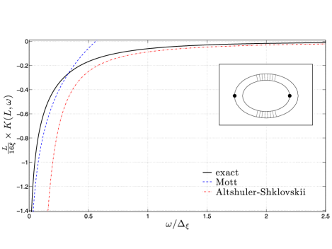
Figure 1: Spectral correlations in a finite-size Anderson insulator, Eqs. (8) and (III.1). For reference we also show previously known limits (dashed lines), i.e. $K(L,\omega)=-(4\xi/L)\left(\Delta_{\xi}/2\omega\right)^{3/2}$ at large, and $K(L,\omega)=-(8\xi/L)\left[\log\left(\Delta_{\xi}/\omega\right)-2\gamma\right]$ at small frequencies respectively, see Eq. (10). Inset: Feynman diagram accounting for Altshuler-Shklovskii correlations Eq. (2); dashed lines represent classical diffusion modes.

III.2 Field-theory

Our derivation of representation (6) starts out from a field-theory description of the level-level correlation function EfetovBook ; altlandfuchs ,

$$K(L,\omega) =-{{\rm Re}\over 32}\int_{0}^{L}dx\int_{0}^{L}dx^{\prime}\,\langle P_{+}[Q(x)]P_{-}[Q(x^{\prime})]\rangle_{Q},$$

$$P_{\pm}[Q] ={\rm str}\left((Q-\Lambda)(1\pm\Lambda)k\right).$$ (11)

Here the average is with respect to the diffusive nonlinear $\sigma$-model action introduced below,

$$\langle...\rangle_{Q} =\int{\cal D}Q\,e^{S_{\sigma}[Q]}.$$ (12)

Integration $\int{\cal D}Q$ is over $4\times 4$ supermatrices $Q(x)=\{Q^{\alpha\alpha^{\prime}}_{ss^{\prime}}(x)\}$ from the supergroup $U(1,1|2)$ obeying the nonlinear constraint $Q^{2}(x)=\openone$. Diagonal $2\times 2$ upper- left and lower-right matrix blocks $Q^{\mathrm{bb}}$ and $Q^{\mathrm{ff}}$, respectively, contain complex numbers. The off-diagonal blocks $Q^{\mathrm{bf,fb}}$ consists of Grassmann variables. The subscript indices $Q_{ss^{\prime}}$, $s,s^{\prime}=\pm$ discriminate between ‘retarded’ and ‘advanced’ components of the matrix field. The $c$-number content of the $Q$-field manifold reduces to the direct product of the hyperboloid $U(1,1)/[U(1)\times U(1)]$ in the ${\rm bb}$-block and the sphere $U(2)/[U(1)\times U(1)]$ in the ${\rm ff}$-block. It is parametrized by non-compact and compact variables, $1\leq\lambda_{\rm bb}$ and $-1\leq\lambda_{\rm ff}\leq 1$, respectively. The matrix $\Lambda=\{s\,\delta_{ss^{\prime}}\}$ is the identity matrix in boson-fermion space but breaks symmetry in advanced-retarded space. $k=\Lambda\sigma_{3}^{\rm bf}$ is a diagonal matrix with $\sigma_{3}^{\rm bf}$ breaking also symmetry in boson-fermion space, and ‘${\rm str}$’ is the generalization of the matrix trace to graded space.

The diffusive nonlinear $\sigma$-model action reads EfetovBook ; EfetovAdv ,

$$S_{\sigma}[Q] =-{\pi\nu S\over 4}\int dx\,{\rm str}\left(2i\omega Q\Lambda+D(\partial_{x}Q)^{2}\right).$$ (13)

It is the low-energy effective field-theory for Anderson localization, here for a quasi one-dimensional geometry and in the presence of a weak time-reversal symmetry breaking vector potential. We refer for a derivation of action (13) to Refs. EfetovBook ; EfetovAdv , and here point out its structural similarity to the Hamilton function of a classical ferromagnet in an external magnetic field. The latter breaks rotational invariance of the exchange interaction, and a similar role is played by the potential $V(Q)\sim{\rm str}\left(Q\Lambda\right)$ in the $\sigma$-model action. $V(Q)$ breaks the invariance of the kinetic term $K(Q)\sim{\rm str}\left([\partial_{x}Q]^{2}\right)$ under general rotations $U(1,1|2)$. The strength of symmetry breaking is given by the level-separation $\omega$. Energies $\omega\gg\Delta_{\xi}$ larger than the level-spacing imply strong symmetry-breaking. $Q$-fields are then pinned to the mean-field $\Lambda$ and small fluctuations can be accounted for perturbatively. A straightforward perturbative expansion at large energies gives the leading correlation function $K(\omega\gg\Delta_{\xi})\propto\omega^{-3/2}$ discussed in the previous section. Once $\omega\lesssim\Delta_{\xi}$ falls below the level-spacing, fluctuations become large acting to restore the full symmetry of the kinetic term. A direct integration of Eq. (III.2) is hindered by the presence of the rotational symmetry breaking potential $V(Q)$. Non-perturbative methods, discussed below, have to be applied to address the low energy correlations $\omega\lesssim\Delta_{\xi}$.

III.3 Non-perturbative solution

We next derive the alternative representation of the correlation function (III.2) in terms of the Green’s function for the Coulomb scattering problem skvortsov . To this end we recall that one can map the integral Eq. (III.2) to a set of equivalent differential equations efetovreview ; EfetovBook . Indeed, identifying $Q$ with the coordinate of a multi-dimensional quantum particle and the wire-coordinate with time, Eq. (13) reads as the Feynman path-integral of a particle with kinetic energy $K(Q)$ moving in the potential $V(Q)$. Alternatively to calculating the path-integral, one can solve the corresponding ‘Schrödinger equation’, known as transfer-matrix equations.

Similar to a radial potential in quantum mechanics, the high degree of symmetry of the potential ($V$ is invariant under similarity transformations of $Q$ leaving $\Lambda$ invariant) reduces the effective dimensionality of the problem. As detailed in Appendix A, correlation function (III.2) reduces to an integral over the $c$-number variables $\lambda_{\rm bb}$ and $\lambda_{\rm ff}$. The integrand is expressed in terms of a ground- and an excited-state wave-function of the underlying Schrödinger equation. As the Laplace-operator on the $Q$-matrix manifold has a rather complex structure closed solutions of the latter are not available.

Progress in this direction has been made in a recent work by Skvortsov and Ostrovsky skvortsov . There the authors elaborate on a connection between localization in quasi one-dimensional systems within the unitary class to scattering in a Coulomb potential. Changing from angle to ‘Coulomb’-coordinates,

$$\lambda_{\rm ff} =(r-r_{1})/2,\quad\lambda_{\rm bb}=(r+r_{1})/2,$$ (14)

a major simplification occurs when the latter are understood as elliptic coordinates of a three-dimensional problem with cylindrical symmetry,

$$r =\sqrt{z^{2}+\rho^{2}},\quad r_{1}=\sqrt{(z-2)^{2}+\rho^{2}}.$$ (15)

Here $(\rho,\varphi,z)$ are the usual cylindrical coordinates. Following the outlined procedure (and leaving details to Appendix B) the correlation function (III.2) becomes

$$K(L,\omega) ={\xi^{2}{\rm Re}\over 2\pi L^{2}}\int_{0}^{L\over\xi}dt^{\prime}\int{d\mathbb{r}\over r}\Phi_{0}(\mathbb{r},L/\xi-t^{\prime})\Phi_{1}(\mathbb{r},t^{\prime}),$$ (16)

where $\Phi_{0}$ and $\Phi_{1}$ are the ground- and excited-state wave-functions, respectively. The latter are solutions of the following transfermatrix equations in Coulomb-coordinates,

$$\left({1\over r_{1}r}\partial_{t}-\partial^{2}_{\mathbb{r}}+{2\kappa\over r}\right)\Phi_{0}(\mathbb{r},t) =0,$$ (17)

$$\left({1\over r_{1}r}\partial_{t}-\partial^{2}_{\mathbb{r}}+{2\kappa\over r}\right)\Phi_{1}(\mathbb{r},t) ={1\over r}\Phi_{0}(\mathbb{r},t).$$ (18)

Here $\partial_{\mathbb{r}}$ is the three-dimensional Laplace operator, $\kappa=\omega/(4i\Delta_{\xi})$ and $t=x/\xi$. Eqs. (17) and (18) are supplemented by the boundary conditions $\Phi_{0}(\mathbb{r},0)=1/r_{1}$ and $\Phi_{1}(\mathbb{r},0)=0$. In the strongly localized regime of interest homogeneous solutions of the transfermatrix equations give the leading contribution to Eq. (16). Indeed, inhomogeneous solutions decay exponentially from the boundaries and their contributions to the integral Eq. (16) can be neglected for $L\gg\xi$. Dropping $t$-dependencies of the wave-functions, Eqs. (17) and (18) become spherical symmetric. The corresponding boundary conditions read $\Phi_{0}(\mathbb{r}_{0})=1/r_{1}$ and $\Phi_{1}(\mathbb{r}_{0})=0$ with $\mathbb{r}_{0}=(0,0,2)^{t}$. The reduction to a problem of higher degree of symmetry is a key simplification which allows for an analytical calculation of (16) to leading order in the small parameter $\xi/L$.

Following Ref. skvortsov, we introduce the zero-energy Green’s function for the non-relativistic $3d$ Coulomb-problem,

$$\left(\partial^{2}_{\mathbb{r}}-{2\kappa\over r}\right)G_{0}(\mathbb{r},\mathbb{r}^{\prime}) =\delta(\mathbb{r}-\mathbb{r}^{\prime}).$$ (19)

Imposing usual boundary condition $G_{0}(\mathbb{r},\mathbb{r}^{\prime})\overset{\mathbb{r}\to\mathbb{r}^{\prime}}{\mapsto}\delta(\mathbb{r}-\mathbb{r}^{\prime})$ the homogeneous solution to Eq. (17) with required boundary condition affords the representation skvortsov

$$\Phi_{0}(\mathbb{r})=-4\pi G_{0}(\mathbb{r},\mathbb{r}_{0}).$$ (20)

Similarly, it is verified that the convolution

$$\Phi_{1}(\mathbb{r})=-\int{d\mathbb{r}^{\prime}\over r^{\prime}}G_{0}(\mathbb{r},\mathbb{r}^{\prime})\Phi_{0}(\mathbb{r}^{\prime})$$ (21)

is a $t$-independent solution of Eq. (18) with the required boundary condition. Inserting above solutions (20) and (21) into (16) one confirms that fn1

$$K(L,\omega) =-{8\pi\xi\over L}{\rm Re}\,\int d\mathbb{r}\int d\mathbb{r}^{\prime}\,G_{0}(\mathbb{r}_{0},\mathbb{r}){1\over r}G_{0}(\mathbb{r},\mathbb{r}^{\prime}){1\over r^{\prime}}G_{0}(\mathbb{r}^{\prime},\mathbb{r}_{0})=-{2\pi\xi\over L}{\rm Re}\,\lim_{\mathbb{r}\to\mathbb{r}_{0}}\partial^{2}_{\kappa}G_{0}(\mathbb{r},\mathbb{r}_{0}).$$ (22)

This completes our derivation of the spectral correlation function (1) in terms of the Green’s function for the Coulomb-scattering problem.

IV From Poisson to Wigner-Dyson statistics

We next address how spectral correlations in a finite-size Anderson insulator turn into Wigner-Dyson correlations as the wire-length is reduced. We recall that in the fully ergodic quantum dot-limit level correlations follow Wigner-Dyson statistics $K(L\to 0,\omega)=-(\Delta/\omega\pi)^{2}\sin^{2}\left(\omega\pi/\Delta\right)$. Here $\Delta=(\nu SL)^{-1}$ is the level spacing of the wire of length $L$. Noting that $\Delta/\Delta_{\xi}\sim\xi/L$, one can thus study how Altshuler-Shklovskii correlations at $\omega\gg\Delta_{\xi}$ evolve into Wigner-Dyson correlations as the wire-length decreases.

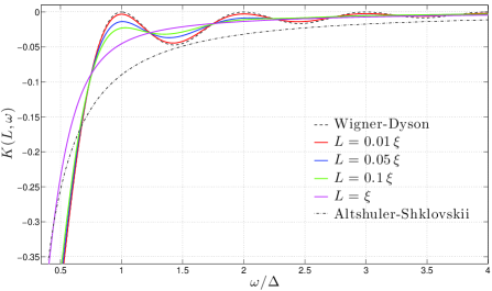
Figure 2: Level-level correlations Eqs. (IV) and (26) for different ratios $L/\xi$ in the Poisson to Wigner-Dyson crossover region. For comparison we also show Wigner-Dyson and Althsuler-Shklovskii correlations (dashed and dashed-dotted lines).

Correlations at arbitrary ratios $L/\xi$ can be derived from the inhomogeneous transfermatrix equations (17) and (18). For levels separated by $\omega\gg\Delta_{\xi}$ the potential $V$ pins the wave-functions to the region $r_{1}\ll 1$ enforced by the boundary conditions. We can thus approximate for the ground-state wave-function

$$\left({1\over 2r_{1}}\partial_{t}-\partial^{2}_{\mathbb{r}}+\kappa\right)\Phi_{0}(\mathbb{r},t) =0.$$ (23)

The radial symmetry of Eq. (23) substantially simplifies the problem. Starting out from the ansatz $\Phi(\mathbb{r},t)=e^{-F(\kappa,t)r_{1}}/r_{1}$ the function $F$ satisfies $\partial_{t}F+2F^{2}-2\kappa=0$. Employing the boundary condition $F(\kappa,0)=0$ one then finds

$$\Phi_{0}(\mathbb{r},t) ={1\over r_{1}}e^{-\sqrt{\kappa}\tanh\left(2\sqrt{\kappa}t\right)r_{1}}.$$ (24)

Eq. (24) interpolates between the known limits at small and large ratios $L/\xi$. Indeed, $\tanh(2\sqrt{\kappa}t)$ approximates to $1$ and $2\sqrt{\kappa}t$ for $\omega/\Delta$ much larger, respectively, smaller than $\xi/L$. This reflects the typical decaying and oscillating behaviors of the ground-state wave-function in the two limits. A similar calculation, detailed in Appendix C, gives for the level-level correlation function

$$K(L,\omega) ={\Delta\xi\,{\rm Im}\over\pi L}\,\int_{0}^{L\over\xi}dt^{\prime}\,\left(1-e^{-H^{-1}(\omega/i\Delta_{\xi},L/\xi,t^{\prime})}\right)$$

$$\qquad\qquad\qquad\times\partial_{\omega}H(\omega/i\Delta_{\xi},L/\xi,t^{\prime}),$$ (25)

with

$$H(z,t,t^{\prime}) ={\cosh(\sqrt{z}t^{\prime})\cosh(\sqrt{z}(t^{\prime}-t))\over\sqrt{z}\sinh(\sqrt{z}t)}.$$ (26)

We emphasize that Eqs. (IV), (26) hold for $\omega\gg\Delta_{\xi}$ and arbitrary ratios $L/\xi$.

The analytical result (IV), (26) is displayed in Fig. 2. It shows how the Altshuler-Shklovskii correlations in long wires evolve into the Wigner-Dyson correlations as one approaches the quantum-dot limit. Unfortunately, we do not know the corresponding result for correlations between levels separated by $\omega\lesssim\Delta_{\xi}$. The transfermatrix equations in the Poisson-to-Wigner-Dyson crossover region then lack rotational symmetry and we were not able to find analytical solutions.

V Summary and discussion

In this paper we have derived the leading level-level correlations in quasi one-dimensional Anderson insulators with broken time-reversal symmetry. While energy levels are uncorrelated in the thermodynamic limit correlations remain in finite-size Anderson insulators.

The correlations of far-distant and nearby levels reflect the dynamics in the classical diffusive regime and the deep quantum regime of strong Anderson localization. They have been well-established for decades AltshulerShklovskii ; altlandfuchs . This paper discusses the previously unknown correlations at arbitrary level-separations. Specifically, our result describes how Altshuler-Shklovskii correlations at large separations turn into logarithmic level-repulsion at small separations. Only in the limit of infinite wire-length the correlations vanish, in accordance with universal Poisson statistics expected in the non-ergodic system.

We further discuss how Altshuler-Shklovskii correlations in Anderson insulators turn into Wigner-Dyson correlations with decreasing wire-length. A corresponding analysis for correlations between close-by levels remains an open problem.

Finally, we would like to put our results into the context of previous works. Spectral correlations of quasi one-dimensional disordered systems in the Wigner-Dyson-to-Poisson crossover have been addressed in Ref. altlandfuchs, . From numerical solutions of the relevant transfermatrix equations a qualitative understanding of the level-level correlation function in the Wigner-Dyson-to-Poisson crossover was obtained. Local correlations in the density of states within a localization volume were derived in Ref. skvortsov, . The authors find the exact ground-state wave-function of the homogeneous transfermatrix equation by mapping the equation to the Coulomb-scattering problem. It is shown that correlations of different eigenfunctions are different in quasi- and strictly one-dimensional geometries 1dchain . Correlation functions for the global density of states (discussed in this work) and the local density of states (discussed in Ref. skvortsov, ) both have representations in terms of the Coulomb Green’s function. A similar relation has been observed in Ref. altshulerlg, in the context of parametric correlations, where it was connected to a symmetry in the $\sigma$-model. Ref. Ivanov2009, derives a perturbative expansion for the local density of states correlation function at small frequencies. Their general expression e.g. reproduces statistics of single localized wave-functions and predicts re-entrant behavior at the Mott scale (similar to that in strictly $1d$ chains 1dchain ). It would be interesting to investigate how the findings reported in the present work are obtained within this approach. Furthermore, extensions of the discussed results to other symmetry classes remains an open problem.

Appendix A Transfermatrix equations

For self-consistency we state the level-level correlation function in a quasi one-dimensional wire. In the unitary symmetry class the latter depends on the $c$-number variables $\lambda_{\rm bb}$, $\lambda_{\rm ff}$. Following Refs. EfetovBook, ; efetovreview, ; altlandfuchs, one finds

$$K(L,\omega) ={\xi^{2}\over L^{2}}{\rm Re}\int_{0}^{L\over\xi}dt^{\prime}\int_{1}^{\infty}{d\lambda_{1}}\int_{-1}^{1}{d\lambda\over\lambda_{1}-\lambda}$$

$$\qquad\times\,\Psi_{0}(\lambda_{1},\lambda,L/\xi-t^{\prime})\Psi_{1}(\lambda_{1},\lambda,t^{\prime}).$$ (27)

For notational convenience we here introduced $\lambda_{\rm bb}\equiv\lambda_{1}$ and $\lambda_{\rm ff}\equiv\lambda$, and $\Psi_{0}$ and $\Psi_{1}$ are the ground-state and an excited-state wave-function, respectively. The latter follow the transfermatrix equations

$$\left(\partial_{t}+2\hat{H}_{0}\right)\Psi_{0}(\lambda_{1},\lambda,t) =0,$$ (28)

$$\left(\partial_{t}+2\hat{H}_{0}\right)\Psi_{1}(\lambda_{1},\lambda,t) =(\lambda_{1}-\lambda)\Psi_{0}(\lambda_{1},\lambda,t),$$ (29)

where we introduced $t=x/\xi$. The Hamilton operator reads $\hat{H}_{0}=\Delta_{Q}+\hat{V}$, where

$$\Delta_{Q} =-{(\lambda_{1}-\lambda)^{2}\over 2}\left(\partial_{\lambda}{1-\lambda^{2}\over(\lambda_{1}-\lambda)^{2}}\partial_{\lambda}+\partial_{\lambda_{1}}{\lambda_{1}^{2}-1\over(\lambda_{1}-\lambda)^{2}}\partial_{\lambda_{1}}\right)$$ (30)

is the Laplace operator on the $Q$-field manifold, and

$$\hat{V} =-{i\omega\over 4\Delta_{\xi}}(\lambda_{1}-\lambda),$$ (31)

is the symmetry-breaking potential. The above equations should be solved with boundary conditions for an open wire,

$$\Psi_{0}(\lambda_{1},\lambda,0)=1,\qquad\Psi_{1}(\lambda_{1},\lambda,0)=0.$$ (32)

Appendix B Cylindrical coordinates

Employing elliptic coordinates ($\lambda_{\rm bb}\equiv\lambda_{1}$, $\lambda_{\rm ff}\equiv\lambda$)

$$\lambda =(r-r_{1})/2,\quad\lambda_{1}=(r+r_{1})/2,$$ (33)

$$r =\sqrt{z^{2}+\rho^{2}},\quad r_{1}=\sqrt{(z-2)^{2}+\rho^{2}},$$ (34)

the Hamilton operator takes the form

$$\hat{H}_{0} =-{r_{1}^{2}r\over 2}\left[\partial_{z}^{2}+\partial_{\rho}^{2}+{1\over\rho}\partial_{\rho}+{i\omega\over 2\Delta_{\xi}r}\right]{1\over r_{1}}.$$ (35)

Notice that the differential operator is the usual Laplacian in cylindrical coordinates $(\rho,\varphi,z)$, acting on cylindrical symmetric functions.

It is then convenient to make the ansatz $\Psi_{i}=r_{1}\Phi_{i}$ and to express the corresponding Schrödinger equations in three-dimensional coordinates

$$\left(\partial_{t}-r_{1}r\partial^{2}_{\mathbb{r}}+2r_{1}\kappa\right)\Phi_{0}(\mathbb{r},t) =0,$$ (36)

$$\left(\partial_{t}-r_{1}r\partial^{2}_{\mathbb{r}}+2r_{1}\kappa\right)\Phi_{1}(\mathbb{r},t) =r_{1}\Phi_{0}(\mathbb{r},t).$$ (37)

Here $\kappa=\omega/(4i\Delta_{\xi})$ and we recall that the boundary conditions read $\Phi_{0}(\mathbb{r},0)=1/r_{1}$ and $\Phi_{1}(\mathbb{r},0)=0$. The integration measure transforms into the three-dimensional volume element of cylindrical symmetric functions,

$$d\lambda\wedge d\lambda_{1} ={\rho\over rr_{1}}dz\wedge d\rho\mapsto{d\mathbb{r}\over 2\pi rr_{1}},$$ (38)

where $d\mathbb{r}=dz\wedge\rho d\rho\wedge d\varphi$. The level-level correlation function thus takes the form

$$K(L,\omega) ={\xi^{2}{\rm Re}\over 2\pi L^{2}}\int_{0}^{L\over\xi}dt^{\prime}\int{d\mathbb{r}\over r}\Phi_{0}(\mathbb{r},L/\xi-t^{\prime})\Phi_{1}(\mathbb{r},t^{\prime}).$$ (39)

Appendix C Poisson-to-Wigner-Dyson crossover

Level-level correlations in systems of arbitrary ratios $L/\xi$ can be derived from the inhomogeneous transfermatrix equations. For levels separated by $\omega\gg\Delta_{\xi}$ the potential $V$ pins the ground state wave-function to the region $r_{1}\ll 1$ enforced by the boundary condition. We may thus approximate Eq. (17) by

$$\left(\partial_{t}-2r_{1}\partial^{2}_{\mathbb{r}}+2r_{1}\kappa\right)\Phi_{0}(\mathbb{r},t) =0.$$ (40)

Eq. (40) with boundary condition $\Phi_{0}(\mathbb{r},0)=1/r_{1}$ is solved by $\Phi_{0}(\mathbb{r},t)=e^{-\sqrt{\kappa}\tanh\left(2\sqrt{\kappa}t\right)r_{1}}/r_{1}$. Similarly, one may verify that for $\omega\gg\Delta_{\xi}$ the excited-state wave-function

$$\Phi_{1}(\mathbb{r},t) =-{1\over 2}\partial_{\kappa}\Phi_{0}(\mathbb{r},t)$$ (41)

satisfies transfermatrix equation

$$\left(\partial_{t}-2r_{1}\partial^{2}_{\mathbb{r}}+2r_{1}\kappa\right)\Phi_{1}^{0}(\mathbb{r},t) =r_{1}\Phi_{0}(\mathbb{r},t),$$ (42)

with boundary condition $\Phi_{1}(\mathbb{r},0)=0$. Inserting $\Phi_{0}$ and $\Phi_{1}$ into the level-level correlation function (39) one arrives at Eqs. (26) and (IV) stated in the main text. Notice that in the quantum-dot limit $\Phi_{0}(\mathbb{r},t)=e^{-2\kappa r_{1}t}/r_{1}$ and $\Phi_{1}(\mathbb{r},t)=te^{-2\kappa r_{1}t}$. This results in the Wigner-Dyson correlations $K(L,\omega)=-(\Delta/\omega\pi)^{2}\sin^{2}(\omega\pi/\Delta)$ applicable at arbitrary ratios $\omega/\Delta$. That is, the restriction $\omega\gg\Delta_{\xi}\sim\Delta L/\xi$ becomes irrelevant in the limit $L\ll\xi$.

References

- (1) F. Haake, Quantum Signatures of Chaos, (Springer, 2010).
- (2) N. F. Mott, Philos. Mag. 22, 7 (1970).
- (3) L. P. Gor kov, O. N. Dorokhov, and F. V. Prigara, Sov. Phys. JETP 57, 838 (1983).
- (4) U. Sivan and Y. Imry, Phys. Rev. B 35, 6074 (1987).
- (5) For a recent reconsideration of Mott’s argument, see D. A. Ivanov, M. A. Skvortsov, P. M. Ostrovsky, and Ya. V. Fominov, Phys. Rev. B 85, 035109 (2012).
- (6) K. B. Efetov, Supersymmetry in Disorder and Chaos (Cambridge University Press, 1999).
- (7) K. B. Efetov, Adv. Phys. 32, 53 (1983).
- (8) O. Bohigas, M. J. Giannoni, and C. Schmit, Phys. Rev. Lett. 52, 1 (1984).
- (9) M. V. Berry, Ann. Phys. (N.Y.) 131, 163 (1981).
- (10) S. Müller, S. Heusler, P. Braun, F. Haake, and A. Altland, Phys. Rev. Lett. 93, 014103 (2004).
- (11) S. Müller, S. Heusler, P. Braun, F. Haake, and A. Altland, Phys. Rev. E 72 , 046207 (2005).
- (12) S. Heusler, S. Müller, A. Altland, P. Braun, and F. Haake, Phys. Rev. Lett. 98, 044103 (2007).
- (13) B. L. Altshuler, B. I. Shklovskii, JETP 64, 127 (1986).
- (14) A. Altland and D. Fuchs, Phys. Rev. Lett. 74, 4269 (1995).
- (15) M. A. Skvortsov and P. M. Ostrovsky, JETP Lett. 85, 72 (2007).
- (16) L. Hostler and R. H. Pratt, Phys. Rev. Lett 10, 469 (1963).
- (17) L. Hostler, J. Math. Phys. 5, 591 (1964).
- (18) I. S. Gradsteyn and I. M. Ryzhik, Table of integrals, series, and products (Academic Press, New York, 2000).
- (19) K. B. Efetov and A. Larkin, Sov. Phys. JETP 58, 444 (1983).
- (20) We anticipate symmetry in the arguments of the Green’s function, , evident in Eq. (7).
- (21) N. Taniguchi, B. D. Simons, and B. L. Altshuler. Phys. Rev. B 53, R7618(R) (1996).
- (22) D. A. Ivanov, P. M. Ostrovsky, and M. A. Skvortsov, Phys. Rev. B 79, 205108 (2009).