On Nambu’s Fermion-Boson Relations for Superfluid ³He

Abstract

Superfluid ³He is a spin-triplet ($S=1$), p-wave ($L=1$) BCS condensate of Cooper pairs with total angular momentum $J=0$ in the ground state. In addition to the breaking of ${\tt U(1)}_{\mbox{\footnotesize\negthinspace}}$ gauge symmetry, separate spin or orbital rotation symmetry is broken to the maximal sub-group, ${\tt SO(3)_{\text{S}}}\times{\tt SO(3)_{\text{L}}}\rightarrow{\tt SO(3)}_{\mbox{\footnotesize\text{J}}}$. The Fermions acquire mass, $m_{\text{F}}\equiv\Delta$, where $\Delta$ is the BCS gap. There are also 18 Bosonic excitations - 4 Nambu-Goldstone (NG) modes and 14 massive amplitude Higgs (AH) modes. The Bosonic modes are labeled by the total angular momentum, $J\in\{0,1,2\}$, and parity under particle-hole symmetry, $c=\pm 1$. For each pair of angular momentum quantum numbers, $J,J_{z}$, there are two Bosonic partners with $c=\pm 1$. Based this spectrum Nambu proposed a sum rule connecting the Fermion and Boson masses for BCS type theories, which for ³He-B is $M_{\text{$J,+$}}^{2}+M_{\text{$J,-$}}^{2}=4m_{\text{F}}^{2}$ for each family of Bosonic modes labeled by $J$, where $M_{\text{$J,c$}}$ is the mass of the Bosonic mode with quantum numbers $(J,c)$. Nambu’s sum rule (NSR) has recently been discussed in the context of Nambu-Jona-Lasinio models for physics beyond the standard model to speculate on possible partners to the recently discovered Higgs Boson at higher energies. Here we point out that Nambu’s Fermion-Boson mass relations are not exact. Corrections to the Bosonic masses from (i) leading order strong-coupling corrections to BCS theory, and (ii) polarization of the parent Fermionic vacuum lead to violations of the sum-rule. Results for these mass corrections are given in both the $T\rightarrow 0$ and $T\rightarrow T_{c}$ limits. We also discuss experimental results, and theoretical analysis, for the masses of the $J^{\mbox{\small c}}=2^{\pm}$ Higgs modes and the magnitude of the violation of the NSR.

I Introduction

One of the key features of spontaneous symmetry breaking in condensed matter and quantum field theory is the emergence of new elementary quanta - phonons in crystalline solids, magnons in ferromagnets, the Higgs and gauge bosons of the standard model. In the latter example, spontaneous symmetry breaking (SSB) in the BCS theory of superconductivity played an important role in theoretical models for the mass spectrum of elementary particles.Nambu and Jona-Lasinio (1961); Anderson (1963); Higgs (1964) In BCS superfluids the binding of Fermions into Cooper pairs leads to an energy gap, $\Delta$, in the Fermion spectrum, i.e. Fermions in the broken symmetry phase (Bogoliubov quasiparticles) acquire a mass $m_{\text{F}}=\Delta$, while condensation of Cooper pairs leads to the breaking of global ${\tt U(1)}_{\mbox{\footnotesize\negthinspace}}$ gauge symmetry, the generator being particle number. The latter also implies that the Bogoliubov Fermions are no longer particle number (Fermion “charge”) eigenstates, but coherent superpositions of normal-state particles and holes. Charge conservation is ensured by an additional contribution to the charge current - a collective mode of the broken symmetry phase. This massless Bosonic excitation of the phase of condensate amplitudeAnderson (1958a); Bogoliubov (1958) is the Nambu-Goldstone (NG) mode associated with broken ${\tt U(1)}_{\mbox{\footnotesize\negthinspace}}$ symmetry, and is manifest as a phonon in neutral superfluid ³He.

II Nambu’s Mass Relations

Nambu and Jona-Lasinio’s development of a dynamical theory for the masses of elementary particles Nambu and Jona-Lasinio (1961) was influenced by the BCS theory of superconductivity, and particularly Bogoliubov Bogoliubov (1958), Valatin Valatin (1958) and Anderson’s Anderson (1958b, 1963) contributions on the excitation spectrum of Fermions and the collective excitations (Bosonic) associated with broken gauge symmetry.Nambu (2009) BCS-type theories, including the NJL theory, imply a connection between the masses of the emergent Fermionic and Bosonic excitations. In the case of conventional BCS theory there are two Bosonic modes - the phase mode and the amplitude mode with mass $M_{\text{H}}=2\Delta$. The phase mode, discussed independently by Anderson and Bogoliubov, is the massless NG mode ($M_{\text{NG}}=0$), while the amplitude mode is the Higgs Boson of BCS theory.Higgs (1964); Littlewood and Varma (1981) This doubling of the Bosonic spectrum reflects a discrete symmetry under charge conjugation, $C$, (i.e. “particle $\leftrightarrow$ hole” symmetry) of the symmetry un-broken Fermionic vacuum,Serene (1983); Sauls and McKenzie (1991) and is characteristic of spontaneous symmetry breaking of the BCS type, including BCS systems with more complex symmetry breaking phase transitions. In particular, the amplitude (phase) mode has even (odd) parity with respect to charge conjugation.Serene (1983) Furthermore, the masses of the Fermions and the Bosons obey the sum rule $M_{\text{NG}}^{2}+M_{\text{H}}^{2}=(2m_{\text{F}})^{2}$.

Nambu argued that similar sum rules apply to a broad class of BCS type theories - from nuclear structure and QCD to exotic pairing in condensed matter systems - that exhibit complex symmetry breaking.Nambu (1985) The ground state of superfluid ³He provides the paradigm. Superfluid ³He-B is a condensate of p-wave ($L=1$), spin-triplet ($S=1$) Cooper pairs with total angular momentum $J=0$. Thus, in addition to the breaking of ${\tt U(1)}_{\mbox{\footnotesize\negthinspace}}$, the symmetry of the normal quantum liquid with respect to separate spin or orbital rotations is broken to the maximal sub-group, ${\tt SO(3)_{\text{S}}}\times{\tt SO(3)_{\text{L}}}\rightarrow{\tt SO(3)}_{\mbox{\footnotesize\text{J}}}$. The Fermion spectrum is isotropic and gapped with mass determined by the binding energy of Cooper pairs, $m_{\text{F}}=\Delta$. However, there are now 18 Bosonic excitations - 4 NG modes and 14 massive Higgs modes. The Bosonic modes are organized into six multiplets labeled by $J^{\mbox{\small c}}$ - total angular momentum, $J\in\{0,1,2\}$, and parity under charge conjugation (particle $\leftrightarrow$ hole), $\mbox{\small c}=\pm 1$. For each $J$ there are $2J+1$ degenerate states with angular momentum projection $m=-J,\ldots,+J$, and for each pair of values of $J,m$ there are two Bosonic modes with $\mbox{\small c}=\pm 1$.

The $J=0$ modes are the NG mode associated with broken ${\tt U(1)}_{\mbox{\footnotesize\negthickspace}}$ symmetry ($J^{\mbox{\small c}}=0^{-}$) and the Higgs mode ($J^{\mbox{\small c}}=0^{+}$), which has the same quantum numbers as the B-phase vacuum, i.e. the condensate of ground state Cooper pairs. There are six $J=1$ modes: 3 NG modes ($J^{\mbox{\small c}}=1^{+}$) corresponding to the degeneracy of the B-phase ground state with respect to relative spin-orbit rotations, and 3 Higgs modes ($J^{\mbox{\small c}}=1^{-}$) with masses $M_{1,-}=2\Delta$.McKenzie and Sauls (1993) Finally, there are ten modes with $J=2$, all of which are Higgs modes with masses $M_{2,\pm}<2\Delta$, with original calculations giving $M_{2,+}=\sqrt{\frac{2}{5}}\,\,2\Delta$ and $M_{2,-}=\sqrt{\frac{3}{5}}\,\,2\Delta$.Vdovin (1963); Maki (1974); Wölfle (1976); Brusov and Popov (1980) Nambu noted that all three multiplets obey a sum rule connecting the masses of the conjugate Bosonic modes and the Fermionic mass,Nambu (1985)

$$M_{J,+}^{2}+M_{J,-}^{2}=(2m_{\text{F}})^{2}\,,\quad J\in\{0,1,2\}\,,$$ (1)

and suggested that such Fermion-Boson relations are generic to BCS-type NJL models in which both Fermion and Boson excitations originate from interactions between massless progenitor Fermions and spontaneous symmetry breaking (see also Ref. Volovik and Zubkov, 2013). Nambu further speculated that these Fermion-Boson mass relations reflected a hidden supersymmetry in class of BCS-NJL models,Nambu (1985) and in the case of of conventional s-wave, spin-singlet BCS superconductivity was able to construct a supersymmetric representation for the static part of the effective Hamiltonian, $H_{\mbox{s}}$, and identify the superalgebra as ${\tt su(2/1)}_{\mbox{\footnotesize\negthinspace}}$. The Fermion operators in Nambu’s construction factorize $H_{\mbox{s}}$, and provide ladder operators connecting the Fermionic and Bosonic sectors of the spectrum, and generate the Fermion-Boson mass relations: $M_{\text{NG}}=0$, $m_{\text{F}}=\Delta$, and $M_{\text{H}}=2\Delta$.Nambu (1995)^,

Recently, Volovik and Zubkov argued that the Nambu sum rule (NSR) for ³He-B follows from the symmetry of the B-phase vacuum and the quantum numbers $(J,m)$ (c.f. Sec. 2.2 of Ref. Volovik and Zubkov, 2014). Based on the NSR for a NJL-type theory of top quark condensation, the authors suggest the possibility that there may be a partner to the Higgs Boson with a mass of $125\,\mbox{GeV}$ - e.g. a Higgs partner near $270\,\mbox{GeV}$,Volovik and Zubkov (2013, 2014) analogous to the Higgs partners for the $J=2$ Bosonic spectrum of ³He-B. Here we point out that estimates of the mass of a Higgs partner based on such sum rules may be imprecise because the NSR is generally violated. The origins of the violation of the NSR contain detailed information about the parent Fermionic vacuum. While one might expect that the masses for the $J$ multiplets to be protected by the residual symmetry of the broken-symmetry vacuum state, it is generally not the case. As a result the NSR is not exact, particularly for BCS-type theories with multiplets of NG and Higgs Bosons with quantum numbers that are distinct from that of the broken symmetry vacuum state. We discuss the violations of the NSR for the case of ³He-B in two limits: (i) time-dependent Ginzburg-Landau (TDGL) theory appropriate for $T\lesssim T_{c}$ and (ii) a dynamical theory for coupled Fermionic and Bosonic excitations of ³He-B within the BCS theory for p-wave, spin-triplet pairing (i.e. one-loop approximation to the self-energy) for temperature $T\rightarrow 0$. In particular, interactions between the progenitor Fermions, combined with vacuum polarization, lead to mass shifts of the Higgs modes whose quantum numbers differ from the broken symmetry vacuum state, e.g. the $J^{\mbox{\small c}}=1^{\pm}$ and $J^{\mbox{\small c}}=2^{\pm}$ modes of ³He-B, and thus to violations of the Nambu sum rule. Explicit results for these mass corrections are derived in both the $T\rightarrow 0$ and $T\rightarrow T_{c}$ limits.

In Secs. III and IV we introduce a Lagrangian for the Bosonic modes of a spin-triplet, p-wave BCS condensate based on a time-dependent extension of Ginzburg-Landau theory (TDGL). This allows us to identify and calculate the Bosonic spectrum for ³He, and to quantify strong-coupling corrections to the Bosonic masses in the limit $T\rightarrow T_{c}$. In particular, strong-coupling feedback (i.e. next-to-leading order loop corrections) leads to mass shifts, and thus violations of the NSR. We also obtain a formula for the mass of the $J^{\mbox{\small c}}=2^{-}$ mode in the GL limit that could provide a direct determination of the GL strong-coupling parameter $\beta_{1}$ from measurements of the $J^{\mbox{\small c}}=2^{-}$ mode via ultrasound spectroscopy.

At low temperatures strong-coupling feedback corrections are suppressed. However in Sec. V we show that vacuum polarization and four-Fermion interactions, in both the particle-hole (Landau) and the particle-particle (Cooper) channels, lead to substantial mass corrections for $T\ll T_{c}$, and in some cases strong violations of the NSR. We discuss experimental measurements for the masses of the $J^{\mbox{\small c}}=2^{\pm}$ modes, and compare the observed mass shifts with theoretical calculations of the polarization corrections to the masses from interactions in the Landau and Cooper channels.

III Ginzburg-Landau Functional

We start from a Ginzburg-Landau (GL) functional applicable to p-wave, spin-triplet pairing beyond the weak-coupling BCS limit, and use this formulation to obtain an effective Lagrangian for the Bosonic fluctuations of superfluid ³He-B in the strong-coupling limit. The GL theory for superfluid ³He was developed by several authors.Mermin and Stare (1973); Brinkman and Anderson (1973); Leggett (1975) We follow the notation Ref. Rainer and Serene, 1976 which provides the bridge between the GL theory and the microscopic theory of leading order strong-coupling effects. The order parameter is identified with the mean-field pairing self-energy, $\hat{\Delta}({\bf p})$, which is a $2\times 2$ matrix of the spin components of the pairing amplitude. For p-wave, spin-triplet condensates the order parameter is symmetric in spin-space, $\hat{\Delta}({\bf p})=(i\sigma_{\alpha}\sigma_{y})\,A_{\alpha i}\,(\hat{\bf p})_{i}$, and parametrized by a $3\times 3$ complex matrix, $A_{\alpha i}$, that transforms as a vector with respect to index $\alpha=\{x^{\prime},y^{\prime},z^{\prime}\}$ under spin rotations, and, separately, as a vector with respect to index $i=\{x,y,z\}$ under orbital rotations. This representation for the order parameter provides us with a basis for an irreducible representation of the maximal symmetry group of normal ³He, ${\mathsf{G}}={\tt SO(3)_{\text{S}}}\times{\tt SO(3)_{\text{L}}}\times{\tt U(1)_{\text{N}}}\times{\tt P}\times{\tt T}$. The GL free energy functional is then constructed from products of $A_{\alpha i}$ and its derivatives, $\partial_{j}A_{\alpha i}$, that are invariant under ${\mathsf{G}}$. The general form for the GL functional for the condensation energy and gradient energy is

$${\cal F}[A]=\int_{V}dV\,\{U(A)+W(\partial A)\}\,,$$ (2)

where

$$U\negthickspace\negthickspace = \negthickspace\negthickspace\alpha(T)\,Tr\left(AA^{\dagger}\right)\negthickspace+\beta_{1}\left|Tr(AA^{T})\right|^{2}\negthickspace+\beta_{2}\left[Tr(AA^{\dagger})\right]^{2}$$

$$+ \negthickspace\negthickspace\beta_{3}Tr\left[AA^{T}(AA^{T})^{*}\right]\negthickspace\negthinspace+\beta_{4}Tr\left[(AA^{\dagger})^{2}\right]\negthickspace\negthinspace+\beta_{5}Tr\left[AA^{\dagger}(AA^{\dagger})^{*}\right]\,.$$

are the six invariants for the condensation energy density, and

$$W\negthickspace=\negthickspace K_{1}\partial_{j}A_{\alpha i}\partial_{j}A_{\alpha i}^{*}\negthickspace+K_{2}\partial_{i}A_{\alpha i}\partial_{j}A_{\alpha j}^{*}\negthickspace+K_{3}\partial_{j}A_{\alpha i}\partial_{i}A_{\alpha j}^{*}\,,$$ (4)

are the three second-order invariants for the gradient energy.

Weak-coupling BCS theory can be formulated at all temperatures in terms of a stationary functional of $\hat{\Delta}({\bf p})$,Serene and Rainer (1983); Ali et al. (2011) which depends on material parameters of the parent Fermionic ground state: $N(0)=k_{f}^{3}/2\pi^{2}\,v_{f}p_{f}$ is the single-spin quasiparticle density of states at the Fermi surface, expressed in terms of the Fermi velocity, $v_{f}$, Fermi momentum and Fermi wave number, $p_{f}=\hbar k_{f}$. The GL limit of the weak-coupling functional can be expressed in the form of Eqs. III and 4 with the following material parameters,

$$\alpha(T) = \frac{1}{3}N(0)(T/T_{c}-1)\,,\quad\beta^{\text{wc}}_{1}\equiv\frac{7\zeta(3)}{240}\frac{N(0)}{(\pi k_{\text{B}}T_{c})^{2}}\,,$$ (5)

$$2\beta^{\text{wc}}_{1} = -\beta^{\text{wc}}_{2}=-\beta^{\text{wc}}_{3}=-\beta^{\text{wc}}_{4}=+\beta^{\text{wc}}_{5}=-2\beta_{\text{wc}}\,.$$ (6)

Strong-coupling corrections to the weak-coupling GL $\beta$ parameters based on the leading-order expansion of Rainer and SereneRainer and Serene (1976) were calculated and reported in Ref. Sauls and Serene, 1981a for quasiparticle scattering that is dominated by ferromagnetic spin fluctuation exchange. The results for the strong-coupling corrections to the weak-coupling $\beta^{\text{wc}}_{i}$ are extrapolated to all pressures as shown in Fig. 1, with $p=0\,\mbox{bar}$ corresponding to weak-coupling.

The weak-coupling form of the gradient energy in Eq. 4 is similarly obtained with the gradient coefficients given by

$$K^{\text{wc}}_{1} = K^{\text{wc}}_{2}=K^{\text{wc}}_{3}=\frac{1}{5}N(0)\,\xi_{\text{GL}}^{2}\,,$$ (7)

$$\xi_{\text{GL}} = \sqrt{\frac{7\zeta(3)}{12}}\frac{\hbar v_{f}}{2\pi k_{B}T_{c}}\,.$$ (8)

The Cooper pair correlation length, $\xi_{\text{GL}}$, varies from $\xi_{\text{GL}}\simeq 650$ Å at $p=0\,\mbox{bar}$ to $\xi_{\text{GL}}\simeq 150$ Å at $p=34\,\mbox{bar}$.

The Balian-Werthamer (BW) state defined by

$$A^{\text{BW}}_{\alpha i}=\frac{\Delta}{\sqrt{3}}\,e^{i\varphi}R[\vec{\vartheta}]_{\alpha i}\,,$$ (9)

where $R[\vec{\vartheta}]$ is an orthogonal matrix, minimizes the GL functional for $\Delta^{2}=-\alpha(T)/2\beta_{\text{B}}$, with $\beta_{\text{B}}=\beta_{12}+\frac{1}{3}\beta_{345}$, in the weak-coupling limit, $\beta^{\text{wc}}_{\text{B}}=\genfrac{}{}{}{1}{5}{6}\beta^{\text{wc}}$, and for all pressures $P<P_{\text{PCP}}\approx 21\,\mbox{bar}$. Note that the amplitude of the order parameter, $\Delta$, is fixed at the minimum of the effective potential. However, the phase, $\varphi$, and the orthogonal matrix, $R[\vec{\vartheta}]$, parametrized by a rotation angle $\vartheta$ about an axis of rotation, $\hat{\bf n}$, define the degeneracy space of the B-phase. In particular,

$$B_{\alpha i}\equiv\frac{\Delta}{\sqrt{3}}\,\delta_{\alpha i}\,,$$ (10)

corresponding to pairs with $L=1$, $S=1$ and $J=0$ is degenerate with states obtained by any relative rotation, $R[\vec{\vartheta}]$, of the spin and orbital coordinates combined with a gauge transformation, $e^{i\varphi}$. Since the GL functional defined by Eqs. III and 4 is invariant under these operations we can use the $J=0$ BW state as the reference ground state.

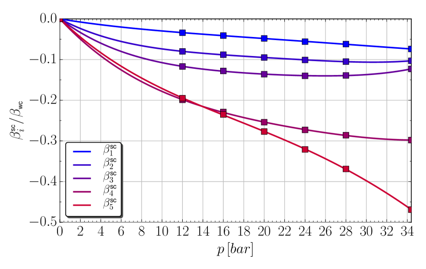
Figure 1: Strong-coupling corrections ($\beta^{\text{sc}}_{i}\equiv\beta_{i}-\beta^{\text{wc}}_{i}$) to the GL $\beta$ parameters interpolated from the results of Ref. Sauls and Serene, 1981a [data squares]. The $\beta^{\text{sc}}_{i}$ are extrapolated below $P=12$ bar to weak-coupling ($\beta^{\text{sc}}_{i}=0$) at $p=0$ bar.

IV Time Dependent GL Theory

Bosonic excitations of the BW ground state are represented by space-time fluctuations of the pairing amplitude: ${\mathcal{D}}_{\alpha i}({\bf r},t)=A_{\alpha i}({\bf r},t)-B_{\alpha i}$. The potential energy for these fluctuations is obtained by expanding the GL functional to 2^nd order in the fluctuations ${\mathcal{D}}({\bf r},t)$: ${\cal U}[{\mathcal{D}}]={\cal F}[A]-{\cal F}[B]$.Volovik and Khazan (1984); Theodorakis (1988) Time-dependent fluctuations, $\dot{{\mathcal{D}}_{\alpha i}}=\partial_{t}{\mathcal{D}}_{\alpha i}$, lead to an additional invariant, ${\cal K}=\tau\int_{\text{V}}dV\,\dot{\mathcal{D}}_{\alpha i}\dot{\mathcal{D}}_{\alpha i}^{*}$, where $\tau$ is the effective inertia for Cooper pair fluctuations. The Lagrangian for the Bosonic excitations, ${\cal L}={\cal K}-{\cal U}$, takes the form,

$${\cal L}\negthickspace=\negthickspace\negthickspace\int\negthickspace\negthinspace dV\negthickspace \Bigg{\{} \negthickspace\tau\,\mbox{Tr}\Big{\{}\dot{\mathcal{D}}\dot{\mathcal{D}}^{{\dagger}}\Big{\}}\negthinspace-\negthinspace\alpha\,\mbox{Tr}\Big{\{}{\mathcal{D}}{\mathcal{D}}^{{\dagger}}\Big{\}}\negthinspace-\negthinspace\sum_{p=1}^{5}\beta_{p\,}u_{p}({\mathcal{D}})$$ (11)

$$\negthinspace-\negthinspace \sum_{l=1}^{3}\,K_{l}\,v_{l}(\partial{\mathcal{D}})\negthinspace-\negthinspace\left(\eta_{\alpha i}{\mathcal{D}}_{\alpha i}^{*}+\eta_{\alpha i}^{*}{\mathcal{D}}_{\alpha i}\right)\negthickspace\Bigg{\}}\,.$$

The terms $u_{p}({\mathcal{D}})$ are the effective potentials corresponding to fluctuations, ${\mathcal{D}}$, relative to the BW ground state, which to quadratic order in ${\mathcal{D}}$ are given in Eqs. 114-118 of the Appendix. The terms, $w_{l}(\partial{\mathcal{D}})$, are obtained from Eq. 4 with $A\rightarrow{\mathcal{D}}$, and the last pair of terms in Eq. 11 represent an effective external source potential for Cooper pair fluctuations.

The Euler-Lagrange equations,

$$\mbox{$\displaystyle\frac{\delta{\cal L}}{\delta{\mathcal{D}}_{\alpha i}^{*}}$}-\mbox{$\displaystyle\frac{\partial}{\partial t}$}\mbox{$\displaystyle\frac{\delta{\cal L}}{\delta\dot{\mathcal{D}}_{\alpha i}^{*}}$}-\mbox{$\displaystyle\frac{\partial}{\partial x_{j}}$}\mbox{$\displaystyle\frac{\delta{\cal L}}{\delta\partial_{j}{\mathcal{D}}_{\alpha i}^{*}}$}=0\,,$$ (12)

reduce to field equations for the Cooper-pair fluctuations,

$$\tau\ddot{\mathcal{D}}_{\alpha i}\negthickspace-\negthickspace|\alpha|{\mathcal{D}}_{\alpha i}\negthinspace+\negthinspace\Delta^{2}\negthinspace\sum_{a=1}^{5}\negthinspace\beta_{a}\,\mbox{$\displaystyle\frac{\partial\bar{u}_{a}}{\partial{\mathcal{D}}_{\alpha i}^{*}}$}\negthinspace-\negthinspace\negthickspace\sum_{a=1}^{3}\negthickspace K_{a}\,\partial_{k}\mbox{$\displaystyle\frac{\partial\bar{v}_{a}}{\partial[\partial_{k}{\mathcal{D}}_{\alpha i}^{*}]}$}\negthickspace=\negthickspace\eta_{\alpha i}\,.$$ (13)

The field equations reduce to coupled equations for pair fluctuation modes of wavelength ${\bf q}$: ${\mathcal{D}}_{\alpha i}({\bf r},t)\rightarrow{\mathcal{D}}_{\alpha i}({\bf q};t)e^{i{\bf q}\cdot{\bf r}}$. Furthermore, the BW ground state is invariant under joint spin- and orbital rotations. Thus, the ${\bf q}=0$ Bosonic excitations can be labeled by the quantum numbers, $J$, and $m\in\{-J,\ldots,+J\}$ for the total angular momentum and its projection along a fixed quantization axis, $\hat{\bf z}$. The dynamical equations for the Bosonic modes decouple when expressed in terms of spherical tensors that form bases for representations of ${\tt SO(3)}_{\mbox{\footnotesize J}}$ for $J=0,1,2$,

$${\mathcal{D}}_{\alpha i}({\bf r},t)=\sum_{J,m}\,D_{J,m}({\bf r},t)\,t^{(J,m)}_{\alpha i}\,,$$ (14)

where the set of nine spherical tensors defined in Table 1 (i) span the space of rank-two tensors, (ii) form irreducible representations of ${\tt SO(3)}_{\mbox{\footnotesize J}}$ and (iii) satisfy the orthonormality conditions,

$$\mbox{Tr}\Big{\{}\widehat{t}^{(J,m)^{\dagger}}\,\widehat{t}^{(J^{\prime},m^{\prime})}\Big{\}}=\delta_{J,J^{\prime}}\,\delta_{m,m^{\prime}}\,.$$ (15)

$J$	$M$	$\quad\qquad t^{(J,M)}_{ij}$	$\quad{\cal Y}_{Jm}(\hat{\bf p})$
$0$	$0$	$\frac{1}{\sqrt{3}}\delta_{ij}$	$1$
	$+1$	$\sqrt{3}\,\epsilon_{ijk}{\bf e}^{(+)}_{k}$	$-\sqrt{\frac{3}{2}}\,\hat{\bf p}_{+}$
$1$	$0$	$\sqrt{3}\,\epsilon_{ijk}{\bf e}^{(0)}_{k}$	$+\sqrt{3}\,\hat{\bf p}_{z}$
	$-1$	$\sqrt{3}\,\epsilon_{ijk}{\bf e}^{(-)}_{k}$	$+\sqrt{\frac{3}{2}}\,\hat{\bf p}_{-}$
	$+2$	$\;{\bf e}^{(+)}_{i}{\bf e}^{(+)}_{j}$	$+\sqrt{\frac{15}{8}}\,\hat{\bf p}_{+}^{2}$
	$+1$	$\sqrt{\frac{1}{2}}\left({\bf e}^{(0)}_{i}{\bf e}^{(+)}_{j}+{\bf e}^{(+)}_{i}{\bf e}^{(0)}_{j}\right)$	$-\sqrt{\frac{15}{2}}\,\hat{\bf p}_{z}\hat{\bf p}_{+}$
$2$	$0$	$\sqrt{\frac{3}{2}}\left({\bf e}^{(0)}_{i}{\bf e}^{(0)}_{j}-\frac{1}{3}\delta_{ij}\right)$	$+\sqrt{\frac{5}{4}}\left(3\hat{\bf p}_{z}^{2}-1\right)$
	$-1$	$\sqrt{\frac{1}{2}}\left({\bf e}^{(0)}_{i}{\bf e}^{(-)}_{j}+{\bf e}^{(-)}_{i}{\bf e}^{(0)}_{j}\right)$	$+\sqrt{\frac{15}{2}}\,\hat{\bf p}_{z}\,\hat{\bf p}_{-}$
	$-2$	$\;{\bf e}^{(-)}_{i}{\bf e}^{(-)}_{j}$	$+\sqrt{\frac{15}{8}}\,\hat{\bf p}_{-}^{2}$

Table 1: Irreducible tensor representations, $\{t^{(J,M)}_{ij}\}$, of ${\tt SO(3)}_{\mbox{\footnotesize J}}$ for $J\leq 2$, and corresponding spherical harmonics, ${\cal Y}_{JM}(\hat{\bf p})$. The base unit vectors: ${\bf e}^{(0)}_{i}=\hat{\bf z}_{i}$, ${\bf e}^{(+)}_{i}=-\frac{1}{\sqrt{2}}\left(\hat{\bf x}_{i}+i\hat{\bf y}_{i}\right)$ and ${\bf e}^{(-)}_{i}=+\frac{1}{\sqrt{2}}\left(\hat{\bf x}_{i}-i\hat{\bf y}_{i}\right)$ are orthonormal: ${\bf e}^{(\mu)*}\cdot{\bf e}^{(\nu)}=\delta_{\mu\nu}$.

In the absence of a perturbation that breaks the rotational symmetry of the ground state, there are $(2J+1)$ degenerate modes with spin $J$. There is, in addition, a doubling of the Bosonic modes related to the discrete symmetry of the normal Fermionic ground state under charge conjugation. Thus, the full set of quantum numbers for the Bosonic spectrum is $\{J,m,\mbox{\small c}\}$ where $\mbox{\small c}=\pm 1$ is the parity of the Bosonic mode under charge conjugation. The parity eigenstates are the linear combinations (i.e. real and imaginary amplitudes)

$$D_{J,m}^{(\mbox{\small c})}=(D_{J,m}+\mbox{\small c}\,D_{J,m}^{{\dagger}})/2\,.$$ (16)

The sources can also be expanded in this basis: $\eta_{\alpha i}=\sum_{J,m,\mbox{\small c}}\eta_{J,m}^{(\mbox{\small c})}\,t^{(J,m)}_{\alpha i}$. The equations for the 18 Bosonic modes then decouple into three doublets labeled by $J,\mbox{\small c}$, each of which is $2J+1$-fold degenerate as shown in Table 2.

The equations of motion for the 18 Bosonic modes are obtained by projecting out the $J,m,\mbox{\small c}$ components of Eq. 13. In the limit ${\bf q}=0$ the modes decouple into three doublets labeled by $J,\mbox{\small c}$, each of which is $2J+1$-fold degenerate. The dispersion of the Bosonic modes can be calculated perturbatively to leading order in $(v_{f}|{\bf q}|/\Delta)^{2}$. Thus, the resulting equations of motion can be expressed as

$$\partial_{t}^{2}D_{J,m}^{(\mbox{\small c})}+\omega_{J,m}^{(\mbox{\small c})}({\bf q})^{2}\,D_{J,m}^{(\mbox{\small c})}=\frac{1}{\tau}\eta_{J,m}^{(\mbox{\small c})}\,,$$ (17)

$$\mbox{where}\hskip 14.22636pt\omega_{J,m}^{(\mbox{\small c})}({\bf q})=\sqrt{M_{J,{\mbox{\small c}}}^{\,2}+\left(c_{J,|m|}^{(\mbox{\small c})}|{\bf q}|\right)^{2}}$$ (18)

is the dispersion relation for Bosonic excitations with with quantum numbers $\{J,m,\mbox{\small c}\}$ and $M_{J,{\mbox{\small c}}}$ is the corresponding excitation energy at ${\bf q}=0$, i.e. the mass. For ${\bf q}\neq 0$ the degeneracy of the Bosonic spectrum is partially lifted, i.e. the velocities, $c_{J,|m|}^{(\mbox{\small c})}$, give rise to a dispersion splitting that depends on $|m|$, with quantization axis ${\bf q}$.Volovik (1984); Fishman and Sauls (1988a)

IV.1 $J=0$ Modes

Mode	Symmetry	Mass	Name
$D^{(+)}_{0,m}$	$J=0$, $\mbox{\small c}=+1$	$2\Delta$	Amplitude
$D^{(-)}_{0,m}$	$J=0$, $\mbox{\small c}=-1$	$0$	Phase Mode
$D^{(+)}_{1,m}$	$J=1$, $\mbox{\small c}=+1$	$0$	NG Spin-Orbit Modes
$D^{(-)}_{1,m}$	$J=1$, $\mbox{\small c}=-1$	$2\Delta$	AH Spin-Orbit Modes
$D^{(+)}_{2,m}$	$J=2$, $\mbox{\small c}=+1$	$\sqrt{\genfrac{}{}{}{1}{8}{5}}\Delta$	$2^{+}$ AH Modes
$D^{(-)}_{2,m}$	$J=2$, $\mbox{\small c}=-1$	$\sqrt{\genfrac{}{}{}{1}{12}{5}}\Delta$	$2^{-}$ AH Modes

Table 2: Bosonic Mode Spectrum for the B-Phase of ³He. The masses of the modes are given for weak-coupling in the GL limit.

The masses and velocities of the Bosonic modes obtained from the TDGL Lagrangian in the weak-coupling limit are summarized in Table 2. The $J=0$ modes correspond to the two Bosonic modes that are present for any BCS condensate of Cooper pairs, i.e. excitations of the phase, $D_{0,0}^{(-)}$, and amplitude, $D_{0,0}^{(+)}$, with the same internal symmetry as the condensate of Cooper pairs. The $J^{\mbox{\small c}}=0^{-}$ mode is the Anderson-Bogoliubov (AB) phase mode. In particular, if we consider only fluctuations of the phase of the BW ground state, $A_{\alpha i}=B_{\alpha i}\,e^{i\vartheta({\bf r},t)}\approx B_{\alpha i}(1+i\vartheta({\bf r},t))$, then $D_{0,0}^{(-)}=i\Delta\,\vartheta({\bf r},t)$. This is the massless NG mode corresponding to the broken ${\tt U(1)}_{\mbox{\footnotesize}}$ symmetry, with the dispersion relation $\omega_{0,0}^{(-)}=c_{0,0}|{\bf q}|$. Within the TDGL theory the AB mode propagates with velocity $c_{0,0}=\sqrt{(K_{1}+\genfrac{}{}{}{1}{1}{2}K_{23})/\tau}$. In the weak-coupling limit for the effective action derived by Bosonization of the Fermionic action the velocity is $c_{0,0}=v_{f}/\sqrt{3}$,Popov (1987) showing that the Bosonic excitation energies are determined by the properties of the underlying Fermionic vacuum - in this case the group velocity of normal-state Fermionic excitations at the Fermi surface. However, this result for the velocity of the NG phase mode is further renormalized by coupling of the phase fluctuations to dynamical fluctuations of the underlying Fermionic vacuum which are absent from the Bosonic action based on the TDGL Lagrangian of Eq. 11. This coupling leads to $c_{0,0}\rightarrow c_{1}+(c_{0}-c_{1})\,{\cal Y}(T/T_{c})$, where $c_{1}(c_{0})$ is the first (zero) sound velocity of the interacting normal Fermi liquid and ${\cal Y}(T/T_{c})$ measures the dynamical response of the condensate. In particular, ${\cal Y}\rightarrow 0$ (${\cal Y}\rightarrow 1$) for $T\rightarrow 0$ ($T\rightarrow T_{c}$). This remarkable result shows that the velocity of the NG phase mode is renormalized to the hydrodynamic sound velocity of normal ³He at $T=0$, and that the $J=0,\mbox{\small c}=-1$ NG mode is manifest in superfluid ³He as longitudinal sound.Serene (1974); Wölfle (1977); Sauls (2000)

The partner to the NG phase mode is the $J^{\mbox{\small c}}=0^{+}$ “amplitude” mode. This is the Higgs Boson of superfluid ³He, i.e. the Bosonic excitation of the condensate with the same internal symmetry ($L=1$, $S=1$, $J=0$, $\mbox{\small c}=+1$) as condensate of Cooper pairs that comprise the ground state.Higgs (1964) For this reason the renormalizations of the $J^{\mbox{\small c}}=0^{+}$ Bosonic mass and the mass of Fermionic excitations of the $J^{\mbox{\small c}}=0^{+}$ BW state are equivalent; thus, $M_{0,+}=2m_{\text{F}}$, where $m_{\text{F}}=\Delta$ is the renormalized Fermionic mass in the dispersion relation for Fermionic excitations, $E_{{\bf p}}^{2}=m_{\text{F}}^{2}+v_{f}^{2}(p-p_{f})^{2}$. This allows us to fix the effective inertia of the Bosonic fluctuations in the TDGL Lagrangian of Eq. 11 for the BW ground state as $\tau=\beta_{\text{B}}\equiv\beta_{12}+\genfrac{}{}{}{1}{1}{3}\beta_{345}$. Thus, the Nambu sum rule, $M_{0,-}^{2}+M_{0,+}^{2}=4m_{\text{F}}^{2}$, is obeyed for the $J=0$ modes. However, strong-coupling corrections to the TDGL Lagrangian lead to violations of the Nambu sum rule for Bosonic excitations with $J\neq 0$.

IV.2 Violations of the Nambu Sum Rule for $J\neq 0$

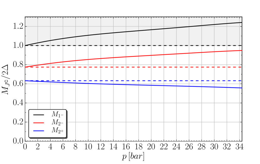
Figure 2: Strong-coupling corrections to the Bosonic masses obtained from the TDGL theory for the GL $\beta$ parameters shown in Fig. 1. The dashed lines correspond to the weak-coupling values for the masses.

In addition to the NG mode associated with broken ${\tt U(1)}_{\mbox{\footnotesize\negthickspace}}$ symmetry, there are 3 NG modes associated with spontaneously broken relative spin-orbit rotation symmetry, ${\tt SO(3)_{\text{S}}}\times{\tt SO(3)_{\text{L}}}\rightarrow{\tt SO(3)}_{\mbox{\footnotesize J}}$. These NG modes reflect the degeneracy of the BW ground state with respect to relative spin-orbit rotations, ${\tt SO(3)}_{\mbox{\footnotesize L-S}}$, whose generators form a vector representation of ${\tt SO(3)}_{\mbox{\footnotesize\negthinspace}}$. Thus, the corresponding NG modes are the $J^{\mbox{\small c}}=1^{+}$ modes, which are spin-orbit waves with excitation energies, $\omega_{1,m}=c_{1,m}|{\bf q}|$, and velocities, $c_{1,0}=\genfrac{}{}{}{1}{1}{5}v_{f}$ and $c_{1,\pm 1}=\genfrac{}{}{}{1}{2}{5}v_{f}$ in the weak-coupling limit.Popov (1987) The velocities are also renormalized in the limit $T\rightarrow 0$ by the coupling to dynamical fluctuations of the underlying Fermionic vacuum.

The partners to these NG modes are the $J^{\mbox{\small c}}=1^{-}$ Higgs modes with mass

$$M_{1,-}=2\Delta\left(\frac{-\beta_{1}+\genfrac{}{}{}{1}{1}{3}(\beta_{4}-\beta_{35})}{\beta_{12}+\genfrac{}{}{}{1}{1}{3}\beta_{345}}\right)^{\genfrac{}{}{}{1}{1}{2}}\,,$$ (19)

which reduces to $M^{\text{wc}}_{1,-}=2\Delta$ in the weak-coupling limit for the GL $\beta$ parameters (Eqs. 6). However, in the strong-coupling limit the masses of the $J^{\mbox{\small c}}=1^{-}$ modes deviate from $2m_{\text{F}}$, which implies a violation of the NSR for the $J=1$ Bosonic modes. Theoretical calculations of the strong-coupling $\beta$ parameters predict that the $J^{\mbox{\small c}}=1^{-}$ Higgs modes are pushed to energies above the pair-breaking edge of $2\Delta$, as shown in Fig. 2. This opens the possibility for the $J^{\mbox{\small c}}=1^{-}$ modes to decay into un-bound Fermion pairs. Thus, we expect the $J^{\mbox{\small c}}=1^{-}$ modes are at best resonances with finite lifetime.

For $J=2$ there are two 5-fold multiplets of Higgs modes with masses

$$M_{2,+}=2\Delta\left(\frac{\genfrac{}{}{}{1}{1}{3}\beta_{345}}{\beta_{12}+\genfrac{}{}{}{1}{1}{3}\beta_{345}}\right)^{\genfrac{}{}{}{1}{1}{2}}\,,$$ (20)

$$M_{2,-}=2\Delta\left(\frac{-\beta_{1}}{\beta_{12}+\genfrac{}{}{}{1}{1}{3}\beta_{345}}\right)^{\genfrac{}{}{}{1}{1}{2}}\,.$$ (21)

Equation 21 provides a fifth observable that might be used to determine GL $\beta$ parameters from independent experiments in the GL regime.Choi et al. (2007) In the weak-coupling limit with $\beta_{i}$ given by Eqs. 6, the masses reduce to $M_{2,+}^{\text{wc}}=\sqrt{\frac{8}{5}}\Delta$ and $M_{2,-}^{\text{wc}}=\sqrt{\frac{12}{5}}\Delta$. Thus, the $J^{\mbox{\small c}}=2^{\pm}$ Higgs modes obey the NSR in the weak-coupling limit of the TDGL theory.Nambu (1985); Volovik and Zubkov (2013, 2014)

However, the NSR is violated by strong-coupling corrections to the Higgs masses, shown in Fig. 2 as a function of pressure for the strong-coupling $\beta$ parameters shown in Fig. 1. The asymmetry in the mass corrections for $M_{2,\pm}$ leads to a sizable violation of the NSR at high pressures: $\sum_{\mbox{\small c}}M_{2,\mbox{\small c}}^{2}/4m_{\text{F}}^{2}-1\approx 20\,\%$ at $p=34\,\mbox{bar}$. The violations of the NSR have the following origin: The strong-coupling Lagrangian for the Bosonic fluctuations, Eqs. 11 and 114-118, depends on the symmetry of the mode; thus, the strong-coupling renormalization of the Higgs masses depends on $J^{\mbox{\small c}}$. For the $J=0^{+}$ mode the strong-coupling renormalization of the mass is the same as that of the $J=0^{+}$ ground state amplitude $\Delta$, and thus the Fermion mass, in which case the NSR is satisfied even with strong-coupling corrections. However, for modes with $J\neq 0$, the renormalization of the mass of the Higgs mode is a different combination of the strong-coupling $\beta$’s than that which renormalizes $\Delta$, leading to violations of the NSR.

V Beyond TDGL Theory

The TDGL theory is limited in its applicability because it is based on an effective action with only Bosonic degrees of freedom. However, the parent state of a BCS condensate is the Fermi liquid ground state (“Fermionic vacuum”). In order to calculate effects on the Bosonic spectrum arising from “back-action” of the Fermionic vacuum we require a dynamical theory that includes both Fermion and Bosonic degrees of freedom.

Microscopic formulations of the theory of collective excitations in superfluid ³He-B were developed on the basis of mean-field kinetic equations in Ref. Wölfle, 1974, Kubo theory in Refs. Maki, 1974 and Tewordt and Schopohl, 1979, a functional integral formulation of the hydrodynamic action in Ref. Brusov and Popov, 1980, and quasi-classical transport theory in Refs. Sauls and Serene, 1981b; Moores and Sauls, 1993; McKenzie and Sauls, ; McKenzie and Sauls, 2013. We highlight the coupling between Bosonic and Fermionic degrees of freedom that lead to mass shifts of the Higgs modes. Results for the mass shifts of the $J^{\mbox{\small c}}=2^{\pm}$ Higgs modes reported in Ref. Sauls and Serene, 1981b are interpreted here in terms of interactions that result from polarization of the Fermionic vacuum by the creation of a Bosonic mode that has different symmetry than that of the un-polarized vacuum. The Higgs modes with different parities, $\mbox{\small c}=\pm 1$, also polarize the Fermionic vacuum in different channels, activating different interactions and leading to different mass shifts. Thus, the violation of the $J=2$ NSR is directly related to the vacuum polarization mass shifts for the two charge conjugation partners of the $J=2$ multiplet.

V.1 Particle-Hole Self Energy

For an interacting Fermi system the two-body interaction between isolated ³He atoms is renormalized to effective interactions between low-energy Fermionic quasiparticles that are well defined excitations within a low energy band near the Fermi surface, $|\varepsilon|\leq\hbar\Omega_{c}\ll E_{f}$, and thus a shell in momentum space, $\delta p\leq\hbar\Omega_{c}/v_{f}$.

A disturbance of the vacuum state from that of an isotropic Fermi sea, e.g. by a perturbation that couples to the quasiparticle states in the vicinity of the Fermi surface, generates a polarization of the Fermionic vacuum, and a corresponding self energy correction to the energy of a Fermionic quasiparticle. The leading order correction is given by the combined external field, $u_{\alpha\beta}(p)$, plus mean-field (one loop) interaction energy associated with a particle-hole excitation of the Fermionic vacuum state,

$$\Sigma_{\alpha\beta}(p) = \quad\parbox{62.59605pt}{ \begin{picture}(18.0,18.0)\immediate\ignorespaces\immediate\ignorespaces\immediate\ignorespaces\immediate\ignorespaces\immediate\ignorespaces\put(0.0,0.0){\includegraphics{fmf_Sigma.1}}\ignorespaces\immediate\ignorespaces\immediate\ignorespaces\immediate\ignorespaces\immediate\ignorespaces\immediate\ignorespaces\immediate\ignorespaces\immediate\ignorespaces\immediate\ignorespaces\immediate\ignorespaces\immediate\ignorespaces\immediate\ignorespaces\immediate\ignorespaces\immediate\ignorespaces\immediate\ignorespaces \immediate\ignorespaces{\put(0.90005,9.0){\makebox(0.0,0.0)[r]{\footnotesize$p\;\alpha$}}\put(17.09995,9.0){\makebox(0.0,0.0)[l]{\footnotesize$p\;\beta$}}\put(9.0,18.30865){\makebox(0.0,0.0)[b]{$\hskip 1.42262pt\vspace*{-2.75mm}\large\times$}}\put(11.10876,9.0){\makebox(0.0,0.0)[l]{$\vspace*{-1.0mm}u$}}}\end{picture} }\hskip 2.84526pt+\hskip 14.22636pt\parbox{62.59605pt}{ \begin{picture}(18.0,18.0)\immediate\ignorespaces\immediate\ignorespaces\immediate\ignorespaces\immediate\ignorespaces\immediate\ignorespaces\put(0.0,0.0){\includegraphics{fmf_Sigma.2}}\ignorespaces\immediate\ignorespaces\immediate\ignorespaces\immediate\ignorespaces\immediate\ignorespaces\immediate\ignorespaces\immediate\ignorespaces\immediate\ignorespaces\immediate\ignorespaces\immediate\ignorespaces\immediate\ignorespaces\immediate\ignorespaces\immediate\ignorespaces\immediate\ignorespaces\immediate\ignorespaces\immediate\ignorespaces\immediate\ignorespaces \immediate\ignorespaces{\put(0.90005,9.0){\makebox(0.0,0.0)[r]{\footnotesize$p\;\alpha$}}\put(17.09995,9.0){\makebox(0.0,0.0)[l]{\footnotesize$p\;\beta$}}\put(9.86337,13.31784){\makebox(0.0,0.0)[b]{$\vspace*{-3.5mm}\Gamma^{\mbox{\tiny ph}}$}}}\end{picture} }\,.$$ (22)

The interaction between Fermionic quasiparticles shown in Eq. 22 is represented by a four-point vertex that sums bare two-body interactions to all orders involving all possible intermediate states of high-energy Fermions. The vertex that determines the leading order quasiparticle self energy, $\Gamma^{\text{ph}}$, defines the forward-scattering amplitude for particle and hole pairs (Landau channel) scattering within the low-energy shell near the Fermi surface.

$$\Gamma^{\mbox{\footnotesize ph}}_{\alpha\beta;\gamma\rho}(p,p^{\prime}) = p^{{}^{\prime}}\gamma p\;\alpha p^{{}^{\prime}}\rho p\;\beta \Gamma^{\mbox{\tiny ph}}$$

$$= \Gamma^{(s)}(p,p^{\prime})\delta_{\alpha\gamma}\delta_{\beta\rho}+\Gamma^{(a)}(p,p^{\prime})\vec{\sigma}_{\alpha\gamma}\cdot\vec{\sigma}_{\beta\rho}\,,$$

with amplitudes $\Gamma^{(s)}(p,p^{\prime})$ for spin-independent scattering, $\Gamma^{(a)}(p,p^{\prime})$, representing the spin-dependent “exchange” scattering amplitude. The Fermion propagator in the presence of the external perturbation, $u_{\alpha\beta}(p)$, is represented by

$$G_{\alpha\beta}(p)=\,\,\langle\psi_{\alpha}(p)\bar{\psi}_{\beta}(p)\rangle\equiv\,\,\parbox{71.13188pt}{ \begin{picture}(25.0,5.0)\immediate\ignorespaces\immediate\ignorespaces\immediate\ignorespaces\immediate\ignorespaces\immediate\ignorespaces\put(0.0,0.0){\includegraphics{fmf_G.1}}\ignorespaces\immediate\ignorespaces\immediate\ignorespaces\immediate\ignorespaces\immediate\ignorespaces\immediate\ignorespaces\immediate\ignorespaces\immediate\ignorespaces\immediate\ignorespaces\immediate\ignorespaces\immediate\ignorespaces\immediate\ignorespaces\immediate\ignorespaces \immediate\ignorespaces{\put(1.22528,2.5){\makebox(0.0,0.0)[r]{\footnotesize$\alpha$}}\put(23.77472,2.5){\makebox(0.0,0.0)[l]{\footnotesize$\beta$}}\put(2.50015,3.77487){\makebox(0.0,0.0)[b]{\footnotesize${+p}$}}\put(22.49985,3.77487){\makebox(0.0,0.0)[b]{\footnotesize${+p}$}}}\end{picture} }\quad,$$ (24)

where $p=({\bf p},\varepsilon_{n})$ is the four-momentum, $\varepsilon_{n}=(2n+1)\pi T$ is the Fermion Matsubara energy, and $\alpha$ and $\beta$ are the initial and final state spin projections defining the Fermion propagator.

For ³He quasiparticles and pairs confined to a low-energy band near the Fermi surface, the vertex function, which varies slowly with $|{\bf p}|$ in the neighborhood of the Fermi surface, can be evaluated with ${\bf p}=p_{f}\hat{p}$, $\varepsilon_{n}\rightarrow 0$ and ${\bf p}^{\prime}=p_{f}\hat{p}^{\prime}$, $\varepsilon_{n}^{\prime}\rightarrow 0$ within the low-energy band, $|\varepsilon_{n}|,|\varepsilon_{n}^{\prime}|\leq\hbar\Omega_{c}$. In the same limit, we approximate the momentum space integral as $\int\frac{d^{3}{p^{\prime}}}{(2\pi)^{3}}(\ldots)\rightarrow\int\frac{d\Omega_{\hat{p}^{\prime}}}{4\pi}N(0)\int d\xi_{{\bf p}^{\prime}}(\ldots)$. The resulting vertex part reduces to functions of the relative momenta, $A^{(s,a)}(\hat{p},\hat{p}^{\prime})=2N(0)\Gamma^{(s,a)}(p_{f}\hat{p},\varepsilon=0;p_{f}\hat{p}^{\prime},\varepsilon^{\prime}=0)$, where $N(0)$ is the density of states at the Fermi level and $\xi_{{\bf p}}=v_{f}(|{\bf p}|-p_{f})$ is the quasi-particle excitation energy in the low-energy band near the Fermi surface. Rotational invariance implies that the vertex part can be expanded in terms of basis functions of the irreducible representations of ${\tt SO(3)_{\text{L}}}$, i.e. spherical harmonics, $\{Y_{\ell,m}(\hat{p})|\,m=-\ell\ldots+\ell\}$, defined on the Fermi surface,

$$A^{(s,a)}(\hat{p},\hat{p}^{\prime})=\sum_{\ell}\,A^{(s,a)}_{\ell}\sum_{m=-\ell}^{+\ell}\,Y_{\ell,m}(\hat{p})\,Y_{\ell,m}^{*}(\hat{p}^{\prime})\,,$$ (25)

where the sum is over relative angular momentum channels, $\ell\geq 0$. The resulting spin independent ($\Sigma(\hat{p})$) and exchange ($\vec{\Sigma}(\hat{p})$) self-energies defined on the low-energy bandwidth of the interaction are given by

$$\Sigma(\hat{p}) = \Sigma_{\text{ext}}(\hat{p})+\int\,\frac{d\Omega_{\hat{p}^{\prime}}}{4\pi}\,A^{(s)}(\hat{p},\hat{p}^{\prime})\,T\sum_{\varepsilon_{n^{\prime}}}\,\negthickspace{{}^{\prime}}\,\,g(\hat{p}^{\prime},\varepsilon_{n}^{\prime})\,,$$ (26)

$$\vec{\Sigma}(\hat{p}) = \vec{\Sigma}_{\text{ext}}(\hat{p})+\int\,\frac{d\Omega_{\hat{p}^{\prime}}}{4\pi}\,A^{(a)}(\hat{p},\hat{p}^{\prime})\,T\sum_{\varepsilon_{n^{\prime}}}\,\negthickspace{{}^{\prime}}\,\vec{g}(\hat{p}^{\prime},\varepsilon_{n}^{\prime})\,,$$ (27)

where $g$ and $\vec{g}$ are the scalar and spin-vector components of the quasi-classical propagator obtained by integration over the momentum shell $-\Omega_{c}\leq v_{f}\delta p\leq\Omega_{c}$ near the Fermi surface, $\int\,d\xi_{{\bf p}}\,G_{\alpha\beta}(p)$ $\equiv$ $g_{\alpha\beta}(\hat{p},\varepsilon_{n})$ $=$ $g(\hat{p},\varepsilon_{n})\,\delta_{\alpha\beta}$ $+$ $\vec{g}(\hat{p},\varepsilon_{n})\cdot\,\vec{\sigma}_{\alpha\beta}$. Note that the Matsubara sum, $\sum\,\negthickspace{{}^{\prime}}$, is restricted to $|\varepsilon_{n}^{\prime}|\leq\hbar\Omega_{c}$, and the self energies vanish for the undisturbed Fermi sea.

V.2 Particle-Particle Self Energy

The Cooper instability results from repeated scattering of Fermion pairs with zero total momentum (Cooper channel) that leads to the formation of bound Fermion pairs. Unbounded growth of the particle-particle amplitude is regulated by the formation of a new ground state, defined in terms of a macroscopic amplitude

$$F_{\alpha\beta}(p)=\,\,\langle\psi_{\alpha}(p)\psi_{\beta}(-p)\rangle\equiv\,\,\parbox{71.13188pt}{ \begin{picture}(25.0,5.0)\immediate\ignorespaces\immediate\ignorespaces\immediate\ignorespaces\immediate\ignorespaces\immediate\ignorespaces\put(0.0,0.0){\includegraphics{fmf_F.1}}\ignorespaces\immediate\ignorespaces\immediate\ignorespaces\immediate\ignorespaces\immediate\ignorespaces\immediate\ignorespaces\immediate\ignorespaces\immediate\ignorespaces\immediate\ignorespaces\immediate\ignorespaces\immediate\ignorespaces\immediate\ignorespaces\immediate\ignorespaces \immediate\ignorespaces{\put(1.22528,2.5){\makebox(0.0,0.0)[r]{\footnotesize$\alpha$}}\put(23.77472,2.5){\makebox(0.0,0.0)[l]{\footnotesize$\beta$}}\put(2.50015,3.77487){\makebox(0.0,0.0)[b]{\footnotesize${+p}$}}\put(22.49985,3.77487){\makebox(0.0,0.0)[b]{\footnotesize${-p}$}}}\end{picture} }\quad,$$ (28)

for a condensate of Fermion pairs with zero center of mass energy and momentum. The condensate and interaction in the Cooper channel also generates an associated mean-field

$$\Delta_{\alpha\beta}(p) \,\,=\,\, +p\;\alpha -p\;\beta \vspace*{-3.5mm}\Gamma^{\mbox{\tiny pp}}$$ (29)

$$\,\,=\,\, -T\sum_{\varepsilon_{n}^{\prime}}\int\frac{d^{3}{p^{\prime}}}{(2\pi)^{3}}\,\Gamma^{\text{\footnotesize pp}}_{\alpha\beta;\gamma\rho}(p,p^{\prime})\,F_{\gamma\rho}(p^{\prime})\,,$$

where

$$\Gamma^{\mbox{\footnotesize pp}}_{\alpha\beta;\gamma\rho}(p,p^{\prime}) = +p^{{}^{\prime}}\gamma +p\;\alpha -p^{{}^{\prime}}\rho -p\;\beta \Gamma^{\mbox{\tiny pp}}$$ (30)

$$= \Gamma^{(0)}(p,p^{\prime})(i\sigma_{y})_{\alpha\beta}(i\sigma_{y})_{\gamma\rho}$$

$$+ \Gamma^{(1)}(p,p^{\prime})(i\vec{\sigma}\sigma_{y})_{\alpha\beta}\cdot(i\sigma_{y}\vec{\sigma})_{\gamma\rho}\,,$$ (31)

is the four-Fermion vertex that is irreducible in the particle-particle channel, expressed in terms of the spin-singlet ($S=0$), even-parity and spin-triplet ($S=1$), odd-parity pairing interactions, $\Gamma^{(0)}(p,p^{\prime})$ and $\Gamma^{(1)}(p,p^{\prime})$, respectively. Thus, the pairing self energy separates into singlet and triplet components

$$\Delta_{\alpha\beta}(p)=d(p)\,(i\sigma_{y})_{\alpha\beta}+\vec{d}(p)\cdot(i\vec{\sigma}\sigma_{y})_{\alpha\beta}\,.$$ (32)

Fermion pairs with binding energy $|\Delta|<\Omega_{c}$ are confined to a low-energy band near the Fermi surface, $|\varepsilon|\leq\hbar\Omega_{c}\ll E_{f}$, and a shell in momentum space, $\delta p\leq\hbar\Omega_{c}/v_{f}$. Thus, the particle-particle irreducible vertex, which varies slowly on with $|{\bf p}|$ in the neighborhood of the Fermi surface, can also be evaluated with ${\bf p}=p_{f}\hat{p}$, $\varepsilon_{n}\rightarrow 0$ and ${\bf p}^{\prime}=p_{f}\hat{p}^{\prime}$, $\varepsilon_{n}^{\prime}\rightarrow 0$. Thus, $\Gamma^{pp}$ reduces to even- and odd-parity functions of the relative momenta, $V^{(S)}(\hat{p},\hat{p}^{\prime})=2N(0)\Gamma^{(S)}(p_{f}\hat{p},\varepsilon=0;p_{f}\hat{p}^{\prime},\varepsilon^{\prime}=0)$, and rotational invariance of the normal-state Fermionic vacuum implies

$$V^{{\binom{0}{1}}}(\hat{p},\hat{p}^{\prime}) = -\sum^{\binom{\text{even}}{\text{odd}}}_{\ell}\,v_{\ell}\sum_{m=-\ell}^{+\ell}\,Y_{\ell,m}(\hat{p})\,Y_{\ell,m}^{*}(\hat{p}^{\prime})$$ (33)

$$= -\sum^{\binom{\text{even}}{\text{odd}}}_{\ell}\,(2\ell+1)\,v_{\ell}\,P_{\ell}(\hat{p}\cdot\hat{p}^{\prime})\,,$$

where the sum is over all even (odd) orbital angular momentum channels, $\ell\geq 0$, for spin-singlet (spin-triplet) pair scattering, and $-v_{\ell}$ is the pairing interaction (“coupling constant”) in the orbital angular momentum channel $\ell$. The singlet ($d(\hat{p})$) and triplet ($\vec{d}(\hat{p})$) self-energies are given by

$$d(\hat{p}) = -\int\,\frac{d\Omega_{\hat{p}^{\prime}}}{4\pi}\,V^{(0)}(\hat{p},\hat{p}^{\prime})\,\,T\sum_{\varepsilon_{n^{\prime}}}\,\negthickspace{{}^{\prime}}\,f(\hat{p}^{\prime},\varepsilon_{n}^{\prime})\,,$$ (34)

$$\vec{d}(\hat{p}) = -\int\,\frac{d\Omega_{\hat{p}^{\prime}}}{4\pi}\,V^{(1)}(\hat{p},\hat{p}^{\prime})\,\,T\sum_{\varepsilon_{n^{\prime}}}\,\negthickspace{{}^{\prime}}\,\vec{f}(\hat{p}^{\prime},\varepsilon_{n}^{\prime})\,,$$ (35)

where $f_{\alpha\beta}(\hat{p},\varepsilon_{n})$ $\equiv$ $\int\,d\xi_{{\bf p}}\,F_{\alpha\beta}(p)$ $=$ $f(\hat{p},\varepsilon_{n})\,(i\sigma_{y})_{\alpha\beta}$ $+$ $\vec{f}(\hat{p},\varepsilon_{n})\cdot\,(i\vec{\sigma}\sigma_{y})_{\alpha\beta}$ is the quasi-classical pair propagator expressed in terms of the anomalous singlet and triplet components, $f$ and $\vec{f}$.

The breaking of ${\tt U(1)}_{\mbox{\footnotesize\negthinspace}}$ symmetry by pair condensation implies mixing of normal-state particle- and hole states. Particle-hole coherence is accommodated by introducing Nambu spinors, $\Psi=\left(\psi_{\uparrow}\,,\,\psi_{\downarrow}\,,\,\psi^{{\dagger}}_{\uparrow}\,,\,\psi^{{\dagger}}_{\downarrow}\right)$, or equivalently by a $4\times 4$ Nambu matrix propagator in the combined particle-hole and spin space. In the quasi-classical limit the Nambu propagator is represented by the diagonal and off-diagonal quasiclassical propagators, $\hat{g}$ and $\hat{f}$, and their conjugates, $\hat{g}^{\prime}$ and $\hat{f}^{\prime}$,

$$\widehat{g}=\begin{pmatrix}g+\vec{g}\cdot\vec{\mbox{\boldmath$\sigma$}}&f\,i\sigma_{y}+\vec{f}\cdot i\vec{\mbox{\boldmath$\sigma$}}\sigma_{y}\\ f^{\prime}\,i\sigma_{y}+\vec{f^{\prime}}\cdot i\sigma_{y}\vec{\mbox{\boldmath$\sigma$}}&g^{\prime}-\vec{g^{\prime}}\cdot\sigma_{y}\vec{\mbox{\boldmath$\sigma$}}\sigma_{y}\end{pmatrix}\,,$$ (36)

where $g$ ($\vec{g}$) is the spin scalar (vector) component of the Fermion propagator, while $f$ ($\vec{f}$) is the spin singlet (triplet) component of the anomalous pair propagator. The lower row of the Nambu matrix represents the conjugate propagators, $\hat{\bar{g}}$ and $\hat{\bar{f}}$, which are related to $\hat{g}$ and $\hat{f}$ by the combination of Fermion anti-symmetry and particle-hole conjugation symmetries (c.f. App. X.2). Similarly, the quasiparticle and pairing self-energies are organized into a $4\times 4$ Nambu matrix,

$$\widehat{\Sigma}=\begin{pmatrix}\Sigma+\vec{\Sigma}\cdot\vec{\mbox{\boldmath$\sigma$}}&d\,i\sigma_{y}+\vec{d}\cdot i\vec{\mbox{\boldmath$\sigma$}}\sigma_{y}\\ d^{\prime}\,i\sigma_{y}+\vec{d^{\prime}}\cdot i\sigma_{y}\vec{\mbox{\boldmath$\sigma$}}&\Sigma^{\prime}-\vec{\Sigma}^{\prime}\cdot\sigma_{y}\vec{\mbox{\boldmath$\sigma$}}\sigma_{y}\end{pmatrix}\,,$$ (37)

with the corresponding symmetry relations connecting the conjugate self-energies to $\Sigma$, $\vec{\Sigma}$, $d$ and $\vec{d}$. This doubling of the Fermionic and Bosonic degrees of freedom, which is forced by the breaking of global ${\tt U(1)}_{\mbox{\footnotesize\negthinspace}}$ symmetry, is the origin of the doublets of Bosonic modes labeled by parity under charge conjugation, $\mbox{\small c}=\pm 1$, in BCS-type theories.

VI Eilenbergers’ Equations

The quasiparticle and anomalous pair propagators and self-energies, organized into $4\times 4$ Nambu matrices, obey Gorkov’s equations.Gorkov (1958) Eilenberger transformed Gorkov’s equations into a matrix transport-type equation for the quasiclassical propagator and self-energy,Eilenberger (1968)

$$\mbox{$\displaystyle\left[\,i\varepsilon_{n}{\widehat{\tau}_{3}}-\widehat{\Sigma}(\hat{p},{\bf R})\,,\,\widehat{g}\,\right]$}+i\hbar{\bf v}_{\hat{p}}\cdot\mbox{\boldmath$\nabla$}\widehat{g}=0\,.$$ (38)

In contrast to Gorkov’s equation, which is a second-order differential equation with a unit source term originating from the Fermion anti-commutation relations, Eilenberger’s equation is a homogeneous, first-order differential equation describing the evolution of the quasiclassical propagator along classical trajectories defined by the Fermi velocity, ${\bf v}_{\hat{p}}=v_{f}\hat{p}$. The form of Eilenberger’s equation in Eq. 38 governs the equilibrium propagator, including inhomogeneous states described by an external potential or a spatially varying mean pairing self-energy, $\widehat{\Delta}(\hat{p},{\bf R})$, but must be supplemented by the normalization condition,Eilenberger (1968)

$$\widehat{g}(\hat{p},\varepsilon_{n};{\bf R})^{2}=-\pi^{2}\,\widehat{1}\,,$$ (39)

which restores the constraint on the spectral weight implied by the source term in Gorkov’s equation. For the spatially homogeneous ground-state of superfluid ³He-B Eilenberger’s equation reduces to

$$\mbox{$\displaystyle\left[\,i\varepsilon_{n}{\widehat{\tau}_{3}}-\widehat{\Sigma}(\hat{p})\,,\,\widehat{g}_{0}\,\right]$}=0\,,$$ (40)

and the homogeneous self-energy, $\widehat{\Sigma}\equiv\widehat{\Delta}(\hat{p})$, is defined by the mean-field pairing self-energy for the ³He ground state,

$$\widehat{\Delta}(\hat{p})=\begin{pmatrix}0&\vec{\Delta}(\hat{p})\cdot i\vec{\sigma}\sigma_{y}\\ \vec{\Delta}(\hat{p})\cdot i\sigma_{y}\vec{\sigma}&0\end{pmatrix}\,,$$ (41)

where $\vec{\Delta}(\hat{p})=\Delta\,\hat{p}$ is the $J=0$ BW order parameter. Here and after we denote the equilibrium spin-triplet order parameter as $\vec{\Delta}$ and reserve $\vec{d}$ for the non-equilibrium fluctuations of the spin-triplet order parameter. The $4\times 4$ matrix order parameter for the BW state satisfies, $\widehat{\Delta}(\hat{p})\widehat{\Delta}(\hat{p})=-|\Delta|^{2}\,\widehat{1}$. Thus, the equilibrium propagator for the BW state is given by

$$\widehat{g}_{0}(\hat{p},\varepsilon_{n})=-\pi\frac{i\varepsilon_{n}{\widehat{\tau}_{3}}-\widehat{\Delta}(\hat{p})}{\sqrt{\varepsilon_{n}^{2}+|\Delta|^{2}}}\,.$$ (42)

Note that the diagonal component of $\widehat{g}_{0}$ is odd in frequency. This implies that the diagonal (Fermionic) self-energies, $\Sigma(\hat{p})$ and $\vec{\Sigma}(\hat{p})$ evaluated with Eq. 42, vanish in equilibrium. However, if the ground state is perturbed, e.g. by a Bosonic fluctuation of the Cooper pair condensate, the Fermionic self energy, in general, no longer vanishes.

In equilibrium, the anomalous self-energy reduces to the self-consistency equation (“gap equation”) for the spin-triplet order parameter,

$$\vec{\Delta}(\hat{p})=-\frac{\pi}{\beta}\sum_{\varepsilon_{n}}{{}^{\prime}}\int\frac{d\Omega_{\hat{p}}}{4\pi}\,V^{(1)}(\hat{p},\hat{p}^{\prime})\,\frac{\vec{\Delta}(\hat{p}^{\prime})}{\sqrt{\varepsilon_{n}^{2}+|\vec{\Delta}(\hat{p}^{\prime})|^{2}}}\,.$$ (43)

The linearized gap equation defines the instability temperatures for Cooper pairing with orbital angular momentum $\ell$,

$$\frac{1}{v_{\ell}}=\pi T_{c_{\ell}}\sum_{\varepsilon_{n}}{{}^{\prime}}\frac{1}{|\varepsilon_{n}|}\equiv K(T_{c_{\ell}})\,,$$ (44)

for attractive interactions $v_{\ell}>0$. The function $K(T)$ is a digamma function of argument, $\hbar\Omega_{c}/2\pi T\gg 1$, in which case

$$K(T)\equiv\pi T\sum_{\varepsilon_{n}}{{}^{\prime}}\,\frac{1}{|\varepsilon_{n}|}\simeq\ln\left(\frac{2e^{\gamma_{\text{E}}}}{\pi}\frac{\hbar\Omega_{c}}{T}\right)\,,$$ (45)

where $\gamma_{\text{E}}\simeq 0.57721$ is Euler’s constant. This function plays a central role in regulating the log-divergence of frequency sums in the Cooper channel. In ³He the p-wave pairing channel is the dominant attractive channel; the f-wave channel is also attractive, but sub-dominant, i.e. $0<T_{c_{3}}<T_{c_{1}}\equiv T_{c}$.

The anomalous self-energy in the p-wave channel also determines the mass (gap), $m_{\text{F}}=\Delta$, of Fermionic excitations of the Balian-Werthamer phase. In particular the p-wave projection of Eq. 43 reduces to the BCS gap equation,

$$\ln(T/T_{c})=2\pi T\sum_{n\geq 0}^{\infty}\left(\frac{1}{\sqrt{\varepsilon_{n}^{2}+\Delta^{2}}}-\frac{1}{\varepsilon_{n}}\right)\,.$$ (46)

Note that both the pairing interaction, $v_{1}$ and cutoff, $\Omega_{c}$, in Eq. 43 have been eliminated in favor of the transition temperature by regulating the log-divergent sum using Eq. 45 and the linearized gap equation for $T_{c}$, Eq. 44.

The Balian-Werthamer state, which has an isotropic gap in the Fermionic spectrum, is maximally effective in using states near the Fermi surface for pair condensation. As a result the B-phase is stable down to $T=0$ in spite of the attractive f-wave pairing interaction.Sauls (1986) Nevertheless, sub-dominant f-wave pairing plays an important role in the Bosonic excitation spectrum of the B-phase. In particular, p-wave, spin-triplet Higgs modes with $J=2$ polarize the B-phase vacuum. The $J=2$ polarization couples to f-wave, spin-triplet Cooper pair fluctuations with $J=2$, leading to mass corrections to the $J^{\mbox{\small c}}=2^{\pm}$ Higgs modes. In the following we derive the dynamical equations for the Bosonic modes including the polarization terms from the f-wave pairing channel, and self-energy corrections from the Landau channel.

VII Dynamical Equations

In order to describe the non-equilibrium response, or fluctuations relative to homogeneous equilibrium, we must generalize the low-energy quasiparticle and Cooper pair propagators to functions of two time ($\tau_{1},\tau_{2}$), or frequency ($\varepsilon_{n_{1}},\varepsilon_{n_{2}}$), variables. Specifically, we must include the dependence on the global time coordinate, $\Upsilon=(\tau_{1}+\tau_{2})/2$, or equivalently the total Matsubara energy $\omega_{m}$, in addition to the relative time difference, $\tau_{1}-\tau_{2}$, or corresponding Fermion Matsubara energy, $\varepsilon_{n}$. Thus, the $\xi_{{\bf p}}$-integrated quasiclassical propagator generalizes to $\widehat{g}(\hat{p},\varepsilon_{n})\rightarrow\widehat{g}(\hat{p},\varepsilon_{n};{\bf q},\omega_{m})$, where ${\bf q}$ is the total momentum, or wave vector for a Fourier mode associated with the center of mass coordinate, ${\bf R}$.

The space-time dynamics of the coupled system of Fermionic and Bosonic excitations of the broken symmetry ground state is encoded in the Keldysh propagator,Keldysh (1965) which is obtained here by analytic continuation to the real energy axes, e.g. $i\varepsilon_{n}\rightarrow\varepsilon+i0^{+}$ followed by $i\omega_{m}\rightarrow\omega+i0^{+}$. Thus,

$$\frac{1}{\beta}\sum_{\varepsilon_{n}}\,\widehat{g}(\varepsilon_{n};\omega_{m})\xrightarrow[i\omega_{m}\rightarrow\omega+i0^{+}]{}\int_{-\infty}^{+\infty}\,\frac{d\varepsilon}{4\pi i}\,\widehat{g}^{K}(\varepsilon;\omega)\,,$$ (47)

where $\widehat{g}^{K}(\hat{p},\varepsilon;{\bf q},\omega)$ is the real-energy, and frequency dependent Keldysh propagator. The Keldysh propagator determines the response to any space-time dependent excitation. For example the particle current is given by,

$${\bf J}=N(0)\int\frac{d\Omega_{\hat{p}}}{4\pi}\,\int\frac{d\varepsilon}{4\pi i}\,({\bf v}_{{\bf p}})\mbox{Tr}\Big{\{}{\widehat{\tau}_{3}}\widehat{g}^{K}(\hat{p},\varepsilon;{\bf q},\omega)\Big{\}}\,.$$ (48)

The off-diagonal Nambu components of the Kelysh propagator determine the Bosonic modes of the interacting Fermionic and Bosonic system. The spin-triplet Bosonic excitations are obtained from the anomalous triplet propagator, $\vec{f}^{K}$, and the self-consistent solution for the anomalous self-energy obtained by analytic continuation of Eq. 35,

$$\vec{d}(\hat{p};{\bf q},\omega)=-\int\frac{d\Omega_{\hat{p}}}{4\pi}\,V^{(1)}(\hat{p},\hat{p}^{\prime})\,\int\frac{d\varepsilon}{4\pi i}\,\vec{f}^{K}(\hat{p},\varepsilon;{\bf q},\omega)\,.$$ (49)

To calculate the Keldysh propagator, $\widehat{g}^{K}$, we generalize Eilenberger’s transport equation for the two-time/frequency non-equilibrium Matsubara propagator,

$$\left[i\varepsilon{\widehat{\tau}_{3}}-\widehat{\Sigma}\right]\circ\widehat{g}-\widehat{g}\circ\left[i\varepsilon{\widehat{\tau}_{3}}-\widehat{\Sigma}\right]+i{\bf v}_{\hat{p}}\cdot\mbox{\boldmath$\nabla$}\widehat{g}=0\,,$$ (50)

where the $A\circ B(\varepsilon_{n_{1}},\varepsilon_{n_{2}})\equiv\frac{1}{\beta}\sum_{n_{3}}\,A(\varepsilon_{n_{1}},\varepsilon_{n_{3}})\,B(\varepsilon_{n_{3}},\varepsilon_{n_{2}})$ is a convolution in Matsubara energies. For the two-frequency, non-equilibrium propagator the normalization condition is also a convolution product in Matsubara frequencies,

$$\widehat{g}\circ\widehat{g}\equiv\frac{1}{\beta}\sum_{\varepsilon_{n_{3}}}\widehat{g}(\varepsilon_{n_{1}},\varepsilon_{n_{3}})\widehat{g}(\varepsilon_{n_{3}},\varepsilon_{n_{2}})=-\pi^{2}\,\beta\delta_{\varepsilon_{n_{1}},\varepsilon_{n_{2}}}\,\widehat{1}\,.$$ (51)

If we express the full propagator as a correction to the equilibrium propagator (Eq. 42),

$$\widehat{g}(\hat{p},{\bf q};\varepsilon_{n_{1}},\varepsilon_{n_{2}})=\widehat{g}_{0}(\hat{p},\varepsilon_{n_{1}})\,\beta\delta_{\varepsilon_{n_{1}},\varepsilon_{n_{2}}}+\delta\widehat{g}(\hat{p},{\bf q};\varepsilon_{n_{1}},\varepsilon_{n_{2}})\,,$$ (52)

then to linear order in $\delta\widehat{g}$ the normalization condition for the correction to the propagator becomes after setting $\varepsilon_{n_{1}}=\varepsilon_{n}+\omega_{m}$, $\varepsilon_{n_{2}}=\varepsilon_{n}$, and $\delta\widehat{g}(\hat{p},{\bf q};\varepsilon_{n_{1}},\varepsilon_{n_{2}})\equiv\delta\widehat{g}(\hat{p},{\bf q};\varepsilon_{n},\omega_{m})$

$$\widehat{g}_{0}(\varepsilon_{n}+\omega_{m})\delta\widehat{g}(\varepsilon_{n},\omega_{m})+\delta\widehat{g}(\varepsilon_{n},\omega_{m})\widehat{g}_{0}(\varepsilon_{n})\,=\,0\,.$$ (53)

The Bosonic modes of the interacting Fermi superfluid are obtained from the linearized dynamical equations for the fluctuations of the anomalous self energy, $\delta\hat{\Delta}=\hat{\Delta}-\hat{\Delta}_{0}$, where the equilibrium self-energy, $\hat{\Delta}_{0}$, is defined by off-diagonal mean-field pairing self-energy for the ³He ground state (Eqs. 41 and 43). These fluctuations are coupled to fluctuations of the Fermionic self-energy, $\delta\hat{\Sigma}$. The coupled dynamical equations for the components of $\delta\widehat{\Sigma}(\hat{p};{\bf q},\omega)$ are obtained solving the non-equilibrium Eilenberger equation, Eq. 50, for $\widehat{g}$ to linear order in the self-energy fluctuations, $\delta\widehat{\Sigma}$. The linearized non-equilibrium Eileberger equation becomes,

$$\left\{i(\varepsilon_{n}+\omega_{m}){\widehat{\tau}_{3}}-\widehat{\Delta}(\hat{p})\right\}\,\delta\widehat{g}-\delta\widehat{g}\,\left\{i\varepsilon_{n}{\widehat{\tau}_{3}}-\widehat{\Delta}(\hat{p})\right\}-{\bf v}_{\hat{p}}\cdot{\bf q}\,\,\delta\widehat{g}$$

$$\hskip 14.22636pt+\,\widehat{g}_{0}(\hat{p},\varepsilon_{n}+\omega_{m})\,\delta\widehat{\Sigma}-\delta\widehat{\Sigma}\,\widehat{g}_{0}(\hat{p},\varepsilon_{n})=0\,.$$ (54)

The normalization conditions, Eqs. 39 and 53, combined with Eq. 42, provides a direct method of inverting Eq. 54 for the non-equilibrium quasiclassical propagator,

$$\delta\widehat{g}=\left(\frac{-1}{\pi^{2}D_{+}^{2}+({\bf v}_{\hat{p}}\cdot{\bf q})^{2}}\right)\left[D_{+}\,\left\{\widehat{g}_{0}(\varepsilon_{n}+\omega_{m})\,\delta\widehat{\Sigma}\,\widehat{g}_{0}(\varepsilon_{n})+\pi^{2}\,\delta\widehat{\Sigma}\right\}+{\bf v}_{\hat{p}}\cdot{\bf q}\,\left\{\delta\widehat{\Sigma}\,\widehat{g}_{0}(\varepsilon_{n})-\widehat{g}_{0}(\varepsilon_{n}+\omega_{m})\,\delta\widehat{\Sigma}\right\}\right]\,.$$ (55)

where $D_{+}(\varepsilon_{n},\omega_{m})=D(\varepsilon_{n}+\omega_{m})+D(\varepsilon_{n})$, and

$$D(\varepsilon_{n})\equiv\frac{-1}{\pi}\sqrt{\varepsilon_{n}^{2}+|\Delta|^{2}}\,,$$ (56)

is the denominator of the equilibrium propagator.

To calculate the mass spectrum of the Bosonic modes we need only the ${\bf q}=0$ propagators, in which case

$$\delta\widehat{g}=\frac{-1}{\pi^{2}}\frac{1}{D_{+}}\,\left\{\widehat{g}_{0}(\varepsilon_{n}+\omega_{m})\,\delta\widehat{\Sigma}\,\widehat{g}_{0}(\varepsilon_{n})+\pi^{2}\,\delta\widehat{\Sigma}\right\}\,.$$ (57)

In zero magnetic field, spin-singlet Bosonic fluctuations, if they exist, do not couple to spin-triplet Bosonic fluctuations. However, we must retain fluctuations of the Fermionic self-energy, thus the form of the fluctuation self-energy becomes,

$$\delta{\widehat{\mbox{\footnotesize$\Sigma$}}}=\begin{pmatrix}\Sigma+\vec{\Sigma}\cdot\vec{\mbox{\boldmath$\sigma$}}&\vec{d}\cdot i\vec{\mbox{\boldmath$\sigma$}}\sigma_{y}\\ \vec{d^{\prime}}\cdot i\sigma_{y}\vec{\mbox{\boldmath$\sigma$}}&\Sigma^{\prime}-\vec{\Sigma^{\prime}}\cdot\sigma_{y}\vec{\mbox{\boldmath$\sigma$}}\sigma_{y}\end{pmatrix}\,.$$ (58)

where the conjugate spin-triplet order parameter amplitudes are related by $\vec{d}^{\prime}(\hat{p};{\bf q},\omega_{m})=\vec{d}(\hat{p};-{\bf q},-\omega_{m})^{*}$ (see App. X). The linear combinations,

$$\vec{d}^{(\pm)}(\hat{p};{\bf q},\omega_{m})\equiv\vec{d}(\hat{p};{\bf q},\omega_{m})\pm\vec{d}^{\prime}(\hat{p};{\bf q},\omega_{m})\,,$$ (59)

have charge conjugation parities, $\mbox{\small c}=\pm 1$; the dynamical equations for Bosonic modes then separate into charge conjugation doublets with opposite parity. The Bosonic modes of Cooper pairs also couple to the fluctuations of the Fermionic self energy, in both the spin scalar and vector channels,

$$\Sigma^{(\pm)}(\hat{p};{\bf q},\omega_{m})\equiv\Sigma(\hat{p};{\bf q},\omega_{m})\pm\Sigma^{\prime}(\hat{p};{\bf q},\omega_{m})\,,$$ (60)

$$\vec{\Sigma}^{(\pm)}(\hat{p};{\bf q},\omega_{m})\equiv\vec{\Sigma}(\hat{p};{\bf q},\omega_{m})\pm\vec{\Sigma}^{\prime}(\hat{p};{\bf q},\omega_{m})\,.$$ (61)

Note that the exchange and conjugation symmetry relations for the diagnoal self-energies, Eqs. 123-124 and Eqs. 131-132, imply that the Fermionic self-energies, $\Sigma^{(\pm)}$ and $\vec{\Sigma}^{(\pm)}$ are also even (odd) with respect to charge conjugation parity, $\mbox{\small c}=\pm 1$.

The dynamical equations for the spin-triplet Bosonic modes are obtained from the off-diagonal and diagonal components of $\delta\widehat{g}$ in Eq. 55, the self-consistency equations for the leading order mean-field self-energies, Eqs. 26, 27 and 35. Two response functions are obtained from the propagator in Eq. 57 that determine the Bosonic and Fermionic self-energies,

$$\gamma(i\omega_{m}) = -\frac{1}{\beta}\sum_{\varepsilon_{n}}\Big{[}\frac{1}{D(\varepsilon_{n})}+\frac{1}{D(\varepsilon_{n}+\omega_{m})}\Big{]}\,,$$ (62)

$$\lambda(i\omega_{m}) = \frac{2}{\pi^{2}\beta}\sum_{\varepsilon_{n}}\frac{|\Delta^{2}|}{D_{+}(\varepsilon_{n},\omega_{m})D(\varepsilon_{n})D(\varepsilon_{n}+\omega_{m})}\,.$$ (63)

The Matsubara sum defining $\gamma(i\omega_{m})$ is log-divergent, regulated by the cutoff $\Omega_{c}$. The frequency dependence of $\gamma$ can be neglected, since it gives a negligible correction of order $(\omega_{m}/\Omega_{c})^{2}\ll 1$. Thus,

$$\frac{\mbox{\small 1}}{\mbox{\small 2}}\gamma=\frac{\pi}{\beta}\sum_{\varepsilon_{n}}{{}^{\prime}}\,\frac{1}{\sqrt{\varepsilon_{n}^{2}+|\Delta|^{2}}}=\frac{1}{v_{1}}\,,$$ (64)

where the latter equality follows from the equilibrium gap equations, Eqs. 44 - 46. The function $\lambda(i\omega_{m})$ is defined by a convergent Matsubara sum. Analytic continuation to real frequencies of Eq. 63 in the manner of Eq. 47 yields,

$$\lambda(\omega)\equiv|\Delta|^{2}\,\bar{\lambda}(\omega)=|\Delta|^{2}\int_{|\Delta|}^{\infty}\,\frac{d\varepsilon}{\sqrt{\varepsilon^{2}-|\Delta|^{2}}}\frac{\tanh\left(\frac{\beta\varepsilon}{2}\right)}{\varepsilon^{2}-\omega^{2}/4}\,,$$ (65)

which is the Tsuneto function with $\omega\rightarrow\omega+i0^{+}$ defining the retarded (causal) response.Tsuneto (1960) For $|\omega|<2|\Delta|$, $\lambda(\omega)$ is real and defines the non-resonant frequency response of the condensate, while for $|\omega|>2|\Delta|$, $\mbox{Im}\lambda(\omega)\neq 0$ is the spectral density of unbound Fermion pairs. In the $T=0$ limit, with $x=\omega/2|\Delta|$,

$$\lambda(\omega)=\left\{\begin{matrix}\displaystyle\frac{\sin^{-1}(x)}{x\sqrt{1-x^{2}}}\,\,,&|x|<1\cr&\cr\displaystyle\frac{1}{2x\sqrt{x^{2}-1}}\left[\ln\left|\frac{\sqrt{x^{2}-1}-x}{\sqrt{x^{2}-1}+x}\right|+i\pi\mbox{sgn}(x)\right]\negthinspace,&\negthinspace|x|>1\end{matrix}\right.$$ (66)

Thus, analytic continuation to real frequencies for the ${\bf q}=0$ limit leads to the following dynamical equations for the spin-triplet Bosonic modes of the B-phase ground state,Sauls and Serene (1981b); McKenzie and Sauls ; McKenzie and Sauls (2013); Moores and Sauls (1993)

$$\vec{d}^{(-)}(\hat{p};\omega) = -\int\frac{d\Omega_{p^{\prime}}}{4\pi}\,V^{(1)}(\hat{p},\hat{p}^{\prime})\,\Big{\{}\left[\frac{\mbox{\small 1}}{\mbox{\small 2}}\gamma+\frac{\mbox{\small 1}}{\mbox{\small 4}}(\omega^{2}-4|\Delta|^{2})\bar{\lambda}(\omega)\right]\,\vec{d}^{(-)}(\hat{p}^{\prime};\omega)+\bar{\lambda}(\omega)\vec{\Delta}(\hat{p}^{\prime})\,(\vec{\Delta}(\hat{p}^{\prime})\cdot\vec{d}^{(-)}(\hat{p}^{\prime};\omega))$$ (67)

$$\hskip 85.35826pt-\frac{\mbox{\small 1}}{\mbox{\small 2}}\omega\,\bar{\lambda}(\omega)\,\vec{\Delta}(\hat{p}^{\prime})\,\Sigma^{(+)}(\hat{p}^{\prime};\omega)\Big{\}}\,,$$

$$\vec{d}^{(+)}(\hat{p};\omega) = -\int\frac{d\Omega_{p^{\prime}}}{4\pi}\,V^{(1)}(\hat{p},\hat{p}^{\prime})\,\Big{\{}\left[\frac{\mbox{\small 1}}{\mbox{\small 2}}\gamma+\frac{\mbox{\small 1}}{\mbox{\small 4}}\omega^{2}\bar{\lambda}(\omega)\right]\,\vec{d}^{(+)}(\hat{p}^{\prime};\omega)-\bar{\lambda}(\omega)\vec{\Delta}(\hat{p}^{\prime})(\vec{\Delta}(\hat{p}^{\prime})\cdot\vec{d}^{(+)}(\hat{p}^{\prime};\omega))$$ (68)

$$\hskip 85.35826pt+\genfrac{}{}{}{1}{i}{2}\omega\,\bar{\lambda}(\omega)\,\vec{\Delta}(\hat{p}^{\prime})\times\vec{\Sigma}^{(+)}(\hat{p}^{\prime};\omega)\Big{\}}\,,$$

Note that the equations of motion for the Bosonic fluctuations of the order parameter couple to the Fermionic self-energies linearly in the frequency $\omega$, and that only the even orbital parity Fermionic fluctuations contribute in the ${\bf q}=0$ limit.

For the moment we omit pairing fluctuations in higher angular momentum channels, i.e. set $v_{\ell}=0$ for $\ell\geq 3$. We then expand the spin-triplet order parameter amplitudes, $\vec{d}^{(\pm)}(\hat{p})$, in terms of the p-wave basis, $d^{(\pm)}_{\alpha}(\hat{p})={\mathcal{D}}^{(\pm)}_{\alpha i}\hat{p}_{i}$, where ${\mathcal{D}}^{(\pm)}_{\alpha i}$ is equivalent to the bi-vector representation of the order parameter discussed in the context of the TDGL theory for the Bosonic modes. For the B-phase ground state with total angular momentum $J=0$, i.e. $\vec{\Delta}(\hat{p})=\Delta\hat{p}$, or equivalently, $A_{\alpha i}=\Delta/\sqrt{3}\,\delta_{\alpha i}$, Eqs. 67 and 68 can be solved by expanding the pairing fluctuations in spherical tensors that define bases for the representations of the residual symmetry group of the B-phase, $H={\tt SO(3)}_{\mbox{\footnotesize J}}$, with total angular momentum $J=0,1,2$,

$${\mathcal{D}}^{(\pm)}_{\alpha i}=\sum_{J=0,1,2}\sum_{m=-J,+J}\,D^{(\pm)}_{J,m}\,t^{(J,m)}_{\alpha i}\,.$$ (69)

Note that time-dependent fluctuations of the Fermionic self-energy, e.g. $\omega\Sigma^{(+)}(\hat{p};\omega)$, appear as “source” terms in the equations of motion for the order parameter collective modes.

VII.1 Nambu-Goldstone and Higgs Modes with $\mbox{\small c}=-1$

In the case of the modes with parity $\mbox{\small c}=-1$ we can express

$$\Sigma^{(+)}(\hat{p};\omega)=\sum_{J}^{\text{even}}\sum_{m}\,\Sigma^{(+)}_{J,m}(\omega)\,\hat{p}_{i}\,t^{(J,m)}_{ij}\,\hat{p}_{j}\,.$$ (70)

Note that only self-energy fluctuations of even $J$ couple to the Bosonic modes with $\mbox{\small c}=-1$. Equation 67 then decouples into the dynamical equations for Bosonic mode amplitudes with total angular momentum $J$. In particular, the equation for dynamical fluctuations with $J^{\mbox{\small c}}=0^{-}$ is given by

$$\omega^{2}\,D^{(-)}_{0,0}=2\,|\Delta|\,\omega\,\Sigma^{(+)}_{0,0}\,.$$ (71)

In the simplest case the $J=0$ contribution to the Fermionic self-energy represents a fluctuation in the chemical potential, i.e. $\Sigma_{0,0}^{(+)}(\omega)=2\delta\mu(\omega)$, and as discussed earlier the pairing fluctuation with $J^{\mbox{\small c}}=0^{-}$ represents time-dependent fluctuations of the phase of the B-phase ground state, i.e. $D^{(-)}_{0,0}=2i|\Delta|\,\vartheta(\omega)$. This is the massless Anderson-Bogoliubov mode, which in the time domain for ${\bf q}=0$ obeys the Josephson phase relation, $\hbar\partial_{t}\vartheta=-2\delta\mu$. As we show below this result is un-renormalized by interactions between Fermions in either particle-hole or particle-particle channels.

Projecting out the pairing fluctuations with $J^{\mbox{\small c}}=1^{-}$ from Eq. 67 yields,

$$\left(\omega^{2}-4|\Delta|^{2}\right)\,D^{(-)}_{1,m}=0\,.$$ (72)

This is a quite remarkable result: the $J^{\mbox{\small c}}=1^{-}$ pairing fluctuations do not couple to fluctuations in the Fermion self-energy. Furthermore, neither d-wave, spin-singlet, nor f-wave spin-triplet, pairing fluctuations couple the $J^{\mbox{\small c}}=1^{-}$ modes, which implies that the mass of $J^{\mbox{\small c}}=1^{-}$ Higgs modes, $M_{1,-}=2\Delta$, is un-renormalized by interactions to leading order in the expansion.

By contrast the $J^{\mbox{\small c}}=2^{-}$ modes obey the following dynamical equations

$$\Big{[}\omega^{2}-\frac{12}{5}|\Delta|^{2}\Big{]}\,D^{(-)}_{2,m}=\frac{4}{5}\,|\Delta|\,\omega\,\Sigma^{(+)}_{2,m}\,.$$ (73)

In the absence of Fermion interactions in the particle-hole channel $\Sigma^{(+)}_{2,m}(\omega)$ represents external stress fluctuations, $u^{(+)}_{2,m}(\omega)$ that couple directly to the $J^{\mbox{\small c}}=2^{-}$ Bosonic modes. In this case the mass of the this Higgs mode is equal to the weak-coupling TDGL result, $M_{2,-}=\sqrt{12/5}\,\Delta$, but now extended to all temperatures. However, the weak-coupling result for the mass of the $J^{\mbox{\small c}}=2^{-}$ Higgs mode is renormalized by Fermionic interactions. Qualitatively this is expected given that external stress fluctuations couple directly to the $J^{\mbox{\small c}}=2^{-}$ pairing fluctuations. Excitation of a $J^{\mbox{\small c}}=2^{-}$ Higgs Boson polarizes the $J=0$ Fermionic vacuum, inducing a Fermionic self-energy correction of the same symmetry that couples back to generate a mass correction to the $J^{\mbox{\small c}}=2^{-}$ Higgs modes. The polarization correction to the Higgs mass is encoded in Eq. 137 in the limit ${\bf q}=0$, which can be expressed as

$$\Sigma^{(+)}(\hat{p};\omega) = u^{(+)}(\hat{p};\omega)$$ (74)

$$+ \int\frac{d\Omega_{\hat{p}^{\prime}}}{4\pi}\,F^{s}(\hat{p},\hat{p}^{\prime})\,\Big{\{}-\lambda(\omega)\,\Sigma^{(+)}(\hat{p}^{\prime};\omega)\,$$

$$+ \genfrac{}{}{}{1}{1}{2}\bar{\lambda}(\omega)\,\omega\,\vec{\Delta}(\hat{p}^{\prime})\cdot\vec{d}^{(-)}(\hat{p}^{\prime};\omega)\Big{\}}\,,$$

where $u^{(+)}(\hat{p};\omega)$ represents un-renormalized external forces coupling to excitations of ³He-B, and we have expressed the dynamical self-energy in terms of the spin-symmetric particle-hole irreducible interaction, $F^{s}(\hat{p},\hat{p}^{\prime})$ (c.f. Appendix X.3). Projecting out the amplitudes with $J=0,2$ defined in Eq. 70 gives,

$$\left(1+F^{s}_{0}\,\lambda(\omega)\right)\Sigma^{(+)}_{0,0}(\omega) = u_{0,0}(\omega)$$

$$+ F^{s}_{0}\,\lambda(\omega)\,\left(\frac{\omega}{2|\Delta|}\right)\,D^{(-)}_{0,0}(\omega)\,,$$

$$\left(1+\genfrac{}{}{}{1}{1}{5}F^{s}_{2}\,\lambda(\omega)\right)\Sigma^{(+)}_{2,m}(\omega) = u_{2,m}(\omega)$$

$$+ \genfrac{}{}{}{1}{1}{5}F^{s}_{2}\,\lambda(\omega)\,\left(\frac{\omega}{2|\Delta|}\right)\,D^{(-)}_{2,m}(\omega)\,.$$

The key result shown in Eqs. VII.1-VII.1 is that excitation of pairing fluctuations, $D^{(-)}_{J,m}(\omega)$, polarizes the condensate and generates internal stresses that are proportional to: (i) interactions in the particle-hole channel, $F^{s}_{2,0}$, (ii) the time-derivative of the Bosonic mode amplitudes, $\omega\,D^{(-)}_{J,m}(\omega)$, and (iii) the dynamical response of the condensate, $\lambda(\omega)$, even in the absence of bulk external forces, i.e. $u_{J,m}(\omega)=0$. In the case of the $J^{\mbox{\small c}}=0^{-}$ mode, combining Eq. 71, with $\Sigma^{(+)}_{0,0}(\omega)$ now given by Eq. VII.1 still yields the unrenormalized dynamical equation for excitation of the Anderson-Bogoliubov phase mode,

$$\omega^{2}\,D^{(-)}_{0,0}=2\,|\Delta|\,\omega\,u^{(+)}_{0,0}\,.$$ (77)

The interaction, $F^{s}_{0}$, drops out because the polarization induced by the $J^{\mbox{\small c}}=0^{-}$ Bosonic mode has the same rotational symmetry as the vacuum state.

However, in the case of the $J^{\mbox{\small c}}=2^{-}$ Higgs modes, combining Eq. 73 with $\Sigma^{(+)}_{2,m}(\omega)$ given by Eq. VII.1, yields

$$D^{(-)}_{2,m}=\frac{\frac{4}{5}\,|\Delta|\,\omega\,u^{(+)}_{2,m}(\omega)}{\Big{[}\omega^{2}-\frac{12}{5}|\Delta|^{2}+\lambda(\omega)\,\genfrac{}{}{}{1}{3}{25}\,F^{s}_{2}\,\left(\omega^{2}-4|\Delta|^{2}\right)\Big{]}}\,,$$ (78)

which has a pole at $\omega=M_{2,-}$, the renormalized mass of the $J^{\mbox{\small c}}=2^{-}$ mode. Before discussing the quantitative effect of the Landau interaction on the $J^{\mbox{\small c}}=2^{-}$ Higgs mass, we consider the effect of interactions in the Cooper channel.

VII.2 F-wave interactions in the Cooper channel

Theoretical models for fermionic interactions in the particle-particle (Cooper) channel based on exchange of long-lived ferromagnetic spin-fluctuations predict p-wave spin-triplet pairing with sub-dominant attraction in the f-wave Cooper channel, including a strong sub-dominant f-wave attractive interaction at high pressures.Layzer and Fay (1974); Fay (1975) The masses of the $J^{\mbox{\small c}}=2^{-}$ modes are sensitive to fermionic interactions in the particle-particle channel, the most relevant being the f-wave, spin-triplet channel. Pairing fluctuations in the Cooper channel couple to the p-wave, spin-triplet modes with $J=2$ leading to re-normalization of the mass of the $J^{\mbox{\small c}}=2^{\pm}$ Higss modes. Note that f-wave pairing fluctuations do not couple to the $J=0,1$ Bosonic modes.

The generalization of Eqs. 73 and VII.1 to include the f-wave pairing channel in the dynamics of the $J^{\mbox{\small c}}=2^{-}$ modes is obtained from Eqs. 67 and 74 by retaining both p-wave and f-wave pairing amplitudes,

$$d_{\alpha}^{(-)}(\hat{p})={\mathcal{D}}_{\alpha i}^{(-)}\,\hat{p}_{i}+{\cal F}_{\alpha;ijk}^{(-)}\,\hat{p}_{i}\hat{p}_{j}\hat{p}_{k}\,$$ (79)

where ${\mathcal{D}}_{\alpha i}^{(-)}$ is a second-rank tensor under the residual symmetry group of the B-phase, ${\tt SO(3)}_{\mbox{\footnotesize J}}$, representing p-wave, spin-triplet fluctuations with odd charge conjugation parity (Eq. 69), and ${\cal F}_{\alpha;ijk}^{(-)}$ is a fourth-rank tensor with f-wave orbital symmetry, and thus is completely symmetric and traceless in any pair of the orbital indices ($ijk$). Spin-triplet, f-wave pairing fluctuations couple only to the $J=2$ p-wave, triplet modes. Thus, for pure $J=2$, $S=1$, $\ell=3$ fluctuations,

$${\cal F}_{\alpha;ijk}^{(-)}=\genfrac{}{}{}{1}{5}{9}\left\{\right. \left(\delta_{\alpha i}{\cal F}_{jk}^{(-)}+\delta_{\alpha j}{\cal F}_{ik}^{(-)}+\delta_{\alpha k}{\cal F}_{ij}^{(-)}\right)$$

$$-\genfrac{}{}{}{1}{2}{5} \left.\left({\cal F}_{\alpha i}^{(-)}\delta_{jk}+{\cal F}_{\alpha j}^{(-)}\delta_{ik}+{\cal F}_{\alpha k}^{(-)}\delta_{ij}\right)\right\}\,,$$ (80)

where by contraction

$${\cal F}^{(-)}_{jk}\equiv\genfrac{}{}{}{1}{3}{7}\,{\cal F}^{(-)}_{\alpha;\alpha jk}\,,$$ (81)

is a rank two, traceless and symmetric $J=2$ tensor. In particular, we can expand ${\cal F}^{(-)}_{ij}$ in the $J=2$ base tensors,

$${\cal F}^{(-)}_{ij}=\sum_{m=-2}^{+2}\,F^{(-)}_{2,m}\,t^{(2,m)}_{ij}\,.$$ (82)

The $J=2^{-}$ gap distortion is determined by both the p- and f-wave $J=2$ tensors,

$$\vec{\Delta}(\hat{p})\cdot\vec{d}^{(-)}(\hat{p};\omega)=\Delta\,\left({\mathcal{D}}^{(-)}_{ij}+{\cal F}^{(-)}_{ij}\right)\hat{p}_{i}\hat{p}_{j}\,,$$ (83)

and thus the $J=2^{-}$ component of the Fermionic self-energy induced by the $J^{\mbox{\small c}}=2^{-}$ Higgs modes (c.f. Eq. VII.1) becomes,

$$\left(1+\genfrac{}{}{}{1}{1}{5}F^{s}_{2}\,\lambda(\omega)\right)\Sigma^{(+)}_{2,m}(\omega) = u_{2,m}(\omega)+\genfrac{}{}{}{1}{1}{5}F^{s}_{2}\,\lambda(\omega)$$

$$\times \left(\frac{\omega}{2|\Delta|}\right)\left[D^{(-)}_{2,m}(\omega)+F^{(-)}_{2,m}(\omega)\right]\,.$$

The $J^{\mbox{\small c}}=2^{-}$ amplitudes satisfy coupled time-dependent gap equations obtained by projecting out the p- and f-wave components of Eq. 67 where $v_{\ell}$ are the pairing interactions in orbital angular momentum channel, $\ell=1,3,\ldots$. The p-wave interaction is the dominant attractive channel. The relevant measure of the strength of the sub-dominant f-wave pairing interaction is

$$x_{3}^{-1}\equiv\left(\frac{1}{v_{1}}-\frac{1}{v_{3}}\right)^{-1}=\ln\left(T_{c_{3}}/T_{c}\right)^{-1}\,,$$ (85)

where $x_{3}^{-1}<0$ ($x_{3}^{-1}>0$) for attractive (repulsive) f-wave pairing. The latter equality, valid for attractive f-wave pairing, is obtained from Eq. 44 for the eigenvalue spectrum of the linearized gap equation, with $T_{c}$ the p-wave transition temperature and $T_{c_{3}}$ the f-wave instability temperature for sub-dominant f-wave pairing.

Projecting out the $\ell=1$, $J=2$ component of Eq. 67, which generalizes Eq. 73, leads to

$$\Big{[}\omega^{2}-\genfrac{}{}{}{1}{12}{5}|\Delta|^{2}\Big{]}\,D^{(-)}_{2,m}+\genfrac{}{}{}{1}{8}{5}|\Delta|^{2}\,F^{(-)}_{2,m}=\genfrac{}{}{}{1}{4}{5}\,|\Delta|\,\omega\,\Sigma^{(+)}_{2,m}\,.$$ (86)

Projecting out the $\ell=3$ amplitudes from Eq. 67 gives

$$\Big{[}x_{3}+\genfrac{}{}{}{1}{1}{4}\bar{\lambda}(\omega)(\omega^{2}-4|\Delta|^{2})\Big{]}\,d^{(3,-)}_{\alpha}(\hat{p};\omega)\hskip 56.9055pt$$ (87)

$$+7\int\frac{d\Omega_{\hat{p}^{\prime}}}{4\pi}\,P_{3}(\hat{p}\cdot\hat{p}^{\prime})\,\left\{\bar{\lambda}(\omega)\,\Delta_{\alpha}(\hat{p}^{\prime})\,\vec{\Delta}(\hat{p}^{\prime})\cdot\vec{d}^{(-)}(\hat{p}^{\prime};\omega)\right.$$

$$\left.=\genfrac{}{}{}{1}{1}{2}\bar{\lambda}(\omega)\,\omega\,\Delta_{\alpha}(\hat{p}^{\prime})\,\Sigma^{+}(\hat{p}^{\prime};\omega)\right\} \,.$$

The $J=2$ components of Eq. 87 are obtained by contracting with $\hat{p}_{\alpha}$ to obtain an equation for $F^{(-)}(\hat{p})\equiv{\cal F}^{(-)}_{ij}\hat{p}_{i}\hat{p}_{j}$, then evaluating the angular average using the addition theorem for the Legendre polynomials, $(\hat{p}\cdot\hat{p}^{\prime})\,P_{3}(\hat{p}\cdot\hat{p}^{\prime})=\genfrac{}{}{}{1}{1}{7}\left\{4\,P_{4}(\hat{p}\cdot\hat{p}^{\prime})+3\,P_{2}(\hat{p}\cdot\hat{p}^{\prime})\right\}$, to obtain

$$\Big{[}\bar{x}_{3}+\genfrac{}{}{}{1}{1}{4}(\omega^{2}-\genfrac{}{}{}{1}{8}{5}|\Delta|^{2})\Big{]}F_{2,m}^{(-)}+\genfrac{}{}{}{1}{3}{5}|\Delta|^{2}\,D^{(-)}_{2,m}=\genfrac{}{}{}{1}{3}{10}\,|\Delta|\,\omega\,\Sigma_{2,m}^{+}\,,$$ (88)

where $\bar{x}_{3}\equiv x_{3}/\bar{\lambda}(\omega)$. Eliminating the Fermionic self-energy between Eqs. 86 and 88 gives the sub-dominant f-wave, $J^{\mbox{\small c}}=2^{-}$ amplitude in terms of the dominant p-wave, $J^{\mbox{\small c}}=2^{-}$,

$$\Big{[}\bar{x}_{3}+\genfrac{}{}{}{1}{1}{4}(\omega^{2}-4|\Delta|^{2})\Big{]}F_{2,m}^{(-)}=\genfrac{}{}{}{1}{3}{8}(\omega^{2}-4|\Delta|^{2})\,D^{(-)}_{2,m}\,.$$ (89)

The total $J^{\mbox{\small c}}=2^{-}$ Higgs amplitude - the sum of the p- and f-wave amplitudes, $H^{(-)}_{2,m}(\omega)\equiv D^{(-)}_{2,m}+F^{(-)}_{2,m}$ - that polarizes the Fermionic vacuum (Eq. VII.1) is governed by the dynamical equation obtained by combining Eqs. 86 and 89. This gives the retarded propagator for the $J^{\mbox{\small c}}=2^{-}$ Higgs mode,

$$H^{(-)}_{2,m}=\frac{\frac{4}{5}\,|\Delta|\,\omega\,u^{(+)}_{2,m}(\omega)\,\left[1+\genfrac{}{}{}{1}{5}{8}\,x_{3}^{-1}\,(\omega^{2}-4|\Delta|^{2})\bar{\lambda}(\omega)\right]}{\Big{[}\omega^{2}-\frac{12}{5}|\Delta|^{2}+\lambda(\omega)\,(\omega^{2}-4|\Delta|^{2})\,\left(\genfrac{}{}{}{1}{3}{25}\,F^{s}_{2}\,+({\omega}/{2|\Delta|})^{2}\,x_{3}^{-1}\right)\Big{]}}\,.$$ (90)

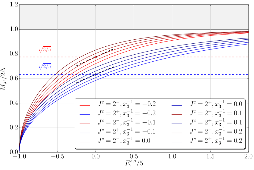
Figure 3: Masses of the $J^{\mbox{\small c}}=2^{\pm}$ Higgs modes vs. $\ell=2$ particle-hole ($F_{2}^{s,a}$) and f-wave pairing ($x_{3}^{-1}$) interactions at $T=0$. The perturbative results (Eqs. 92 and 113) for $x_{3}^{-1}=0$ are shown as the dashed black lines.

The renormalized $J^{\mbox{\small c}}=2^{-}$ Higgs mass is obtained from the pole of the propagator in Eq. 90. In the limit $T\rightarrow T_{c}^{-}$ the Tsuneto function scales as $\lambda(\omega=M_{2,-})\propto\Delta(T)/T_{c}\rightarrow 0$. Thus, the $J^{\mbox{\small c}}=2^{-}$ Higgs mass scales to the the weak-coupling TDGL result at $T_{c}$,

$$M_{2^{-}}\approx\sqrt{\frac{12}{5}}\Delta(T)\,\Bigg{[}1+\frac{\pi}{10}\sqrt{\frac{5}{2}}\,\frac{\Delta(T)}{T_{c}}\,(F^{s}_{2}/5+x_{3}^{-1})\Bigg{]}\,,$$ (91)

However, the leading order correction to the mass, $\propto\Delta(T)/T_{c}\sim(1-T/T_{c})^{\genfrac{}{}{}{1}{1}{2}}$, onsets rapidly below $T_{c}$. Thus, mass renormalzation becomes significant, of order $F_{2}^{2}$ or $x_{3}^{-1}$, for $T\rightarrow 0$. For weak interactions in both the Landau and Cooper channels, $|F_{2}^{s}|\ll 1$ and $|x_{3}^{-1}|\ll 1$, at $T=0$ the renormalized mass obtained from the pole of the $J^{\mbox{\small c}}=2^{-}$ propagator in Eq. 90 is

$$M_{2^{-}}\approx\sqrt{\frac{12}{5}}\Delta\,\Bigg{[}1+a\,(F^{s}_{2}/5+x_{3}^{-1})\Bigg{]}\,,$$ (92)

where $a=\genfrac{}{}{}{1}{1}{\sqrt{6}}\arcsin\left(\sqrt{\genfrac{}{}{}{1}{3}{5}}\right)\approx 0.362$. The Landau channel interaction $F_{2}^{s}$ obtained from measurements of the zero sound velocity ranges from $F_{2}^{s}\approx 0.5$ at $P=0\,\mbox{bar}$ to $F_{2}^{s}\approx 1.0$ at $P=34\,\mbox{bar}$, although earlier measurements reported $F_{2}^{s}\approx-0.5$ at $p=0\,\mbox{bar}$.Haard (2000)

The f-wave interaction in the Cooper has been determined from measurements of the mass of the $J^{\mbox{\small c}}=2^{-}$, $m=0$ Higgs mode based on resonant absorption of longitudinal zero sound. These experiments yield results ranging from $x_{3}^{-1}\approx 0.0$ at $p=0\,\mbox{bar}$ to $x_{3}^{-1}\approx-0.5$ at $p=14\,\mbox{bar}$ (c.f. Fig. 50 in Ref. Halperin and Varoquaux, 1990). Determinations of the mass of the $J^{\mbox{\small c}}=2^{-}$, $m=\pm 1$ Higgs modes based on transverse sound propagation and acoustic Faraday rotation by Lee et al.Lee et al. (1999); Sauls (2000), as well as more recent measurements by Collett et al.Collett et al. (2013) yield attractive f-wave interactions of similar magnitude. The f-wave interaction in the Cooper channel also contributes to the nonlinear nuclear magnetic susceptibility for the B-phase.Fishman and Sauls (1986) Analysis of magnetic susceptibility measurements of Hoyt et al.Hoyt et al. (1981) yields a stronger, but sub-dominant, attractive f-wave interaction with $x_{3}^{-1}\simeq-1.75$ ($T_{c_{3}}/T_{c}\simeq 0.56$) at low pressure.Fishman and Sauls (1988b)

Figure 3 shows the mass of the $J=2^{\mbox{\small c}}=2^{-}$ Higgs mode as a function of $F^{s}_{2}$ for various values of the f-wave pairing interaction, $x_{3}^{-1}$, obtained from numerical solution for the pole of the propagator, $H^{(-)}_{2,m}$, in Eq. 90. Note that ‘repulsive’ interactions in either channel ($F_{2}^{s,a}>0$ or $x_{3}^{-1}>0$) push the mass above the weak-coupling result towards the mass of un-bound Fermion pairs, while ’attractive interactions’ soften the mode. In particular, $M_{2,-}\rightarrow 0$ for $F_{2}^{s}/5\rightarrow-1$, signaling a dynamical instability of the ground-state. The soft mode is the dynamical signature of the Pomeranchuk instability of the underlying Fermionic vacuum.Baym and Pethick (1991)

VII.3 Nambu-Goldstone and Higgs Modes with $\mbox{\small c}=+1$

In the case of the Bosonic modes with parity $\mbox{\small c}=+1$ the Fermion self-energy that couples to these modes is expressed in terms of the momentum-dependent exchange field, $\vec{\Sigma}^{(+)}(\hat{p};\omega)$. Equation 68 decouples into the dynamical equations for Bosonic mode amplitudes with total angular momentum $J$, with orbital angular momentum $\ell=1$, $D^{(+)}_{J,m}$, and $\ell=3$, $F^{(+)}_{J,m}$. The self-energy fluctuations originating from the exchange contribution to the quasiparticle interaction are even under $\hat{p}\rightarrow-\hat{p}$; thus only fluctuations with even $J$ couple to the Bosonic modes for $\mbox{\small c}=+1$. To obtain the dynamical equations for the $J^{+}$ modes it is convenient to introduce

$$\vec{G}^{(+)}(\hat{p};\omega)=\vec{\Delta}(\hat{p})\times\vec{\Sigma}^{(+)}(\hat{p};\omega)/|\vec{\Delta}(\hat{p})|\,,$$ (93)

For the $J=0^{+}$ ground state $\vec{G}^{(+)}(\hat{p};\omega)=\hat{p}\times\vec{\Sigma}^{(+)}$ is a vector under spin rotations, odd under $\hat{p}\rightarrow-\hat{p}$ and enters Eq. 68 acts as an effective source field for Cooper pair fluctuations with $\mbox{\small c}=+1$.

It is sufficient to retain only the $\ell=0$ and $\ell=2$ contributions to the particle-hole exchange interaction, $F^{a}(\hat{p},\hat{p}^{\prime})=F^{a}_{0}+F^{a}_{2}\,P_{2}(\hat{p}\cdot\hat{p})$, in which case we can express the vector components of the quasi-particle exchange field in terms $\ell=0$ and $\ell=2$ spherical tensors,

$$\Sigma_{\gamma}^{(+)}(\hat{p};\omega)=\Sigma_{\gamma}^{(0)}+\Sigma^{(2)}_{\gamma:ij}\,\hat{p}_{i}\hat{p}_{j}\,,$$ (94)

where $\Sigma^{(2)}_{\gamma:ij}$ is traceless and symmetric in the indices, $ij$. The vector function, $\vec{G}^{(+)}(\hat{p};\omega)$, by construction contains only p-wave and f-wave orbital components, $\vec{G}^{(+)}(\hat{p};\omega)=\vec{G}^{(1)}(\hat{p};\omega)+\vec{G}^{(3)}(\hat{p};\omega)$, with $G^{(\ell)}_{\gamma}(\hat{p})=\langle(2\ell+1)\,P_{\ell}(\hat{p}\cdot\hat{p}^{\prime})\,G^{(+)}_{\gamma}(\hat{p}^{\prime})\rangle_{\hat{p}^{\prime}}$, where $\langle\ldots\rangle_{\hat{p}}\equiv\int d\Omega_{\hat{p}}/4\pi(\ldots)$. Equivalently, the p-wave contribution is defined by a second-rank tensor under joint spin- and orbital rotations,

$$G^{(1)}_{\gamma i} = \langle 3\,\hat{p}_{i}\,G^{(+)}_{\gamma}(\hat{p})\rangle_{\hat{p}}=\varepsilon_{\alpha i\gamma}\Sigma_{\gamma}^{(0)}+\frac{2}{5}\varepsilon_{\alpha j\gamma}\Sigma^{(2)}_{\gamma:ji}$$ (95)

$$= G^{(1,0)}_{\gamma i}+G^{(1,1)}_{\gamma i}+G^{(1,2)}_{\gamma i}\,,$$ (96)

where the second equation is the reduction in terms of $J=0,1,2$ tensors. The $J=0$ component is defined by the trace, which is easily seen to vanish, i.e. $G^{(1,0)}_{\alpha i}\equiv 0$. The $J=1$ components can be expressed in terms of an axial vector,

$$G^{(1,1)}_{\alpha i}=\varepsilon_{\alpha i\nu}\,G^{(1,1)}_{\nu}\,\,\mbox{with}\,\,G^{(1,1)}_{\nu}=\Sigma^{(0)}_{\nu}-\genfrac{}{}{}{1}{1}{5}\,\Sigma^{(2)}_{\gamma:\gamma\nu}\,.$$ (97)

Finally, the $J=2$ components are determined by the traceless, symmetric tensor

$$G^{(1,2)}_{\alpha i}=\genfrac{}{}{}{1}{1}{5}\left(\varepsilon_{\alpha j\gamma}\,\Sigma^{(2)}_{\gamma:ji}+\varepsilon_{ij\gamma}\,\Sigma^{(2)}_{\gamma:j\alpha}\right)\,,$$ (98)

which can be expanded in the basis of $J=2$ tensors,

$$G^{(1,2)}_{\alpha i}=\sum_{m=-2}^{+2}\,G_{2,m}\,t^{(2,m)}_{\alpha i}\,.$$ (99)

These contributions to the exchange field couple to the Bosonic mode amplitudes with quantum numbers, $J,m$ and $\mbox{\small c}=+1$, represented by second- and fourth-rank tensors that are the $\mbox{\small c}=+1$ complements of those in Eq. 79,

$$d_{\alpha}^{(+)}(\hat{p})={\mathcal{D}}_{\alpha i}^{(+)}\,\hat{p}_{i}+{\cal F}_{\alpha;ijk}^{(+)}\,\hat{p}_{i}\hat{p}_{j}\hat{p}_{k}\,,$$ (100)

where the spin-triplet, p-wave order parameter fluctuations are expanded in the basis of tensors with $J=0,1,2$,

$${\mathcal{D}}_{\alpha i}^{(+)}=\sum_{J=0,1,2}\sum_{m=-J}^{J}\,D_{J,m}^{(+)}\,t^{(J,m)}_{\alpha i}\,,$$ (101)

and similarly for spin-triplet, f-wave fluctuations with $J=2^{+}$, ${\cal F}_{\alpha i}^{(+)}=\sum_{m=-2}^{+2}\,F_{2,m}^{(+)}\,t^{(2,m)}_{\alpha i}$ where ${\cal F}_{\alpha i}^{(+)}=\genfrac{}{}{}{1}{3}{7}{\cal F}_{\gamma:\gamma\alpha i}$

The equation governing the $J^{\mbox{\small c}}=0^{+}$ mode is

$$\left(\omega^{2}\,-4|\Delta|^{2}\right)D^{(+)}_{0,0}=0\,.$$ (102)

This is the dynamical equation for the Higgs mode with the exact quantum numbers of the B-phase vacuum state. As a result there is no coupling to the $J^{\mbox{\small c}}=0^{+}$ mode via acoustic or magnetic fluctuations.

The $J^{\mbox{\small c}}=1^{+}$ modes are Nambu-Goldstone modes associated with broken relative spin-orbit rotation symmetry. It is convenient to express these mode amplitudes in the Cartesian representation, $D^{(+,1)}_{\alpha}=\genfrac{}{}{}{1}{1}{2}\varepsilon_{\alpha\beta\gamma}\,{\mathcal{D}}^{(+)}_{\beta\gamma}$. Projecting out these amplitudes from Eq. 68 yields,

$$i\omega\,D^{(+,1)}_{\alpha}=2\Delta\,\frac{1+\genfrac{}{}{}{1}{1}{15}\lambda(\omega)\,F_{2}^{a}}{1-\genfrac{}{}{}{1}{2}{45}\lambda(\omega)^{2}\,F_{0}^{a}\,F_{2}^{a}}\,\left(-\genfrac{}{}{}{1}{\gamma\hbar}{2}\,H_{\alpha}(\omega)\right)\,,$$ (103)

where $H_{\alpha}(\omega)$ is the Fourier component of the time-dependent external magnetic field and $\gamma$ is the gyromagnetic ratio of ³He. Exchange interactions renormalize the coupling of the $J^{\mbox{\small c}}=1^{+}$ modes to an external field, but the massless NG mode is protected by the continuous degeneracy of the BW ground state with respect to relative spin-orbit rotations. At finite wavelength these excitations correspond spin waves mediated by $J^{\mbox{\small c}}=1^{+}$ NG modes of the Cooper pairs with dispersion given by $\omega=c_{m}\,q$, where $c_{m}$ are the spin-wave velocities in ³He-B. See Sec. VII.4 discussion of weak symmetry-breaking perturbations on the $J^{\mbox{\small c}}=1^{+}$ modes.

The $J^{\mbox{\small c}}=2^{+}$ excitations obey the dynamical equations,

$$\Big{[}\omega^{2}-\frac{8}{5}|\Delta|^{2}\Big{]}\,D^{(+)}_{2,m}=\frac{8}{5}|\Delta|^{2}\,F^{(+)}_{2,m}-i\omega(2\Delta)\,G_{2,m}\,.$$ (104)

In the absence of Fermion interactions in the particle-particle channel the f-wave amplitude vanishes, $F^{(+)}_{2,m}\equiv 0$. And, if we also ignore Fermionic interactions in the particle-hole channel, then $G_{2,m}(\omega)$ represents an external field that couples to directly to the $J^{\mbox{\small c}}=2^{+}$ modes. In this case the mass of this Higgs mode is equal to the weak-coupling result, $M_{2,+}=\sqrt{8/5}\,\Delta$. However, $M_{2,+}$ is renormalized by Fermionic interactions in both the particle-particle and particle-hole channels. Just as in the case for the $J^{\mbox{\small c}}=2^{-}$ modes excitation of a $J^{\mbox{\small c}}=2^{+}$ Higgs Boson polarizes the $J=0^{+}$ Fermionic vacuum and introduces a Fermionic self-energy correction with the same symmetry that couples back to generate a mass correction to the $J^{\mbox{\small c}}=2^{+}$ Higgs modes.

In addition, pairing interactions in the spin-triplet, f-wave channel lead to dynamical excitations of the B-phase vacuum with spin $J^{\mbox{\small c}}=2^{+},m$, i.e. $F^{(+)}_{2,m}$, which mixes with the spin-triplet, p-wave modes of the same symmetry. We obtain the dynamical equation for the $F^{(+)}_{2,m}$ amplitudes by projecting out the f-wave orbital components of Eq. 68 to obtain,

$$\Big{[}4\bar{x}_{3}+(\omega^{2}-\frac{12}{5}|\Delta|^{2})\Big{]}\,F^{(+)}_{2,m}+\frac{12}{5}|\Delta|^{2}\,D^{(+)}_{2,m}=+i\omega(2\Delta)\,G_{2,m}\,,$$ (105)

where $\bar{x}_{3}\equiv x_{3}/\bar{\lambda}(\omega)$. Note that we have used the identity, $\hat{p}\cdot\vec{G}(\hat{p})=\hat{p}\cdot\vec{G}^{(1)}(\hat{p})+\hat{p}\cdot\vec{G}^{(3)}(\hat{p})\equiv 0$ to express the source term in Eq. 105 in terms of the p-wave, $J=2$ component of $\vec{G}(\hat{p})$, i.e. $G^{(3,2)}_{\gamma i}=-G^{(1,2)}_{\gamma i}$. Eliminating $G_{2,m}$ from Eqs. 104 and 105 gives the f-wave, $J^{\mbox{\small c}}=2^{+}$ amplitude in terms of the corresponding dominant p-wave amplitude,

$$\Big{[}4\bar{x}_{3}+(\omega^{2}-4|\Delta|^{2})\Big{]}\,F^{(+)}_{2,m}=-(\omega^{2}-4|\Delta|^{2})\,D^{(+)}_{2,m}\,.$$ (106)

The polarization corrections to the $J^{\mbox{\small c}}=2^{+}$ Higgs mass are obtained from Eqs. 104, 106 and 139 in the limit ${\bf q}=0$, which can be expressed as

$$\vec{\Sigma}^{(+)}(\hat{p};\omega) = \vec{h}^{(+)}(\hat{p};\omega)+\int\frac{d\Omega_{\hat{p}^{\prime}}}{4\pi}\,F^{a}(\hat{p},\hat{p}^{\prime})\,\Big{\{}$$ (107)

$$- \lambda(\omega)\,\left(\vec{\Sigma}^{(+)}(\hat{p}^{\prime};\omega)\,-\hat{p}^{\prime}(\hat{p}^{\prime}\cdot\vec{\Sigma}^{(+)}(\hat{p}^{\prime};\omega))\right)$$

$$- \left(\frac{\omega}{2\Delta}\right)\lambda(\omega)\,\hat{p}^{\prime}\times\vec{d}^{(+)}(\hat{p}^{\prime};\omega)\Big{\}}\,,$$

where $\vec{h}^{(+)}(\hat{p};\omega)$ represents the external field coupling to Fermionic excitations via the magnetic moment of the ³He nucleus, and $F^{a}(\hat{p},\hat{p}^{\prime})$ represents the spin-dependent exchange interaction in ³He (c.f. Eq. V.1, the paragraph preceding Eq. 25 and Eq. 141. Note that Eq. 141 has been inverted and used to express $\vec{\Sigma}^{(+)}(\hat{p};\omega)$ in terms of the Landau interaction, $F^{a}(\hat{p},\hat{p}^{\prime})$. For $\mbox{\small c}=+1$ Bosonic excitations the coupling of the Fermionic self-energy fluctuations is determined by the p-wave, $J=0,1,2$ components of $\vec{G}^{(+)}(\hat{p};\omega)$ in Eq. 96. Fluctuations of $G^{(1)}_{\gamma i}$ with $J=0$ vanish by symmetry as $\vec{G}^{(+)}(\hat{p};\omega)$ is purely transverse with respect to $\hat{p}$. Fluctuations with $J=1$ are defined by the $\ell=0,2$ orbital components of $\vec{\Sigma}^{(+)}(\hat{p};\omega)$ in Eq. 97, while the $J=2$ components are defined by Eq. 98.

The dynamical equation for $G^{(1,1)}_{\alpha i}=\varepsilon_{\alpha i\gamma}\left(\Sigma^{(0)}_{\gamma}-\genfrac{}{}{}{1}{1}{5}\Sigma^{(2)}_{\nu:\nu\gamma}\right)$ is constructed from the equations for the $\ell=0$ and $\ell=2$ exchange fields,

$$\left(1+\genfrac{}{}{}{1}{2}{3}\lambda F^{a}_{0}\right)\,\Sigma^{(0)}_{\gamma} = h_{\gamma}-i\genfrac{}{}{}{1}{2}{3}\left(\frac{\omega}{2\Delta}\right)\lambda\,F^{a}_{0}\,\genfrac{}{}{}{1}{1}{2}\varepsilon_{\alpha\beta\gamma}\,{\mathcal{D}}^{(1,1)}_{\alpha\beta}\negthinspace,\quad$$ (108)

$$\left(1+\genfrac{}{}{}{1}{1}{15}\lambda F^{a}_{2}\right)\,\Sigma^{(2)}_{\nu:\nu\gamma} = i\genfrac{}{}{}{1}{1}{3}\left(\frac{\omega}{2\Delta}\right)\lambda\,F^{a}_{2}\,\genfrac{}{}{}{1}{1}{2}\varepsilon_{\alpha\beta\gamma}\,{\mathcal{D}}^{(1,1)}_{\alpha\beta}\,,$$ (109)

which shows that $G^{(1,1)}_{\alpha i}$ couples only to the $\ell=1$, $J^{\mbox{\small c}}=1^{+}$ Bosonic modes, thus leading to Eq. 103 for these NG modes.

The Fermionic self-energy that couples to the $J^{\mbox{\small c}}=2^{+}$ Bosonic modes is determined by the $\ell=2$ components of the exchange field defined by $G^{(1,2)}_{\alpha i}$ in Eq. 98. The equation of motion for the $(2,m)$ components are then

$$\left(1+\genfrac{}{}{}{1}{1}{5}\lambda F^{a}_{2}\right)\,G_{2,m}=h^{(1,2)}_{2,m}-i\left(\genfrac{}{}{}{1}{\omega}{2\Delta}\right)\genfrac{}{}{}{1}{3}{25}\lambda\,F^{a}_{2}\,\left\{2F^{(+)}_{2,m}-D^{(+)}_{2,m}\right\}\,,$$ (110)

where $h^{(1,2)}_{2,m}$ are the components of a generalized, momentum-dependent, external magnetic field that couples to Fermionic and Bosonic excitations with $J=2$ via the nuclear spin. Combining Eqs. 104, 106 and 110 we obtain the response function for the $J^{\mbox{\small c}}=2^{+}$ Higgs amplitude, $H^{(+)}_{2,m}=D^{(+)}_{2,m}+F^{(+)}_{2,m}$,

$$H^{(+)}_{2,m}=\frac{-i\omega(2|\Delta|)\,h^{(1,2)}_{2,m}(\omega)}{(\omega^{2}-\genfrac{}{}{}{1}{8}{5}|\Delta|^{2})+\lambda(\omega)(\omega^{2}-4|\Delta|^{2})\left(\genfrac{}{}{}{1}{2}{25}\,F^{a}_{2}+\left(\omega/2|\Delta|\right)^{2}\,x_{3}^{-1}\right)}\,.$$ (111)

The renormalized mass of the $J^{\mbox{\small c}}=2^{+}$ Higgs mode is obtained from the pole of the propagator in Eq. 111; $M_{2^{+}}$ scales to the the weak-coupling TDGL result for $T\rightarrow T_{c}^{-}$,

$$M_{2^{+}}\approx\sqrt{\frac{8}{5}}\Delta(T)\,\Bigg{[}1+\frac{\pi}{4}\sqrt{\frac{3}{5}}\,\frac{\Delta(T)}{T_{c}}\,(F^{a}_{2}/5+x_{3}^{-1})\Bigg{]}\,,$$ (112)

with the leading-order correction developing rapidly below $T_{c}$. For weak interactions, $|F_{2}^{s}|\ll 1$ and $|x_{3}^{-1}|\ll 1$, the vacuum polarization correction at $T=0$ can also be calculated perturbatively,

$$M_{2^{+}}\approx\sqrt{\frac{8}{5}}\Delta\,\Bigg{[}1+b\,(F^{a}_{2}/5+x_{3}^{-1})\Bigg{]}\,,$$ (113)

where $b=\genfrac{}{}{}{1}{3}{2\sqrt{6}}\,\arcsin\left(\sqrt{\genfrac{}{}{}{1}{2}{5}}\right)\approx 0.419$. Note that the $\ell=2$ exchange interaction, $F_{2}^{a}$, is reported by Halperin and Varoquaux Halperin and Varoquaux (1990) to vary between $F_{2}^{a}\approx-0.88$ at $P=0\,\mbox{bar}$ and $F_{2}^{a}\approx-0.01$ at $P=32\,\mbox{bar}$. Figure 3 shows the mass of the $J^{\mbox{\small c}}=2^{+}$ Higgs mode as a function of the the $\ell=2$ exchange interaction, $F_{2}^{a}$, for various values of the f-wave interaction, $x^{-1}_{3}$ obtained from numerical solution for the pole of the propagator, $H^{(+)}_{2,m}$, in Eq. 111. Repulsive interactions push the mass above the weak-coupling result. Attractive f-wave and exchange interactions reduce the mass; the f-wave interaction is less effective for strong ferromagnetic exchange, $F_{2}^{a}/5\rightarrow-1$, for which $M_{2^{+}}\rightarrow 0^{+}$, as is clear from the equation for $M_{2^{+}}$ defined by the pole of Eq. 111. In this limit the soft mode is dominated by the Pomeranchuk instability of the underlying Fermionic vacuum. Nevertheless, for fixed $F_{2}^{a}/5>-1$ $M_{2^{+}}\rightarrow 0^{+}$ as $T_{c_{3}}\rightarrow T_{c}$ ($x_{3}^{-1}\rightarrow-\infty$).

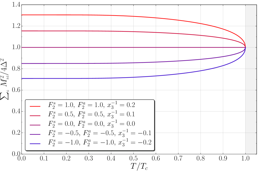
Figure 4: Deviation of the Nambu Sum from polarization corrections to the the $J=2$ Higgs modes of ³He-B for a range of interactions in both the Landau and Cooper channels.

The charge conjugation parity of the Bosonic modes with the same orbital, spin and total angular momentum quantum number is reflected dramatically in the polarization corrections to the masses of the Higgs modes. The $J^{\mbox{\small c}}=2^{-}$ modes couple to a quadrupolar excitation of the Fermionic vacuum, leading to a mass shift from the interaction $F_{2}^{s}$ in the spin-symmetric particle-hole channel, which is generally repulsive except possibly near $p=0\,\mbox{bar}$.Halperin and Varoquaux (1990) By contrast excitation of the $J^{\mbox{\small c}}=2^{+}$ modes is coupled to a quadrupolar spin-polarization, and thus has a polarization correction to its mass from the interaction $F_{2}^{a}$ in the anti-symmetric (exchange) particle-hole channel; this interaction is expected to be attractive at all pressures. In addition, both $J^{\mbox{\small c}}=2^{\pm}$ Higgs modes couple to f-wave pairing fluctuations with the same $J$ and parity c. In this case the asymmetry in the mass shifts for $J^{\mbox{\small c}}=2^{\pm}$ originates from $(\omega/2|\Delta|)^{2}\,x_{3}^{-1}$. Thus, the aysmmetry in the weak-coupling mass spectrum, i.e. $\sqrt{12/5}\Delta$ vs. $\sqrt{8/5}\Delta$, leads to additional asymmetry in the polarization corrections from the f-wave interactions in the Cooper channel. These trends are shown explicitly by the perturbative results in Eqs. 92 and 113. Figure 4 summarizes the magnitude of the corrections to the NSR for a range of interactions in the Landau and Cooper channels. The violation of the NSR onsets rapidly below $T_{c}$, with deviations of order $20-30\%$ for the Fermionic interactions characteristic of normal ³He.

Excitation of the $J^{\mbox{\small c}}=2^{+},m$ modes typically occurs through weakly coupled channels at finite wavelength, $q\neq 0$, as coupling via an external field with symmetry $h_{2,m}^{(1,2)}$ is not easily realized. Koch and Wölfle showed that the weak violation of particle-hole symmetry by the normal-state Fermionic vacuum lifts a selection rule that otherwise prohibits the coupling of the $J^{\mbox{\small c}}=2^{+}$ Higgs modes to density and mass current fluctuations.Koch and Wölfle (1981) Thus, the $J^{\mbox{\small c}}=2^{+},m$ modes can be excited by density and mass current channels, albeit with a coupling that is reduced by the factor, $\zeta\approx k_{\text{B}}T_{c}/E_{f}\ll 1$, the measure of the asymmetry of the spectrum of particle and hole excitations of the normal Fermionic vacuum at $\varepsilon\approx k_{\text{B}}T_{c}$.McKenzie and Sauls This coupling leads to resonant excitation of the $J^{\mbox{\small c}}=2^{+}$ Higgs mode by absorption of zero-sound phonons. Indeed ultra-sound absorption spectroscopy provided the first detection of the Higgs mode in a BCS condensate.Giannetta et al. (1980); Mast et al. (1980) The definitive identification of the absorption resonance as the $J^{\mbox{\small c}}=2^{+}$ Higgs mode was made by Avenel et al. who observed the five-fold Zeeman splitting of the zero-sound absorption resonance in an applied magnetic field.Avenel et al. (1980)

Acoustic spectroscopy provides precision measurements of the mass of the $J^{\mbox{\small c}}=2^{+}$ Higgs mode. The magnitude of the polarization correction to the the $J^{\mbox{\small c}}=2^{+}$ Higgs mass for $T\rightarrow 0$ is measured to be $\delta M_{2^{+}}\approx-0.19\,\Delta$, as shown in Fig. 5, indicating that the interactions giving rise to the mass shift are net attractive. The data are from Ref. Mast et al., 1980 for a pressure of $p=13\,\mbox{bar}$ (yellow diamonds), and from Ref. Avenel et al., 1980 for pressures, $p=0.8-3.5\,\mbox{bar}$ (red squares). Also shown are theoretical results for the polarization correction calculated as a function of temperature. In this case we assumed the most attractive estimate for the exchange interaction, $F_{2}^{a}=-0.88$,Halperin and Varoquaux (1990), which accounts for only half of the measured value of $\delta M_{2^{+}}$. An attractive f-wave interaction, $x_{3}^{-1}\approx-0.2$, in the Cooper channel provides the additional polarization correction. If we use the weaker value of $F_{2}^{a}\simeq-0.37$ reported by the Helium-Three CalculatorHaard (2000) for $p=13\,\mbox{bar}$ we obtain a correspondingly stronger attractive f-wave interaction, $x_{3}^{-1}\simeq-0.35$. An attractive f-wave interaction of similar magnitude, $x_{3}^{-1}\simeq-0.33$ at $p\approx 4.3\,\mbox{bar}$, is also inferred from an analysis of acoustic Faraday rotation of transverse sound that is mediated by the $J^{\mbox{\small c}}=2^{-}$ Higgs mode.Lee et al. (1999); Sauls (2000) Analysis of recent acoustic Faraday rotation measurements, outside the regime of the linear Zeeman splitting of the energy levels of the $J^{\mbox{\small c}}=2^{+},m$ modes, report comparable or smaller values: $x_{3}^{-1}\approx-0.4$ to $x_{3}^{-1}\approx-0.2$.Collett et al. (2013); Davis et al. (2006) A complete and systematic determination of the relevant interactions in the Landau and Cooper channels is possible from the combined measurements of the masses of the $J^{\mbox{\small c}}=2^{\pm}$ modes using longitudinal and transverse sound spectroscopy, combined with measurements of the velocities of zero-sound, first-sound, and the magnetic susceptibilties in both the normal- and superfluid phases of ³He.

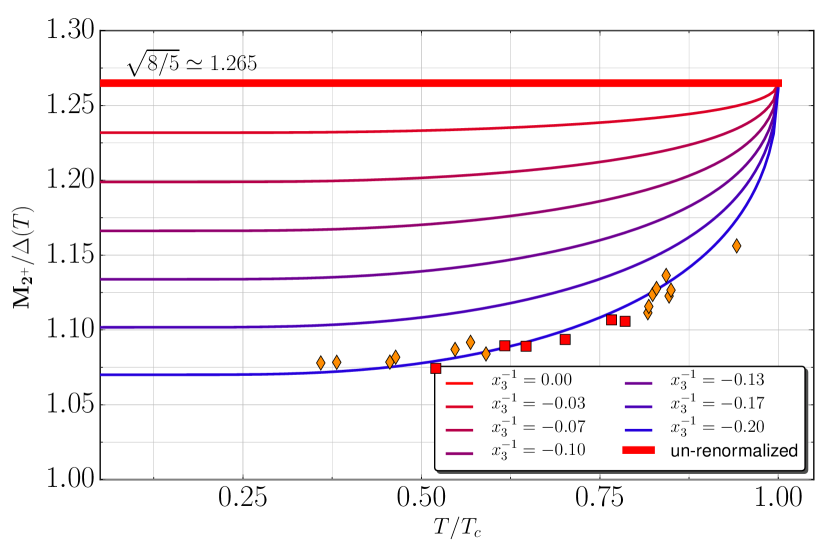
Figure 5: $J^{\mbox{\small c}}=2^{+}$ Higgs Mass. The data are for a pressures of $p=13\,\mbox{bar}$ (yellow diamonds),Mast et al. (1980) and for $p=0.8-3.5\,\mbox{bar}$ (red squares).Avenel et al. (1980) Theoretical calculations of the mass are for $F_{2}^{a}=-0.88$ and values of the f-wave interaction in the Cooper channel given in the legend.

VII.4 Light Higgs Modes in the $J^{\mbox{\small c}}=1^{+}$ Sector

The $J^{\mbox{\small c}}=1^{+}$ mode amplitudes can be related to the parameters of the degeneracy space of relative spin- and orbital rotations, i.e. ${\cal R}[\vartheta{\bf n}]\in{\tt SO(3)}_{\mbox{\footnotesize L-S}}$, where ${\bf n}$ is the axis of rotation, defined by polar and azimuthal angles, and a third variable being angle of rotation, $\vartheta$. The angles define massless NG modes reflecting the spontaneous breaking of separate symmetries under spin- and orbital rotations, i.e. ${\tt SO(3)}_{\mbox{\footnotesize L}}\times{\tt SO(3)}_{\mbox{\footnotesize S}}$. The $J^{\mbox{\small c}}=1^{+}$ multiplet provides a novel example of mass generation corresponding to the “Light Higgs” extension of the standard model in particle physics.Zavjalov et al. (2016) The Light Higgs scenario works as follows: In ³He separate invariance under spin- and orbital rotations is broken by the nuclear dipole-dipole interaction, which acts as weak symmetry breaking perturbation with an energy scale of order $V_{\text{D}}\sim 10^{-7}\,\mbox{K}$ per particle compared to the characteristic two-body interaction energy of order $V\sim 1\,\mbox{K}$. The dipolar energy lifts the degeneracy with respect to separate spin and orbital rotations, which renders the $J^{\mbox{\small c}}=1^{+}$ multiplet a triplet of “pseudo Nambu-Goldstone modes” in which one or more of the NG modes acquires a mass from the weak symmetry breaking field. Long wavelength excitiations of the axis of rotation, ${\bf n}$, remain gapless; however, excitations of the rotation angle, $\vartheta$, acquire a mass gap $M_{\text{LH}}/\hbar$ $=$ $\Omega_{\text{B}}\simeq 10\,\mbox{kHz}\ll 2\Delta/\hbar\simeq 100\,\mbox{MHz}$, where $\Omega_{\text{B}}$ is the longitudinal NMR resonance frequency of ³He-B. An external magnetic field further lifts the degeneracy of the remaining zero mass NG modes which split into an optical magnon with mass, $M_{\text{opt}}=\hbar\gamma B$, and a massless acoustic magnon. A direct detection of the Light Higgs Boson in ³He-B was recently achieved by measuring the decay of optical magnons created by magnetic pumping (a magnon BEC). A sharp threshold for decay of optical magnons to a pair of Light Higgs modes was observed by tuning the mass of the optical magnons on resonance, i.e. $M_{\text{opt}}=\hbar\gamma B\geq 2M_{\text{LH}}=2\hbar\Omega_{\text{B}}$.Zavjalov et al. (2016)

VIII Summary and Outlook

Mass generation based on spontaneous symmetry breaking and the introduction of an internal symmetry (particle-hole symmetry in BCS theory) implies a connection between the masses of the Fermion and Boson excitations of the broken symmetry vacuum state, and a hidden supersymmetry in the class of BCS-NJL theories.Nambu (1985, 1995) Nambu’s proposed sum rule, inspired in part by the Bosonic spectrum of ³He-B, however, is not protected against symmetry breaking perturbations to the broken symmetry vacuum state, including polarization of the vacuum state by excitation of a Higgs boson with symmetry distinct from that of the vacuum. For the case of ³He-B, we show that corrections to the weak-coupling BCS theory and Fermionic interactions combined with vacuum polarization by the Higgs fields, lead to corrections to the masses of the Higgs modes, and in general a violation of the NSR. Our results, as well as other effects of weak perturbations like the nuclear dipolar energy, the Zeeman energy and weak violations of particle-hole symmetry, highlight the roles of symmetry breaking perturbations.

Current research in topological condensed matter addresses the transport properties and spectrum of Fermionic excitations confined near surfaces, interfaces and edges of topological insulators and topological superconductors. Relatively recent theoretical work has shown how supersymmetry can also emerge at the boundary of topological superfluids.Grover et al. (2014) The B-phase of superfluid ³He is the realization of a 3D time-reversal invariant topological superfluid, with a spectrum of helical Majorana Fermions confined on any bounding surface. Thus, a frontier in topological quantum fluids is the role of confinement as a symmetry breaking perturbation on the Bosonic spectrum of confined ³He-B, and the possible signatures of the surface spectrum of Majorana Fermions in the Bosonic modes of confined ³He-B. New studies of the effects of confinement and symmetry-breaking perturbations on both the bulk and surface Bosonic and Fermionic excitations of topological superfluids will hopefully shed new light on the connection between spontaneous symmetry breaking, hidden supersymmetry and topology of the broken symmetry vacuum state in topological superfluids.

IX Acknowledgements

The research of JAS was supported by the National Science Foundation (Grants DMR-1106315 and DMR-1508730). The work of JAS was also carried out in part at the Aspen Center for Physics with partial support by National Science Foundation grant PHY-1066293. The work of T. M. was supported by JSPS (No. JP16K05448) and “Topological Materials Science” (No. JP15H05855) KAKENHI on innovation areas from MEXT. We thank Chandra Varma, Grigory Volovik and Anton Vorontsov for discussions on the spectrum of collective modes in superfluid ³He and unconventional superconductors that informed this work.

X Appendix

X.1 TDGL Effective Potentials

The potentials that enter the TDGL functional that determine the masses of the Bosonic modes are given by $u_{p}=\Delta^{2}\,\bar{u}_{p}$

$$\bar{u}_{1} = \genfrac{}{}{}{1}{4}{3}\mbox{Tr}\Big{\{}{\mathcal{D}}\Big{\}}\mbox{Tr}\Big{\{}{\mathcal{D}}^{*}\Big{\}}+\mbox{Tr}\Big{\{}{\mathcal{D}}{\mathcal{D}}^{\text{tr}}\Big{\}}+\mbox{Tr}\Big{\{}{\mathcal{D}}{\mathcal{D}}^{\text{tr}}\Big{\}}^{*}\,,\qquad$$ (114)

$$\bar{u}_{2} = 2\,\mbox{Tr}\Big{\{}{\mathcal{D}}{\mathcal{D}}^{{\dagger}}\Big{\}}+\genfrac{}{}{}{1}{1}{3}\left(\mbox{Tr}\Big{\{}{\mathcal{D}}\Big{\}}+\mbox{Tr}\Big{\{}{\mathcal{D}}^{*}\Big{\}}\right)^{2}\,,$$ (115)

$$\bar{u}_{3} = \genfrac{}{}{}{1}{1}{3}\left(\mbox{Tr}\Big{\{}{\mathcal{D}}{\mathcal{D}}^{\text{tr}}\Big{\}}+\mbox{Tr}\Big{\{}{\mathcal{D}}{\mathcal{D}}^{\text{tr}}\Big{\}}^{*}\right)$$ (116)

$$+ \genfrac{}{}{}{1}{2}{3}\left(\mbox{Tr}\Big{\{}{\mathcal{D}}{\mathcal{D}}^{{\dagger}}\Big{\}}+\mbox{Tr}\Big{\{}{\mathcal{D}}{\mathcal{D}}^{*}\Big{\}}\right)\,.$$

$$\bar{u}_{4} = \genfrac{}{}{}{1}{4}{3}\mbox{Tr}\Big{\{}{\mathcal{D}}{\mathcal{D}}^{{\dagger}}\Big{\}}+\genfrac{}{}{}{1}{1}{3}\left(\mbox{Tr}\Big{\{}{\mathcal{D}}^{2}\Big{\}}+\mbox{Tr}\Big{\{}{\mathcal{D}}^{2}\Big{\}}^{*}\right)\,,\qquad\qquad$$ (117)

$$\bar{u}_{5} = \genfrac{}{}{}{1}{1}{3}\left(\mbox{Tr}\Big{\{}{\mathcal{D}}{\mathcal{D}}^{{\dagger}}\Big{\}}+\mbox{Tr}\Big{\{}{\mathcal{D}}{\mathcal{D}}^{{\dagger}}\Big{\}}^{*}\right)$$ (118)

$$+ \genfrac{}{}{}{1}{1}{3}\left(\mbox{Tr}\Big{\{}{\mathcal{D}}^{\text{tr}}{\mathcal{D}}\Big{\}}+\mbox{Tr}\Big{\{}{\mathcal{D}}^{\text{tr}}{\mathcal{D}}\Big{\}}^{*}\right)+\genfrac{}{}{}{1}{2}{3}\mbox{Tr}\Big{\{}{\mathcal{D}}{\mathcal{D}}^{*}\Big{\}}\,.$$

Note that these potentials are defined relative to the BW ground state, and thus invariant only under ${\tt SO(3)}_{\mbox{\footnotesize J}}\times{\tt T}$.

X.2 Symmetry Relations

The components of the $4\times 4$ Nambu propagator are related by fundamental symmetries with respect to (i) permutation exchange symmetry and (ii) conjugation symmetry. These symmetries imply the following relations between the components of the quasiclassical propagator,

X.2.1 Exchange symmetry

$$g^{\prime}(\hat{p},\varepsilon_{n};{\bf q},\omega_{m}) = +g(-\hat{p},-\varepsilon_{n};{\bf q},\omega_{m})\,,$$ (119)

$$\vec{g}^{\prime}(\hat{p},\varepsilon_{n};{\bf q},\omega_{m}) = +\vec{g}(-\hat{p},-\varepsilon_{n};{\bf q},\omega_{m})\,,$$ (120)

$$f(\hat{p},\varepsilon_{n};{\bf q},\omega_{m}) = +f(-\hat{p},-\varepsilon_{n};{\bf q},\omega_{m})\,,$$ (121)

$$\vec{f}(\hat{p},\varepsilon_{n};{\bf q},\omega_{m}) = -\vec{f}(-\hat{p},-\varepsilon_{n};{\bf q},\omega_{m})\,,$$ (122)

as well as for the mean-field self energies,

$$\Sigma^{\prime}(\hat{p};{\bf q},\omega_{m}) = +\Sigma(-\hat{p};{\bf q},\omega_{m})\,,$$ (123)

$$\vec{\Sigma}^{\prime}(\hat{p};{\bf q},\omega_{m}) = +\vec{\Sigma}(-\hat{p};{\bf q},\omega_{m})\,,$$ (124)

$$d(\hat{p};{\bf q},\omega_{m}) = +d(-\hat{p};{\bf q},\omega_{m})\,,$$ (125)

$$\vec{d}(\hat{p};{\bf q},\omega_{m}) = -\vec{d}(-\hat{p};{\bf q},\omega_{m})\,.$$ (126)

Note that Eqs. 125 and 126 reflect the fact that spin-singlet Cooper pairs have even parity, while spin-triplet pairs are odd-parity.

X.2.2 Conjugation symmetry

The conjugation symmetry relations follow from complex conjugation of the two-point functions.

$$g^{\prime}(\hat{p},\varepsilon_{n};{\bf q},\omega_{m}) = +g(-\hat{p},\varepsilon_{n};-{\bf q},\omega_{m})^{*}\,,$$ (127)

$$\vec{g}^{\prime}(\hat{p},\varepsilon_{n};{\bf q},\omega_{m}) = +\vec{g}(-\hat{p},\varepsilon_{n};-{\bf q},\omega_{m})^{*}\,,$$ (128)

$$f^{\prime}(\hat{p},\varepsilon_{n};{\bf q},\omega_{m}) = +f(-\hat{p},\varepsilon_{n};-{\bf q},\omega_{m})^{*}\,,$$ (129)

$$\vec{f}^{\prime}(\hat{p},\varepsilon_{n};{\bf q},\omega_{m}) = -\vec{f}(-\hat{p},\varepsilon_{n};-{\bf q},\omega_{m})^{*}\,.$$ (130)

$$\Sigma^{\prime}(\hat{p};{\bf q},\omega_{m}) = +\Sigma(-\hat{p};-{\bf q},\omega_{m})^{*}\,,$$ (131)

$$\vec{\Sigma}^{\prime}(\hat{p};{\bf q},\omega_{m}) = +\vec{\Sigma}(-\hat{p};-{\bf q},\omega_{m})^{*}\,,$$ (132)

$$d^{\prime}(\hat{p};{\bf q},\omega_{m}) = +d(-\hat{p};-{\bf q},\omega_{m})^{*}\,,$$ (133)

$$\vec{d}^{\prime}(\hat{p};{\bf q},\omega_{m}) = -\vec{d}(-\hat{p};-{\bf q},\omega_{m})^{*}\,.$$ (134)

X.3 Dynamical Equations

$$\vec{d}^{(-)}(\hat{p};{\bf q},\omega) = \int\frac{d\Omega_{p^{\prime}}}{4\pi}\,V^{(1)}(\hat{p},\hat{p}^{\prime})\,\Big{\{}\left[\frac{\mbox{\small 1}}{\mbox{\small 2}}\gamma+\frac{\mbox{\small 1}}{\mbox{\small 4}}(\omega^{2}-\eta^{\prime 2}-4|\vec{\Delta}(\hat{p}^{\prime})|^{2})\bar{\lambda}(\hat{p}^{\prime})\right]\,\vec{d}^{(-)}(\hat{p}^{\prime})+\bar{\lambda}(\hat{p}^{\prime})\vec{\Delta}(\hat{p}^{\prime})\,(\vec{\Delta}(\hat{p}^{\prime})\cdot\vec{d}^{(-)}(\hat{p}^{\prime}))$$ (135)

$$\hskip 85.35826pt-\frac{\mbox{\small 1}}{\mbox{\small 2}}\eta^{\prime}\,\bar{\lambda}(\hat{p}^{\prime})\,\vec{\Delta}(\hat{p}^{\prime})\,\Sigma^{(-)}(\hat{p}^{\prime})-\frac{\mbox{\small 1}}{\mbox{\small 2}}\omega\,\bar{\lambda}(\hat{p}^{\prime})\,\vec{\Delta}(\hat{p}^{\prime})\,\Sigma^{(+)}(\hat{p}^{\prime})\Big{\}}\,,$$

$$\vec{d}^{(+)}(\hat{p};{\bf q},\omega) = \int\frac{d\Omega_{p^{\prime}}}{4\pi}\,V^{(1)}(\hat{p},\hat{p}^{\prime})\,\Big{\{}\left[\frac{\mbox{\small 1}}{\mbox{\small 2}}\gamma+\frac{\mbox{\small 1}}{\mbox{\small 4}}(\omega^{2}-\eta^{\prime 2})\bar{\lambda}(\hat{p}^{\prime})\right]\,\vec{d}^{(+)}(\hat{p}^{\prime})-\bar{\lambda}(\hat{p}^{\prime})\vec{\Delta}(\hat{p}^{\prime})(\vec{\Delta}(\hat{p}^{\prime})\cdot\vec{d}^{(+)}(\hat{p}^{\prime}))$$ (136)

$$\hskip 85.35826pt+\genfrac{}{}{}{1}{i}{2}\eta^{\prime}\,\bar{\lambda}(\hat{p}^{\prime})\,\vec{\Delta}(\hat{p}^{\prime})\times\vec{\Sigma}^{(-)}(\hat{p}^{\prime})+\genfrac{}{}{}{1}{i}{2}\omega\,\bar{\lambda}(\hat{p}^{\prime})\,\vec{\Delta}(\hat{p}^{\prime})\times\vec{\Sigma}^{(+)}(\hat{p}^{\prime})\Big{\}}\,,$$

$$\Sigma^{(+)}(\hat{p};{\bf q},\omega) = \Sigma^{(+)}_{\text{ext}}(\hat{p})+\int\frac{d\Omega_{p^{\prime}}}{4\pi}\,A^{s}(\hat{p},\hat{p}^{\prime})\,\Big{[}\left(\frac{\omega^{2}}{\omega^{2}-\eta^{\prime 2}}\right)\,\left(1-\lambda(\hat{p}^{\prime})\right)\,\Sigma^{(+)}(\hat{p}^{\prime})+\left(\frac{\omega\eta^{\prime}}{\omega^{2}-\eta^{\prime 2}}\right)\,\left(1-\lambda(\hat{p}^{\prime})\right)\Sigma^{(-)}(\hat{p}^{\prime})$$ (137)

$$\hskip 113.81102pt+\frac{\mbox{\small 1}}{\mbox{\small 2}}\omega\,\bar{\lambda}(\hat{p}^{\prime})\,\vec{\Delta}(\hat{p}^{\prime})\cdot\vec{d}^{(-)}(\hat{p}^{\prime})\Big{]}$$

$$\Sigma^{(-)}(\hat{p};{\bf q},\omega) = \Sigma^{(-)}_{\text{ext}}(\hat{p})+\int\frac{d\Omega_{p^{\prime}}}{4\pi}\,A^{s}(\hat{p},\hat{p}^{\prime})\,\Big{[}\left(\frac{\omega\eta^{\prime}}{\omega^{2}-\eta^{\prime 2}}\right)\,\left(1-\lambda(\hat{p}^{\prime})\right)\Sigma^{(+)}(\hat{p}^{\prime})+\Big{\{}1+\left(\frac{\eta^{\prime 2}}{\omega^{2}-\eta^{\prime 2}}\right)\,\left(1-\lambda(\hat{p}^{\prime})\right)\Big{\}}\,\Sigma^{(-)}(\hat{p}^{\prime})$$ (138)

$$\hskip 113.81102pt+\frac{\mbox{\small 1}}{\mbox{\small 2}}\eta^{\prime}\,\bar{\lambda}(\hat{p}^{\prime})\,\vec{\Delta}(\hat{p}^{\prime})\cdot\vec{d}^{(-)}(\hat{p}^{\prime})\Big{]}$$

$$\vec{\Sigma}^{(+)}(\hat{p};{\bf q},\omega) = \vec{\Sigma}^{(+)}_{\text{ext}}(\hat{p})+\int\frac{d\Omega_{p^{\prime}}}{4\pi}\,A^{a}(\hat{p},\hat{p}^{\prime})\,\Big{[}\left(\frac{\omega^{2}}{\omega^{2}-\eta^{\prime 2}}\right)\,\left(1-\lambda(\hat{p}^{\prime})\right)\,\vec{\Sigma}^{(+)}(\hat{p}^{\prime})+\bar{\lambda}(\hat{p}^{\prime})\left(\vec{\Delta}(\hat{p}^{\prime})\cdot\vec{\Sigma}^{(+)}(\hat{p}^{\prime})\right)\vec{\Delta}(\hat{p}^{\prime})$$ (139)

$$\hskip 113.81102pt+\left(\frac{\omega\eta^{\prime}}{\omega^{2}-\eta^{\prime 2}}\right)\,\left(1-\lambda(\hat{p}^{\prime})\right)\vec{\Sigma}^{(-)}(\hat{p}^{\prime})\quad-\genfrac{}{}{}{1}{i}{2}\omega\,\bar{\lambda}(\hat{p}^{\prime})\,\vec{\Delta}(\hat{p}^{\prime})\times\vec{d}^{(+)}(\hat{p}^{\prime})\Big{]}$$

$$\vec{\Sigma}^{(-)}(\hat{p};{\bf q},\omega) = \vec{\Sigma}^{(-)}_{\text{ext}}(\hat{p})+\int\frac{d\Omega_{p^{\prime}}}{4\pi}\,A^{a}(\hat{p},\hat{p}^{\prime})\,\Big{[}\Big{\{}1+\left(\frac{\eta^{\prime 2}}{\omega^{2}-\eta^{\prime 2}}\right)\,\left(1-\lambda(\hat{p}^{\prime})\right)\Big{\}}\,\vec{\Sigma}^{(-)}(\hat{p}^{\prime})-\bar{\lambda}(\hat{p}^{\prime})\left(\vec{\Delta}(\hat{p}^{\prime})\cdot\vec{\Sigma}^{(-)}(\hat{p}^{\prime})\right)\vec{\Delta}(\hat{p}^{\prime})$$ (140)

$$\hskip 113.81102pt+\left(\frac{\omega\eta^{\prime}}{\omega^{2}-\eta^{\prime 2}}\right)\,\left(1-\lambda(\hat{p}^{\prime})\right)\vec{\Sigma}^{(+)}(\hat{p}^{\prime})\quad-\genfrac{}{}{}{1}{i}{2}\eta^{\prime}\,\bar{\lambda}(\hat{p}^{\prime})\,\vec{\Delta}(\hat{p}^{\prime})\times\vec{d}^{(+)}(\hat{p}^{\prime})\Big{]}\,,$$

where $\eta^{\prime}\equiv{\bf v}_{\hat{p}^{\prime}}\cdot{\bf q}$ and the Tsuneto function, $\lambda(\hat{p}^{\prime})\equiv\lambda(\eta^{\prime},\omega;|\Delta(\hat{p}^{\prime})|)$, for ${\bf q}\neq 0$ is given by Eq. (62) of Ref. Moores and Sauls, 1993. The particle-particle interaction vertex in the spin-triplet channel is parametrized by an interaction parameter, $v_{\ell}$, for each odd-parity angular momentum channel, as in Eq. 33. In the case of the particle-hole interaction vertex, the functions $A^{s,a}(\hat{p},\hat{p}^{\prime})$ are the forward scattering amplitudes for spin-independent ($A^{s}$) and spin-exchange ($A^{a}$) scattering of quasiparticles with momenta near the Fermi surface. These amplitudes are related to the the Landau interactions, $F^{s,a}(\hat{p},\hat{p}^{\prime})$, by the integral equation,

$$A^{s,a}(\hat{p},\hat{p}^{\prime})=F^{s,a}(\hat{p},\hat{p}^{\prime})-\int\frac{d\Omega_{p^{\prime\prime}}}{4\pi}F^{s,a}(\hat{p},\hat{p}^{\prime\prime})\,A^{s,a}(\hat{p}^{\prime\prime},\hat{p}^{\prime})\,.$$ (141)

The standard parametrization of the Landau interaction function in terms of the Landau parameters is $F^{s,a}(\hat{p},\hat{p}^{\prime})=\sum_{\ell\geq 0}\,F^{s,a}_{\ell}\,P_{\ell}(\hat{p}\cdot\hat{p}^{\prime})$.

References

- Nambu and Jona-Lasinio (1961) Y. Nambu and G. Jona-Lasinio, Dynamical Model of Elementary Particles Based on an Analogy with Superconductivity. I, Phys. Rev. 122, 345 (1961).
- Anderson (1963) P. W. Anderson, Plasmons, Gauge Invariance, and Mass, Phys. Rev. 130, 439 (1963).
- Higgs (1964) P. W. Higgs, Broken Symmetries and the Masses of Gauge Bosons, Phys. Rev. Lett. 13, 508 (1964).
- Anderson (1958a) P. W. Anderson, Random-Phase Approximation in the Theory of Superconductivity, Phys. Rev. 112, 1900 (1958a).
- Bogoliubov (1958) N. N. Bogoliubov, New Method in the Theory of Superconductivity, Zh. Eskp. Teor. Fiz. 34, 58 (1958), [english: Sov. Phys. JETP 7, 41-46 (1958)].
- Valatin (1958) J. G. Valatin, Comments on the Theory of Superconductivity, Nuovo Cimento 7, 843 (1958).
- Anderson (1958b) P. W. Anderson, Coherent Excited States in the Theory of Superconductivity: Gauge Invariance and the Meissner Effect, Phys. Rev. 110, 827 (1958b).
- Nambu (2009) Y. Nambu, Nobel Lecture: Spontaneous symmetry breaking in particle physics: A case of cross fertilization, Rev. Mod. Phys. 81, 1015 (2009).
- Littlewood and Varma (1981) P. Littlewood and C. Varma, Gauge-Invariant Theory of the Dynamical Interaction of Charge Density Waves and Superconductivity, Phys. Rev. Lett. 47, 811 (1981).
- Serene (1983) J. W. Serene, in Quantum Fluids and Solids -1983, Vol. 103 (A.I.P., New York, 1983) p. 305.
- Sauls and McKenzie (1991) J. A. Sauls and R. H. McKenzie, Parametric excitation of the modes by zero sound in superfluid 3He-B, Physica B 169, 170 (1991).
- Nambu (1985) Y. Nambu, Fermion-Boson relations in BCS-type theories, Physica D: Nonlinear Phenomena 15, 147 (1985).
- McKenzie and Sauls (1993) R. H. McKenzie and J. A. Sauls, Comment on the coupling of zero sound to the modes of 3He-B, J. Low Temp. Phys. 90, 337 (1993).
- Vdovin (1963) Y. A. Vdovin, in Methods of Quantum Field Theory to the Many Body Problem (Gosatomizdat, Moscow, 1963) pp. 94–109.
- Maki (1974) K. Maki, Propagation of Zero Sound in the Balian-Werthamer State, J. Low Temp. Phys. 16, 465 (1974).
- Wölfle (1976) P. Wölfle, Theory of Sound Propagation in Pair-Correlated Fermi Liquids: Application to 3He-B, Phys. Rev. B 14, 89 (1976).
- Brusov and Popov (1980) P. N. Brusov and V. N. Popov, Non-phonon branches of the Bose spectrum in the B-phase of systems of the 3He type, Zh. Eskp. Teor. Fiz. 78, 2419 (1980), [english: Sov. Phys. JETP 51 (6), 1217-1222 (1980)].
- Volovik and Zubkov (2013) G. E. Volovik and M. A. Zubkov, Nambu sum rule and the relation between the masses of composite Higgs bosons, Phys. Rev. D 87, 075016 (2013).
- Nambu (1995) Y. Nambu, Supersymmetry and Superconductivity, in Broken Symmetry, Selected Papers of Y. Nambu, Vol. World Scientific Series in 20th Century Physics, Vol. 13 (World Scientific, 1995) pp. 390–398.
- Volovik and Zubkov (2014) G. Volovik and M. Zubkov, Higgs Bosons in Particle Physics and in Condensed Matter, J. Low Temp. Phys. 175, 486 (2014).
- Mermin and Stare (1973) N. D. Mermin and G. Stare, Ginzburg-landau approach to pairing, Phys. Rev. Lett. 30, 1135 (1973).
- Brinkman and Anderson (1973) W. F. Brinkman and P. W. Anderson, Anisotropic Superfluidity in 3He: Consequences of the Spin-Fluctuation Model, Phys. Rev. A8, 2732 (1973).
- Leggett (1975) A. J. Leggett, Theoretical Description of the New Phases of Liquid 3He, Rev. Mod. Phys. 47, 331 (1975).
- Rainer and Serene (1976) D. Rainer and J. W. Serene, Free Energy of Superfluid , Phys. Rev. B 13, 4745 (1976).
- Serene and Rainer (1983) J. W. Serene and D. Rainer, The Quasiclassical Approach to , Phys. Rep. 101, 221 (1983).
- Ali et al. (2011) S. Ali, L. Zhang, and J. A. Sauls, Thermodynamic Potential for Superfluid 3He in Silica Aerogel, J. Low Temp. Phys. 162, 233 (2011).
- Sauls and Serene (1981a) J. A. Sauls and J. W. Serene, Potential Scattering Models for the Quasiparticle Interactions in Liquid 3He, Phys. Rev. B 24, 183 (1981a).
- Volovik and Khazan (1984) G. E. Volovik and M. V. Khazan, Effect of textures on the collective modes in 3He-B, Zh. Eskp. Teor. Fiz. 87, 583 (1984), [english: Sov. Phys. JETP 60, 276 (1984)].
- Theodorakis (1988) S. Theodorakis, Lagrangian of superfluid 3He, Phys. Rev. B 37, 3318 (1988).
- Volovik (1984) G. E. Volovik, Unusual Splitting of the Spectrum of Collective Modes in Superfluid 3He-B, Pis’ma Zh. Eskp. Teor. Fiz. 39, 304 (1984), [english: 39, 365 (1984)].
- Fishman and Sauls (1988a) R. S. Fishman and J. A. Sauls, Doublet Splitting and Low-Field Evolution of the Real Squashing Modes in Superfluid -B, Phys. Rev. Lett. 61, 2871 (1988a).
- Popov (1987) V. N. Popov, Functional Integrals and Collective Excitations, cambridge monographs on mathematical physics ed. (Cambridge University Press, Cambridge, UK, 1987).
- Serene (1974) J. W. Serene, Theory of Collisionless Sound in Superfluid 3He, Ph.D. thesis, Cornell University (1974).
- Wölfle (1977) P. Wölfle, Collisionless collective modes in superfluid , Physica 90B, 96 (1977).
- Sauls (2000) J. A. Sauls, Broken Symmetry and Non-Equilibrium Superfluid 3He, in Topological Defects and Non-Equilibrium Symmetry Breaking Phase Transitions - Lecture Notes for the 1999 Les Houches Winter School, edited by H. Godfrin and Y. Bunkov (Elsievier Science Publishers, Amsterdam, 2000) pp. 239–265, http://arxiv.org/abs/cond-mat/9910260 .
- Choi et al. (2007) H. Choi, J. P. Davis, J. Pollanen, T. Haard, and W. Halperin, Strong coupling corrections to the Ginzburg-Landau theory of superfluid 3He, Phys. Rev. B 75, 174503 (2007).
- Wölfle (1974) P. Wölfle, Collisionless Collective Modes in Superfluid 3He, Phys. Lett. 47A, 224 (1974).
- Tewordt and Schopohl (1979) L. Tewordt and N. Schopohl, Gap Parameters and Collective Modes for 3He-B in the Presence of a Strong Magnetic Field, J. Low Temp. Phys. 37, 421 (1979).
- Sauls and Serene (1981b) J. A. Sauls and J. W. Serene, Coupling of Order-Parameter Modes with to Zero Sound in 3He-B, Phys. Rev. B 23, 4798 (1981b).
- Moores and Sauls (1993) G. F. Moores and J. A. Sauls, Transverse Waves in Superfluid 3He-B, J. Low Temp. Phys. 91, 13 (1993).
- (41) R. H. McKenzie and J. A. Sauls, Collective Modes and Nonlinear Acoustics in Superfluid -B, in Helium Three, edited by edited by W. P. Halperin and L. P. Pitaevskii (Elsevier Science Publishers, Amsterdam) p. 255, 1309.6018 .
- McKenzie and Sauls (2013) R. H. McKenzie and J. A. Sauls, Collective Modes and Nonlinear Acoustics in Superfluid -B, arXiv 1309.6018, 62 (2013).
- Gorkov (1958) L. P. Gorkov, On the Energy Spectrum on Superconductors, Zh. Eskp. Teor. Fiz. 34, 735 (1958), english: Sov. Phys. JETP, 7, 505-508 (1958).
- Eilenberger (1968) G. Eilenberger, Transformation of Gorkov’s Equation for Type II Superconductors into Transport-Like Equations, Zeit. f. Physik 214, 195 (1968).
- Sauls (1986) J. A. Sauls, F-wave correlations in superfluid 3He, Phys. Rev. B 34, 4861 (1986).
- Keldysh (1965) L. V. Keldysh, Diagram technique for nonequilibrium processes, Zh. Eskp. Teor. Fiz. 47, 1515 (1965), english: Sov. Phys. JETP, 20, 1018 (1965).
- Tsuneto (1960) T. Tsuneto, Transverse collective excitations in superconductors and electromagnetic absorption, Phys. Rev. 118, 1029 (1960).
- Layzer and Fay (1974) A. Layzer and D. Fay, Spin fluctuation exchange: Mechanism for a superfluid transition in liquid 3He, Sol. State Comm. 15, 599 (1974).
- Fay (1975) D. Fay, On the application of spin-fluctuation theory to superfluid 3He, Physics Letters A 51, 365 (1975).
- Haard (2000) T. Haard, 3He Calculator, ULT@Northwestern Online (2000).
- Halperin and Varoquaux (1990) W. P. Halperin and E. Varoquaux, in Helium Three, edited by W. P. Halperin and L. P. Pitaevskii (Elsevier Science Publishers, Amsterdam, 1990) p. 353.
- Lee et al. (1999) Y. Lee, T. Haard, W. Halperin, and J. A. Sauls, Discovery of an Acoustic Faraday Effect in Superfluid 3He-B, Nature 400, 431 (1999).
- Collett et al. (2013) C. A. Collett, J. Pollanen, J. I. A. Li, W. J. Gannon, and W. P. Halperin, Nonlinear field dependence and -wave interactions in superfluid 3He, Phys. Rev. B 87, 024502 (2013).
- Fishman and Sauls (1986) R. S. Fishman and J. A. Sauls, Response Functions and Collective Modes of Superfluid -B in Strong Magnetic Fields, Phys. Rev. B 33, 6068 (1986).
- Hoyt et al. (1981) R. F. Hoyt, H. N. Scholtz, and D. O. Edwards, Superfluid 3He-B: The dependence of the susceptibility and energy gap on magnetic field, Physica B+C 107, 287 (1981).
- Fishman and Sauls (1988b) R. S. Fishman and J. A. Sauls, Response Functions and Collective Modes of Superfluid -B in Strong Magnetic Fields: Determination of Materials Parameters From Experiments, Phys. Rev. B 38, 2526 (1988b).
- Baym and Pethick (1991) G. Baym and C. J. Pethick, Landau Fermi-Liquid Theory (Wiley, New York, 1991).
- Koch and Wölfle (1981) V. E. Koch and P. Wölfle, Coupling of New Order Parameter Collective Modes to Sound Waves in Superfluid 3He, Phys. Rev. Lett. 46, 486 (1981).
- Giannetta et al. (1980) R. W. Giannetta, A. Ahonen, E. Polturak, J. Saunders, and E. K. Zeise, Observation of a New Sound Attenuation Peak in Superfliud 3He-B, Phys. Rev. Lett. 45, 262 (1980).
- Mast et al. (1980) D. B. Mast, B. K. Sarma, J. R. Owers-Bradley, I. D. Calder, J. B. Ketterson, and W. P. Halperin, Measurements of High Frequency Sound Propagation in 3He-B, Phys. Rev. Lett. 45, 266 (1980).
- Avenel et al. (1980) O. Avenel, E. Varoquaux, and H. Ebisawa, Field Splitting of the New Sound Attenuation Peak in 3He-B, Phys. Rev. Lett. 45, 1952 (1980).
- Davis et al. (2006) J. P. Davis, H. Choi, J. Pollanen, and W. P. Halperin, Collective Modes and f-Wave Pairing Interactions in Superfluid 3He, Phys. Rev. Lett. 97, 115301 (2006).
- Zavjalov et al. (2016) V. V. Zavjalov, S. Autti, V. B. Eltsov, P. J. Heikkinen, and G. E. Volovik, Light Higgs channel of the resonant decay of magnon condensate in superfluid 3He-B, Nature Comm. 7, 10294 (2016).
- Grover et al. (2014) T. Grover, D. N. Sheng, and A. Vishwanath, Emergent Space-Time Supersymmetry at the Boundary of a Topological Phase, Science 344, 280 (2014).