Imposing various boundary conditions on positive definite kernels

Abstract

This work is motivated by the frequent occurrence of boundary value problems with various boundary conditions in the modeling of some problems in engineering and physical science. Here we propose a new technique to force the positive definite kernels such as some radial basis functions to satisfy the boundary conditions exactly. It can improve the applications of existing methods based on positive definite kernels and radial basis functions especially the pseudospectral radial basis function method for handling the differential equations with more complicated boundary conditions. The proposed method is applied to a singularly perturbed steady-state convection-diffusion problem, two and three dimensional Poisson’s equations with various boundary conditions.

, , ,

1 Introduction

Setting up and solving models described by the Poisson’s equation is one of the cornerstones of electrostatics. The Poisson’s equations combined with the various type of boundary conditions are of importance for a wide field of applications in electrostatics, mechanical engineering, theoretical and computational physics and theoretical chemistry. This work is motivated by the frequent occurrence of boundary value problems with various boundary conditions in the modeling of some problems in engineering and physical science. In recent years, several kernel based algorithms have been proposed for solving boundary value problems [1, 2, 3, 4, 5, 6, 7, 8, 9, 10, 11, 12, 13, 14, 15, 16, 17, 18, 19, 20, 21, 22, 23, 24, 25]. Fasshauer [25] has shown that many of the standard algorithms and strategies used for solving ordinary and partial differential equations with polynomial pseudospectral methods can be easily adapted for the use with radial basis functions. pseudospectral radial basis function (RBF–PS) method has already been proven successful in numerical solution of various type of differential equation [25, 26, 27, 28, 29, 30, 31, 32, 33]. This paper presents a new approach to imposing various boundary conditions on positive definite kernels such as some radial basis functions and their application in kernel based pseudospectral method. The various boundary conditions such as Dirichlet, Neumann, Robin, mixed and multi–point boundary conditions, have been considered. Here we propose a new technique to force the radial basis functions to satisfy the boundary conditions exactly, so the approximate solution also satisfies the boundary conditions exactly. It can improve the applications of existing methods based on positive definite kernels and radial basis functions especially the pseudospectral radial basis function method for handling the differential equations with more complicated boundary conditions. Some new kernels are constructed using general kernels in a manner which satisfies required conditions and we prove that if the reference kernel is positive definite then the newly constructed kernel is positive definite, also. Furthermore, we show that the collocation matrix is nonsingular if some conditions are satisfied. In [25] RBF–PS method has been applied successfully to homogeneous Dirichlet boundary conditions. Here we try to handle many other types of boundary conditions in one, two and three dimension. The proposed technique can be applied to other kinds of radial basis functions methods easily. Imposing boundary conditions is a key issue in meshless methods based on radial basis functions and can be quite challenging. We shall discuss how to deal with boundary conditions in radial basis functions methods. The Dirichlet boundary condition is relatively easy and other type boundary conditions require more attentions. There are two basic approaches to deal with boundary conditions for pseudospectral methods, restrict the method to basis functions that satisfy the boundary conditions or add some additional equations to enforce the boundary conditions. An inherent advantage of the proposed technique is its simplicity and easy programmability. Difficulties in the various radial basis function method arise in applying the method to a boundary value problem with more complicated nonhomogeneous boundary conditions in each dimension such as:
Let $u$ be the solution which we are looking for and $\Omega=[a,b]$ is the domain of problem in one direction:

$1.$ the Dirichlet boundary condition

$$u(a)=A\hskip 28.45274ptand\hskip 28.45274ptu(b)=B,$$ (1.1)

$2.$ the Neumann boundary condition

$$u^{\prime}(a)=A\hskip 28.45274ptand\hskip 28.45274ptu^{\prime}(b)=B,$$ (1.2)

$3.$ the mixed boundary condition

$$u(a)=A\hskip 28.45274ptand\hskip 28.45274ptu^{\prime}(b)=B,$$ (1.3)

$4.$ the Robin boundary condition

$$\begin{array}[]{ll}\alpha_{1}u(a)+\beta_{1}u^{\prime}(a)&=c_{1},\\ \alpha_{2}u(b)+\beta_{2}u^{\prime}(b)&=c_{1},\\ \end{array}$$ (1.4)

$5.$ the Multi–point boundary condition

$$u(a)=\sum_{j=1}^{J}\alpha_{j}u(\xi_{j})+\psi,$$ (1.5)

where

$$a<\xi_{1}<\xi_{2}<...<\xi_{J}<b.$$

In fact, the Dirichlet and Neumann boundary conditions are special cases of the Robin boundary condition. The presented technique is easy to utilize by existing radial basis function method for handling more complicated boundary conditions. Several test examples are presented to demonstrate the accuracy and versatility of the proposed technique. We apply it to some problems in one, two and three dimensional with the different type of boundary conditions and compare the results with the RBF collocation method introduced in [25] and the best reported results in the literature. The reported results show that the proposed method is accurate and significantly more efficient than RBF collocation method and some other existing radial basis functions method.

2 Kernel based pseudospectral method

In this section, we give a brief review of the pseudospectral method based on kernels. An important feature of pseudospectral methods is the fact that one usually is content with obtaining an approximation to the solution on a discrete set of grid points. In pseudospectral methods we usually seek an approximate solution of differential equation in the form

$$u_{N}(x)=\sum_{j=1}^{N}\lambda_{j}\phi_{j}(x).$$ (2.6)

For the grid points $x_{i},i=1,...,N,$ We will use the basis functions $\phi_{j}(x)=R(x,x_{j}),$ where $R(x,y)$ is a kernel. If we evaluate the unknown function $u(x)$ at grid points $x_{i},i=1,...,N,$ then we have,

$$u_{N}(x_{i})=\sum_{j=1}^{N}\lambda_{j}\phi_{j}(x_{i}),\hskip 28.45274pti=1,...,N,$$ (2.7)

or in matrix notation,

$$\boldsymbol{u}=A\boldsymbol{\lambda},$$ (2.8)

where $\boldsymbol{\lambda}=[\lambda_{1},...,\lambda_{N}]^{T}$ is the coefficient vector, the evaluation matrix $A$ has the entries $A_{i,j}=\phi_{j}(x_{i})=R(x_{i},x_{j})$ and $\boldsymbol{u}=[u_{N}(x_{1},...,u_{N}(x_{N})]^{T}$. Let $\mathcal{L}$ be a linear operator, we can use the expansion (2.6) to compute the $\mathcal{L}u_{N}$ by operating $\mathcal{L}$ on the basis functions,

$$\mathcal{L}u_{N}=\sum_{j=1}^{N}\beta_{j}\mathcal{L}\phi_{j}(x),\hskip 28.45274ptx\in\mathbb{R}^{d}.$$ (2.9)

If we again evaluate at the grid points $x_{i},i=1,...,N,$ then we get in matrix notation,

$$\boldsymbol{L}\boldsymbol{u}=A_{L}\boldsymbol{\lambda},$$ (2.10)

where $\boldsymbol{u}$ and $\boldsymbol{\lambda}$ are as above and the matrix $A_{L}$ has entries $\mathcal{L}\phi_{j}(x_{i})$. Then we can use (2.8) to solve the coefficient vector $\boldsymbol{\lambda}=A^{-1}\boldsymbol{u},$ and then (2.10) yields,

$$\boldsymbol{L}\boldsymbol{u}=A_{L}A^{-1}\boldsymbol{u},$$ (2.11)

so that the operational matrix $\boldsymbol{L}$ corresponding to linear operator $L$ is given by,

$$\boldsymbol{L}=A_{L}A^{-1}.$$ (2.12)

In order to obtain the differentiation matrix $\boldsymbol{L}$ we need to ensure invertibility of the evaluation matrix $A$. This generally depends both on the basis functions chosen as well as the location of the grid points $x_{i},i=0,...,n$. For positive definite kernels the invertibility of the evaluation matrix $A$ for any set of distinct grid points is guaranteed. Suppose we have a linear differential equation of the form

$$\mathcal{L}u=f,$$ (2.13)

by ignoring boundary conditions. An approximate solution at the grid points can be obtained by solving the discrete linear system

$$\textbf{L}\textbf{u}=\textbf{f},$$ (2.14)

where u and f contain the value of $u$ and $f$ at grid points and L is the mentioned operational matrix corresponds to linear differential operator $\mathcal{L}$. Imposing boundary conditions in radial basis functions methods based on radial basis functions and can be quite challenging. Here we impose boundary conditions on basis functions, instead of add some additional equations in (2.14) to enforce the boundary conditions. Many radial basis functions are defined by a constant called the shape parameter. The choice of shape parameter have a significant impact on the accuracy of an radial basis function method. It is clear that selecting optimal shape parameter in the methods based on the radial basis functions is an open problem. But authors of [29] proposed an algorithm for choosing an optimal value of the shape parameter. Here we consider the effect of different shape parameters on the accuracy of approximations and compare it with the RBF collocation method.

3 Imposing the boundary conditions

For some nonhomogeneous problems, we can construct a homogenization function $M$, which satisfies the nonhomogeneous boundary conditions of problem. Then the nonhomogeneous problem can be reduced to a homogeneous problem as follows. Let

$$\mathcal{L}u(\textbf{x})=f(\textbf{x}),\hskip 14.22636pt\textbf{x}\in\Omega\subset R^{d},\ \mathcal{B}u(\textbf{x})=g(\textbf{x}),\hskip 14.22636pt\textbf{x}\in\partial\Omega$$

where $\partial\Omega$ is the boundary of $\Omega$ and $\mathcal{L}$ is a differential operator. Then the boundary conditions can be homogenized using

$$u(\textbf{x})=v(\textbf{x})+M(\textbf{x}).$$

After homogenization of the boundary conditions, the nonhomogeneous problem can be convert in the following form

$$\mathcal{L}v(\textbf{x})=F(\textbf{x}),\hskip 14.22636pt\textbf{x}\in\Omega\subset R^{d},\ \mathcal{B}v(\textbf{x})=0,\hskip 14.22636pt\textbf{x}\in\partial\Omega$$

where $F(\textbf{x})=f(\textbf{x})-\mathcal{L}M(\textbf{x})$. For example in the following we construct the homogenization function $M$ for two dimensional Dirichlet boundary conditions. Let we have the following boundary conditions

$$\begin{array}[]{llll}u(a,y)&=g_{1}(y),&&u(b,y)=g_{2}(y),\\ u(x,c)&=h_{1}(x),&&u(x,d)=h_{2}(x),\\ \end{array}$$ (3.15)

then the following function $M$ satisfies the nonhomogeneous conditions and we can homogenize the boundary conditions using $u=v+M$ which $v$ satisfies the homogenous conditions

$$\begin{array}[]{ll}M_{1}(x,y)=\frac{x-b}{a-b}g_{1}(y)+\frac{x-a}{b-a}g_{2}(y),\\ M(x,y)=M1(x,y)+\frac{y-d}{c-d}(h_{1}(x)-M_{1}(x,c))+\frac{y-c}{d-c}(h_{2}(x)-M_{1}(x,d)),\\ \end{array}$$ (3.16)

we can easily see that $M$ satisfies the nonhomogeneous boundary conditions (3.15). For other type of boundary conditions the homogenization function $M$ can be constructed in a similar way. In the proposed method, firstly, the nonhomogeneous problem is reduced to a homogeneous one and then the homogenous conditions are imposed on kernel function.

Let

$$L_{1}v=0,\hskip 14.22636ptL_{2}v=0,$$ (3.17)

be the homogenous conditions in $x$ direction. In the next theorem the kernel function is constructed using the reference kernel $R(x,y)$ such that satisfies (3.17).

$$R_{1}(x,y)=R(x,y)-\frac{L_{1,x}R(x,y)L_{1,y}R(x,y)}{L_{1,x}L_{1,y}R(x,y)},$$ (3.18)

and

$$R_{2}(x,y)=R_{1}(x,y)-\frac{L_{2,x}R_{1}(x,y)L_{2,y}R_{1}(x,y)}{L_{2,x}L_{2,y}R_{1}(x,y)}.$$ (3.19)

where the subscript $x$ on the operator $L$ indicates that the operator $L$ applies to the function of $x$.

Theorem 3.1

If $L_{1,x}L_{1,y}R(x,y)\neq 0$ and $L_{2,x}L_{2,y}R_{1}(x,y)\neq 0$, then $R_{2}(x,y)$ given by (3.19) satisfies the boundary conditions (3.17) exactly.

Proof: By applying the operator $L_{1,x}$ to $R_{1}(x,y)$ we have

$$\begin{array}[]{ll}L_{1,x}R_{1}(x,y)&=L_{1,x}R(x,y)-\frac{L_{1,x}R(x,y)L_{1,x}L_{1,y}R(x,y)}{L_{1,x}L_{1,y}R(x,y)}\\ &=L_{1,x}R(x,y)-L_{1,x}R(x,y)=0,\\ \end{array}$$

and

$$\begin{array}[]{ll}L_{1,x}L_{2,y}R_{1}(x,y)&=L_{1,x}L_{2,y}R(x,y)-\frac{L_{2,y}L_{1,x}R(x,y)L_{1,x}L_{1,y}R(x,y)}{L_{1,x}L_{1,y}R(x,y)}\\ &=L_{1,x}L_{2,y}R(x,y)-L_{2,y}L_{1,x}R(x,y)=0,\\ \end{array}$$

then

$$L_{1,x}R_{2}(x,y)=L_{1,x}R_{1}(x,y)-\frac{L_{2,x}R_{1}(x,y)L_{1,x}L_{2,y}R_{1}(x,y)}{L_{2,x}L_{2,y}.R_{1}(x,y)}=0,$$

By applying the operator $L_{2,x}$ to $R_{2}(x,y)$ we have

$$\begin{array}[]{ll}L_{2,x}R_{2}(x,y)&=L_{2,x}R_{1}(x,y)-\frac{L_{2,x}R_{1}(x,y)L_{2,x}L_{2,y}R_{1}(x,y)}{L_{2,x}L_{2,y}R_{1}(x,y)}\\ &=L_{2,x}R_{1}(x,y)-L_{2,x}R_{1}(x,y)=0.\\ \end{array}$$

$\square$

Theorem 3.2

Let real valued symmetric positive definite kernel $R(x,y)$ be the reproducing kernel of Hilbert space $H$ defined on a region $\Omega$ and $L:H\rightarrow R$ be a continuous linear functional and $L_{x}L_{y}R(x,y)\neq 0$. Then $R_{0}(x,y)=R(x,y)-\frac{L_{x}R(x,y)L_{y}R(x,y)}{L_{x}L_{y}R(x,y)},$ is also a real valued positive definite kernel.

Proof: Let $H_{0}=\{u\in H:Lu=0\}$. Then $H_{0}$ is a closed subspace of $H$ and it is a reproducing kernel Hilbert space. Now we prove that $R_{0}(x,y)$ is the symmetric reproducing kernel of $H_{0}$ so it is a symmetric positive definite kernel. based on the Riesz’ representation theorem there exists $g\in H$ such that for all $u\in H$ we have $Lu=(g,u)_{H}$. Then

$$L_{y}R(x,y)=(g,R(x,.))_{H}=g(x)\in H,$$

where the lower index shows the variable that the functional acts on. So for any $\bar{x}\in\Omega$ we have

$$R_{0}(x,\bar{x})=R(x,\bar{x})-\frac{L_{x}R(x,\bar{x})L_{y}R(x,y)}{L_{x}L_{y}R(x,y)}=R(x,\bar{x})-\alpha g(x)\in H,$$ (3.20)

for some $\alpha\in R$. Also we have

$$L_{x}R_{0}(x,y)=L_{x}R(x,y)-\frac{L_{x}R(x,y)L_{x}L_{y}R(x,y)}{L_{x}L_{y}R(x,y)}=0.$$ (3.21)

From (3.20) and (3.21) we can see that for any $\bar{x}\in\Omega$, $R_{0}(x,\bar{x})\in H_{0}$. For any $u\in H_{0}$ we have

$$\begin{array}[]{ll}(R_{0}(x,.),u)_{H}&=(R(x,.),u)_{H}-\frac{L_{x}(R(x,.),u)_{H}L_{y}R(x,y)}{L_{x}L_{y}R(x,y)}\\ &=u(x)-\frac{L_{x}u(x)L_{y}R(x,y)}{L_{x}L_{y}R(x,y)}=u(x),\\ \end{array}$$ (3.22)

which shows the reproducing property of $R_{0}(x,y)$ in $H_{0}$. It is easy to see that $R_{0}(x,y)$ is symmetric reproducing kernel of $H_{0}$ so it is a symmetric positive definite kernel. $\square$

A real valued positive definite kernel $R(x,y)$ leads to a real Hilbert space of real valued functions named native space [34]. Based on previous theorem the well posedness, stability estimates and other features of symmetric positive definite kernel based methods, proved in [34, 35], for new constructed kernels are all Still hold.

Theorem 3.3

If $R(x,y)$ be the reproducing kernel of reproducing kernel Hilbert space $H$ defined on a region $\Omega\subset R^{d}$ and $\mathfrak{L}:H\rightarrow R$ be such that $\mathfrak{L}u=0$ for $u\in H$ result that $u=0$. Then the operator matrix $A_{L}$ is nonsingular.

Proof: Let the matrix $A_{L}$ has entries $\mathfrak{L}\phi_{j}(x_{i})=\mathfrak{L}R(x_{i},x_{j})$ and $c\in R^{n}$ be an arbitrary vector then

$$\begin{array}[]{ll}c_{1}\mathfrak{L}\phi_{1}(x)+c_{2}\mathfrak{L}\phi_{2}(x)+...+c_{n}\mathfrak{L}\phi_{n}(x)=\\ c_{1}\mathfrak{L}R(x,x_{1})+c_{2}\mathfrak{L}R(x,x_{2})+...+c_{n}\mathfrak{L}R(x,x_{n})=0,\end{array}$$

then

$$\mathfrak{L}(c_{1}R(x,x_{1})+c_{2}R(x,x_{2})+...+c_{n}R(x,x_{n}))=0,$$

then we have

$$c_{1}R(x,x_{1})+c_{2}R(x,x_{2})+...+c_{n}R(x,x_{n})=0,$$

from positive definiteness of kernel $R(x,y)$ it is easy to see that $c=0$ and $\phi_{i}(x),i=1,...,n$ are linearly independent and so $A_{L}$ is nonsingular. $\square$

For solving multi-dimensional problems we are using the product of positive definite kernels as kernels in multi-dimensional domain and it is the reproducing kernel of a reproducing kernel Hilbert space and is strictly positive definite kernel.

Theorem 3.4

[35] Let $H_{1}$ and $H_{2}$ be reproducing kernel spaces with reproducing kernels $R_{1}$ and $R_{2}$. The direct product $\overline{H}=H_{1}\bigotimes H_{2}$ is a reproducing kernel Hilbert space and possesses the reproducing kernel $\overline{R}(x_{1},x_{2},y_{1},y_{2})=R_{1}(x_{1},y_{1})R_{2}(x_{2},y_{2})$.

Remark 3.1

For multidimensional problems we can use any radial or other positive definite kernel for each direction as reference kernel.

4 Numerical examples

In this section, some numerical examples are considered, to illustrate the performance and computation efficiency of new technique. We consider a one dimensional singularly perturbed steady-state convection dominated convection -diffusion problem with Robin boundary conditions as first example. The proposed method is used to approximate the solutions of the two and three dimensional Poisson’s equations with various boundary conditions, which are of importance for a wide field of applications in computational physics and theoretical chemistry. The numerical results are compared with the RBF collocation method introduced in [25] and the best results reported in the literature [36, 37, 38, 39, 40, 41]. For all examples we use the Gaussian radial basis function.

Example 4.1

Consider the following singularly perturbed convection diffusion problem [36],

$$\epsilon u^{\prime\prime}+\frac{1}{1+x}u^{\prime}=x+1,$$

with the Robin boundary conditions

$$u(0)-\epsilon u^{\prime}(0)=1,\hskip 14.22636ptu(1)+u^{\prime}(1)=1.$$

The exact solution of problem is given by

$$u=\frac{(x+1)^{3}}{3(2\epsilon+1)}+D\left(\frac{(x+1)^{1-\frac{1}{\epsilon}}}{\epsilon-1}-(\frac{2^{{}^{1-\frac{1}{\epsilon}}}}{\epsilon-1}+\frac{2^{-\frac{1}{\epsilon}}}{\epsilon})\right)+(1+\frac{20}{3(2\epsilon+1)}),$$

where

$$D=\frac{(19+3\epsilon)/(3(2\epsilon+1))}{((1-2^{1-\frac{1}{\epsilon}})/(\epsilon-1)-2^{-1/\epsilon}/\epsilon)-1}.$$

N	$\epsilon$	[36]	RBF collocation	Presented method
32	$2^{-1}$	7.93e-2	2.151530648e-17	1.677759019e-18
64	$2^{-1}$	4.02e-2	2.896067662e-36	2.217079325e-37
128	$2^{-1}$	2.02e-2	2.141728769e-74	1.623426611e-75
32	$2^{-5}$	6.62e-1	2.909789773e-4	1.580306190e-6
64	$2^{-5}$	4.04e-1	2.179862305e-16	1.182127709e-18
128	$2^{-5}$	2.38e-1	8.050946529e-47	3.898941782e-49
128	$2^{-10}$	2.68e-1	6.224300576	3.310984775e-1
256	$2^{-10}$	1.54e-1	1.657779099	9.155282792e-4

Table 1: Maximum absolute errors, comparison of results for Example 4.1.

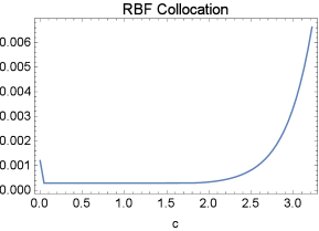
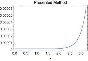
Figure 1: Graphs of maximum absolute error versus shape parameter with Gaussian RBF, $N=32$ and $\epsilon=\frac{1}{2^{5}}$, for Example 4.1.

For this example, the maximum absolute errors are presented in Table 1 for various values of $N$ and $\epsilon$ and they are compared with the best reported results in [36] and RBF collocation method. The Gaussian RBF with $c=\frac{18}{100}$ is used for presented method and RBF collocation method. Graphs of maximum absolute error versus shape parameter with Gaussian RBF, $N=32$ and $\epsilon=\frac{1}{2^{5}}$ are given in Figure 1. The reported results show that more accurate approximate solutions can be obtained using more mesh points. The numerical simulations show that the presented method is robust and accurate and remains stable as shape parameter gets smaller in contrast with the existing radial basis functions methods.

Example 4.2

Consider the Poisson’s equation,

$$-\Delta u=-\left(\frac{\partial^{2}u}{\partial x^{2}}+\frac{\partial^{2}u}{\partial y^{2}}\right)=f(x,y),\hskip 14.22636pt(x,y)\in[0,1]\times[0,1]$$

with the Robin boundary conditions

$$\begin{array}[]{ll}u|_{x=0}=0,\hskip 14.22636ptu|_{y=0}=0,\\ u_{v}|{x=1}=g_{N},\\ (u_{v}+\alpha u)|_{y=1}=g_{R},\\ \end{array}$$

where $\alpha>0$,(e.g.,$\alpha=2$) and $v$ is the outward normal vector to the boundary. The functions $f,g_{N}$ and $g_{R}$ are given such that the exact solution is [37],

$$u=\sin(\frac{\pi x}{6})\sin(\frac{7\pi x}{4})\sin(\frac{3\pi y}{4})\sin(\frac{5\pi y}{4}).$$

N	$7\times 7$	$9\times 9$	$11\times 11$	$13\times 13$
[37]	9.30e-3	5.92e-5	4.32e-6	1.10e-6
RBF collocation	3.31818e-3	3.03747e-4	6.31077e-6	1.06431e-7
Presented method	2.64223e-4	1.42617e-5	2.11003e-7	1.0773e-8

Table 2: Maximum absolute errors, comparison of results for Example 4.2.

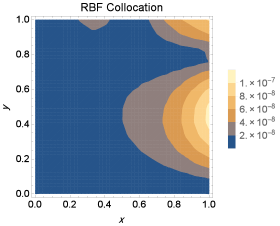
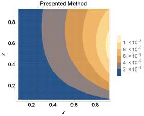
Figure 2: Distribution of the absolute error with Gaussian RBF, $N=13\times 13$ and $c=1$, for Example 4.2.

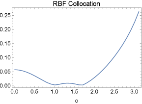
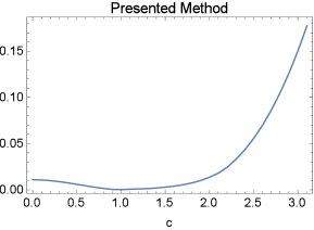
Figure 3: Graphs of maximum absolute error versus shape parameter with Gaussian RBF and $N=7\times 7$, for Example 4.2.

The maximum absolute errors are presented in Table 2 for various values of $N$ and they are compared with the reported results in [37] and RBF collocation method. The Gaussian RBF with $c=1$ is used for presented method and RBF collocation method. Figure 2 shows the distribution of the absolute error of presented method and RBF collocation method with Gaussian RBF, $N=13\times 13$ and $c=1$. The reported results show that more accurate approximate solutions can be obtained using more mesh points. Comparison of numerical results show that the presented method has the exponential convergence rates and is more accurate than RBF collocation method and combination of RBF collocation and Ritz–Galerkin method [37]. Graphs of maximum absolute error versus shape parameter with Gaussian RBF, $N=7\times 7$ are given in Figure 3 which show that remain stable as shape parameter gets smaller in contrast with the existing radial basis functions methods.

Example 4.3

Consider the Poisson’s equation [38],

$$\Delta u=y(1-y)\sin^{3}x,\hskip 14.22636pt(x,y)\in[0,\pi]\times[0,1]$$

with the homogeneous Dirichlet boundary conditions

$$u(x,0)=u(x,1)=u(0,y)=u(\pi,y)=0.$$

The exact solution is given by

$$\begin{array}[]{ll}u(x,y)&=\frac{3e^{-y}\left(-2e-2e^{2y}+e^{y}(1+e)(2+(-1+y)y)\right)\sin(x)}{4(1+e)}\\ &+\frac{3e^{-3y}\left(2e^{3}+2e^{6y}-e^{3y}(1+e^{3})(2+9(-1+y)y)\right)\sin(3x)}{324(1+e^{3})}.\\ \end{array}$$

N	$\rho_{K}$[38]	$\rho_{H}$[38]	$\rho_{RBFC}$	$\rho_{1}$	$\rho_{2}$
$8\times 4$	1.103747e-2	1.062891e-2	7.4357e-2	2.1191e-3	2.84849e-3
$10\times 6$	2.739293e-3	3.451799e-3	1.58122e-3	3.60844e-5	3.10566e-4
$16\times 8$	2.707006e-4	2.082886e-4	1.92361e-5	5.17671e-7	1.59593e-7
$20\times 12$	3.894511e-5	1.273363e-5	3.60382e-9	8.72329e-11	6.0899e-11

Table 3: Relative errors, comparison of results for Example 4.3.

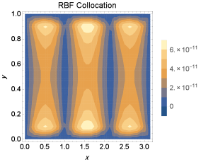
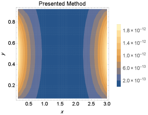
Figure 4: Distribution of the absolute error with Gaussian RBF, $N=20\times 12$ and $c=0.3041$ for RBF collocation and $c=0.01$ for Presented method, for Example 4.3.

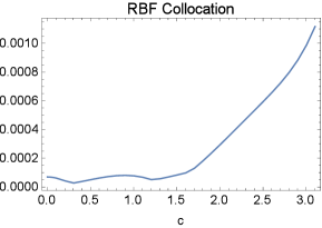
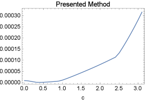
Figure 5: Graphs of maximum absolute error versus shape parameter with Gaussian RBF, $N=10\times 6$, for Example 4.3.

The relative errors are presented in Table 3 for various values of $N$ and they are compared with the best reported results in [38] contain Kansa’s and Hermit based RBF method and RBF collocation method. $\rho_{RBFC}$ is relative error of RBF collocation method with Gaussian RBF with $c=0.3041$ and $\rho_{1}$ and $\rho_{2}$ are relative errors of presented method with Gaussian RBF with $c=0.4041$ and $c=0.01$, respectively. $\rho_{K}$ and $\rho_{H}$ are reported relative errors in [38] with optimal shape parameters for Kansa’s and Hermit based RBF method, respectively. Figure 4 shows the distribution of the absolute error of presented method and RBF collocation method with Gaussian RBF, $N=20\times 12$ with $c=0.3041$ for RBF collocation and $c=0.01$ for Presented method. The reported results show that more accurate approximate solutions can be obtained using more mesh points. Comparison of numerical results show that the presented method is more accurate than the existing RBF methods. Graphs of maximum absolute error versus shape parameter with Gaussian RBF, $N=10\times 6$ are given in Figure 5 which show that remain stable as shape parameter gets smaller in contrast with the collocation radial basis functions methods.

Example 4.4

Consider the Poisson’s equation [39],

$$\Delta u=2e^{x-y},\hskip 14.22636pt(x,y)\in[0,1]\times[0,1]$$

with the nonhomogeneous Dirichlet boundary conditions

$$\begin{array}[]{lll}u(0,y)&=g_{1}(y),\hskip 14.22636ptu(1,y)&=g_{2}(y),\\ u(x,0)&=h_{1}(x),\hskip 14.22636ptu(x,1)&=h_{2}(x).\\ \end{array}$$

The exact solution is given by

$$u(x,y)=e^{x-y}+e^{x}\cos y.$$

N	$5\times 5$	$10\times 10$	$15\times 15$	$20\times 20$
RBF collocation	1.56591e-4	3.89263e-11	8.55909e-19	4.57185e-27
Presented method	8.12108e-9	4.6856e-15	3.36241e-23	1.92864e-32

Table 4: Maximum absolute errors, comparison of results for Example 4.4.

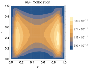
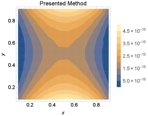
Figure 6: Distribution of the absolute error with Gaussian RBF, $N=10\times 10$ and $c=0.01$, for Example 4.4.

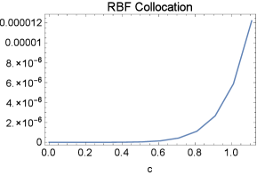
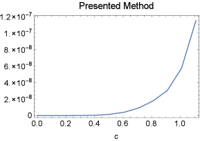
Figure 7: Graphs of maximum absolute error versus shape parameter with Gaussian RBF, $N=10\times 10$, for Example 4.4.

The Maximum absolute errors are presented in Table 4 for various values of $N$. For comparison, the best result reported in [39] has $1.28\times 10^{-4}$ maximum absolute error with $81$ collocation points and $c=1.2$ shape parameter. Figure 6 shows the distribution of the absolute error of presented method and RBF collocation method with Gaussian RBF, $N=10\times 10$ with $c=0.01$ for RBF collocation and Presented method. The reported results show that more accurate approximate solutions can be obtained using more mesh points. Comparison of numerical results show that the presented method is more accurate than the existing RBF methods. Graphs of maximum absolute error versus shape parameter with Gaussian RBF, $N=10\times 10$ are given in Figure 7, which show that the presented method is more accurate than RBF collocation method for various shape parameters.

Example 4.5

Consider the Poisson’s equation [38],

$$\Delta u=\sin x-\sin^{3}x,\hskip 14.22636pt(x,y)\in[0,\frac{\pi}{2}]\times[0,2],$$

with the Dirichlet and Neumann boundary conditions

$$u(0,y)=u_{x}(\frac{\pi}{2},y)=u_{y}(x,0)=u_{y}(x,2)=0.$$

The exact solution is given by

$$u(x,y)=-\frac{1}{4}\sin(x)-\frac{1}{36}\sin(3x).$$

N	$\rho_{K}$[38]	$\rho_{H}$[38]	$\rho_{RBFC}$	$\rho_{1}$	$\rho_{2}$
$5\times 5$	2.181029e-2	4.327029e-2	1.56966e-2	1.2886e-3	2.31536e-2
$7\times 7$	6.910084e-3	1.871798e-4	7.45327e-3	1.34064e-5	1.33894e-3
$10\times 10$	9.265197e-5	5.126676e-5	5.75242e-4	3.29045e-8	5.32917e-6
$14\times 14$	1.138751e-5	1.725526e-6	5.59595e-5	4.62586e-11	1.74509e-9
$20\times 20$	5.501057e-6	6.217559e-7	1.34064e-6	8.15272e-17	1.42493e-15

Table 5: Relative errors, comparison of results for Example 4.5 and $c=0.4641,0.01$ for presented method and $c=0.5641$ RBF collocation..

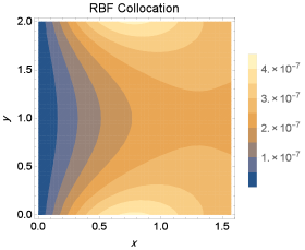
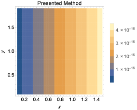
Figure 8: Distribution of the absolute error with Gaussian RBF, $N=20\times 20$ and $c=0.5641$ for RBF collocation and $c=0.01$ for Presented method, for Example 4.5.

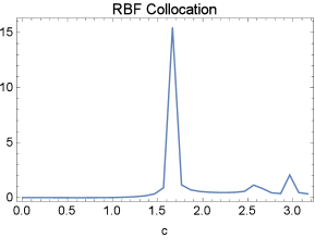
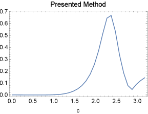
Figure 9: Graphs of maximum absolute error versus shape parameter with Gaussian RBF, $N=7\times 7$, for Example 4.5.

For this example, the relative errors are presented in Table 5 for various values of $N$ and they are compared with the best reported results in [38] contain Kansa’s and Hermit based RBF method and RBF collocation method. $\rho_{RBFC}$ is relative error of RBF collocation method with Gaussian RBF with $c=0.5641$ and $\rho_{1}$ and $\rho_{2}$ are relative errors of presented method with Gaussian RBF with $c=0.4641$ and $c=0.01$, respectively. $\rho_{K}$ and $\rho_{H}$ are reported relative errors in [38] with optimal shape parameters for Kansa’s and Hermit based RBF method, respectively. Figure 8 shows the distribution of the absolute error of presented method and RBF collocation method with Gaussian RBF, $N=20\times 20$ with $c=0.5641$ for RBF collocation and $c=0.01$ for Presented method. The reported results show that more accurate approximate solutions can be obtained using more mesh points. Comparison of numerical results show that the presented method is more accurate than the existing RBF methods. Graphs of maximum absolute error versus shape parameter with Gaussian RBF, $N=7\times 7$ are given in Figure 9.

Example 4.6

Consider the nonlocal multi–point Poisson’s equation [40],

$$\Delta u=f,\hskip 14.22636pt(x,y)\in[0,1]\times[0,2],$$

with the multi–point boundary conditions

$$\begin{array}[]{llll}u(0,y)&=u(1,y)=0,\\ u(x,2)&=g(x),\\ u(x,0)&=\frac{1}{4}u(x,\frac{3}{5})+\frac{1}{2}u(x,\frac{6}{5})+\frac{1}{4}u(x,\frac{9}{5}).\\ \end{array}$$

The functions $f$ and $g$ are given such that the exact solution is,

$$u(x,y)=\frac{1}{500}\left((e^{\pi x}-1)(e^{\pi x}-e^{\pi})\sin(\frac{5\pi}{6}y)+e^{\pi y(\frac{3}{5}-y)(\frac{6}{5}-y)(\frac{9}{5}-y)}\sin(\pi x)\right).$$

N	$5\times 10$	$8\times 16$	$10\times 20$	$12\times 24$
RBF collocation	4.09711e-2	1.70686e-3	9.94226e-5	4.15599e-6
Presented method	5.47254e-3	1.09398e-4	1.44713e-5	2.80392e-6

Table 6: Maximum absolute errors, comparison of results for Example 4.6.

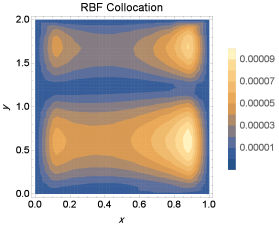
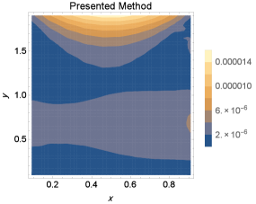
Figure 10: Distribution of the absolute error with Gaussian RBF, $N=10\times 20$ and $c=0.01$, for Example 4.6.

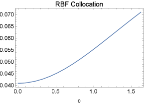
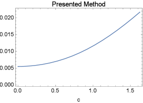
Figure 11: Graphs of maximum absolute error versus shape parameter with Gaussian RBF, $N=5\times 10$, for Example 4.6.

The maximum absolute errors are presented in Table 6 for various values of $N$ and they are compared with the RBF collocation method. The Gaussian RBF with $c=0.01$ is used for presented method and RBF collocation method. Figure 10 shows the distribution of the absolute error of presented method and RBF collocation method with Gaussian RBF, $N=10\times 20$ and $c=0.01$. The reported results show that more accurate approximate solutions can be obtained using more mesh points. Comparison of numerical results show that the presented method is more accurate than the RBF collocation method. Graphs of maximum absolute error versus shape parameter with Gaussian RBF, $N=5\times 10$ are given in Figure 11.

Example 4.7

Consider the Poisson’s equation [41],

$$\Delta u(x,y,z)=\frac{6}{(4+x+y+z)^{3}},\hskip 14.22636pt(x,y,z)\in\Omega=[-\frac{1}{2},\frac{1}{2}]^{3},$$

with the Dirichlet boundary conditions

$$u=g(\textbf{x}),\hskip 14.22636pt\textbf{x}\in\Gamma,$$

where $\Gamma$ is the boundary of $\Omega$ and $g$ is given such that the exact solution is,

$$u(x,y,z)=\frac{1}{(4+x+y+z)}.$$

N	$4\times 4\times 4$	$5\times 5\times 5$	$6\times 6\times 6$	$7\times 7\times 7$
RBF collocation	3.8223e-5	4.86452e-6	6.73616e-7	8.47629e-8
Presented method	1.02919e-7	1.49101e-8	2.4369e-9	3.43708e-10

Table 7: Maximum absolute errors, comparison of results for Example 4.7 with $N=7\times 7\times 7$ and $c=0.01$.

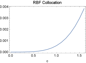
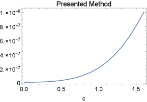
Figure 12: Graphs of maximum absolute error versus shape parameter with Gaussian RBF, $N=5\times 5\times 5$, for Example 4.7.

The maximum absolute errors are presented in Table 7 for various values of $N$ and they are compared with the RBF collocation method. The Gaussian RBF with $c=0.01$ is used for presented method and RBF collocation method. For comparison, the best result reported in [41] has $10^{-5}$ maximum absolute error with $7\times 7\times 7$ points. The reported results show that more accurate approximate solutions can be obtained using more mesh points. Graphs of maximum absolute error versus shape parameter with Gaussian RBF, $N=5\times 5\times 5$ are given in Figure 12, which show that the presented method is more accurate than RBF collocation method for various shape parameters.

5 Conclusions

In this paper, we introduce a new approach for the imposing various boundary conditions on radial basis functions and their application in pseudospectral radial basis function method. The various boundary conditions such as Dirichlet, Neumann, Robin, mixed and multi–point boundary conditions for one, two and three-dimensional problems, have been considered. Here we propose a new technique to force the radial basis functions to satisfy the boundary conditions exactly. Some new kernels are constructed using general kernels in a manner which satisfies required conditions and we prove that if the reference kernel is positive definite then the newly constructed kernel is positive definite, also. Furthermore, we show that the collocation matrix is nonsingular if some conditions are satisfied. It can improve the applications of existing methods based on radial basis functions especially the pseudospectral radial basis function method to handling the differential equations with more complicated boundary conditions. Several examples with various boundary conditions have been considered for validation of the proposed technique and the results are compared with the RBF collocation method and the best-reported results in the literature.

References

- [1] S. Abbasbandy, H. Roohani Ghehsareh, I. Hashim, A. Alsaedi, A comparison study of meshfree techniques for solving the two-dimensional linear hyperbolic telegraph equation, Engineering Analysis with Boundary Elements 47 (2014), 10–20.
- [2] S. Abbasbandy, H. Roohani Ghehsareh, I. Hashim, Numerical analysis of a mathematical model for capillary formation in tumor angiogenesis using a meshfree method based on the radial basis function, Engineering Analysis with Boundary Elements 36(12) (2012), 1811–1818.
- [3] S. Abbasbandy, H. Roohani Ghehsareh, I. Hashim, A meshfree method for the solution of two-dimensional cubic nonlinear Schrödinger equation, Engineering Analysis with Boundary Elements 37(6) (2013), 885–898.
- [4] K. Parand, S. Abbasbandy, S. Kazem, A. R. Rezaei, Comparison between two common collocation approaches based on radial basis functions for the case of heat transfer equations arising in porous medium, Communications in Nonlinear Science and Numerical Simulation 16(3) (2011), 1396-1407.
- [5] E. J. Kansa, R. C. Aldredge, L. Ling, Numerical simulation of two-dimensional combustion using mesh-free methods, Engineering analysis with boundary elements 33(7) (2009), 940-950.
- [6] E. Shivanian, A new spectral meshless radial point interpolation (SMRPI) method: A well-behaved alternative to the meshless weak forms, Engineering Analysis with Boundary Elements 54 (2015), 1–12.
- [7] E. Shivanian, Analysis of meshless local and spectral meshless radial point interpolation (MLRPI and SMRPI) on 3-D nonlinear wave equations, Ocean Engineering 89 (2014), 173–188.
- [8] H. R. Ghehsareh,S. H. Bateni, A. Zaghian, A meshfree method based on the radial basis functions for solution of two-dimensional fractional evolution equation, Engineering Analysis with Boundary Elements 61 (2015), 52–60.
- [9] S. Kazem, J. A. Rad and K. Parand, Radial basis functions methods for solving Fokker Planck equation, Engineering Analysis with Boundary Elements 36(2) (2012), 181–189.
- [10] J. A. Rad, K. Parand and S. Abbasbandy, Local weak form meshless techniques based on the radial point interpolation (RPI) method and local boundary integral equation (LBIE) method to evaluate European and American options, Communications in Nonlinear Science and Numerical Simulation 22(1) (2015), 1178–1200.
- [11] S. Abbasbandy, B. Azarnavid and M. S. Alhuthali, A shooting reproducing kernel Hilbert space method for multiple solutions of nonlinear boundary value problems, Journal of Computational and Applied Mathematics, 279 (2015): 293–305.
- [12] B. Azarnavid and K. Parand, An iterative reproducing kernel method in Hilbert space for the multi–point boundary value problems, Journal of Computational and Applied Mathematics, 328 (2018): 151–163.
- [13] S. Abbasbandy, B. Azarnavid, Some error estimates for the reproducing kernel Hilbert spaces method, Journal of Computational and Applied Mathematics, 296 (2016): 789–797.
- [14] B. Azarnavid, F. Parvaneh and S. Abbasbandy, Picard-Reproducing Kernel Hilbert Space Method for Solving Generalized Singular Nonlinear Lane-Emden Type Equations, Mathematical Modelling and Analysis, 20(6) (2015): 754–767.
- [15] B. Azarnavid, E. Shivanian, K. Parand and Soudabeh Nikmanesh, Multiplicity results by shooting reproducing kernel Hilbert space method for the catalytic reaction in a flat particle, Journal of Theoretical and Computational Chemistry 17(02) (2018): 1850020.
- [16] B. Azarnavid, K. Parand and S. Abbasbandy, An iterative kernel based method for fourth order nonlinear equation with nonlinear boundary condition, Communications in Nonlinear Science and Numerical Simulation, 59 (2018): 544–552.
- [17] M. Emamjome, B. Azarnavid and H. Roohani Ghehsareh, A reproducing kernel Hilbert space pseudospectral method for numerical investigation of a two-dimensional capillary formation model in tumor angiogenesis problem, Neural Computing and Applications, (2017): 1–9.
- [18] O. A. Arqub, Fitted reproducing kernel Hilbert space method for the solutions of some certain classes of time-fractional partial differential equations subject to initial and Neumann boundary conditions, Computers & Mathematics with Applications, 73(6) (2017): 1243–1261.
- [19] M. Al-Smadi, O. A. Arqub, N. Shawagfeh and S. Momani, Numerical investigations for systems of second-order periodic boundary value problems using reproducing kernel method, Applied Mathematics and Computation, 291 (2016): 137–148.
- [20] O. A. Arqub, Approximate solutions of DASs with nonclassical boundary conditions using novel reproducing kernel algorithm, Fundamenta Informaticae, 146(3) (2016): 231–254.
- [21] O. A. Arqub, The reproducing kernel algorithm for handling differential algebraic systems of ordinary differential equations, Mathematical Methods in the Applied Sciences, 39(15) (2016): 4549–4562.
- [22] A. Akgül and D. Baleanu, On solutions of variable-order fractional differential equations, An International Journal of Optimization and Control: Theories & Applications (IJOCTA), 7(1) (2017): 112–116.
- [23] M. G. Sakar, A. Akgül and D. Baleanu, On solutions of fractional Riccati differential equations, Advances in Difference Equations, 2017(1) (2017): 39.
- [24] J. Amani Rad, Jamal K. Parand, Pricing American options under jump-diffusion models using local weak form meshless techniques, International Journal of Computer Mathematics (2016), 1–25.
- [25] G. E. Fasshauer, RBF collocation methods as pseudospectral methods, WIT transactions on modelling and simulation 39 (2005).
- [26] S. A. Sarra, Adaptive radial basis function methods for time dependent partial differential equations, Applied Numerical Mathematics 54(1) (2005), 79–94.
- [27] A. J. M. Ferreira, G. E. Fasshauer, An RBF-Pseudospectral approach for the static and vibration analysis of composite plates using a higher-order theory, International journal for computational methods in engineering science and mechanics 8(5) (2007), 323–339.
- [28] M. Uddin, Marjan, RBF-PS scheme for solving the equal width equation, Applied Mathematics and Computation 222 (2013), 619–631.
- [29] G. E. Fasshauer, J. G. Zhang, On choosing optimal shape parameters for RBF approximation, Numerical Algorithms 45 (2007), 345- 368.
- [30] A. J. M. Ferreira, G. E. Fasshauer, Computation of natural frequencies of shear deformable beams and plates by an RBF-pseudospectral method, Computer Methods in Applied Mechanics and Engineering 196(1) (2006), 134–146.
- [31] M. Uddin and S. Ali, RBF-PS method and fourier pseudospectral method for solving stiff nonlinear partial differential equations, Mathematical Sciences Letters 2(1) (2012) 55 -61.
- [32] M. Uddin and R.J. Ali, RBF-PS scheme for the numerical solution of the complex modified Korteweg de Vries equation, Applied Mathematics & Information Sciences Letters 1(1) (2012), 9–17.
- [33] E. Larsson and B. Fornberg, A numerical study of some radial basis function based solution methods for elliptic PDEs, Computers & Mathematics with Applications 46(5) (2003), 891–902.
- [34] H. Wendland. Scattered data approximation. Vol. 17. Cambridge university press, 2004.
- [35] N. Aronszajn, Theory of reproducing kernels, Transactions of the American mathematical society 68(3) (1950), 337–404.
- [36] A. R. Ansari and A. F. Hegarty, Numerical solution of a convection diffusion problem with Robin boundary conditions, Journal of computational and applied mathematics 156(1) (2003), 221–238.
- [37] H. H. Yun, Z.C. Li and A. H. D. Cheng, Radial basis collocation methods for elliptic boundary value problems, Computers & Mathematics with Applications 50(1) (2005), 289–320.
- [38] G. F. Fasshauer, Solving partial differential equations by collocation with radial basis functions, In Proceedings of Chamonix, vol. 1997, pp. 1–8. Vanderbilt University Press Nashville, TN, 1996.
- [39] C. S. Chen, Y. C. Hon and R. A. Schaback, Scientific computing with radial basis functions, Department of Mathematics, University of Southern Mississippi, Hattiesburg, MS 39406 (2005).
- [40] E. A. Volkov and A. A. Dosiyev, On the numerical solution of a multilevel nonlocal problem, Mediterranean Journal of Mathematics (2016), 1–16.
- [41] C. C. Tsai, Generalized polyharmonic multiquadrics, Engineering Analysis with Boundary Elements 50 (2015), 239–248.