Efficient Inter-Geodesic Distance Computation
and Fast Classical Scaling

Abstract

Multidimensional scaling (MDS) is a dimensionality reduction tool used for information analysis, data visualization and manifold learning. Most MDS procedures embed data points in low-dimensional Euclidean (flat) domains, such that distances between the points are as close as possible to given inter-point dissimilarities. We present an efficient solver for classical scaling, a specific MDS model, by extrapolating the information provided by distances measured from a subset of the points to the remainder. The computational and space complexities of the new MDS methods are thereby reduced from quadratic to quasi-linear in the number of data points. Incorporating both local and global information about the data allows us to construct a low-rank approximation of the inter-geodesic distances between the data points. As a by-product, the proposed method allows for efficient computation of geodesic distances.

1 Introduction

With the increasing availability of digital information, the need for data simplification and dimensionality reduction tools constantly grows. Self-Organizing Map (SOM) [19], Local Coordinate Coding [42, 43], Multidimensional Scaling (MDS), and Isomap [5, 39] are examples of data reduction techniques that are used to simplify data and hence reduce computational and space complexities of related procedures.

MDS embeds the data into a low-dimensional Euclidean (flat embedding) space, while attempting to preserve the distance between each pair of points. Flat embedding is a fundamental step in various applications in the fields of data mining, statistics, manifold learning, non-rigid shape analysis, and more. For example, in [24], Panozzo et al. demonstrated, using MDS, how to generalize Euclidean weighted averages to weighted averages on surfaces. Weighted averages on surfaces could then be used to efficiently compute splines on surfaces, solve re-meshing problems, and find shape correspondences. Zigelman et al. [44] used MDS for texture mapping, while Schwartz et al. [31, 14] utilized it to flatten models of monkeys’ cortical surfaces for further analysis. In [32, 29, 27], MDS was applied to image and video analysis. In [15] and [34], MDS was used to construct a bending invariant representation of surfaces, referred to as a canonical form. Such canonical forms reveal the intrinsic structure of the surface, and were used to simplify tasks such as non-rigid object matching and classification.

The bottleneck step in MDS is computing and storing all pairwise distances. For example, when dealing with geodesic distances computed on surfaces, this step is time-consuming and, in some cases, impractical. The fast marching method [18] is an example of one efficient procedure for approximating the geodesic distance map between all pairs of $p$ points on a surface. Its complexity is $O(p^{2}\log p)$ when used in a straightforward manner. Nevertheless, even when using such an efficient procedure, the complexities involved in computing and storing these distances are at least quadratic in the number of points.

One way to reduce these complexities is by considering only local distances between nearby data points. Attempts to do so were made, for example, in Locally Linear Embedding (LLE, [28]) Hessian Locally Linear Embedding (HLLE, [12]), and Laplacian eigenmaps [3]. For these methods, the effective time and space complexities are linear in the number of points. These savings, however, come at the expense of only capturing the local structure while the global geometry is ignored. In [36], De Silva and Tenenbaum suggested computing only distances between a small subset of landmarks. The landmarks were then embedded, ignoring the rest of the distances, and then the rest of the points were interpolated into the target flat space. The final embedding, however, was restricted to the initial one at the landmark points.

The Nyström method [2] is an efficient technique to reconstruct a positive semidefinite matrix using only a small subset of its columns and rows. Various recent techniques for approximating and reducing the complexities of MDS bear some resemblance to the Nyström method [26]. In [41] and [9], only a few columns of the pairwise distance matrix were computed, after which the Nyström method was used to interpolate the rest of the matrix. The main differences between these two methods are the column sampling schemes and the way to compute the initial geodesic distances. In the latter method, a regularization term was used for the pseudo-inverse in the Nyström method, which further improved the distance matrix reconstruction. [22] combined the Nyström method with Kernel-PCA [30] and demonstrated an efficient application of mesh segmentation. Recently, Spectral-MDS (SMDS) [1] obtained state-of-the-art results for efficiently approximating the embedding of MDS. There, geodesic distances are interpolated by exploiting a smoothness assumption through the Dirichlet energy. Complexities are reduced by translating the problem into the spectral domain and representing all inter-geodesic distances, considering only the first eigenvectors of the Laplace-Beltrami operator (LBO).

Here, we explore two methods, the Fast-MDS (FMDS) [33] and Nyström-MDS (NMDS) [35], for efficiently approximating inter-geodesic distances and, thereby, reduce the complexities of MDS. FMDS interpolates the distance map from a small subset of landmarks using a smoothness assumption as a prior, formulated through the bi-Laplacian operator [21, 6, 37]. As opposed to Spectral-MDS, the problem is solved in the spatial domain and no eigenvectors are omitted, so that accuracy is improved. Nevertheless, the time complexities remain the same. NMDS learns the distance interpolation coefficients from an initial set of computed distances. Both methods reconstruct the pairwise geodesic distance matrix as a low-rank product of small matrices and obtain a closed form approximation of classical scaling through small matrices.

Our numerical experiments compare FMDS and NMDS to all relevant methods mentioned above and demonstrate high efficiency and accuracy in approximating the embedding of MDS and the inter-geodesic distances. In practice, our methods embed $10K$-vertex shapes within less than a second, including all initializations, with an approximation error of $0.007\%$ from the same embedding obtained by MDS. When compared to exact geodesics [38] on surfaces, our methods approximate geodesic distances with a better average accuracy than fast marching, while computing $500$M geodesic distances per second.

The paper is organized as follows. In Section 2 we briefly review the classical scaling method. In Section 3 we develop two methods for geodesic distance interpolation from a few samples, formulated as a product of small-sized matrices. Section 4 discusses how to select the samples. In Section 5 we reformulate classical scaling through the small-sized matrices obtained by the interpolation. Section 6 provides support for the proposed methods by presenting experimental results and comparing to other methods. Finally, Section 7 discusses an extension of embedding on a sphere.

2 Classical Scaling

Given $p$ points $\{y_{i}\}_{i=1}^{p}$ equipped with some similarity measures $D_{ij}$ between them, multidimensional scaling (MDS) methods aim at finding an embedding $\{z_{i}\}_{i=1}^{p}$ in a low-dimensional Euclidean space $\mathbb{R}^{m}$ such that the Euclidean distances $\left\|{{z_{i}}-{z_{j}}}\right\|_{\mathbb{R}^{m}}$ are as close as possible to $D_{ij}$. When the points $\{y_{i}\}_{i=1}^{p}$ lie on a manifold, the affinities $D_{ij}$ can be defined as the geodesic distances between them. In this case, on which we focus in this paper, $D_{ij}$ are invariant to isometric deformations of the surface, thus revealing its intrinsic geometry. One way to define this problem, termed classical scaling, is through the minimization

$$\arg_{Z}\min{\left\|{Z{Z^{T}}+\frac{1}{2}JEJ}\right\|_{F}},$$ (1)

where $Z_{ij}=z_{i}^{j}$, ${E_{ij}}=D_{ij}^{2}$ and ${J_{ij}}={\delta_{ij}}-\frac{1}{p}$, and as usual, $\delta_{ij}=0$ for $i\neq j$ and $\delta_{ii}=1$ for all $i$. Denoting by $\tilde{V}\tilde{\Lambda}\tilde{V}^{T}$ the thin eigenvalue decomposition of the symmetric matrix $-\frac{1}{2}JEJ$, with only the $m$ largest eigenvalues and corresponding eigenvectors, the solution for this problem is given by $Z=\tilde{V}\tilde{\Lambda}^{\frac{1}{2}}$. This requires the computation of all pairwise distances in the $p\times p$ matrix $E$, which is not a practical solution method when dealing with more than a few thousand points. In this paper, we reconstruct $E$ from a small set of its columns. We formulate the reconstruction as a product of small-sized matrices, and show how to solve the above minimization problem without explicitly computing the reconstruction. Thus, we circumvent the bottleneck of classical scaling and significantly reduce both space and time complexities from quadratic to quasi-linear.

3 Distance Interpolation

Let $\cal{M}$ be a manifold embedded in some $\mathbb{R}^{k}$ space. Denote by $E(x,y)$ the squared geodesic distance between $x,y\in\cal{M}$. In the discrete domain $\cal{M}$ is represented by $p$ points, and $E$ is represented by a $p\times p$ matrix. In Sections 3.1 and 3.2 we develop two methods for reconstructing $E$ by decomposing it into smaller-sized matrices $E\approx STS^{T}$.

3.1 A smoothness-based reconstruction

One cornerstone of numerical algebra is representing a large matrix as a product of small-sized matrices [13, 23]. Compared to such classical decomposition, better approximations can be obtained when considering a specific data model. Here, we exploit the fact that the elements of the matrix to be reconstructed are squared geodesic distances, derived from some smooth manifold.

Starting from the continuous case, let $x_{0}\in\cal{M}$ be an arbitrary point on the manifold, and denote by $\bar{e}\colon x\in\cal{M}\to\mathbb{R}$ the squared geodesic distance from $x_{0}$ to all other points $x\in\cal{M}$. Assume the values of $\bar{e}(x)$ are known in a set of $n$ samples $\{x_{i}\}_{i=1}^{n}\in\cal{M}$, and denote these values by $\{r_{i}\}_{i=1}^{n}$. We expect the distance function $\bar{e}(x)$ to be smooth on the manifold, as nearby points should have similar $\bar{e}(x)$ values. Therefore, we aim to find a function $\bar{e}(x)$ that both is smooth and satisfies the constraints $\bar{e}(x_{i})=r_{i}$. This can be formulated through the minimization

$$\arg_{\bar{e}}\min{\mathcal{E}(\bar{e})}\hskip 14.22636pt\mbox{s.t.}\hskip 14.22636pt\bar{e}(x_{i})=r_{i},$$ (2)

where the energy $\mathcal{E}(\bar{e})$ is some smoothness measure of $\bar{e}(x)$ on $\cal{M}$. One possible, somewhat sensitive, choice of $\mathcal{E}(\bar{e})$ is the Dirichlet energy

$$\mathcal{E}(\bar{e})=\int\limits_{x\in\cal{M}}{\|\nabla\bar{e}(x)\|^{2}_{2}da(x)},$$ (3)

used in [1], where $da(x)$ is the infinitesimal volume element and the gradient is computed with respect to the manifold. The Dirichlet energy with point constraints could lead to removable discontinuities; see Figure 1. Therefore, instead, we use a different popular measure that yields a decomposition that is both simple and less sensitive. Denoting by $\bar{l}(x)=\Delta\bar{e}(x)$ the result of the LBO on $\cal{M}$ applied to $\bar{e}$, this energy is defined as

$$\mathcal{E}(\bar{e})=\int\limits_{x\in\cal{M}}{{{\left(\Delta\bar{e}(x)\right)}^{2}}da(x)}=\int\limits_{x\in\cal{M}}{{{\left({\bar{l}(x)}\right)}^{2}}da(x)}.$$ (4)

It yields the bi-Laplacian as the main operator in the resulting Euler-Largange equation [21, 6, 37].

In the discrete case, we define the diagonal matrix $A$ such that its diagonal is a discretization of $da(x)$ about each corresponding vertex, and denote by the vectors $l$ and $e$ the discretization of $\bar{l}$ and $\bar{e}$, respectively. Note that $e$ is a column in the matrix $E$, which was defined earlier as the pairwise squared geodesics. Denote by $L$ the discretization of the LBO, such that $l=Le$. We use the cotangent-weight Laplacian with Dirichlet boundary conditions in our experiments [25], [3]. Any discretization matrix of the LBO, however, can be used. Following these notations, the energy now reads

$$\mathcal{E}(e)=\sum\limits_{i=1}^{p}{{l_{i}}^{2}{A_{ii}}}={l^{T}}Al={e^{T}}{L^{T}}ALe,$$ (5)

and the interpolation becomes

$$e^{*}=\arg_{e}\min{e^{T}}{L^{T}}ALe\hskip 14.22636pt\mbox{s.t.}\hskip 14.22636ptBe=r,$$ (6)

where $r$ is an $n\times 1$ vector holding the values $\{r_{i}\}_{i=1}^{n}$. Recall that $r$ is a subset of $e$. Hence, the $n\times p$ matrix $B$ can easily be defined such that $Be=r$. Since the constraints may be contaminated with noise, a relaxed form of the problem using a penalty function is used instead. This can be formulated as

$$e^{*}=\mathop{\arg_{e}\min}({e^{T}}{L^{T}}ALe+\mu{\left\|{Be-r}\right\|^{2}}),$$ (7)

where $\mu$ is a sufficiently large scalar. This is a quadratic equation and its solution is given by

$$M = {({L^{T}}AL+\mu{B^{T}}B)^{-1}}\mu{B^{T}}$$ (8)

$$e^{*} = Mr.$$ (9)

To sum up, given a set of samples $r$ of the distance function $e$, $Mr$ is a reconstruction of $e$ in the sense of being a smooth interpolation from its samples. Figures 1 and 2 demonstrate the reconstruction of $e$ from its samples for flat and curved manifolds. Recall that $e$ is the squared geodesic distance from a point $x_{0}$ to the rest of the points on the manifold. In this example, we chose $x_{0}$ at the center of the manifold $\cal{M}$. In Figure 1, the surface is flat and hence the function $e$ is simply the squared Euclidean distance from a point in $\mathbb{R}^{2}$, $z=x^{2}+y^{2}$, where $x$ and $y$ are the Euclidean coordinates. We compare the suggested energy to the Dirichlet energy. As can be seen, when using the Dirichlet energy, the function includes sharp discontinuities at the constraint points.

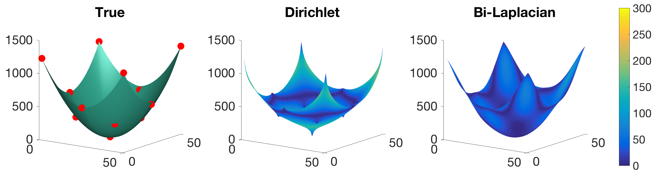
Figure 1: Reconstruction of $e$ (a column of $E$) on a flat surface. Left: The true values of $e$. The chosen $n=13$ samples are marked by red points. Middle and right: The reconstructed function $e^{*}=Mr$ using the Dirichlet and Laplacian energies. For comparison, we colored the function according to the absolute error $|e^{*}-e|$.

Figure 2: Reconstruction of $e$ (a column of $E$) on a curved surface. Left: The curved surface. Middle: The true values of the distance function $e$, measured from the middle point of the surface, and sampled at $n=30$ red points. Right: The reconstructed function $e^{*}=Mr$ using the suggested energy.

In Equation (7), a larger value of $\mu$ corresponds to stronger constraints, in the sense that the surface is restricted to pass closer to the constraints. In the next experiment, we measure the average reconstruction error $\frac{\|e^{*}-e\|_{2}}{\|e\|_{2}}$, with respect to the parameter $\mu$, for a random set of geodesic paths $\{e\}$ on the hand and giraffe shapes from the SHREC dataset. It can be seen that larger values of $\mu$ lead to better approximations up to a limit that depends on the number of samples. This saturation occurs at a point where the surface approaches the constraints up to a negligible distance with respect to its reconstruction error at the remaining points. Very large values of $\mu$ might lead to numerical errors in the inversion step of Equation (8). In practice, as a typical number of samples in our method is $20$–$100$, any value between $10^{4}$ and $10^{10}$ would be a good choice of $\mu$.

Figure 3: Average reconstruction error w.r.t. the penalty parameter $\mu$.

Next, since $e$ is a column in the matrix $E$, we reconstruct all the other columns in the same manner. Notice that the matrix $M$ does not depend on the values of $e$, but only on the samples’ locations. Hence, it can be computed once and used to reconstruct all columns. Moreover, it is possible to formulate the reconstruction of all the columns of $E$ simultaneously using a simple matrix product. Let us choose $n\ll p$ columns of $E$ and let the $p\times n$ matrix $R$ hold these columns. The locations of the columns in $E$ correspond to the locations of the samples in the manifold. Each column of $R^{T}$ corresponds to a vector $r$, which contains the distances from the $n$ samples to a point $x_{0}$, which corresponds to the column. The column selection and the computation of $R$ are discussed in Section 4. Now, all columns of $E$ can be interpolated simultaneously by the product

$$\hat{E}=MR^{T}.$$ (10)

Since $E$ is symmetric by definition, we symmetrize its reconstruction by

$$\hat{E}=\frac{1}{2}(MR^{T}+RM^{T}).$$ (11)

Notice that $\hat{E}$ is a low-rank reconstruction of $E$ with a maximal rank of $2n$, because $R$ is of size $p\times n$, which means the rank of $MR^{T}$ is at most $n$. Therefore, the rank of $\hat{E}=\frac{1}{2}(MR^{T}+RM^{T})$ is at most $2n$. Consequently, $\hat{E}$ can be written as a product of matrices that are no larger than $2n\times p$. These matrices can be obtained as follows. Denote by ${S=(M|R)}$ the horizontal concatenation of $M$ and $R$, and define the block matrix $T=\frac{1}{2}\left({\begin{array}[]{*{20}{c}}{{0_{n\times n}}}&{{I_{n\times n}}}\\ {{I_{n\times n}}}&{{0_{n\times n}}}\end{array}}\right)$, where $I$ is the identity matrix. It can be verified that

$$\hat{E}=\frac{1}{2}(MR^{T}+RM^{T})=ST{S^{T}}.$$ (12)

We actually only need to keep the matrices $S$ and $T$ instead of the whole matrix $\hat{E}$, which reduces the space complexity from $O(p^{2})$ to $O(np)$. In our experiments, between $20$ and $100$ samples were enough for accurate reconstruction of $E$, where the number of vertices $p$ was in the range of $10^{3}$ to $10^{6}$.

Above we derived a low-rank approximation of the matrix $E$ from a set of known columns. The same interpolation ideas can be used for other tasks such as geodesics extrapolation [8] and matrix completion [16], in which a matrix is reconstructed from a set of known entries and the columns may vary in their structure.

3.2 A learning-based reconstruction

In Section 3.1, we derived a reconstruction $\hat{E}=STS^{T}$ by exploiting the smoothness assumption of the distances on the manifold. Although the suggested energy minimization results in a simple low-rank reconstruction of $E$, this might not be the best way to interpolate the distances. We now formulate a different decomposition based on a learning approach.

As before, we choose $n$ arbitrary columns of $E$ and let $R$ hold these columns. In Section 3.1, we constructed an interpolation matrix $M$ using the LBO as a smoothness measure such that $E\approx MR^{T}$ or similarly $E\approx RM^{T}$. Here we attempt to answer the following question: Is it possible to construct a matrix $M$ that would yield a better reconstruction? The matrix $M$ for the best reconstruction of $E$ in terms of the Frobenius norm is obtained by

$$\arg_{M}\min\|RM^{T}-E\|_{F}^{2},$$ (13)

and the solution is given by $M^{T}=R^{+}E$. In this case, the reconstruction is nothing but a projection of $E$ onto the subspace spanned by the columns of $R$,

$$\hat{E}=RR^{+}E.$$ (14)

We cannot, however, compute the best $M$ since we do not know the entire matrix $E$. Hence, we suggest learning the coefficients of $M$ from the part of $E$ that we do know. This can be formulated using a Hadamard product as

$$\arg_{M}\min\|H\circ(RM^{T}-E)\|_{F}^{2},$$ (15)

where $H$ is a mask of the location of $R^{T}$ in $E$ (the known rows of $E$). The known rows of $E$ can be thought of as our training data for learning $M$. This has some resemblance to various matrix completion formulations, such as the Euclidean Distance Matrix (EDM) completion in [16]. Nevertheless, unlike previous methods, our primary goal here is to derive a formulation that can be expressed as a low-rank matrix product, preferably in a closed form, which is also efficient to compute. Next, define $R_{s}$ as the intersection of $R$ and $R^{T}$—that is, the elements that belong both to $R$ and $R^{T}$; see Figure 4(a).

The above equation is equivalent to

$$\arg_{M}\min\|R_{s}M^{T}-R^{T}\|_{F}^{2}.$$ (16)

In this form, the number of coefficients in $M$ is large with respect to our training data, which will result in overfitting. For instance, for a typical $R_{s}$ with independent columns, the reconstruction of the training data $R^{T}$ is perfect. Therefore, to avoid overfitting to the training data, we regularize this equation by reducing the number of learned coefficients. Let $C$ hold a subset of $n_{1}\leq n$ columns of $R$, and define $C_{s}$ as the intersection of $C$ and $R^{T}$; see Figure 4(b).

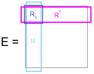
(a)

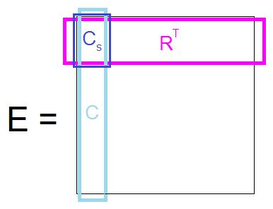
(b)

Figure 4: Demonstration of the partition of $E$, assuming the columns were chosen as the first ones. $R_{s}$ and $C_{s}$ are a part of the matrices $R$ and $C$. Note that $C$ and $C_{s}$ are subsets of $R$ and $R_{s}$.

The regularized formulation is

$$\arg_{M}\min\|C_{s}M^{T}-R^{T}\|_{F}^{2},$$ (17)

where $M$ is now a smaller matrix of size $p\times n_{1}$, and the solution is given by

$$M=(C_{s}^{T}C_{s})^{-1}C_{s}^{T}R^{T}=UR^{T},$$ (18)

yielding what is known as a CUR decomposition of $E$,

$$\hat{E}=CUR^{T}.$$ (19)

CUR decompositions are widely used and studied; see, for example, [13, 23]. Notice that when $n_{1}=n$, we obtain

$$\hat{E}=RR_{s}^{+}R^{T},$$ (20)

which is known as the Nyström decomposition for positive semidefinite matrices [2]. Choosing a large value for $n_{1}$ would result in overfitting to the training data. Alternatively, a low value would limit the rank of the approximated matrix and hence the ability to capture the data.

In Figure 5 (CUR) we demonstrate the reconstruction error of $E$ with respect to $n_{1}$, where $n=200$. There is a significant potential improvement compared to the previous un-regularized case of $n_{1}=n$, which results in the Nyström method.

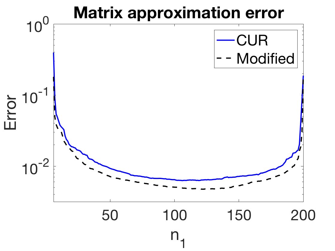
Figure 5: The reconstruction error with respect to $n_{1}$, given by $\frac{\|\hat{E}-E\|_{F}}{\|E\|_{F}}$, using the learning approach (CUR) and its proposed modification. $E$ is computed from the giraffe shape in the SHREC database (see experimental results).

In order to further reduce overfitting, we defined the matrix $C$ as a subset of the matrix $R$. A different choice of $C$ can lead to a better reconstruction of $E$. Denote by $V\Lambda V^{T}$ the eigenvalue decomposition of $R_{s}$ and denote by $\tilde{V}\tilde{\Lambda}\tilde{V}^{T}$ the thin eigenvalue decomposition of $R_{s}$ with only the $n_{1}$ eigenvalues with the largest magnitude and $n_{1}$ corresponding eigenvectors. The choice of

$$C=R\tilde{V}$$ (21)

formulates $C$ as a linear combination of the columns of $R$ instead of a subset of $R$, thus exploiting better learning of the data. Moreover, this will result in a symmetric decomposition of $E$. We have

$$C_{s} = R_{s}\tilde{V}$$ (22)

$$= V\Lambda V^{T}\tilde{V}$$ (23)

$$= V\Lambda V^{T}VI_{n\times n_{1}}$$ (24)

$$= V\Lambda I_{n\times n_{1}}$$ (25)

$$= \tilde{V}\tilde{\Lambda},$$ (26)

where $I_{n\times n_{1}}$ is the rectangular identity matrix (with ones along the main diagonal and zeros elsewhere). Thus,

$$U = (C_{s}^{T}C_{s})^{-1}C_{s}^{T}$$ (27)

$$= (\tilde{\Lambda}\tilde{V}^{T}\tilde{V}\tilde{\Lambda})^{-1}\tilde{\Lambda}\tilde{V}^{T}$$ (28)

$$= (\tilde{\Lambda}^{2})^{-1}\tilde{\Lambda}\tilde{V}^{T}$$ (29)

$$= \tilde{\Lambda}^{-1}\tilde{V}^{T}.$$ (30)

Plugging $C=R\tilde{V}$ and $U=\tilde{\Lambda}^{-1}\tilde{V}^{T}$ into Equation (19), we obtain

$$\hat{E}=R\tilde{V}\tilde{\Lambda}^{-1}\tilde{V}^{T}R^{T}.$$ (31)

Finally, by defining $S=R$ and $T=\tilde{V}\tilde{\Lambda}^{-1}\tilde{V}^{T}$, we obtain the desired decomposition

$$\hat{E}=STS^{T}.$$ (32)

This results in a symmetric low-rank decomposition of $E$ with rank $n_{1}$ (compared to the rank $2n$ we achieved in Section 3.1). It can be thought of as a variant of the Nyström method where $T=\tilde{V}\tilde{\Lambda}^{-1}\tilde{V}^{T}$ is a regularized version of $R_{s}^{+}$. In Figure 5 we demonstrate the improvement resulting from this modification. In all our experiments, $\left\lceil\frac{1}{2}n\right\rceil$ was a good choice for $n_{1}$.

4 Choosing the set of columns

The low-rank approximations of $E$ developed in Section 3 are constrained to the subspace spanned by chosen columns. Thus, a good choice of columns would be one that captures most of the information of $E$. The farthest point sampling strategy is a 2-optimal method for selecting points from a manifold that are far away from each other [17]. The first point is chosen arbitrarily. Then, recursively, the next point is chosen as the farthest (in a geodesic sense) from the already chosen ones. After each point is selected, the geodesic distance from it to the rest of the points is computed.

The computation of geodesic distance from one point to the rest of the points can be performed efficiently using the fast marching method [18] for two-dimensional triangulated surfaces, and Dijkstra’s shortest path algorithm [11] for higher dimensions. For surfaces with $p$ vertices, both methods have complexities of $O(p\log p)$. Therefore, the complexity of choosing $n$ points with the farthest point sampling strategy is $O(np\log p)$. Note that Dijkstra’s algorithm might have some limitations as an interpolation mechanism and should be used with care, especially in high-dimensional manifolds [37]. For the case of a weighted graph, the authors in [37] suggested a way to compute the edge weights for convergence of the graph to the actual distance.

Using the farthest point sampling strategy, we obtain $n$ samples from the manifold and their distances to the rest of the points, which, when squared, correspond to $n$ columns of $E$. Since the samples are far from each other, the corresponding columns are expected to be far as well (in an $L_{2}$ sense) and serve as a good basis for the image of $E$. While other column selection methods need to store the whole matrix or at least scan it several times to decide which columns to choose, here, by exploiting the fact that columns correspond to geodesic distances on a manifold, we do not need to know the entire matrix in advance. The farthest point sampling method is described in Procedure 1.

Procedure 1 Farthest point sampling

1:A manifold with a set of $p$ vertices $\mathcal{V}=\{v_{1},v_{2},...,v_{p}\}$ and desired number of chosen vertices $n$.

2:A set of samples $\mathcal{S}=\{r_{1},...,r_{n}\}$ and their distances to the rest of the vertices $F_{p\times n}$

3:Choose an initial vertex $r_{1}$, $\mathcal{S}\leftarrow\mathcal{S}\cup\{r_{1}\}$

4:Compute ${F_{(:,1)}\leftarrow\mbox{dist}(v_{r_{1}})}$ (see comment below).

5:for $i=2$ to $n$ do

6:     Find the farthest vertex from the already chosen ones, ${r_{i}=\arg\max_{1\leq j\leq|V|}\min_{1\leq k<i}F_{jk}}$

7:     Update the set of selected samples, $\mathcal{S}\leftarrow\mathcal{S}\cup\{r_{i}\}$

8:     Compute ${F_{(:,i)}\leftarrow\mbox{dist}(v_{r_{i}})}$.

9:end for

10:$\triangleright$ $\mbox{dist}(v)$ returns a vector of geodesic distances from vertex $v$ to the rest of the vertices.

5 Accelerating Classical Scaling

In this section, we show how to obtain the solution for classical scaling using the decomposition $\hat{E}=STS^{T}$ constructed in the previous sections. A straightforward solution would be to plug $\hat{E}$ instead of $E$ into Equation 1 and repeat the steps:

1. Compute the thin eigenvalue decomposition of $Y=-\frac{1}{2}J\hat{E}J$ with the $m$ largest eigenvalues and corresponding eigenvectors. This can be written as

   $$Y\approx\tilde{V}_{1}\tilde{\Lambda}_{1}{\tilde{V}_{1}^{T}}.$$ (33)

2. Compute the embedding by

   $$Z=\tilde{V}_{1}{\tilde{\Lambda}_{1}^{\frac{1}{2}}}.$$ (34)

This solution, however, requires storing and computing $\hat{E}$, resulting in high computational and memory complexities.

To obviate this, we propose the following alternative. Denote by $Q\mathcal{R}$ the thin QR factorization of ${JS}$. Note that the columns of $Q$ are orthonormal and $\mathcal{R}$ is a small upper triangular matrix. We get

$$Y=-\frac{1}{2}J\hat{E}J=-\frac{1}{2}JST{S^{T}}J=-\frac{1}{2}Q\mathcal{R}T{\mathcal{R}^{T}}{Q^{T}}.$$ (35)

Denote by $\tilde{V}_{2}\tilde{\Lambda}_{2}{\tilde{V}_{2}^{T}}$ the thin eigenvalue decomposition of $-\frac{1}{2}\mathcal{R}T{\mathcal{R}^{T}}$, keeping only the $m$ first eigenvectors and $m$ corresponding largest eigenvalues. This can be written as

$$-\frac{1}{2}\mathcal{R}T{\mathcal{R}^{T}}\approx\tilde{V}_{2}\tilde{\Lambda}_{2}{\tilde{V}_{2}^{T}};$$ (36)

accordingly,

$$Y\approx Q\tilde{V}_{2}\tilde{\Lambda}_{2}{\tilde{V}_{2}^{T}}{Q^{T}}.$$ (37)

Since $QV_{2}$ is orthonormal as a product of orthonormal matrices and $\Lambda_{2}$ is diagonal, this is actually the thin eigenvalue decomposition of $Y$ as in Equation (33), obtained without explicitly computing $Y$. Finally, the solution is given by

$$Z=Q\tilde{V}_{2}{\tilde{\Lambda}_{2}^{\frac{1}{2}}}.$$ (38)

We call the acceleration involving the decomposition in Section 3.1 Fast-MDS (FMDS) and the acceleration involving the decomposition in Section 3.2 Nyström-MDS (NMDS). We summarize them in Procedures 2 and 3.

FMDS and NMDS can be seen as an axiomatic and data-driven approaches that attempt to approximate geodesic distances as a low-rank matrix. NMDS learns the interpolation operator from the data and obtains better accuracies and time complexities in most of our experiments. In FMDS, the interpolation operator is based on a smoothness assumption through a predefined operator. In the FMDS solution, unlike NMDS, the columns of the pairwise distance matrix are interpolated independently. As a general guideline, when applying the proposed procedures for manifold embedding and pairwise distance approximation, we suggest using NMDS since it is simpler to implement and usually more efficient and accurate. When dealing with tasks for which boundary conditions vary for different geodesic paths, or where the columns of the distance matrix vary in their structure, such as in matrix completion, FMDS could be used to interpolate the missing values of the columns independently. In terms of efficiency, FMDS would be faster if the LBO on the manifold was already computed. Finally, when accuracy is more important for local distances than for larger distances, FMDS may be the preferred choice (see Figures 10 and 13).

Procedure 2 FMDS

1:A manifold $\cal{M}$ represented by $p$ vertices, the number of samples $n$ and the embedding dimension $m$.

2:A matrix $Z$ which contains the coordinates of the embedding.

3:Choose $n$ vertices from $\cal{M}$ and construct the matrix $R$, using farthest point sampling described in Section 4.

4:Compute the discretized Laplace-Beltrami matrix $L$ of $\cal{M}$ using, for example, cotangent weights [25].

5:Compute $M$ according to Equation (8).

6:Define $T$, $S$ according Equation 12, and $J$ according to Section 2.

7:Compute the QR factorization $Q\mathcal{R}=JS$.

8:Compute $\tilde{V}_{2}$ and $\tilde{\Lambda}_{2}$, which contain the $m$ largest eigenvalues and corresponding eigenvectors of $-\frac{1}{2}\mathcal{R}T{\mathcal{R}^{T}}$, using eigenvalue decomposition.

9:Return the coordinates matrix $Z=Q\tilde{V}_{2}\tilde{\Lambda}_{2}^{\frac{1}{2}}$.

Procedure 3 NMDS

1:A manifold $\cal{M}$ represented by $p$ vertices, the number of samples $n$ and the embedding dimension $m$.

2:A matrix $Z$ which contains the coordinates of the embedding.

3:Choose $n$ vertices from $\cal{M}$ and construct the matrix $R$, using farthest point sampling described in Section 4.

4:Denote by $R_{s}$ the rows of $R$ which corresponds to the selected vertices (See Figure 4(a)).

5:Compute $T=\tilde{V}\tilde{\Lambda}^{-1}\tilde{V}^{T}$, where $\tilde{\Lambda}$ and $\tilde{V}$ hold the $n_{1}=\left\lceil\frac{1}{2}n\right\rceil$ largest magnitude eigenvalues and corresponding eigenvectors of $R_{s}$, and denote $S=R$.

6:Compute the QR factorization $Q\mathcal{R}=JS$.

7:Compute $\tilde{V}_{2}$ and $\tilde{\Lambda}_{2}$, which contain the $m$ largest eigenvalues and corresponding eigenvectors of $-\frac{1}{2}\mathcal{R}T{\mathcal{R}^{T}}$, using eigenvalue decomposition.

8:Return the coordinates matrix $Z=Q\tilde{V}_{2}\tilde{\Lambda}_{2}^{\frac{1}{2}}$

6 Experimental Results

Throughout this section, we refer to the classical scaling procedure (Section 2) as MDS and compare it to its following approximations: The proposed Fast-MDS (FMDS, Procedure 2), the proposed Nyström-MDS (NMDS), (Procedure 3), Spectral-MDS (SMDS [1]), Landmark-Isomap [36], Sampled Spectral Distance Embedding (SSDE, [9]), ISOMAP using Nyström and incremental sampling (IS-MDS [41]). We also compare our distance approximation to the Geodesics in Heat (Heat) method [10], which computes geodesic distances via a pointwise transformation of the heat kernel, and to the Constant-time all-pairs distance query (CTP) method [40], which approximates any pair of geodesic distances in a constant time, at the expense of a high complexity pre-processing step. In Figures 9 and 10, by ‘Best’ we refer to the best rank-$n$ approximation of a matrix with respect to the Frobenious norm. For symmetric matrices this is known to be given by the thin eigenvalue decomposition, keeping only the $n$ eigenvalues with the largest magnitude and $n$ corresponding eigenvectors. Unless specified otherwise, we use the non-rigid shapes from the SHREC2015 database [20] for the experiments, and each shape is down-sampled to approximately $4000$ vertices. For SMDS we use $100$ eigenvectors. The parameter $\mu$ is set to $10^{4}$.

The output of MDS, known as a canonical form [15], is invariant to isometric deformations of its input. We demonstrate this idea in Figure 6, showing nearly isometric deformations of the giraffe, paper and watch shapes and their corresponding canonical forms in $\mathbb{R}^{3}$ obtained using the NMDS method described in Procedure 3. It can be seen that the obtained canonical forms are approximately invariant to the different poses.

Giraffe
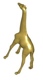
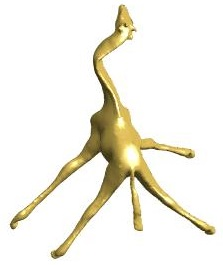
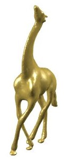
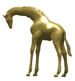
Canonical form
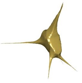
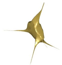
Paper
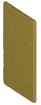
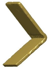
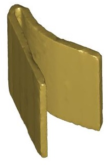
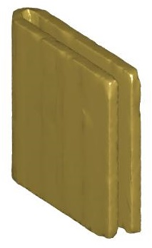
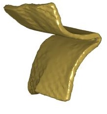
Canonical form
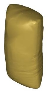
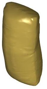
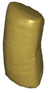
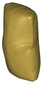
Watch
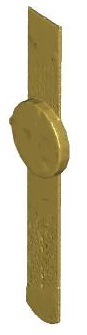
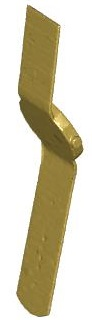
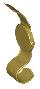
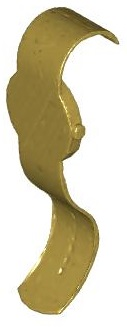
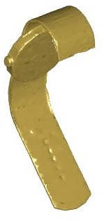
Canonical form

Figure 6: Shapes in different poses from the SHREC database, and their corresponding canonical forms obtained by NMDS. Here, each shape consists of $10^{4}$ vertices.

Unless a surface is an isometric deformation of another flat surface, flattening it into a canonical form would unavoidably involve some deformation of its intrinsic geometry. This deformation is termed the embedding error, which is defined by the value of the objective function of MDS,

$$\mbox{stress}(Z)=\left\|ZZ^{T}+\frac{1}{2}JEJ\right\|_{F}.$$ (39)

In our next experiment, shown in Figure 7, we compare the canonical forms of the giraffe and hand shapes, obtained using the different methods. For presentation purposes we scale each embedding error to $\frac{100}{p^{2}}\mbox{stress}(Z)$ and show it below its corresponding canonical form, where $p$ is the number of vertices. Qualitative and quantitative comparisons show that the proposed methods are similar to MDS in both minimizers and minima of the objective function. Additionally, the embedding results of NMDS are similar to those of MDS up to negligible differences.

	MDS	NMDS	FMDS	SMDS	Landmark	SSDE
Stress	5.355	5.355	5.366	5.557	6.288	10.748
Stress	3.883	3.887	3.936	4.472	9.128	11.191

Figure 7: Canonical forms of giraffe and hand shapes, using $n=100$ samples for the compared methods. The stress error $\frac{100}{p^{2}}{\left\|{Z{Z^{T}}+\frac{1}{2}JEJ}\right\|_{F}}$ of each embedding is displayed at the bottom of its corresponding form.

In our next experiment, we directly compare the canonical forms of the different methods ($Z$) to that of MDS ($Z^{*}$). To compare two canonical forms, we align them using ICP [4] and then compute the relative approximation error $\frac{\|Z-Z^{*}\|_{F}}{\|Z^{*}\|_{F}}$. Figure 8 shows the results with respect to the number of samples $n$, on the hand shape. It can be seen that both proposed methods outperform the others in approximating the embedding of MDS.

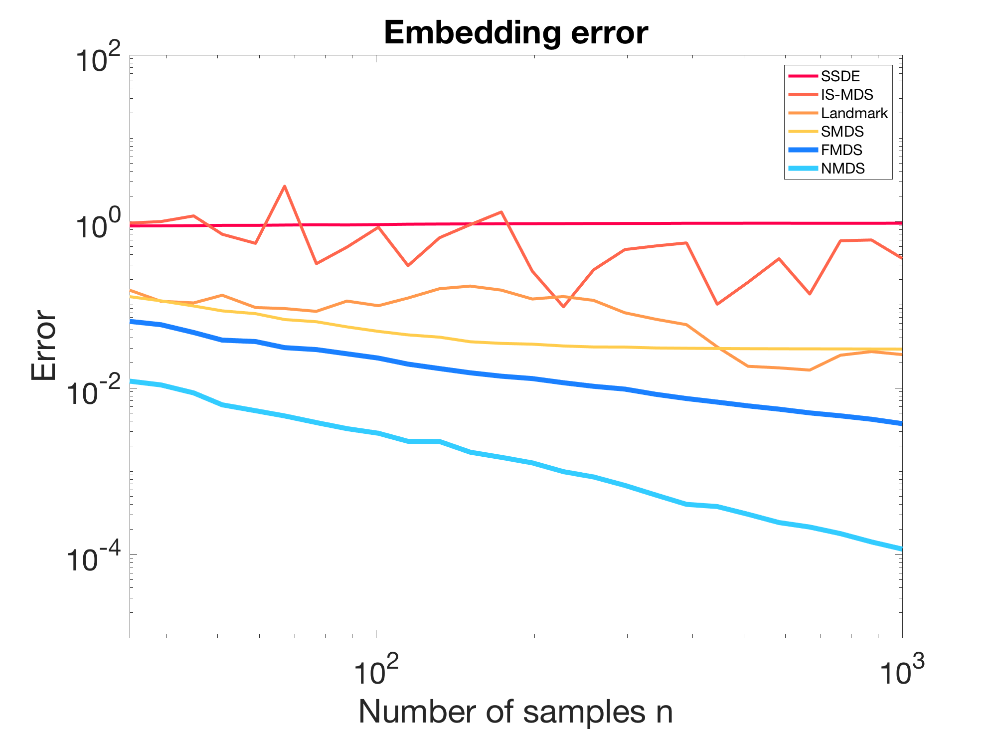
Figure 8: Distance of approximated canonical forms to the true one with respect the number of samples $n$, using different methods.

The proposed methods not only provide fast and accurate approximations compared to MDS, but can also be used to significantly accelerate the computation of geodesic distances by approximating them. In the following experiments, we measure the distance approximation error on the giraffe shape. In Figure 9, we compare the relative reconstruction error $\frac{\|\hat{D}-D\|_{F}}{\|D\|_{F}}$, where $\hat{D}$ approximates $D$ using different methods. Since the compared methods are essentially different low-rank approximations of $E$, we also add the best rank-$n$ approximation to the comparison.

Figure 9: The reconstruction error of $D$ with respect to the number of samples $n$, using different methods.

In Figure 10, we visualize the geodesics approximations of randomly chosen $30K$ pairs of distances using different methods. We do this by plotting the true and approximated distances along the $x$ and $y$ axes, thus showing the approximation’s distribution over the surface.

Figure 10: Approximated distance as a function of the true distance, using SMDS, FMDS, NMDS, Geodesics in Heat and the best low-rank reconstruction. For better visualization, the plots are shifted horizontally by $i=\{0,1,2,3\}$, respectively. In this experiment we used $n=100$.

Thus far, we used fast marching as a gold standard in order to compute the initial set of geodesic distances and then evaluate the results. In the following experiment, we use the exact geodesics method [38] instead. This method computes the exact geodesic paths on triangulated surfaces and is more accurate in terms of truncation error when compared to the limiting continuous solution. This should also allow us to compare our derived geodesic distances to the ones obtained using fast marching. Figure 11 shows that exact geodesic distances from less than $30$ points were required in the initialization step, in order to obtain a full matrix of pairwise geodesic distances, computed using NMDS, which is more accurate than the full matrix obtained by the fast marching method. This experiment demonstrates the average error.

Figure 11: The reconstruction error of $D$ with respect to the number of samples $n$ as evaluated by exact geodesics, using different methods.

In Table I we compare the preprocessing, query times and accuracies of CTP to the one proposed in this paper. We use the same Root-Mean-Square, over a set of random pairs, of the relative error $\epsilon(i,j)=\frac{\hat{D}(i,j)-D(i,j)}{D(i,j)}$, which was used in their paper. In this experiment, the initial set of distances was computed using fast marching for NMDS and FMDS, and exact geodesics for CTP. All three methods were evaluated using exact geodesics as the ground truth. The query time complexity is $O(1)$ for CTP and $O(n)$ for FMDS and NMDS, where $n=20$–$100$ is the number of samples. Nevertheless, in the method we propose, query operations are done by one matrix product that typically has efficient implementations in standard frameworks, and thus our query step is more than $\times 1000$ faster. As for the pre-processing step, the method we introduce requires many fewer samples (around $\times 100$ less geodesics computations) and is thus also much faster.

TABLE I: (a) Accuracy, (b) query, and (c) preprocessing time of geodesic distance approximations using FMDS, NMDS and CTP.

Next, we evaluate the influence of noise on the geodesic distance approximations. We add random uniform and sparse (salt and pepper) normally distributed noise to the hand and giraffe shapes, respectively. The sparse noise was added to $1\%$ of the vertices. We initialize NMDS and FMDS with the fast marching distances that were computed on the noisy surfaces, and evaluate the resulting geodesics using the fast marching distances that were computed before adding the noise. Figure 12 shows that the distances computed by our methods remain close to the noisy fast marching distances. Thus, we conclude that the methods we propose approximate the distances they were initialized with well, whether they contain noise or not.

Figure 12: Influence of noise on the geodesic approximation error for Geodesics in Heat, FMDS, NMDS, and fast marching. All approximations are compared to the geodesic distances that were computed using fast marching before adding the noise.

Next, we evaluate the deviation of the approximated distance from satisfying the triangle inequality, as done in [10]. We compute the total violation error of a surface point $a$ as follows. For any other two surface points $b,c$, if

$${\cal E}rr(a,b,c)=\|b-c\|-(\|b-a\|+\|c-a\|)$$ (40)

is positive, we add ${\cal E}rr(a,b,c)$ to the total violation error of point $a$. We choose $100$ random points on the surface and measure their total violation error. Figure 13 compares the NMDS, FMDS, and Heat methods. It can be seen that NMDS and FMDS had lower violation errors than Geodesics in Heat. Among the proposed methods, FMDS has the lowest error since it is more accurate than NMDS in approximating the small distances.

Figure 13: The triangle inequality total violation error of $100$ randomly chosen surface points (sorted), for NMDS, FMDS and Geodesics in Heat.

Finally, as shown in Figure 14, we evaluate the average computation time of MDS, NMDS, FMDS, and SMDS on three shapes from the TOSCA database [7], including the computation of the geodesic distances. We change the number of vertices $p$ by subsampling and re-triangulating the original shapes. The computations were evaluated on a 2.8 GHz i7 Intel computer with 16GB RAM. Due to time and memory limitations, MDS was computed only for small values of $p$.

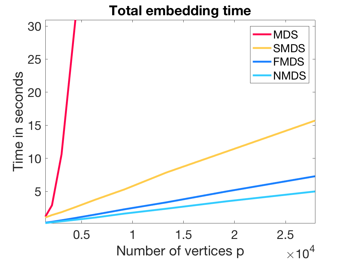
Figure 14: Average computation times (in seconds) for MDS, NMDS, FMDS and SMDS with respect to the number of vertices.

7 Sphere embedding

So far we discussed MDS as a flattening procedure, meaning that the data is embedded into a flat Euclidean space. Nevertheless, in some cases, it may be beneficial to embed the data onto a sphere, on which distances are measured according to the sphere’s metric. In this section, we extend the proposed methods for embedding onto a sphere rather than in a Euclidean space.

A $k$-dimensional sphere is the set of all points in $\mathbb{R}^{k+1}$ at an equal distance from a fixed point. Without loss of generality, we assume that this fixed point is the origin, so that the sphere is centered. The geodesic distance between two points $z_{i}$ and $z_{j}$ on a sphere of radius $r$ can be computed by the arc length

$$\frac{\alpha_{ij}}{2\pi}2\pi r=\alpha_{ij}r,$$ (41)

where $\alpha_{ij}$ is the angle between the vectors $z_{i},z_{j}$ in $\mathbb{R}^{k+1}$. Given a manifold with pairwise geodesic distances $D_{ij}$, we aim to find a set of points $\{z_{i}\}_{i=1}^{p}$ in $\mathbb{R}^{k+1}$, representing the embedding of the manifold on a sphere, such that $D_{ij}\approx\alpha_{ij}r$. Dividing by $r$ and applying $\cos$ on both sides leads to $\cos{\frac{D_{ij}}{r}}\approx\cos{\alpha_{ij}}$

Let $D$ be a $p\times p$ matrix holding the distances $D_{ij}$, and define $Z_{r}=\frac{1}{r^{2}}Z$. Since $\cos\alpha_{ij}=\frac{z_{i}^{T}z_{j}}{|z_{i}||z_{j}|}$, we can write in matrix formulation,

$$\cos\left(\frac{D}{r}\right)\approx Z_{r}Z_{r}^{T}.$$ (42)

Then, we can formulate the problem through the minimization

$$Z_{r}^{*}=\arg\min{\left\|{Z_{r}Z_{r}^{T}+E}\right\|_{F}},$$ (43)

similar to classical scaling, where $E=\cos(\frac{D}{r})$. This minimization can be solved using the same techniques presented in FMDS or NMDS. Namely, compute the decomposition of $E$ with one of the methods in Section 3. Then, follow Section 5 to obtain the truncated eigenvalue decomposition while ignoring the matrix $J$ and the scalar $\frac{1}{2}$. The final solution is given by $Z=r^{2}Z_{r}^{*}$.

A step of normalization of the rows of $Z_{r}^{*}$ can be added to constrain the points to lie on the sphere. Notice that when there exists an exact spherical solution, it will be obtained without this step. This results from the fact that $D_{ii}=0$ and, therefore, $E_{ii}=1$. Hence, for an exact solution without embedding errors, we get $\{Z_{r}Z_{r}^{T}\}_{ii}=1$, which is true only when the rows of $Z_{r}$ are normalized.

In the following experiment, a camera was located on a chair at the center of a room, and a video was taken while the chair was spinning. The frames of the video can be thought of as points in a high-dimensional space, lying on a manifold with a spherical structured intrinsic geometry. Using the method described in this section, we embed this manifold onto a $1$-dimensional sphere using NMDS (without the normalization step), and show the results in Figure 15. A nice visualization of this experiment appears in the supplementary material. Both MDS and NMDS result in a similar circular embedding, revealing the intrinsic geometry of the manifold. The pose of the camera for any frame can then be extracted from the embedding, even if the order of the frames in the video is unknown. This experiment also demonstrates that the proposed methods are capable of dealing with more complex manifolds in high-dimensional spaces and with embeddings in metrics other than Euclidean ones.

(a) MDS

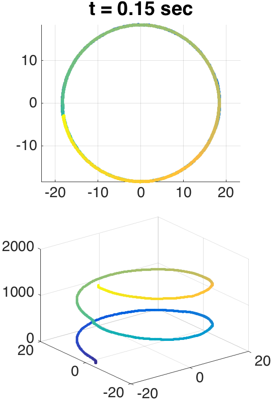
(b) NMDS

Figure 15: Embedding points onto a sphere using Full MDS (left) and the proposed NMDS (right). The points are frames of a video of a room taken from its center while rotating two whole turns. The images at the top show the embedding on a $1$-dimensional sphere. The time it took to create each embedding is added at the top. For better visualization, we add an additional axis of the frame number, shown in the images at the bottom.

Next, we randomly sample $p$ points $\{x_{i}\}_{1}^{p}$ from a quarter of a $k$-dimensional sphere of radius $r=1$, centered at the origin. We build a knn graph from the points such that each point is connected to $w$ neighbors. We compute $n$ initial geodesic distances both analytically and using Dijkstra’s shortest path for the farthest point sampling step, and approximate the rest of the distances using NMDS. Thereafter, we embed the distances on a $\tilde{k}$-dimensional sphere, as well as in a $\tilde{k}$-dimensional Euclidean space. For evaluation, we analytically compute all distances and compare them to the approximated ones using the relative reconstruction error seen previously in Figure 9. The embedding error is evaluated using the stress in Equation 39.

For this experiment, we choose $p=2000$ points, $n=100$ initial distances, embedding space dimension $\tilde{k}=2$, and $w=120$ nearest neighbors. Note, however, that the results did not change much for different sets of plausible parameters. We test the proposed method for different intrinsic dimensions $k$ between $1$ and $10$. Figure 16 shows the results. Not surprisingly, the stress is lower for sphere embedding than for Euclidean embedding. It can be seen that the proposed method approximates well both the ground truth embedding and the distances it was initialized with, regardless of the intrinsic dimension of the sphere manifold. For the distance approximation, the error of NMDS initialized by Dijkstra’s algorithm stems mainly from the error introduced by the graph approximating the continuous distance. As for the stress, since the embedding procedure is robust to noise in distances, the stress is not substantially different between the two proposed methods.

Figure 16: Evaluation of the proposed method with respect to the intrinsic dimension $k$. Top: The geodesic reconstruction error of Dijkstra’s algorithm, NMDS initialized by Dijkstra, and NMDS initialized by analytically computed distances. Bottom left: Stress error of embedding in a Euclidean space, using the distances computed analytically (True), with Dijkstra, and with NMDS initialized once with the analytic and then with the Dijkstra approximation of the distances. Bottom right: Stress error when embedding in a low-dimensional sphere.

8 Conclusions

In this paper we develop two methods for approximating MDS in its classical scaling version. In FMDS, following the ideas of Spectral-MDS, we interpolate the geodesic distances from a few samples using a smoothness assumption. This interpolation results in a product of small matrices that is a low-rank approximation of the distance matrix. Then, time and space complexities of MDS are significantly reduced by reformulating its minimization through the small matrices. The main contribution to the improvement in time complexity and accuracy over SMDS is the fact that we work entirely in the spacial domain, as opposed to SMDS, which translates the problem into the spectral domain and truncates the eigenspace. FMDS sets the stage for the second method we term NMDS. Instead of constructing an interpolation matrix using smoothness assumptions, it is now learned from the sampled data, which results in a different low-rank approximation of the distance matrix. A small modification of the method shows its relation to the Nyström approximation. Although NMDS performs better than FMDS in most experiments, the interpolation ideas of FMDS can also be used for other tasks, such as matrix completion, where instead of being arranged in columns, the known entries might be spread over the matrix. Experimental results show both methods achieve state-of-the-art results in canonical form computations. As a by-product, the methods we introduced can be used to compute geodesic distances on manifolds very fast and accurately. Finally, an extension to embedding on spheres shows how these methods can deal with more complex manifolds in high-dimensional space embedded into non-flat metric spaces.

9 Acknowledgements

The research leading to these results has received funding from the European Research Council under European Union’s Seventh Framework Programme, ERC Grant agreement no. 267414

Gil Shamai is a PhD candidate at the Geometric Image Processing (GIP) laboratory, at the Technion—Israel Institute of Technology. Shamai is a veteran of the Technion undergraduate Excellence Program and his research was recognized by being the recipient of several awards, including the Meyer Prize, Finzi Prize, and Sherman Interdisciplinary Graduate School Fellowship. His main interests are theoretical and computational methods in metric geometry and their application to problems in manifold learning, multidimensional scaling procedures and fast geodesics computation, as well as medical imaging and machine learning.

Michael Zibulevsky received his MSc in Electrical Engineering from MIIT—Transportation Engineering Institute, Moscow and DSc in Operations Research from the Technion—Israel Institute of Technology (1996). He is currently with the Computer Science Department at the Technion. Dr. Zibulevsky is one of the original developers of Sparse Component Analysis. His research interests include numerical methods of nonlinear optimization, sparse signal representations, deep neural networks and their applications in signal / image processing and inverse problems.

Ron Kimmel is a Professor of Computer Science at the Technion where he holds the Montreal Chair in Sciences. He has worked in various areas of image processing and analysis in computer vision, image processing, and computer graphics. Kimmel’s interest in recent years has been shape reconstruction, analysis and learning, medical imaging and computational biometry, and applications of metric and differential geometries. He is an IEEE Fellow, recipient of the Helmholtz Test of Time Award, and the SIAG on Imaging Science Best Paper Prize. At the Technion he founded and heads the Geometric Image Processing (GIP) Laboratory. He also served as the Vice Dean for Teaching Affairs, and Vice Dean for Industrial Relations. Currently, he serves as Head of Academic Affairs of the Technion’s graduate interdisciplinary Autonomous Systems Program (TASP). Since the acquisition of InVision (a company he co-founded) by Intel in 2012, he has also been heading a small R&D team as part of Intel’s RealSense.

References

- [1] Y. Aflalo and R. Kimmel. Spectral multidimensional scaling. Proceedings of the National Academy of Sciences, 110(45):18052–18057, 2013.
- [2] N. Arcolano and P. J. Wolfe. Nyström approximation of wishart matrices. In Acoustics Speech and Signal Processing (ICASSP), 2010 IEEE International Conference on, pages 3606–3609. IEEE, 2010.
- [3] M. Belkin and P. Niyogi. Laplacian eigenmaps and spectral techniques for embedding and clustering. In NIPS, volume 14, pages 585–591, 2001.
- [4] Paul J Besl and Neil D McKay. Method for registration of 3-d shapes. In Robotics-DL tentative, pages 586–606. International Society for Optics and Photonics, 1992.
- [5] I. Borg and P. J. Groenen. Modern multidimensional scaling: Theory and applications. Springer, 2005.
- [6] Mario Botsch and Olga Sorkine. On linear variational surface deformation methods. IEEE transactions on visualization and computer graphics, 14(1):213–230, 2008.
- [7] A. M. Bronstein, M. M. Bronstein, and R. Kimmel. Numerical geometry of non-rigid shapes. Springer, 2008.
- [8] Marcel Campen and Leif Kobbelt. Walking on broken mesh: Defect-tolerant geodesic distances and parameterizations. In Computer Graphics Forum, volume 30, pages 623–632. Wiley Online Library, 2011.
- [9] A. Civril, M. Magdon-Ismail, and E. Bocek-Rivele. SSDE: Fast graph drawing using sampled spectral distance embedding. In Graph Drawing, pages 30–41. Springer, 2007.
- [10] Keenan Crane, Clarisse Weischedel, and Max Wardetzky. Geodesics in heat: A new approach to computing distance based on heat flow. ACM Transactions on Graphics (TOG), 32(5):152, 2013.
- [11] E. W. Dijkstra. A note on two problems in connexion with graphs. Numerische Mathematik l, pages 269–27.
- [12] D. L. Donoho and C. Grimes. Hessian eigenmaps: Locally linear embedding techniques for high-dimensional data. Proceedings of the National Academy of Sciences, 100(10):5591–5596, 2003.
- [13] P. Drineas, R. Kannan, and M. W. Mahoney. Fast monte carlo algorithms for matrices iii: Computing a compressed approximate matrix decomposition. SIAM Journal on Computing, 36(1):184–206, 2006.
- [14] H. A. Drury, D. C. Van Essen, C. H. Anderson, C. W. Lee, T. A. Coogan, and J. W. Lewis. Computerized mappings of the cerebral cortex: a multiresolution flattening method and a surface-based coordinate system. Journal of cognitive neuroscience, 8(1):1–28, 1996.
- [15] A. Elad and R. Kimmel. On bending invariant signatures for surfaces. Pattern Analysis and Machine Intelligence, IEEE Transactions on, 25(10):1285–1295, 2003.
- [16] Haw-ren Fang and Dianne P O’Leary. Euclidean distance matrix completion problems. Optimization Methods and Software, 27(4-5):695–717, 2012.
- [17] D. S. Hochbaum and D. B. Shmoys. A best possible heuristic for the k-center problem. Mathematics of operations research, 10(2):180–184, 1985.
- [18] R. Kimmel and J. A. Sethian. Computing geodesic paths on manifolds. Proceedings of the National Academy of Sciences, 95(15):8431–8435, 1998.
- [19] T. Kohonen. The self-organizing map. Neurocomputing, 21(1):1–6, 1998.
- [20] Z. Lian, J. Zhang, S. Choi, H. ElNaghy, J. El-Sana, T. Furuya, A. Giachetti, R. A. Guler, L. Lai, C. Li, H. Li, F. A. Limberger, R. Martin, R. U. Nakanishi, A. P. Neto, L. G. Nonato, R. Ohbuchi, K. Pevzner, D. Pickup, P. Rosin, A. Sharf, L. Sun, X. Sun, S. Tari, G. Unal, and R. C. Wilson. Non-rigid 3D Shape Retrieval. In I. Pratikakis, M. Spagnuolo, T. Theoharis, L. Van Gool, and R. Veltkamp, editors, Eurographics Workshop on 3D Object Retrieval. The Eurographics Association, 2015.
- [21] Yaron Lipman, Raif M Rustamov, and Thomas A Funkhouser. Biharmonic distance. ACM Transactions on Graphics (TOG), 29(3):27, 2010.
- [22] R. Liu, V. Jain, and H. Zhang. Sub-sampling for efficient spectral mesh processing. In Advances in Computer Graphics, pages 172–184. Springer, 2006.
- [23] M. W. Mahoney and P. Drineas. CUR matrix decompositions for improved data analysis. Proceedings of the National Academy of Sciences, 106(3):697–702, 2009.
- [24] Daniele Panozzo, Ilya Baran, Olga Diamanti, and Olga Sorkine-Hornung. Weighted averages on surfaces. ACM Transactions on Graphics (TOG), 32(4):60 2013.
- [25] Ulrich Pinkall and Konrad Polthier. Computing discrete minimal surfaces and their conjugates. Experimental mathematics, 2(1):15–36, 1993.
- [26] John C Platt. Fastmap, metricmap, and landmark mds are all Nyström algorithms. In Proc. 10th Int. Workshop on Artificial Intelligence and Statistics, pages 261–268, 2005.
- [27] R. Pless. Image spaces and video trajectories: Using isomap to explore video sequences. In ICCV, volume 3, pages 1433–1440, 2003.
- [28] S. T. Roweis and L. K. Saul. Nonlinear dimensionality reduction by locally linear embedding. Science, 290(5500):2323–2326, 2000.
- [29] Y. Rubner and C. Tomasi. Perceptual metrics for image database navigation. Springer, 2000.
- [30] B. Schölkopf, A. Smola, and K. Müller. Nonlinear component analysis as a kernel eigenvalue problem. Neural computation, 10(5):1299–1319, 1998.
- [31] E. L. Schwartz, A. Shaw, and E. Wolfson. A numerical solution to the generalized mapmaker’s problem: flattening nonconvex polyhedral surfaces. Pattern Analysis and Machine Intelligence, IEEE Transactions on, 11(9):1005–1008, 1989.
- [32] H. Schweitzer. Template matching approach to content based image indexing by low dimensional euclidean embedding. In Computer Vision, 2001. ICCV 2001. Proceedings. Eighth IEEE International Conference on, volume 2, pages 566–571. IEEE, 2001.
- [33] Gil Shamai, Yonathan Aflalo, Michael Zibulevsky, and Ron Kimmel. Classical scaling revisited. In Proceedings of the IEEE International Conference on Computer Vision, pages 2255–2263, 2015.
- [34] Gil Shamai and Ron Kimmel. Geodesic distance descriptors. In Proceedings of the IEEE Conference on Computer Vision and Pattern Recognition, pages 6410–6418, 2017.
- [35] Gil Shamai, Michael Zibulevsky, and Ron Kimmel. Accelerating the computation of canonical forms for 3d nonrigid objects using multidimensional scaling. In Proceedings of the 2015 Eurographics Workshop on 3D Object Retrieval, pages 71–78. Eurographics Association, 2015.
- [36] V. D Silva and J. B. Tenenbaum. Global versus local methods in nonlinear dimensionality reduction. In Advances in neural information processing systems, pages 705–712, 2002.
- [37] Oded Stein, Eitan Grinspun, Max Wardetzky, and Alec Jacobson. Natural boundary conditions for smoothing in geometry processing. ACM Transactions on Graphics (TOG), 37(2):23, 2018.
- [38] Vitaly Surazhsky, Tatiana Surazhsky, Danil Kirsanov, Steven J Gortler, and Hugues Hoppe. Fast exact and approximate geodesics on meshes. In ACM transactions on graphics (TOG), volume 24, pages 553–560. Acm, 2005.
- [39] Joshua B Tenenbaum, Vin De Silva, and John C Langford. A global geometric framework for nonlinear dimensionality reduction. Science, 290(5500):2319–2323, 2000.
- [40] Shi-Qing Xin, Xiang Ying, and Ying He. Constant-time all-pairs geodesic distance query on triangle meshes. In Proceedings of the ACM SIGGRAPH symposium on interactive 3D graphics and games, pages 31–38. ACM, 2012.
- [41] H. Yu, X. Zhao, X. Zhang, and Y. Yang. ISOMAP using Nyström method with incremental sampling. Advances in Information Sciences & Service Sciences, 4(12), 2012.
- [42] Kai Yu, Tong Zhang, and Yihong Gong. Nonlinear learning using local coordinate coding. In Advances in neural information processing systems, pages 2223–2231, 2009.
- [43] Yin Zhou and Kenneth E Barner. Locality constrained dictionary learning for nonlinear dimensionality reduction. Signal Processing Letters, IEEE, 20(4):335–338, 2013.
- [44] Gil Zigelman, Ron Kimmel, and Nahum Kiryati. Texture mapping using surface flattening via multidimensional scaling. Visualization and Computer Graphics, IEEE Transactions on, 8(2):198–207, 2002.