Relaxed Earth Mover’s Distances for Chain- and Tree-connected Spaces
and their use as a Loss Function in Deep Learning

Abstract

The Earth Mover’s Distance (EMD) computes the optimal cost of transforming one distribution into another, given a known transport metric between them. In deep learning, the EMD loss allows us to embed information during training about the output space structure like hierarchical or semantic relations. This helps in achieving better output smoothness and generalization. However EMD is computationally expensive. Moreover, solving EMD optimization problems usually require complex techniques like lasso. These properties limit the applicability of EMD-based approaches in large scale machine learning.

We address in this work the difficulties facing incorporation of EMD-based loss in deep learning frameworks. Additionally, we provide insight and novel solutions on how to integrate such loss function in training deep neural networks. Specifically, we make three main contributions: (i) we provide an in-depth analysis of the fastest state-of-the-art EMD algorithm (Sinkhorn Distance) and discuss its limitations in deep learning scenarios. (ii) we derive fast and numerically stable closed-form solutions for the EMD gradient in output spaces with chain- and tree- connectivity; and (iii) we propose a relaxed form of the EMD gradient with equivalent computational complexity but faster convergence rate. We support our claims with experiments on real datasets. In a restricted data setting on the ImageNet dataset, we train a model to classify 1000 categories using 50K images, and demonstrate that our relaxed EMD loss achieves better Top-1 accuracy than the cross entropy loss. Overall, we show that our relaxed EMD loss criterion is a powerful asset for deep learning in the small data regime.

Figure 1: We train a deep learning model using Ellyvan (a hybrid elephant and van). The output of the forward pass is presented in the first row, and the label in the second. The tree-structured output space allows us to train the network using gradients from the Earth Mover’s Distance ($\nabla\emph{EMD}$). We introduce a regularized form that converges faster ($\nabla\emph{EMD}^{2}$) and is more stable.

1 Introduction

The Wasserstein metric [33] is a distance function based on the optimal transport problem that compares two data distributions. While computing such metrics on digital devices, it is common practice for data distributions to work in a discretized space (e.g. arranged in bins). Here, the Wasserstein distance is popularly known as the Earth Mover’s Distance (EMD) [24]. The name is derived from a visual analogy of the data distributions as two piles of dirt (earth). EMD is defined as the minimum amount of effort required to make both distributions look alike. Note that the individual bins of both distributions should be non-negative and their total mass equal (as is the case with probability distributions).

The EMD is widely used to compare histograms and probability distributions [16, 20, 23, 24, 25]. However, calculating the EMD is known to be computationally expensive. This has led to several relaxed versions of the EMD for cases where speed is critical, e.g. when comparing feature vectors [14, 19, 21].

In addition to the large computational cost, EMD has the drawback of an $\ell_{1}$ behavior. Solving EMD optimization problems often require lasso optimization techniques (e.g., mirror descent, Bregman projections, etc.). This represents a significant drawback for current deep learning approaches that strongly favor gradient-based methods such as Stochastic Gradient Descent, Momentum [31], and Adam [2], that provide several small updates to the model parameters.

Sinkhorn Distance. Using the EMD within an iterative optimization scheme was made feasible by Cuturi [7], who realized that an entropically regularized EMD can be efficiently calculated using the Sinkhorn-Knopp [27] algorithm. The resulting is referred to as the Sinkhorn Distance (SD), and has achieved wide popularity within a number of learning frameworks [3, 4, 9, 10, 18, 22, 23, 28, 29, 30]. The SD approximates EMD effectively, and provides a subgradient for the EMD as a side result of the estimation. This SD subgradient has been used to train deep learning models [10] and is implemented as a loss criterion in popular deep frameworks such as Caffe [12] and Mocha [1]. However, as SD is an $\ell_{1}$ norm, Frogner et al. [10] need to combine SD with the Küllback-Leibler divergence and use an exceedingly small learning rate for it to converge.

Furthermore, the SD algorithm is prone to numerical instabilities when used in deep learning frameworks. In some conditions, these instabilities imply that SD is not a close approximation of EMD. We believe that an analysis of the causes of instabilities is critical to extend the use of SD to deep learning frameworks and discuss them in detail in Sec. 2.

Earth Mover’s Distance. Concurrently, we suggest an alternative approach to SD. Instead of tackling the general case, we focus on output spaces whose connectivity graph takes the form of a chain (histograms or probability distributions) or a tree (hierarchies). We provide closed-form solutions for the real EMD and its gradient.

We start with chain-connected distributions (see Fig. 4) that have a well-known closed-form solution [32], and derive its gradient. We also propose a relaxed version of the EMD, named $\emph{EMD}^{2}$ that exhibits similar structure but converges faster due to its $\ell_{2}$ behavior.

Furthermore, we derive a closed form solution for the EMD and its gradient that is valid for all metric spaces that have a tree connectivity graph. This allows us to represent complex output spaces that are hierarchical in nature (e.g., WordNet [17] and ImageNet [26], Sentence Parse Trees [15]). We see an example of a hierarchical output space of object categories in Fig. 1. We depict the expected flow of dirt on the tree branches, and present the gradients for both original and relaxed versions of the EMD (details of the gradients in Sec. 3.2 and Sec. 4).

EMD as a loss criterion for deep learning. Using EMD as a loss criterion has several unique advantages over unstructured losses. It allows us to shape the output relationships we expect from a model. For example, it can tell the model that confusing a cat for a tiger may more acceptable than confusing a cat for a starship, and thus adds knowledge to the model. Additionally, EMD gradients (in contrast to MSE) are holistic and affect the whole output space as it is connected. Therefore, models that predict the entire output space (e.g., histograms) converge faster.

Overall, we see that EMD has the effect of magnifying the information that an input data sample provides. Each input sample does not only provide information about its own class, but also contains the relationship it has with the rest of the output bins (e.g., classes, histogram bins, etc.) This second source of information helps generalize better, and results in improved performance with less data.

We demonstrate these characteristics in two real-world experiments. We train a model to predict the Power Spectral Density of respiratory signals of sleep laboratory patients. In this setting the EMD converges faster than the SD and MSE losses, and achieves better accuracy. Our second experiment is performed on a reduced version of the ILSVRC 2012 challenge [26]. We use all 1000 categories, but limit the training data to 50K images. This, along with the EMD criterion, forces the network to learn the output space hierarchy. While EMD alone is not enough to achieve the best top-1 accuracy, an equal combination of EMD and cross entropy loss achieves better top-1 accuracy than using cross entropy alone.

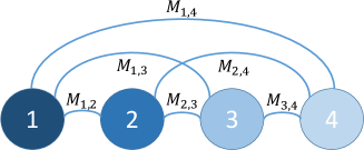
Figure 2: We illustrate the general case of the EMD, where the dirt can be moved from and to all bins directly. Computing the amount of dirt that goes (flows) through each path is computationally expensive.

(a) Ratio of distances vs. Sinkhorn-Knopp iterations

(b) Ratio of distances vs. Floating point representation

(c) Angle between gradients vs. Sinkhorn-Knopp iterations

(d) Angle between gradients vs. Floating point representation

Figure 3: We show how implementation and hyper-parameter choices affect SD with an experiment on the WordNet hierarchy for 1000 ImageNet classes. (a,b): Ratio of SD to the real EMD. (c,d): Angle of the cosine distance $\left(D_{C}(\cdot,\cdot)\right)$ between EMD and SD gradients. (a,c): Impact of limiting Sinkhorn-Knopp iterations. We see that larger values of $\lambda$ require a large amount of iterations to converge (two typical values used in deep learning are 10 [10] and 100 [12]). (b,d): float32 (GPU) has a reduced dynamic range compared to float64 (CPU), which degenerates for large $\lambda$ values. The gray dashed line shown as a reference, corresponds to $10000$ iterations using float64 representation. The most commonly cited value of $\lambda$ is 10.

2 The Earth Mover’s Distance

As discussed earlier, the EMD is defined for discrete distributions. Here, the probability mass (or dirt) is distributed in discrete piles or bins. The effort of moving a mound of dirt between two bins is a non-negative cost which is linearly proportional to the amount of dirt and distance between the bins.

Within this discrete domain, the general form of EMD between two distributions $\mathbf{p},\mathbf{q}\in\mathbb{R}^{N}_{+}$ with $\left\lVert\mathbf{p}\right\rVert_{1}=\left\lVert\mathbf{q}\right\rVert_{1}$ is

$$\emph{EMD}(\mathbf{p},\mathbf{q})=\inf_{T\in U(\mathbf{p},\mathbf{q})}\langle M,T\rangle\,,$$ (1)

where $\langle\cdot,\cdot\rangle$ is the Frobenius inner product and $M\in\mathbb{R}^{N\times N}_{+}$ defines the generalized distance between bins (see Fig. 2). $U(\mathbf{p},\mathbf{q})$ is the set of valid transport plans between $\mathbf{p}$ and $\mathbf{q}$,

$$U(\mathbf{p},\mathbf{q})=\{T\in\mathbb{R}^{N\times N}_{+}:T\cdot\mathbf{1}_{N}=\mathbf{p},\,T^{\top}\cdot\mathbf{1}_{N}=\mathbf{q}\}\,.$$ (2)

$\mathbf{1}_{N}$ is an $N$ dimensional vector of all ones, and $T$ is constrained such that its row sum corresponds to the distribution $\mathbf{p}$ and column sum to $\mathbf{q}$.

Without loss of generality (a simple scalar normalization), in the rest of the paper we assume $\left\lVert\mathbf{p}\right\rVert_{1}=\left\lVert\mathbf{q}\right\rVert_{1}=1$.

2.1 Unnormalized distributions

The original EMD is not defined for $\left\lVert\mathbf{p}\right\rVert_{1}\neq\left\lVert\mathbf{q}\right\rVert_{1}$. Although there are several ways to modify the EMD for unnormalized distributions [5, 10, 19] we consider that this goes against the spirit of the metric. Therefore, prior to computing the EMD, we $\ell_{1}$-normalize the input distributions either using a $\ell_{1}$ normalization layer, or a softmax layer.

2.2 Sinkhorn distance

The general formulation of the EMD (Eq. 1) is solved using linear programming which is computationally expensive. However, this problem was greatly alleviated by Cuturi [7] who suggested a smoothing term for the EMD in the form of

$$\emph{SD}_{\lambda}(\mathbf{p},\mathbf{q})=\inf_{T\in U(\mathbf{p},\mathbf{q})}\langle M,T\rangle-\frac{1}{\lambda}\langle T,\log T\rangle\,,$$ (3)

which allows to use the Sinkhorn-Knopp algorithm [27] to obtain an iterative and efficient solution.

The Sinkhorn-Knopp algorithm is notable as it converges fast and produces a subgradient for the SD without extra cost. This subgradient can in turn be used to update parameters of machine learning models [10]. The algorithm is defined as:

Algorithm 1 Sinkhorn Distance and Gradient

0:  $f(x),y,\lambda,\mathbf{M}$

  $\mathbf{K}\leftarrow e^{-\lambda\mathbf{M}-1}$, $u\leftarrow\mathbf{1}$, $it\leftarrow 1$

  while not converged and it $\leq$ MAX-ITER do

     $u\leftarrow f(x)\oslash\left(\mathbf{K}(y\oslash\mathbf{K}^{\top}u)\right)$

  end while

  $v\leftarrow y\oslash(\mathbf{K}^{\top}u)$

  $\emph{SD}\leftarrow\text{sum}(u\odot(\mathbf{K}\odot\mathbf{M}v))$

  $\nabla\emph{SD}\leftarrow\log{u}/\lambda$

2.3 Numerical stability of the Sinkhorn Distance

We claim that the SD is not numerically stable when used in common deep learning frameworks. We substantiate this claim by comparing the output of the SD and its gradient to the real EMD. We extract a hierarchy of categories from the WordNet ontology for the 1000 classes of the ILSVRC2012 dataset [26]. The tree has 1374 nodes in total. This hierarchy acts as the structure of the output space in our evaluation.

There are three parameters that impact numerical stability of the SD in deep learning:

Iteration limit:

any practical implementation needs an upper limit for the number of SD iterations. This leads to a trade-off between speed and accuracy which is more apparent for larger values of $\lambda$, as seen in Fig. 3 (a), (c).

Floating point accuracy:

the Sinkhorn algorithm alternately normalizes rows and columns of the transport matrix. This requires several multiply-accumulate operations which are prone to numerical inaccuracies. This problem is made worse by the exponential form of $\mathbf{K}=e^{-\lambda\mathbf{M}-1}$, which increases the dynamic range of the values. To make things worse, GPUs use a float32 representation, instead of the common float64 representation used by CPUs. In Fig. 3 (b) and (d), we observe how using float32 affects the results, especially for large values of $\lambda$ where more iterations are required to converge.

Regularization factor ($\lambda$):

the regularization factor affects both the accuracy and the convergence behavior of SD. In a non-deep learning framework, the number of iterations does not pose a limit and float64 representation can be used. Lower values of $\lambda$ imply better convergence behavior [8], while larger values approximate the Earth Mover’s Distance better (see gray reference line in Fig. 3). However, in deep learning applications where float32 representation are common and the iteration number is typically chosen to be $10$ [10] or $100$ [12], larger values of $\lambda$ are unusable.

In general, SD works best when the ratio between the largest and the smallest non-zero value in the $\mathbf{M}$ is small (thus has a smaller dynamic range), and the size of the output space is small (due to the reduced number of multiply-add operations).

(a) Chain EMD

Figure 4: One dimensional probability distributions are a perfect example of chain output spaces. In chains, dirt must travel through all intermediate bins in its path. This greatly simplifies the computation of the EMD, as it only requires to eliminate one node and edge at each step.

3 EMD in chain-connected spaces

We analyze the scenario where bins in a distributions (e.g. histograms, probabilities) are situated in a one dimensional space. Here, moving dirt from a source to target bin requires an ordered visit to every bin in between (see Fig. 4).

The bin distance $M$ can be defined recursively to ensure that only consecutive bin distances are considered.

$$M_{i,j}=\begin{cases}0&\text{if }i=j\,,\\ M_{i-1,j}+d_{i-1,i}&\text{if }i>j\,,\\ M_{j,i}&\text{if }i<j\,.\end{cases}$$ (4)

Here, $d_{i-1,i}$ is the distance between two consecutive bins (typically all equal and $1$).

The above choice of bin distances facilitates a simple solution to calculate the EMD using a recursion. Essentially, each bin either receives all the excess dirt that results from leveling previous bins, or in case of a deficit, tries to provide for it. Note that the cost of going left-to-right ($M_{i,j}$) or right-to-left ($M_{j,i}$) is symmetric. The closed form recursive formulation for the EMD between two one-dimensional distributions is:

$$\overrightarrow{\emph{EMD}}(\mathbf{p},\mathbf{q})=\sum_{i=1}^{N-1}M_{i,i+1}\cdot|\varphi_{i}|\,,$$ (5)

where $\varphi_{i}$ represents the excess dirt that needs to be moved ahead or deficit in dirt that needs to be filled up to bin $i$.

$$\varphi_{i}=\sum_{j=1}^{i}\left(p_{j}-q_{j}\right)\,.$$ (6)

For notational brevity, we will refer to $M_{i,i+1}$ as $\hat{M}_{i}$. The above expression can be rewritten with the sign function as

$$\overrightarrow{\emph{EMD}}(\mathbf{p},\mathbf{q})=\sum_{i=1}^{N-1}\hat{M}_{i}\cdot\text{sgn}(\varphi_{i})\cdot\varphi_{i}\,.$$ (7)

Note that as both distributions have the same amount of total mass, and we progressively level out the dirt over all bins, when we arrive to the last bin all dirt will have been leveled (i.e. $\varphi_{N}=0$). Therefore, we compute the outer sum only up to $N-1$.

3.1 Gradient of the Earth Mover’s Distance

To integrate EMD as a loss function in an iterative gradient-based optimization approach, we need to compute the analytical form of the gradient. However, we must ensure that the gradient obeys the law of dirt conservation. The gradient should not create new or destroy existing dirt to avoid changing the total mass of the distributions ($\left\lVert\mathbf{p}\right\rVert_{1}\neq 1$ after updates).

We use the trick of projected gradients, and define $\mathbf{e}_{k}$ as a vector of length $N$ whose value at entry $k$ is $1-1/N$, and $-1/N$ elsewhere. Note that $\mathbf{e}_{k}$ sums to $0$. For a small value $h$, we compute the distance between the perturbed distribution $\mathbf{p}+h\mathbf{e}_{k}$ and $\mathbf{q}$ as:

$$\begin{split}&\overrightarrow{\emph{EMD}}(\mathbf{p}+h\mathbf{e}_{k},\mathbf{q})\simeq\\ &\sum_{i=1}^{N-1}\hat{M}_{i}\cdot\text{sgn}(\varphi_{i})\sum_{j=1}^{i}\left(p_{j}+h(\delta_{jk}-1/N)-q_{j}\right)\,,\end{split}$$ (8)

where $\delta_{jk}=1$ iff $j=k$. Note that by choosing $h$ small enough, $\text{sgn}(\varphi_{i})$ can be assumed to remain unchanged. The corresponding partial derivative for the $\overrightarrow{\emph{EMD}}$ is:

$$\frac{\partial\overrightarrow{\emph{EMD}}({\mathbf{p}},{\mathbf{q}})}{\partial p_{k}}\simeq\sum_{i=1}^{N-1}\hat{M}_{i}\cdot\text{sgn}(\varphi_{i})\sum_{j=1}^{i}\left(\delta_{jk}-1/N\right)\,.$$ (9)

3.2 Relaxed Earth Mover’s Distance

The proposed gradient (Eq. 9) is numerically stable and avoids erosion or addition of new dirt. This is an important step forward to use EMD in learning frameworks.

However, as the distance contains an absolute value function ($|\varphi_{i}|$) we observe difficulties converging to a solution, similar to $\ell_{1}$ optimization. In particular, when $\hat{M}_{i}\in\mathbb{N}$, it is easy to see that the terms of $\nabla\emph{EMD}$ are integer fractions of $N$ (see Fig. 1, multiples of 0.25). Furthermore, as small changes to the distribution do not change the gradient, the Hessian is zero except at a few discrete set of points (where the sign of $\varphi_{i}$ changes) making optimization hard.

To solve these issues, we suggest a relaxed form of the EMD where the cost is calculated proportional to a power of the excess/deficit of dirt.

$$\overrightarrow{\emph{EMD}}^{\rho}(\mathbf{p},\mathbf{q})=\sum_{i=1}^{N-1}\hat{M}_{i}\cdot|\varphi_{i}|^{\rho}\,.$$ (10)

whose gradient is:

$$\nabla\overrightarrow{\emph{EMD}}^{\rho}\simeq\rho\sum_{i=1}^{N-1}\hat{M}_{i}\cdot\varphi_{i}\cdot|\varphi_{i}|^{\rho-2}\sum_{j=1}^{i}\left({\delta_{jk}-1/N}\right)\,.$$ (11)

For $\rho=1$ we have the normal EMD distance, which behaves like $\ell_{1}$. During gradient descend we suggest to use the case with $\rho=2$ that bears similarity with the popular Mean Squared Error loss. $\emph{EMD}^{2}$ preserves the nice properties of conserving dirt, while having real valued gradients (see an example in Fig. 1). In addition, we see that $\overrightarrow{\emph{EMD}}^{2}$ also exhibits non-zero Hessians.

$$\begin{split}\frac{\partial^{2}\overrightarrow{\emph{EMD}}^{2}({\mathbf{p}},{\mathbf{q}})}{\partial p_{k}\partial p_{l}}=2\sum_{i=1}^{N-1}\hat{M}_{i}&\cdot(N\cdot H(i-l)-i)\\ &\cdot(N\cdot H(i-k)-i)\,,\end{split}$$ (12)

where $H:\mathbb{R}\rightarrow\{0,1\}$ is the Heaviside step function defined as $H(n)=\{1\text{ if }n\geq 0,0\text{ otherwise}\}.$

3.3 Discussion: comparing EMD, SD and MSE

Plotting the gradients provides a good impression of the actual behavior of the EMD. It also shows how EMD serves as a criterion that provides holistic optimization over the output space (full distribution).

In Fig. 5 we show the gradients corresponding to several different loss criteria for the transformation between two unit-norm distributions: a smooth one $\mathbf{p}$, and a spiky one $\mathbf{q}$. We present the gradient of MSE in Fig. 5 (a). Note how MSE optimizes each bin independently, and results in a non-smooth gradient.

In Fig. 5 (b) we show the gradients for EMD and $\emph{EMD}^{2}$. In both cases the gradient is holistic and affects the whole output space. Furthermore, the regularization effect induced by $\emph{EMD}^{2}$ results in a smoother gradient.

In Fig. 5 (c) we show the SD gradient for $\lambda$ values of 0.5, 1 and 10. In all cases the gradients are also holistic. We see that that larger values of $\lambda$ produce a gradient resembling that of the true EMD, however it comes with its own set of problems that were discussed earlier.

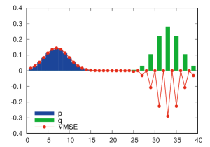
(a) Mean Squared Error

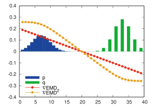
(b) Earth Mover’s Distance

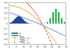
(c) Sinkhorn Distance

Figure 5: Gradient flow to convert a source distribution $\mathbf{p}$ to a target $\mathbf{q}$. (a) MSE gradient is not smooth, and does not affect the whole output space. (b) EMD and $\emph{EMD}^{2}$ gradients affect the whole space. $\emph{EMD}^{2}$ has $\ell_{2}$ behavior, while EMD behaves like $\ell_{1}$. (c) SD gradients also affect the whole space but the regularized versions are asymmetric. $\emph{SD}_{\lambda=10}$ approximates EMD well.

4 EMD in tree-connected spaces

We demonstrate here how EMD can be used to model output spaces with a tree structure. Our formulation expects that all observed bins correspond to the leaves of the tree, and the remaining latent nodes and have no dirt. As we can link a tree to any non-leaf node with a zero-cost connection, this formulation allows us to express any tree structure. We refer to this analysis as the Hierarchical Earth Mover’s Distance (HEMD) (see Fig. 1). Note that, this is still compatible with all our previous developments (as chains are a sub-class of trees). As such, we do not distinguish between EMD and HEMD while presenting the evaluation.

We define $\emph{HEMD}^{\rho}$ as:

$$\emph{HEMD}^{\rho}(\mathbf{p},\mathbf{q})=\sum_{i\in G}M_{i,\mathbf{p}(i)}\cdot|\tilde{\varphi}_{i}|^{\rho},\text{ where }$$ (13)

$$\tilde{\varphi}_{i}=\sum_{j\in\mathbf{l}(i)}\left(p_{j}-q_{j}\right)\,,$$ (14)

where $M_{i,\mathbf{p}(i)}$ is the cost of transporting dirt from node $i$ to its parent (abbreviated as $\tilde{M}_{i}$), $G$ is the set of all nodes in the tree, and $\mathbf{l}(i)$ is the set of all leaves in the subtree that has $i$ as a root. $N$ is the total number of leaves (and bins) in the tree. The intuition behind this formula is that we can reduce the tree one leave at a time as if it were the tail of a chain.

Then the gradient of HEMD is defined as:

$$\nabla\emph{HEMD}^{\rho}\simeq\rho\sum_{i\in G}\tilde{M}_{i}\cdot\tilde{\varphi}_{i}\cdot|\tilde{\varphi}_{i}|^{\rho-2}\sum_{j=1}^{i}\left({\delta_{jk}-1/N}\right)\,.$$ (15)

All equations can be solved efficiently by a post-order traversal of nodes in the tree.

5 Experimental analysis

We implement our models, the EMD and the SD criterions using Torch [6]. Evaluation is performed on an i5-6600K CPU at 3.5GHz with 64GB of DDR4-2133 RAM and a GTX1080 GPU running Ubuntu 16.04, CUDA 8.0 and cuDNN 5.1.3. Unless otherwise stated, the SD hyper-parameters are $\lambda=3$, the iteration limit $100$, and using CUDA (i.e. float32 type).

5.1 Timing analysis for SD vs. $\emph{EMD}^{2}$

	max iter.	CPU	GPU
SD	10	942ms	15.1ms
SD	100	7.51s	88.9ms
SD	1000	74.5s	865ms
$\emph{EMD}^{2}$	-	126ms	25ms

Table 1: Computation time for the gradients of SD and $\emph{EMD}^{2}$ on the WordNet Tree Structure experiment for one minibatch of size 512. The closed form solution allows the $\emph{EMD}^{2}$ to be 60x faster to calculate than 100 iterations of SD on a CPU. Our unoptimized CUDA code is 3.5x faster than SD. Note that it is not practical to run SD on float64 precision and 1000 iterations, as it takes 74 seconds to evaluate the loss for a single minibatch.

We evaluate the computational efficiency of $\emph{EMD}^{2}$ and SD. The Sinkhorn-Knopp algorithm is very efficient and demonstrates fast GPU performance. However, being an iterative procedure, SD is significantly slower than $\emph{EMD}^{2}$ (see Table. 1). Furthermore, it is not practical for large output spaces, especially if we require the use of float64 precision which is only available on CPUs.

5.2 $\emph{EMD}^{2}$ on Chain Spaces

We evaluate the use of EMD to learn Power Spectral Density (PSD) - a chain distribution with signal power binned into different frequencies. As we need to optimize over the whole output space, this task is not only well-suited to use EMD as a loss criterion, but EMD also serves as the evaluation metric.

Our task is to predict the PSD of a breathing signal obtained from a patient using chest excursion signals (a nose thermistor acts as reference). Our data is recorded from 75 real patients from a sleep laboratory. We extract 200 one-minute clips for each patient, providing us with a dataset of 15,000 samples. We use data from 60 patients to train our models, and the remaining 15 as test subjects.

Noise levels depend on the activity of the patient, and are negligible when he/she is relaxed. On the other hand, when the patient moves, sits, or talks during the 1 minute segment, the correlation between chest movement and respiration disappears.

We adopt a two layer network for this experiment. The first layer consists of $16$ temporal convolution filters with a receptive field of $11$. We apply the tanh nonlinearity, and stack a fully connected layer on top. To ensure positive outputs (as we predict signal power) we apply the square function $(\cdot)^{2}$ to the output layer. We use the Adam optimizer [2].

On this simple task Adam performs very well, and the model converges with all criteria (see Fig. 6). Nevertheless, both $\emph{EMD}^{2}$ and SD outperform MSE, converging in a fraction of the first epoch.

This highlights the benefits of using EMD criterion in cases where it can be hard to obtain several training samples and the output space has a suitable structure.

Figure 6: We train a regressor to estimate the PSD of real breathing signals obtained from chest excursions. We observe that both $\emph{EMD}^{2}$ and SD learn the transformation significantly faster than the MSE. Over a longer period $\emph{EMD}^{2}$ achieves better accuracy than SD.

(a) Top-1 Accuracy on ImageNet@1280K images

(b) Top-1 Accuracy on ImageNet@50K images

(c) Holistic Error on ImageNet@50K images

Figure 7: We analyze the use of Earth Mover’s Distance as a loss criterion on the 1000-class ImageNet Large-Scale Visual Recognition Challenge. (a) We evaluate on the full training set, where a combined loss of $\emph{EMD}^{2}$ and Cross Entropy provides the best top-1 accuracy. $\emph{EMD}^{2}$ alone does not achieve high top-1 accuracy as it tries to optimize for the whole output space and not only the best result. (b) We evaluate on 50K images, which is about $4\%$ of the original training set. In this case the improvement provided by $\emph{EMD}^{2}$ criterion is more apparent. (c) We plot the holistic error of the entire output space for the 50K images subset. The $\emph{EMD}^{2}$ outperforms others and its combinations by a large gap.

5.3 $\emph{EMD}^{2}$ on Tree Spaces

To evaluate the $\emph{EMD}^{2}$ loss on a hierarchical space, we develop an experiment based on the well known 1000-class ImageNet object recognition challenge [26].

We train a model similar to Alexnet [13] with batch normalization [11] after ReLU, using a minibatch size of $512$, a learing rate of $0.05$ with a decay of $10^{-5}$ and a $\ell_{2}$ weight penalty of $10^{-4}$. We use Stochastic Gradient Descent (SGD) as optimizer with momentum of $0.9$. The input image is downsized to $112\times 112$ pixels, and horizontal flipping and cropping is used for data augmentation at train time only.

The output space hierarchy tree is obtained from WordNet [17] and has a total of $1374$ nodes and a maximum distance between nodes of $26$. We set all edge costs to $1$. By our definition, the output labels correspond to the leaves of the tree. Thus, the minimum hierarchical distance between a pair of output labels is $2$.

We evaluate the following loss criteria:

Cross Entropy (CE):

the standard loss used in classification problems and state-of-the-art ImageNet models.

$\emph{EMD}^{2}$:

pure $\emph{EMD}^{2}$ after a softmax non-linearity.

$\emph{EMD}^{2}+\emph{CE}$:

a $1:1$ combination of $\emph{EMD}^{2}$ and CE.

$\emph{SD}+\emph{CE}$:

a $1:3$ combination of SD and CE. We give more emphasis to CE since using a $1:1$ ratio did not converge.

SD and EMD alone do not converge using SGD on a large variation of parameter combinations that we tried. This is somewhat expected behavior for $\ell_{1}$ losses.

We explore two data setups. In the first case, the full training set is available (1280K images), while in the second, only a small amount of training data is available ($\sim 4\%$, 50K images). Our results show little advantage for EMD when using the full training set (see Fig. 7 (a)). This happens because the model can already learn the output space hierarchy from the input images used for training. However, obtaining such large datasets is a daunting task.

We discuss the results at more depth for the second setting with reduced data (50K images). As metrics, we present the Top-1 accuracy and the EMD loss. Top-1 accuracy is a common metric used in the ImageNet challenge which depends only on the largest value of the output vector. On the other hand, the EMD loss has an opposite notion, as it depends on the output of the entire vector.

CE loss: The CE loss strongly favors Top-1 accuracy, and thus converges the fastest with regards to the Top-1 metric (see Fig. 7 (a) and (b)). When operating in the reduced data setting, improvements in Top-1 accuracy have the side effect of reducing the holistic loss (Fig. 7 (c)) as the model also begins to learn the leaves of the hierarchical space from the input data. However, the model soon starts over-fitting, the Top-1 accuracy plateaus, and the holistic loss grows back to it’s original value.

$\emph{EMD}^{2}$ loss: We see an effect opposite to that of CE when using $\emph{EMD}^{2}$. The $\emph{EMD}^{2}$ loss optimizes primarily for the holistic loss (see Fig. 7 (c)). Here, the improvements in Top-1 accuracy are a side effect and also slow. Nevertheless, we see in Fig. 7 (b) that the Top-1 accuracy of $\emph{EMD}^{2}$ ends up higher than CE in the 50K image setting, as it learns the entire output space.

$\emph{EMD}^{2}$ + CE losses: The combination of losses provides fast network convergence and highest Top-1 accuracy (see Fig. 7 (b)) The CE loss optimizes Top-1 accuracy while the $\emph{EMD}^{2}$ incorporates the information of the output space through the holistic optimization.

SD + CE losses: We see to a lesser extent a similar behavior to that of $\emph{EMD}^{2}$ + CE. However, the performance is limited by the fact that SD is mainly an $\ell_{1}$ distance, and the Sinkhorn-Knopp algorithm is not numerically stable for large output spaces with the float32 representation.

6 Conclusion

SD has achieved wide-spread popularity in applications that wish to optimize for the EMD criterion. However, with a thorough analysis, we point out two limitations in SD which make it hard to use in deep learning: (i) numerical instability due to floating point precision; and (ii) the $\ell_{1}$ behavior that makes it hard to optimize.

We counter this by deriving closed-form solutions for EMD and its dirt conserving gradient on chain (e.g. histograms) and tree (e.g. hierarchies) output spaces. We also propose a relaxed version ($\emph{EMD}^{2}$) of the original distance and compute its analytical form. Our $\emph{EMD}^{2}$ exhibits better properties regarding numerical stability and convergence.

On a task about predicting the PSD of respiratory signals (chain-connectivity), we demonstrate faster convergence and reduction in error using $\emph{EMD}^{2}$. We also evaluate object categorization on 1000 classes from the ImageNet challenge and work in the regime of limited training data (50K image samples). Here, using the WordNet hierarchy (tree-connectivity), we observe that modeling the output space through the use of $\emph{EMD}^{2}$ helps boost the performance.

Our contributions will help promote a wider adaption EMD as a loss criterion within deep learning frameworks.

References

- [1] Mocha - a Deep Learning Framework for Julia. \urlhttps://github.com/pluskid/Mocha.jl, 2016.
- [2] J. Ba and D. Kingma. Adam: A method for stochastic optimization. In International Conference on Learning Representations (ICLR), 2015.
- [3] J.-D. Benamou, G. Carlier, M. Cuturi, L. Nenna, and G. Peyré. Iterative bregman projections for regularized transportation problems. SIAM Journal on Scientific Computing, 37(2):A1111–A1138, 2015.
- [4] N. Bonneel, J. Rabin, G. Peyré, and H. Pfister. Sliced and radon wasserstein barycenters of measures. Journal of Mathematical Imaging and Vision, 51(1):22–45, 2015.
- [5] L. Chizat, G. Peyré, B. Schmitzer, and F.-X. Vialard. Unbalanced optimal transport: geometry and Kantorovich formulation. arXiv preprint arXiv:1508.05216, 2015.
- [6] R. Collobert, K. Kavukcuoglu, and C. Farabet. Torch7: A matlab-like environment for machine learning. In BigLearn, NIPS Workshop, 2011.
- [7] M. Cuturi. Sinkhorn distances: Lightspeed computation of optimal transport. In Advances in Neural Information Processing Systems (NIPS), 2013.
- [8] M. Cuturi and A. Doucet. Fast computation of wasserstein barycenters. In International Conference on Machine Learning (ICML), 2014.
- [9] M. Cuturi and G. Peyré. A smoothed dual approach for variational Wasserstein problems. SIAM Journal on Imaging Sciences, 9(1):320–343, 2016.
- [10] C. Frogner, C. Zhang, H. Mobahi, M. Araya, and T. A. Poggio. Learning with a Wasserstein Loss. In Advances in Neural Information Processing Systems (NIPS), 2015.
- [11] S. Ioffe and C. Szegedy. Batch normalization: Accelerating deep network training by reducing internal covariate shift. arXiv preprint arXiv:1502.03167, 2015.
- [12] Y. Jia, E. Shelhamer, J. Donahue, S. Karayev, J. Long, R. Girshick, S. Guadarrama, and T. Darrell. Caffe: Convolutional architecture for fast feature embedding. In ACM Multimedia (MM), 2014.
- [13] A. Krizhevsky, I. Sutskever, and G. E. Hinton. ImageNet Classification with Deep Convolutional Neural Networks. In Advances in Neural Information Processing Systems (NIPS), 2012.
- [14] H. Ling and K. Okada. An efficient earth mover’s distance algorithm for robust histogram comparison. IEEE Transactions on Pattern Analysis and Machine Intelligence (PAMI), 29(5):840–853, 2007.
- [15] M. P. Marcus, M. A. Marcinkiewicz, and B. Santorini. Building a Large Annotated Corpus of English: The Penn Treebank. Computational Linguistics, 19(2):313–330, 1993.
- [16] S. Marinai, B. Miotti, and G. Soda. Using earth mover’s distance in the bag-of-visual-words model for mathematical symbol retrieval. In International Conference on Document Analysis and Recognition (ICDAR), 2011.
- [17] G. A. Miller. WordNet: A Lexical Database for English. Communications of the ACM, 38(11):39–41, 1995.
- [18] G. Montavon, K.-R. Müller, and M. Cuturi. Wasserstein Training of Boltzmann Machines. arXiv preprint arXiv:1507.01972, 2015.
- [19] O. Pele and M. Werman. Fast and robust earth mover’s distances. In International Conference on Computer Vision (ICCV), 2009.
- [20] S. Peleg, M. Werman, and H. Rom. A unified approach to the change of resolution: Space and gray-level. IEEE Transactions on Pattern Analysis and Machine Intelligence (PAMI), 11(7):739–742, 1989.
- [21] J. Rabin, J. Delon, and Y. Gou. Circular Earth Mover’s Distance for the comparison of local features. In International Conference on Pattern Recognition (ICPR), 2008.
- [22] J. Rabin and N. Papadakis. Convex color image segmentation with optimal transport distances. In Scale Space and Variational Methods in Computer Vision, pages 256–269. Springer, 2015.
- [23] A. Rolet, M. Cuturi, and G. Peyré. Fast Dictionary Learning with a Smoothed Wasserstein Loss. In International Conference on Artificial Intelligence and Statistics (AISTATS), 2016.
- [24] Y. Rubner, C. Tomasi, and L. J. Guibas. A metric for distributions with applications to image databases. In International Conference on Computer Vision (ICCV), 1998.
- [25] Y. Rubner, C. Tomasi, and L. J. Guibas. The earth mover’s distance as a metric for image retrieval. International Journal of Computer Vision (IJCV), 40(2):99–121, 2000.
- [26] O. Russakovsky, J. Deng, H. Su, J. Krause, S. Satheesh, S. Ma, Z. Huang, A. Karpathy, A. Khosla, M. Bernstein, A. C. Berg, and L. Fei-Fei. ImageNet Large Scale Visual Recognition Challenge. International Journal of Computer Vision (IJCV), 115(3):211–252, 2015.
- [27] R. Sinkhorn. Diagonal equivalence to matrices with prescribed row and column sums. The American Mathematical Monthly, 74(4):402–405, 1967.
- [28] J. Solomon, F. De Goes, G. Peyré, M. Cuturi, A. Butscher, A. Nguyen, T. Du, and L. Guibas. Convolutional wasserstein distances: Efficient optimal transportation on geometric domains. ACM Transactions on Graphics (TOG), 34(4):66, 2015.
- [29] J. Solomon, R. Rustamov, L. Guibas, and A. Butscher. Earth mover’s distances on discrete surfaces. ACM Transactions on Graphics (TOG), 33(4):67, 2014.
- [30] J. Solomon, R. Rustamov, L. Guibas, and A. Butscher. Wasserstein propagation for semi-supervised learning. In International Conference on Machine Learning (ICML), 2014.
- [31] I. Sutskever, J. Martens, G. E. Dahl, and G. E. Hinton. On the importance of initialization and momentum in deep learning. In International Conference on Machine Learning (ICML), 2013.
- [32] S. Vallender. Calculation of the wasserstein distance between probability distributions on the line. Theory of Probability & Its Applications, 18(4):784–786, 1974.
- [33] C. Villani. Optimal transport: old and new, volume 338. Springer Science & Business Media, 2008.