Model of the best-of-$N$ nest-site selection process in honeybees

Abstract

The ability of a honeybee swarm to select the best nest site plays a fundamental role in determining the future colony’s fitness. To date, the nest-site selection process has mostly been modelled and theoretically analysed for the case of binary decisions. However, when the number of alternative nests is larger than two, the decision process dynamics qualitatively change. In this work, we extend previous analyses of a value-sensitive decision-making mechanism to a decision process among N nests. First, we present the decision-making dynamics in the symmetric case of N equal-quality nests. Then, we generalise our findings to a best-of-N decision scenario with one superior nest and N – 1 inferior nests, previously studied empirically in bees and ants. Whereas previous binary models highlighted the crucial role of inhibitory stop-signalling, the key parameter in our new analysis is the relative time invested by swarm members in individual discovery and in signalling behaviours. Our new analysis reveals conflicting pressures on this ratio in symmetric and best-of-N decisions, which could be solved through a time-dependent signalling strategy. Additionally, our analysis suggests how ecological factors determining the density of suitable nest sites may have led to selective pressures for an optimal stable signalling ratio.

I Introduction

Collective consensus decision-making Bose et al. (2017), in which all members of a group must achieve agreement on which of several options the group will select, is a ubiquitous problem. While groups may be subject to conflicts of interest between members (e.g. Conradt and Roper (2005); Couzin et al. (2011)), in groups where individuals’ interests align it is possible to look for mechanisms that optimise group-level decisions Marshall (2011). In this paper we model collective consensus decision-making by social insect colonies, in the form of house-hunting by honeybee swarms Seeley et al. (2012); Pais et al. (2013), but similar decision-making problems manifest in diverse other situations, from societies of microbes Ross-Gillespie and Kümmerli (2014) to committees of medical experts Kurvers et al. (2015); Wolf et al. (2015). Much attention has been paid to optimisation of speed-accuracy trade-offs in such situations (e.g. Franks et al. (2003); Marshall et al. (2006, 2009); Pratt and Sumpter (2006); Golman et al. (2015)) but theory shows that where decisions makers are rewarded by the value of the option they select, rather than simply whether or not it was the best available, managing speed-accuracy trade-offs may not help to optimise overall decision quality Pirrone et al. (2014). Here we analyse a value-sensitive decision-mechanism inspired by cross-inhibition in house-hunting honeybee swarms Seeley et al. (2012); Pais et al. (2013). One instance of value-sensitivity is the ability to make a choice when the option value is sufficiently high—i.e., it exceeds a given threshold. In case no option is available with high-enough value, the decision maker may refrain from commitment to any option, in the expectation that a high-quality option may later become available. As a consequence, value-sensitivity is relevant above all in scenarios in which multiple alternatives exist and possibly become available at different times. Another interesting property of the investigated decision-making mechanism is its ability to break decision deadlocks when the available options have equal quality. Deadlock breaking has been shown to be of interest in a series of scenarios, including collective motion Li et al. (2008); Valentini and Hamann (2015), spatial aggregation Halloy et al. (2007); Hamann et al. (2012) and collective transport McCreery et al. (2016). Previous studies of value-sensitive decision-making have been limited to binary decision problems, although it is known that honeybee swarms and other social insect groups are able to choose from among many more options during the course of a single decision Lindauer (1955); Seeley (2010); Seeley and Buhrman (2001); Franks et al. (2006); Robinson et al. (2011). Here, we generalise the model of Pais et al. (2013) and examine its ability to exhibit value-sensitive deadlock-breaking when choosing between N equal alternatives, and also to solve the best-of-N decision problem in which one superior option must be selected over N – 1 equal but inferior distractor options.

II Mathematical model

II.1 General N-options case

Our work builds on a previous model that describes the decentralised process of nest-site selection in honeybee swarms Seeley et al. (2012). The decentralised decision-making process is modelled as a competition to reach threshold between subpopulations of scout bees committed to an option (i.e., a nest). The model is described as a system of coupled ordinary differential equations (ODEs), with each equation representing the subpopulation committed to one option; an equation describing how the subpopulation of uncommitted scout bees changes over time is implicit, since the total number of bees in the system is constant over the course of a decision. Uncommitted scout bees explore the environment and, when they discover an option $i$, estimate its quality $v_{i}$, and may commit to that option at a rate $\gamma_{i}$. The commitment rate to option $i$ for discovery is assumed to be proportional to the option’s quality, that is, more frequent commitments to better quality nests ($\gamma_{i}\propto v_{i}$). Committed bees may spontaneously revert, through abandonment, to an uncommitted state at rate $\alpha_{i}$. Here, the abandonment rate is assumed to be inversely proportional to the option’s quality, that is, poorer options are discarded faster ($\alpha_{i}\propto v_{i}^{-1}$). This abandonment process allows bees quickly to discard bad options, and endows the swarm with a degree of flexibility since bees are not locked into their commitment state. In addition to these two individual transitions, which we label as spontaneous, scout bees interact with each other to achieve agreement on one option. In particular, the model proposed in Seeley et al. (2012) identifies two interaction forms: recruitment and cross-inhibition, which give rise to interaction transitions. Recruitment is a form of positive feedback, by which committed bees actively recruit, through the waggle dance, uncommitted bees Lindauer (1955); von Frisch (1967); Seeley and Buhrman (1999). Therefore, the rate by which uncommitted bees are recruited to option $i$ is determined by both the number of bees committed to $i$ and the strength of the recruitment process for $i$, labelled as $\rho_{i}$. Similarly to discovery, recruitment is assumed to be proportional to the option’s quality ($\rho_{i}\propto v_{i}$). The other interaction form that occurs in this decision process is cross-inhibition. Cross-inhibition is a negative feedback interaction between bees committed to different options; when a bee committed to option $i$ encounters another bee committed to another option $j$, (with $j\neq i$), the first may deliver stop signals to the second which reverts to an uncommitted state at a rate $\beta_{ij}$. For binary choices stop-signalling has previously been shown to be a control parameter in a value-sensitive decision-making mechanism, in particular setting a value threshold for deadlock maintenance or breaking in the case of equal-quality options Seeley et al. (2012); Pais et al. (2013). In this study, in agreement with the assumptions made above, we assume cross-inhibition proportional to the quality of the option that the bees delivering the stop signal are committed to. In other words, bees committed to better options will more frequently inhibit bees committed to other options ($\beta_{ij}\propto v_{i}$, see Section II.2 for more details).

As described above, the set of bees committed to the same option is considered as a sub-population, and the model describes changes in the proportion of bees in each sub-population with respect to the whole bee population. We assume that a decision is reached when one decision sub-population reaches a quorum threshold Pratt et al. (2002); Sumpter and Pratt (2008); Seeley and Visscher (2004). Precisely, $x_{i}$ and $x_{u}$ denote the proportion of bees committed to option $i$ and uncommitted bees, respectively, with $N$ options and $i\in\{1,\dots,N\}$. A version of the model that we analyse in this study has been originally proposed for the binary decision case (i.e., $N=2$) in Seeley et al. (2012) and, later, extended to a more general case of $N$ options in Reina et al. (2015a). Analysis of the value-sensitive parameterisation has been presented by Pais et al. in Pais et al. (2013). Here we generalise this model, and extend its analysis to the best-of-N case. The general models is:

$$\left\{\begin{aligned} \frac{dx_{i}}{dt}&=\gamma_{i}\,x_{u}-\alpha_{i}\,x_{i}+\rho_{i}\,x_{u}\,x_{i}-\sum_{j=1}^{N}\,x_{j}\,\beta_{ji}\,x_{i}\,,\qquad i\in\{1,\,\dots\,,\,N\}\,,\\ x_{u}&=1-\sum_{i=1}^{N}x_{i}\end{aligned}\right.$$ (1)

II.2 A novel parameterisation for value-sensitive decision-making

Following earlier work Seeley et al. (2012); Pais et al. (2013); Marshall et al. (2009), we assume a value-sensitive parameterisation by which the transition rates are proportional (or inversely proportional) to the option’s quality $v_{i}$, as mentioned above. Previous work investigated the dynamics of the system (1) with $v_{i}=\gamma_{i}=\rho_{i}=\alpha_{i}^{-1}$ and $\beta_{ij}=\beta$ for two options (i.e., $N=2$) Pais et al. (2013). Such a parameterisation displays properties that are both biologically significant, and of interest for the engineering of artificial swarm systems Reina et al. (2015a, b). One of the main system characteristics is its ability to adaptively break or maintain decision deadlocks when choosing between equal-quality options, as a function of those options’ quality. In fact, it has been shown that when the swarm has to decide between two equally and sufficiently good options, it is able to implement the best strategy: that is, to randomly select any of the two options in a short time. However, in Appendix B we show that the system’s dynamics qualitatively change for more than two options, i.e., $N>2$: by adopting the parameterisation proposed in Pais et al. (2013), the swarm cannot break a decision deadlock for more than two equally good options (see Figure 5 and Appendix B).

In this study, we extend previous work by introducing a novel parameterisation that features value-sensitivity also for $N>2$. Unlike Pais et al. (2013), we investigate a more general parameterisation in which we decouple the rates of spontaneous transitions (i.e., discovery and abandonment) from the rates of interaction transitions (i.e., recruitment and cross-inhibition), similarly to Reina et al. (2015a). The proposed parameterisation is $\gamma_{i}=k\,v_{i}$, $\alpha_{i}=k/v_{i}$ and $\rho_{i}=h\,v_{i}$, where $k$ and $h$ modulate the strength of spontaneous and interaction transitions, respectively.

For the cross-inhibition parameter, we consider the general case in which $\beta_{ij}$ is the product of two components: $\beta_{ij}=[A\cdot D]_{ij}$, where $A$ and $D$ are two matrices and $\beta_{ij}$ is the $ij^{th}$ element of their product. The former, $A$, is an adjacency matrix that expresses how subpopulations interact with each other. Therefore, the entries $a_{ij}$ of $A$ are either $1$ or $0$ depending on whether interactions between subpopulations $i$ and $j$ can occur or not. The introduction of the adjacency matrix allows us to define if inhibitory messages are delivered only between bees committed to different options (i.e., cross-inhibition), or also between bees committed to the same option (i.e., self-inhibition, as self refers to the own subpopulation). In this study, in accordance with behavioural results in the literature Seeley et al. (2012), we do not include self-inhibitory mechanisms; thus the adjacency matrix contains zeros along its diagonal (i.e., $a_{ii}=0,\forall i$). On the other hand, we consider that interactions between different subpopulations are equally likely, and this is reflected by having $a_{ij}=1,\forall i\neq j$. The second component, $D$, is a matrix that quantifies the stop-signal strength, and allows us to define, if needed, different inhibition strengths for each sender/receiver couple. In other words, through $D$ the inhibitory signals can be tuned not only as a function of the option quality of the inhibiting population, but also as a function of the option quality of the inhibited population. In this analysis, we model dependence of cross-inhibition strength solely on the value of the option that inhibiting bees are informed about; thus we investigate the system dynamics for a diagonal cross-inhibition matrix with values $h\,v_{1},\dots,h\,v_{N}$ along its diagonal, where $h$ is a constant interaction term (as for recruitment), and the $v_{i},i\in\{1,\dots,N\},$ are qualities of the options the inhibiting populations are committed to. Hence we parameterise the cross-inhibition term as $\beta_{ij}=A_{ik}D_{kj}=hv_{i}$, which determines the other parameters of the system as (1)

$$\gamma_{i}=k\,v_{i},\qquad\alpha_{i}=k\,v_{i}^{-1},\qquad\rho_{i}=h\,v_{i},\qquad\beta_{ij}=h\,v_{i}\,.$$ (2)

In the following, we introduce the ratio $r=h/k$ between interaction and spontaneous transitions. The ratio $r$ acts as the control parameter for the decision-making system under our new formulation, whereas the strength of cross-inhibition (stop-signalling rate) was the control parameter in the original analysis Pais et al. (2013). This new control parameter has a simple and natural biological interpretation, as the propensity of scout bees to deliver signals to others (here, represented by the interaction term $h$), relative to the rate of spontaneous transitions (here, represented by the term $k$).

We show that the novel parameterisation displays the same value-sensitive decision-making properties of the binary system that are shown in previous studies Pais et al. (2013). In particular, we confirm that, in the symmetric case of two equal-quality options, the ratio of interaction/spontaneous transitions, $r=h/k$, determines when the decision deadlock is maintained or broken (see Figure 6). Additionally, we show in Figure 6 that the interaction ratio $r$ determines the just-noticeable difference to discriminate between two similar value options, in a manner similar to Weber’s law, as demonstrated for the cross-inhibition rate in Pais et al. (2013).

II.3 The best-of-N decision problem

As well as presenting a general analysis of the system dynamics for small $N$ ($N=3$), for larger values of $N$ we next analyse the best-of-N decision scenario with one superior and $N-1$ inferior options. This scenario is consistent with empirical studies undertaken with bees Seeley and Buhrman (2001), ants Franks et al. (2006); Robinson et al. (2011) and with neurophysiological studies Schall and Hanes (1993). Considering such a scenario allows us to investigate the system dynamics as a function of four parameters: (i) the number of options $N$, (ii) the superior option $s$’s quality $v=v_{s}$, (iii) the ratio between the quality of any of the equal-quality inferior options and of the superior option $\kappa=v_{i}/v_{s}$ (with $i\neq s$), and (iv) the ratio between interaction and spontaneous transitions $r=h/k$. The system of Equation (1) with the parameterisation given in (2) can be rewritten in terms of these four parameters as:

$$\left\{\begin{aligned} \frac{dx_{1}}{d\tau}&=v\,x_{u}-\frac{x_{1}}{v}+r\,v\,x_{1}\left[x_{u}-\sum_{j\neq 1}\,\kappa\,x_{j}\right]\,,\\ \frac{dx_{i}}{d\tau}&=v\,\kappa\,x_{i}-\frac{x_{i}}{v\,\kappa}+r\,v\,x_{i}\left[\kappa(x_{u}-\sum_{j\neq 1,i}\,x_{j})-x_{1}\right]\,,\qquad i=2,\,...\,,\,N\,,\\ x_{u}&=1-\sum_{i=1}^{N}x_{i}\end{aligned}\right.$$ (3)

where $x_{1}$ is the population committed to the best (superior) option (i.e., $v=v_{1}\geq v_{i},\,\forall i\in\{2,\dots,N\}$) and $\tau=k\,t$ is the dimensionless time.

The system in (3) is characterised by $N$ coupled differential equations and one algebraic equation. In Equations (13), we reduce this system to a system of two coupled differential equations by aggregating the dynamics of the populations committed to the inferior options. In Section III, we show that this system reduction allows us to attain qualitatively correct results for arbitrarily large $N$.

III Results

We first investigate the system dynamics for the case of $N=3$ options, then we generalise our findings to arbitrarily large $N$. The reduced system (Equation (13)) allows us to investigate the dynamics for arbitrarily large numbers of options $N$ without increasing the complexity of the analysis. In Section III.1, we show the analysis results for the symmetric case of $N$ equally good options, while in Section III.2, we report the results for different quality options.

III.1 Symmetric case

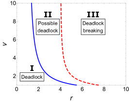
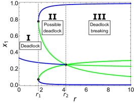
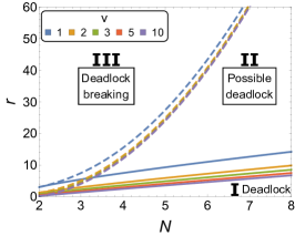
Figure 1: Dynamics of the complete decision system of Equation (3) for the symmetric case $\kappa=1$ (i.e., $v_{1}=v_{2}=v_{3}=v$). Panel 1 shows the stability diagram as a function of the parameter $r$ and the quality $v$ for $N=3$ options. The two curves represents the two bifurcations $r_{1}$ (blue solid) and $r_{2}$ (red dashed) of Equations (4). There are three possible system phases: (I) decision-deadlock, (II) coexistence of decision deadlock and stable solutions for any option, and (III) decision for any option. Panel 1 shows the bifurcation diagram for $N=3$ and $v=5$ as a function of the parameter $r$. This illustrates the three system phases when varying the control parameter $r$. Note that, due to the 2D visualisation, some equilibria overlap and thus the bottom branches in panel 1 correspond to the two overlapping equilibria for the options $x_{2}$ and $x_{3}$. Panel 1 shows a stability diagram that visualises the dependence of the bifurcation points $r_{1}$ (solid lines) and $r_{2}$ (dashed lines) as a function of $N$ for varying $v\in\{1,2,3,5,10\}$, and reports the same three system phases.

We start by analysing the symmetric case of $N$ equal-quality options (i.e. $\kappa=1$). The simplicity of the reduced system (Equation (13)) allows us to determine the existence of two bifurcation points which are determined by the parameters $r$, $v$ and $N$, and we show the bifurcation conditions in terms of the control parameter $r$ as:

$$r_{1}=f_{1}(v,N),\qquad r_{2}=f_{2}(v,N)\,.$$ (4)

In Appendix D, we report the complete equations for (4) as functions of $(v,N)$ (see Equation (21)) or, more generally, of $(\gamma$,$\alpha$,$\rho,\beta)$ (see Equation (19)). In Figure 1, we show the stability diagram of the system (3) in the parameter space $(r,v)$, for $N=3$. When the pair $(r,v)$ is in area I, the system cannot break the decision deadlock but remains in an undecided state with an equal number of bees in each of the three committed populations. This result can be also seen in Figure 1, where we display the bifurcation diagram for the specific case $v=5$. Here, low values of $r$ correspond to a single stable equilibrium representing the decision deadlock. Increasing the signalling ratio, the system undergoes a saddle node bifurcation when $r=r_{1}$ in Figure 1, at which point a stable solution for each option appears and the selection by the swarm of any of the $N$ equally-best quality options is a feasible solution. However, for $(r,v)$ in area II of Figure 1, the decision-deadlock remains a stable solution and only through a sufficient bias towards one of the options the system converges towards a decision. This system phase can be visualised in the bifurcation diagram of Figure 1 and in the phase portrait of Figure 2: The system escapes from the decision-deadlock attraction basin if noise leads the population to jump into a neighbouring basin corresponding to a unique choice.

Figure 2: Phase portraits of the complete system (3) for $N=3$ options in the symmetric case $\kappa=1$ (i.e., $v_{1}=v_{2}=v_{3}=v=5$). Blue dots represent stable equilibria, and green dots represent unstable saddle points. Saddle manifolds are shown as red (repulsive) and blue (attracting) lines. Panel 2 shows the system in a decision deadlock phase (i.e., phase I of Figure 1, $r=1$), in fact, there is only one stable solution with all the three committed population with equal size. Panel 2 shows the coexistence of the decision deadlock and the decision for any option (phase II, $r=3$). Panel 2 shows the system for high values of $r$ in which the decision deadlock solution is an unstable saddle point, and therefore the only stable solutions are the decision for any option (phase III, $r=10$). The same phase portrait from another perspective is shown in panel (d) where a set of trajectories (red lines) are shown. Looking at panel (d), the central unstable saddle node is unstable on the displayed plane while is stable (i.e., attracting) on the direction orthogonal to the field of view of the plot (d) (i.e., the attraction manifold is the line $x_{1}=x_{2}=x_{3}$). The system does not possess any periodic attractors.

The system undergoes a second bifurcation at $r=r_{2}$ in Figure 1, that changes the stability of the decision-deadlock from stable ($r<r_{2}$) to partially unstable (saddle, $r>r_{2}$). Therefore, for sufficiently high values of the signalling ratio (area III in Figure 1), the unique possible outcome is the decision for any of the equally best quality options. The central solution of indecision remains stable (i.e., attracting) with respect to only one manifold, i.e., the line for equal-size committed populations, while it is unstable with respect to the other directions (see the phase portraits of Figures 2-2 and the video in the supplemental material sup ). Instead, the unstable saddle points that surround the central solution have opposite attraction/repulsion manifolds. For this reason, several unstable equilibria can be near to each other, as in Figure 1.

The analysis of the system with three options reveals three system phases as a consequence of the two bifurcations determined by $f_{1}$ and $f_{2}$ (Equation (4)). Increasing the number of options, the number of system phases increases. In particular, for every other $N$, at odd values (i.e., $N\in\{5,7,9,\dots\}$), a new bifurcation point between $r_{1}$ and $r_{2}$ appears. In Figure 10, we report the bifurcation diagrams for $v=5$ and $N\in\{4,5,6,7\}$. Despite the system phase increase, the main dynamics for any $N>2$ can be described by the three macro-phases described above: (I) decision-deadlock only, (II) coexistence of decision-deadlock and decision, and (III) decision only. In fact, the additional equilibria that appear for odd $N$ are all unstable saddle solutions (with orthogonal attraction/repulsion directions with each other) which do not change the stability of other solutions. Therefore, we focus our study on the bifurcations defined by Equations (4) (i.e., Eq. (21)) which determine the main phase transitions.

Figure 1 shows the relationship between the bifurcation points $r_{1}$ and $r_{2}$, the options’s quality $v$ and the number of options $N$. The effect of $v$ on $r_{1}$ and $r_{2}$ remains similar to that seen in Figure 1, i.e., the bifurcation points vary as a function of $v$ when $v$ is low, while they are almost independent of $v$ when it is large. More precisely, the influence of the quality magnitude $v$ on the system dynamics decreases quadratically with $v$ (see Equation (21)). The number of options, $N$, influences differently the two bifurcation points. While $r_{1}$ grows quasi-linearly with $N$, instead $r_{2}$ grows quadratically with $N$. Therefore, in the symmetric case, the number of options that the swarm considers plays a fundamental role in the decision dynamics. In fact, too many options preclude the possibility of breaking the decision-deadlock and selecting one of the equally-best options. This result suggests a limit on the maximum number of equal options that can be concurrently evaluated by the modelled decision-maker.

III.2 Asymmetric case

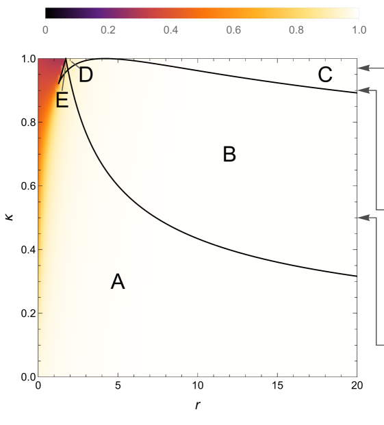
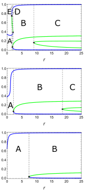
Figure 3: Dynamics of the complete decision system of Equations (3) for $N=3$ options for the asymmetric case ($\kappa<1$) and superior option’s quality $v=5$. The left panel shows the stability diagram as a function of the parameter $r$ and the ratio between qualities $\kappa$. The parameter space is divided in five different areas (see Figure 8 to see a representative 3D phase portrait for each area). In area A, the system has a unique solution corresponding to selection of the best option; in areas B and C, the system may select any of the possible options; in areas D and E the system may end in a decision deadlock. The underlying density map show the population size of the stable solution for the best option. For low values of $r$ and similar options (top-left corner), this population is relatively small and may be not enough to reach a quorum threshold. The right panels show three bifurcation diagrams as a function of the parameter $r$ for $\kappa\in\{0.5,0.9,0.97\}$. Note that, due to the 2D visualisation, some equilibria overlap and thus the bottom branches of the bifurcation diagrams correspond to two overlapping equilibria for selection of options $x_{2}$ and $x_{3}$.

We next analyse the system dynamics in the asymmetric best-of-N case where option 1 is superior to the other $N-1$ same-quality, inferior options $i$ (with $i\in\{2,\dots,N\}$). Figure 3 shows the stability diagram for $N=3$ options in the paremeter space $r,\kappa$. The results show that low values of $r$ allow the system to have a unique solution, (area A in the left panel of Figure 3). This is especially true when the difference between the options is larger (i.e., low values of $\kappa$). However, such stable solutions may not correspond to a clear-cut decision, as the population fraction committed to the best alternative may be too low to reach a decision threshold, as indicated by the underlying density map in Figure 3: if $r$ is small and $\kappa$ sufficiently high, only about half of the population will be committed to the best option. Hence, a sufficiently high value of $r$ is required for the implementation of a collective decision. For larger values of $r$, the system undergoes various bifurcations leading to $N$ stable solutions corresponding to the selection of each available option (areas B and C of the left panel in Figure 3). Therefore, there is the possibility that an inferior option gets selected. For high values of $\kappa$, two additional areas appear, labelled D and E in Figure 3. These areas correspond to the co-existence of an undecided state together with a decision state for the superior and/or the inferior options, similarly to area II in Figure 1. The bifurcation diagrams in the right panels show the effects of $r$ for fixed values of $\kappa$. When the best option has double quality than the inferior options (i.e., $\kappa=0.5$, see the bottom-right panel), a low value of $r$ guarantees selection of the best option, whereas a sufficiently high $r$ may result in incorrect decisions by selecting any of the inferior options (which are considerably worse than the best one). As the inferior options become comparable to the superior one, the range of values of $r$ in which there exists a single stable equilibrium in favour of the best options gets reduced (see the middle-right panel for $\kappa=0.9$ in Figure 3), up to the point that there is no value of $r$ in which the choice of the superior option is the unique solution (see the top-right panel for $\kappa=0.97$ in Figure 3). In this case, however, there is little difference in quality between the superior and inferior options, and the system dynamics are similar to the symmetric case in which it is most valuable to break a decision deadlock, hence to choose a sufficiently high value of $r$.

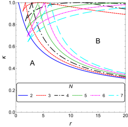
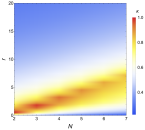
Figure 4: 4 Stability diagram for best option quality $v=5$ in the parameter space $r,\,\kappa$ for varying number of options $N\in\{2,\dots,7\}$. For each option, the system has five possible phases that are consistent with the phases described in caption the of Figure 3. Here we label only areas A (monostability) and B (multistability) to facilitate readability. 4 Maximum value of $\kappa$ as a function of $N\in\{2,\dots,7\}$ and $r\in(0,20]$ for which the system has a unique attractor for the selection of the best quality option, defined as the best option attracting commitment from at least 75% of the total decision-making population.

The dynamics observed for $N=3$ options are consistent in the case of $N>3$. Figure 4 shows the stability diagram for varying number of options $N\in\{2,\dots,7\}$ (see also Figure 9). It is possible to note that areas D and E get larger as $N$ increases, leading to a larger range of values in which one or more stable decision states coexist with a stable undecided state, up to the point that area C disappears for $N\geq 5$. This means that, as the number of inferior options increases, the probability of making a wrong decision increases as well, especially for high values of $\kappa$. To minimise the probability of wrong decisions, the value of $r$ should be maintained as small as possible, but still high enough to ensure that a decision is taken (i.e., with a sufficiently large population committed to one option, see the density map in Figure 9). Finally, in Figure 4 we show how the ability to solve hard decision problems varies with $r$ and $N$. To this end, for each point in the space $r,N$, we show the highest value of $\kappa$ for which there exists a unique attractor for the superior option corresponding to at least 75% of the population committed (i.e., $x_{1}\geq 0.75$). Figure 4 demonstrates an approximately linear relationship between $r$ and $N$ for a given value of $\kappa$.

IV Discussion

We have analysed a model of consensus decision-making which exhibits useful value-sensitive properties that have previously been described for binary decisions Pais et al. (2013), but generalises these to decisions over three or more options. In order to preserve these properties the single control parameter in the original model of Pais et al. (2013), the rate of cross-inhibition between decision populations, is replaced by a parameter describing the relative frequencies with which individual group members engage in independent discovery and abandonment behaviours, compared to positive and negative-feedback signalling behaviours. This new control parameter is biologically meaningful and experimentally measurable, so should be of interest for further empirical studies of house-hunting honeybee swarms.

Previous work has investigated the role of signalling in collective decision making in a somewhat different framework. Galla Galla (2010) has analysed a model of house-hunting honeybees List et al. (2009) where the cross-inhibition mechanism was not included. In this model, increasing signalling (referred to as interdependence) allows the swarm to select the best quality option more reliably. The interdependence parameter modulates the strength of positive feedback; the higher the interdependence is, the more a bee is influenced by other bees’ opinion in determining a change of commitment. There are similarities and differences between the meaning of the interdependence parameter and the signalling ratio $r$ that is introduced in this paper. Similarly to Galla (2010); List et al. (2009), increasing the value of the ratio $r$ corresponds to an increase in the signalling behaviour but, in contrast to previous studies, $r$ is a weighting factor of both positive and the negative feedback. However, note that positive and negative feedback are not necessarily equal in our model, as these mechanisms are also modulated by the option’s quality. In agreement with Galla (2010); List et al. (2009), our results underline the importance of interactions among honeybees in the nest-site selection process. However, given the different meanings of the control parameters, we find that increased signalling behaviour helps to break decision deadlocks (in case of equal alternatives) but too high signalling might reduce the decision accuracy when the decision has to be made among different quality options.

We also note some similarities between our results and the bifurcation analysis of a model of the collective decision making process in foraging ants Lasius niger Nicolis and Deneubourg (1999). This model describes the temporal evolution of the pheromone concentration along $N$ alternative trails, each of which leads to a different food source. The bifurcation parameter in the analysis is an aggregate variable composed of the total population size, the options’ qualities and the pheromone evaporation rate. Not all of these components are under the direct control of the decision maker, and thus cannot be varied during the decision process. In contrast, the control parameter in our analysis, the signalling ratio $r$, can be modulated in a decentralised way by the individual bees. Comparing the bifurcation diagrams for deadlock breaking of Fig. 3(a) in Nicolis and Deneubourg (1999) with Fig. 10, the two models present similar dynamics. The authors also present a hysteresis loop as a function of relative food source quality (Fig. 4 in Nicolis and Deneubourg (1999)), which is similar to that found as a function of relative nest-site quality in Pais et al. (2013) (Fig. 5). Collective foraging over multiple food sources is a fundamentally different problem to nest-site selection, with exploitation of multiple sources frequently preferred in the former whereas convergence on a single option is required in the latter Marshall et al. (2009). Nevertheless it could be interesting to make further comparisons of the dynamics of the model presented here and other nonlinear dynamical models exhibiting qualitatively similar behaviour.

A crucial point in our model is that honeybees need to interact at a rate that is high enough to break decision deadlock in the case of equal options, in addition to the influence of nest-site qualities. This follows from our analysis of the symmetric case (Section III.1), where we observed that high signalling ratio $r$ allows the system to break the decision deadlock and to select any of the equally best options. However, the analysis of the asymmetric case (Section III.2) revealed that a frequent signalling behaviour may have a negative effect on the decision accuracy, and low $r$ values should be preferred to have a systematic choice of the best available option. These results suggest that a sensible strategy may be to increase $r$ through time. An organism may start the decision process applying a conservative strategy which reduces unnecessary costs of frequent signalling behaviour and that, at the same time, allows quickly and accurately to select the best option if it is uniquely the best. Otherwise, in the case of a decision deadlock (due to multiple options having similar qualities), the system may increase its signalling behaviour in order to break symmetry and converge towards the selection of the option with the highest quality. This strategy is reminiscent of the suggested strategy of increasing cross-inhibition over time to spontaneously break deadlocks in binary decisions Pais et al. (2013). Further theoretical evidence supporting such a strategy comes from the bifurcation diagrams presented in the middle- and top-right panels in Figure 3, corresponding to asymmetric case with $N=3$ similar options, with $\kappa=0.9$ and $\kappa=0.97$, respectively (see also Figure 11 for further bifurcation diagrams with $N\in\{4,5,6,7\}$). In these cases, an incremental increase in $r$ would allow the system to converge accurately towards the best option. In contrast, immediately starting the decision process with a high value of $r$ might decrease the decision accuracy. For instance, in Figure 3 (right-center), starting with low values of $r$ (i.e., $r<2.1$) would bring the system to the stable attractor (blue line) with less than half of the population committed to the best option. A gradual increase of $r$ lets the process follow the (blue, stable) solution line which leads to the selection of option $1$. On the other hand, a process that starts from a totally uncommitted state with a value of $r>2.1$ may end in the basin of attraction corresponding to selection of an inferior option, as a consequence of stochasticity of the decision process. Such a strategy could easily be implemented in a decentralised manner by individual group members slowly increasing their propensity to engage in signalling behaviours over time; such a direction of change, from individual discovery to signalling behaviour, is also consistent with the general requirement of a decision-maker to gather information about available options, but then to begin restricting consideration to these rather than investing time and resources in the discovery of further alternatives. Theorists and empiricists have previously concluded that honeybee swarms achieve consensus through the expiration of dissent Seeley (2003), which occurs as bees apparently exhibit a spontaneous linear decrease in number of waggle runs for a nest over time Seeley and Buhrman (1999). However, the discovery of stop-signalling in swarms requires that this hypothesis be re-evaluated, since increasing contact with stop-signalling bees over time will also decrease expected waggle dance duration Seeley et al. (2012). Field observations report that recruitment decreases over time in easy decision problems while it increases overall in difficult problems (e.g. five equal-quality nests) Seeley et al. (2006). Further theoretical work with our model would reveal whether it is capable of explaining these empirically-observed patterns.

Our analyses also suggest an optimal stable signalling ratio that the decision-making system might converge to. While the level of signalling required to break deadlock between $N$ equal options increases quadratically with $N$ (Figure 1), the level of signalling that optimises the discriminatory ability of the swarm in best-of-N scenarios increases only linearly (Figure 4). Optimising best-of-N decisions therefore seems at odds with optimising equal alternatives scenarios. However in natural environments the probability of encountering $N$ (approximately) equal quality nest options will decrease rapidly with $N$. On the other hand the best-of-N scenario here, while still less than completely realistic, should still provide a better approximation to the naturalistic decision problems typically encountered by honeybee swarms. Our analysis shows that the level of signalling that swarms converge to may be tuned appropriately by evolution according to typical ecological conditions, namely the number of potentially suitable nest sites that are typically available within flight distance of the swarm. Swarms of the European honeybee Apis mellifera are able to solve the best-of-N problem with one superior option and four inferior options Seeley and Buhrman (2001), presumably reflecting the typical availability of potential nest sites in their ancestral environment.

While our model is inspired by nest-site selection in honeybee swarms, we feel its relevance is potentially much greater. For example, as mentioned in the introduction, decision-making in microbial populations may share similarities with decisions by social insect groups Ross-Gillespie and Kümmerli (2014). In addition cross-inhibitory signalling is a typical motif in intra-cellular decisions over, for example, cell fate Nené et al. (2012), and single cells can exhibit decision behaviour similar to Weber’s law Ferrell (2009); Goentoro et al. (2009). Weber’s law describes how the ability to perceive the difference between two stimuli varies with the magnitude of those stimuli, and may have adaptive benefits Akre and Johnsen (2014). Several authors have also noted similarities between collective decision-making and organisation of neural decision circuits, where inhibitory connections between evidence pathways are also typical Couzin (2007); Marshall and Franks (2009); Couzin (2009); Passino et al. (2007); Marshall et al. (2009). Similarly, neural circuits following the winner-take-all principle have dynamics regulated by the interplay of excitatory and inhibitory signals and present interesting analogies to the present model Douglas et al. (1995); Rutishauser et al. (2011). Since organisms at all levels of biological complexity must solve very similar statistical decision problems that relate to fitness in very similar ways, we feel there is definite merit in continuing to pursue the analogies between collective decision-making models such as that presented here, and models developed in molecular biology and in neuroscience. Finally, we suggest that the simplicity of the model presented here and its adaptive decision-making characteristics might inform the design of artificial decentralised decision-making systems, particularly in collective robotics (e.g. Leonard (2014); Reina et al. (2015a, b, 2016)) and in cognitive radio networks (e.g. Trianni et al. (2016)).

V Acknowledgments

This work was funded by the European Research Council (ERC) under the European Union’s Horizon 2020 research and innovation programme (grant agreement number 647704). Vito Trianni acknowledges support by the European Commission through the Marie Skłodowska-Curie Career Integration Grant “DICE, Distributed Cognition Engineering” (Project ID: 631297).

Appendices

The appendixes are organised in five sections. In Appendix A, we present the complete model in all the parameterisations discussed in the article (from the most general to the most specific). Then, we report the reduced model in a similar set of parameterisations. In Appendix B, we show that the parameterisation used in the literature Pais et al. (2013) cannot break the decision deadlock in the symmetric case when the number of options is larger than two. In Appendix C, we study the dynamics of the system in the selected parameterisation for the binary case, i.e., $N=2$. In Appendix D, we report the formulas of the two main bifurcation points for the symmetric case. This formula is particularly significant because it is valid for any number of options. In Appendix E, we report additional results on the system dynamics: we report additional analysis performed on the system deciding between three options, and we show that the results for $N=3$ options are qualitatively similar for $N>3$.

Appendix A Complete model and reduced model

The general model for $N$ options is:

$$\left\{\begin{aligned} \frac{dx_{i}}{dt}&=\gamma_{i}\,x_{u}-\alpha_{i}\,x_{i}+\rho_{i}\,x_{u}\,x_{i}-\sum_{j=1}^{N}\,x_{j}\,\beta_{ji}\,x_{i}\,,\qquad i\in\{1,\,\dots\,,\,N\}\,,\\ x_{u}&=1-\sum_{i=1}^{N}x_{i}\end{aligned}\right.$$ (5)

where $x_{i}$ represents the subpopulation committed to option $i$ and $x_{u}$ the uncommitted subpopulation. $\gamma_{i}$ represents the discovery rate for option $i$, $\alpha_{i}$ the abandonment rate for option $i$, $\rho_{i}$ the recruitment rate for option $i$ and $\beta_{ji}$ the cross-inhibition from subpopulation $j$ to subpopulation $i$.

We introduce a first parameterisation as:

$$\gamma_{i}=k\,v_{i}\qquad\alpha_{i}=k\,v_{i}^{-1}\qquad\rho_{i}=h\,v_{i}\qquad\beta_{ii}=0\qquad\beta_{ij}=\beta$$ (6)

with $i\neq j$. By applying Equation (6) in (5), we obtain:

$$\left\{\begin{aligned} \frac{dx_{i}}{d\tau}&=v_{i}\,x_{u}-\frac{x_{i}}{v_{i}}+r\,v_{i}\,x_{u}\,x_{i}-\sum_{j=1,\,j\neq i}^{N}\,x_{i}\,\beta\,x_{j}\,,\qquad i\in\{1,\,\dots\,,\,N\}\,,\\ x_{u}&=1-\sum_{i=1}^{N}x_{i}\end{aligned}\right.$$ (7)

where $r=h/k$ is the ratio of interaction over spontaneous transitions, and $\tau=k\,t$ is the dimensionless time. The parameterisation of Equation (6) is a generalisation of the one proposed in the literature Pais et al. (2013), since, using $r=1$, the system (5) reduces to the old one, and thus displays the same dynamics.

This intermediate steps allows us to visualise that for $r\leq 1$ there is no value of $\beta$ that allows to break the decision deadlock in the case of $N>2$ same-quality options (see Figure 5). This result motivates the change of parameterisation with respect to previous work Pais et al. (2013). Additional analyses that confirm the presence of the decision deadlock for values of $r=1$ are provided in Appendix B.

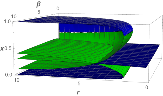
Figure 5: Bifurcation diagram in 3D of the system (7) with $N=3$ equal-quality options (i.e., $v_{1}=v_{2}=v_{3}=v$) as a function of $r=h/k\in(0,10]$ and $\beta\in(0,10]$. The vertical axis shows $x\in[0,1]$, which represents the proportion of bees committed to one of the three identical options. Blue surfaces represent stable equilibria, while green surfaces are unstable equilibria. We can see that for $r=1$, the decision deadlock is stable for any tested values of $\beta$. See Section B for a formal proof of the decision deadlock for $r=1$ and $N=3$.

We modify the parameterisation of Equation (6) by linking the signalling behaviours (recruitment and cross-inhibition) with the same value. The modified parameterisation is:

$$\gamma_{i}=k\,v_{i}\qquad\alpha_{i}=k\,v_{i}^{-1}\qquad\rho_{i}=h\,v_{i}\qquad\beta_{ij}=h\,v_{i}$$ (8)

and by applying Equation (8) in (5), we obtain:

$$\left\{\begin{aligned} \frac{dx_{i}}{d\tau}&=v_{i}\,x_{u}-\frac{x_{i}}{v_{i}}+r\,v_{i}\,x_{i}\left[x_{u}-\sum_{j\neq i}\,\kappa_{ji}\,x_{j}\right]\,,\qquad i,\,j=1,\,...\,,\,N\,,\\ x_{u}&=1-\sum_{i=1}^{N}x_{i}\end{aligned}\right.$$ (9)

where $\kappa_{ij}=v_{i}/v_{j}$ the ratio between options’s values (and $\tau=k\,t$, again, is the dimensionless time).

The reduced model. In this study, we investigate the scenario in which there is one superior option and $N-1$ equal-quality inferior options. Assuming that the best option is the option $1$, the Equation (5) can be simplified through the following variable change:

$$x_{A}=x_{1}\qquad x_{B}=\sum_{i=2}^{N}x_{i},\qquad\lambda_{1}=\lambda_{A}\qquad\lambda_{i}=\lambda_{B}\qquad\lambda\in\{\gamma,\alpha,\rho,\beta\}\qquad i\in\{2,\dots,N\}\,.$$ (10)

By applying Equation (10) to the complete system (5), we obtain:

$$\left\{\begin{aligned} \frac{dx_{A}}{dt}&=\gamma_{A}\,x_{u}-\alpha_{A}\,x_{A}+\rho_{A}\,x_{A}\,x_{u}-\beta_{B}\,x_{A}\,x_{B}\,,\\ \frac{dx_{B}}{dt}&=(N-1)\,\gamma_{B}\,x_{u}-\alpha_{B}\,x_{B}+\rho_{B}\,x_{B}\,x_{u}-\frac{N-2}{N-1}\,\beta_{B}\,x_{B}^{2}-x_{A}\,x_{B}\beta_{A}\,,\\ x_{u}&=1-x_{A}-x_{B}\,,\end{aligned}\right.$$ (11)

Similarly, Equation (9) can be simplified through the following variable change:

$$x_{A}=x_{1}\qquad x_{B}=\sum_{i=2}^{N}x_{i},\qquad v=v_{1},\qquad\kappa=\frac{v_{1}}{v_{i}}\qquad v_{i}=\kappa\,v,\qquad i\in\{2,\dots,N\}\,.$$ (12)

By applying Equation (12) to the complete system (9), we obtain:

$$\left\{\begin{aligned} \frac{dx_{A}}{d\tau}&=v\,x_{u}-\frac{x_{A}}{v}+r\,v\,x_{A}\left[x_{u}-\kappa\,x_{B}\right]\,,\\ \frac{dx_{B}}{d\tau}&=(N-1)\,\kappa\,v\,x_{u}-\frac{x_{B}}{\kappa\,v}+r\,v\,x_{B}\left[\kappa\,\left(x_{u}-\frac{N-2}{N-1}\,x_{B}\right)-x_{A}\right]\,,\\ x_{u}&=1-x_{A}-x_{B}\,,\end{aligned}\right.$$ (13)

Appendix B Need for a novel parameterisation: Decision deadlock for $N=3$

In this appendix, we show that the model of Equation (7) with $r=1$ and $N=3$ cannot break the decision deadlock for any values of $\beta\geq 0$.

To prove this, we start from the reduced system given in Equation (11) (we could also use the full three-dimensional system but due to the higher number of equilibria this is more difficult). Note that Equation (11) describes the reduced system before value-sensitivity is introduced. In this form it is also equivalent to the case $r=1$.

We assume that $\alpha_{A}=\alpha_{B}=\alpha$, $\beta_{A}=\beta_{B}=\beta$, $\gamma_{A}=\gamma_{B}=\gamma$, and $\rho_{A}=\rho_{B}=\rho$. If we calculate the equilibria we find that there are up to four different points. One is always negative and unstable. Depending on the other three stationary states (the symmetric solution, and two more) and their stability, we determine if the decision maker ends up in decision-deadlock, or not.

Investigating the existence of the equilibrium points we can write down a generalised condition determining the existence of the two non-symmetric equilibrium solutions that evolve at the bifurcation point (cf. Seeley et al. (2012); Pais et al. (2013)). This reads:

$$\begin{aligned} (-\alpha\beta+&2\beta\gamma+\alpha\beta N-3\beta\gamma N+\beta\gamma N^{2}+\beta\rho-\beta N\rho)^{2}\\ &-4(\alpha\gamma-2\alpha\gamma N+\alpha\gamma N^{2})(-2\beta^{2}+\beta^{2}N-\beta\rho+\beta N\rho)=0\,\,.\end{aligned}$$ (14)

We may resolve this equation with respect to $\beta$.

(1) If we let $N=2$ we obtain

$$\begin{aligned} \beta=\frac{4\alpha\gamma\rho}{(\rho-\alpha)^{2}}\,\,,\end{aligned}$$ (15)

as in the original model in Seeley et al. (2012).

(2) If we now introduce value-sensitivity, i.e. $v_{1}=v_{2}=v$ ($2$ equal options), and let $N=2$, $\rho=v$, $\gamma=v$, $\alpha=1/v$ we get:

$$\begin{aligned} \beta=\frac{4v^{3}}{(1-v^{2})^{2}}\,\,,\end{aligned}$$ (16)

which coincides with the result reported in Pais et al. (2013).

(3) If we let $N=3$ (and accordingly $v_{1}=v_{2}=v_{3}=v$ ($3$ equal options)), $\rho=v$, $\gamma=v$, $\alpha=1/v$, which is the extension from $2$ options (see model in Pais et al. (2013)) to $3$ options we obtain for $v>1/2$:

$$\begin{aligned} \frac{8v^{3}}{1-4v^{2}}<\beta<0\,\,.\end{aligned}$$ (17)

In Eqs. (15) - (17) we gave the condition for the existence of the two stationary points which might be reached by the decision-maker in addition to the symmetric solution. These are related to pitchfork ($N=2$) or limit point ($N=3$) bifurcations. If the parameter $\beta$ does not range in these intervals only the symmetric equilibrium is real and positive, which is the condition for biological meaningful states. This symmetric equilibrium is also stable. In particular, Eq. (17) shows that $\beta$ needs to be negative to make the stationary states in question occur. As, on the other hand, $\beta$ needs to be positive in order to describe cross-inhibition, this case has to be excluded and hence we have shown that the parametrisation introduced in Pais et al. (2013) cannot describe decision-deadlock breaking for $3$ options, as only one stable equilibrium exists (the symmetric solution) for $r=1$ and all $\beta\geq 0$.

Also note that the quality values associated with the available options should be $v\geq 1$. Otherwise, some of the available states may take negative values, which is not a biologically relevant solution. This applies to all the parametrisations mentioned above.

Appendix C Effects of the novel parameterisation for $N=2$

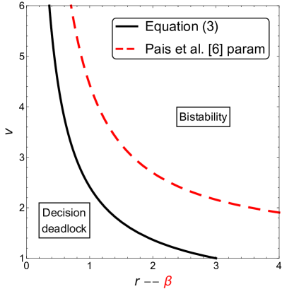
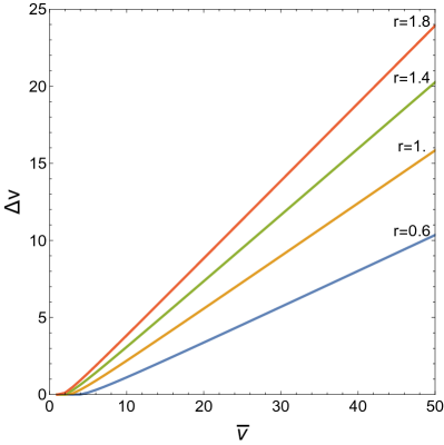
Figure 6: 6 Comparison of the stability diagrams in the binary and symmetric case (i.e., $N=2$ and $v_{1}=v_{2}=v$) of the newly proposed parameterisation (Eq. (3)) and the previous work Pais et al. (2013). The bifurcation line that determines the two system phases is qualitatively similar, but the bifurcation parameter is different: In the previous work it is the cross-inhibition signal $\beta$, here it is the interaction ratio $r$. 6 Stability diagram of the system (3) as a function of the average quality $\bar{v}=(v_{1}+v_{2})/2$ and the quality difference $\Delta v=|v_{1}-v_{2}|$ for varying $r\in\{0.6,1,1.4,1.8\}$, in the binary decision case. The lines show the relationship between the minimum quality difference to have the system with an unique attractor for the best option and the quality mean. This relationship resembles the Weber’s law observed in psychological studies, with $r$ determining the coefficient. The results are similar to the ones obtained in Pais et al. (2013), but using a different coefficient (in the previous work the coefficient was the cross-inhibition, $\beta$).

We study the dynamics of the systems (3) that uses a novel parameterisation with respect to previous work Seeley et al. (2012); Pais et al. (2013). We test if, in the binary decision case (i.e., $N=2$), the system dynamics are comparable to the dynamics reported in the literature.

Figure 6 shows a comparison of the stability diagrams for the symmetric case of two options with equal value $v$. The system dynamics are qualitatively similar but the bifurcation parameter is different. In Pais et al., the bifurcation is determined by the cross-inhibition $\beta$, while in our parameterisation it is determined by the ratio of interaction/spontaneous transitions $r=h/k$.

Additionally, Pais et al. Pais et al. (2013) showed that the cross-inhibition determines the minimum difference necessary to discriminate between two similar quality options in a manner similar to the Weber’s law. We obtain similar results but using a different parameter. In Figure 6 we show that the interaction ratio $r$ determines the just noticeable difference.

Appendix D Bifurcations in the symmetric case

In case of $N$ equal-quality options, hereafter called the symmetric case, the values of every transition rate are the same for both equation $A$ and $B$, i.e., $\gamma_{A}=\gamma_{B}=\gamma$, $\alpha_{A}=\alpha_{B}=\alpha$, $\rho_{A}=\rho_{B}=\rho$ and $\beta_{A}=\beta_{B}=\beta$. The reduced system of Equation (11) becomes:

$$\left\{\begin{array}[]{ll}\dot{x}_{A}&=\gamma x_{U}-\alpha x_{A}+\rho x_{U}x_{A}-\beta x_{A}x_{B}\\ \dot{x}_{B}&=(N-1)\gamma x_{U}-\alpha x_{B}+\rho_{B}x_{U}x_{B}-\beta x_{B}(x_{A}+\frac{N-1}{N-2}x_{B})\\ x_{U}&=1-x_{A}-x_{B}\\ \end{array}\right.,$$ (18)

System (18) undergoes two bifurcations. The simplicity of Equation (18) allows us to analytically derive the formula of the two bifurcation points:

$$\begin{aligned} \rho_{1}&=\frac{\alpha(2\gamma(N-1)+\sigma)+2\sqrt{\alpha}\sqrt{\gamma}\sqrt{\alpha(N-1)+\sigma(N-2)}\sqrt{\gamma(N-1)+\sigma}+\gamma\sigma(N-2)}{\sigma}\\ \rho_{2}&=\frac{\alpha\left(\sqrt{\gamma}N\sqrt{\gamma N^{2}+4\sigma}+\gamma N^{2}+2\sigma\right)+\sqrt{\gamma}\sigma(N-2)\left(\sqrt{\gamma N^{2}+4\sigma}+\sqrt{\gamma}N\right)}{2\sigma}\quad.\end{aligned}$$ (19)

In the symmetric case, the system (3) becomes:

$$\left\{\begin{aligned} \frac{dx_{A}}{d\tau}&=v\,x_{u}-\frac{x_{A}}{v}+r\,v\,x_{A}\left[x_{u}-x_{B}\right]\,,\\ \frac{dx_{B}}{d\tau}&=(N-1)\,v\,x_{u}-\frac{x_{B}}{v}+r\,v\,x_{B}\left[x_{u}-\frac{N-2}{N-1}\,x_{B}-x_{A}\right]\,,\\ x_{u}&=1-x_{A}-x_{B}\,,\end{aligned}\right.$$ (20)

and undergoes two bifurcations at:

$$\begin{aligned} r_{1}&=\frac{1}{v^{2}}-2+N+\frac{2\sqrt{2N-3}}{v}\\ r_{2}&=(N-3)N+2+\frac{1}{v^{2}}+\frac{N-1}{v}\sqrt{(4+v^{2}(N-2)^{2})}\quad.\end{aligned}$$ (21)

Note, that here the bifurcation points are expressed as a function of $N$, $r$ and $v$.

Appendix E System dynamics

Best of three.

Figure 7 shows the time dependent solutions of the system with $N=3$ options for varying values of $\kappa\in\{0.25,0.5,0.75\}$. The plot shows the dynamics of the population committed to the best quality option $x_{1}$. For decreasing values of $\kappa$ the system converges faster to the stable equilibrium $x_{1}=1$. The system parameters are in a plausible range for the honeybee nest-site selection process leading to convergence times that are comparable to field experiments, interpreting $t$ in hour units Seeley and Buhrman (2001).

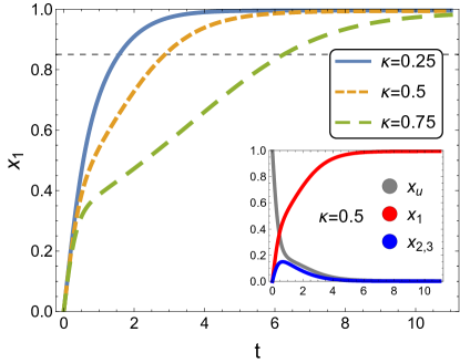
Figure 7: Time dependent solutions of the system of Equations (1)-(2) for $N=3$ options, spontaneous transitions strength $k=0.1$, interaction transitions strength $h=0.3$, best option quality $v=10$, and varying inferior alternatives’ quality as $\kappa\in\{0.25,0.5,0.75\}$. The main plot displays the dynamics of the population committed to the best quality option $x_{1}$; the inset shows the dynamics of all populations for $\kappa=0.5$, note that the populations committed for the inferior alternatives, $x_{2}$ and $x_{3}$, have overlaying trajectories. The horizontal dashed line shows an example quorum threshold Seeley and Visscher (2004).

In Figure 3, we identify five system phases (labelled as A, B, C, D and E) for the asymmetric case and $N=3$. In Figure 8, we report a representant 3D phase portrait of the system (3) for each of the five system phases.

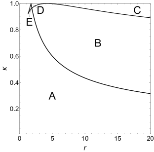
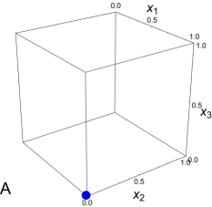
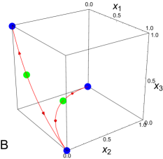
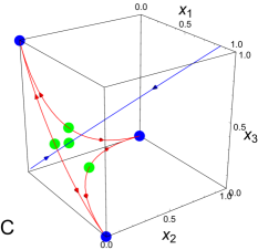
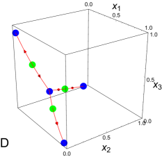
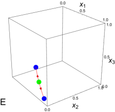
Figure 8: Dynamics of the system (3) in the case of $N=3$ options. In the top-left panel, we report the stability diagram in the parameter space $r$, $\kappa$. The plot shows that there are five possible system phases, labelled with letter from A to E. The other panels show a representative 3D phase portrait for each phase. The letter in the bottom-right of each phase portrait indicates which phase they represent.

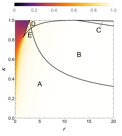
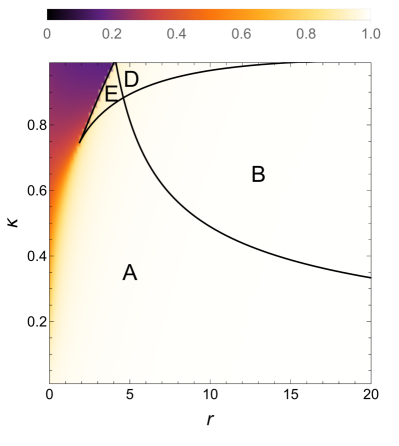
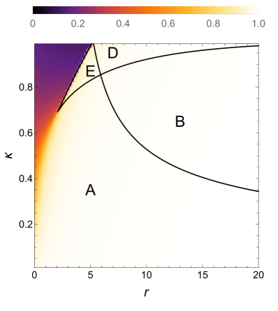
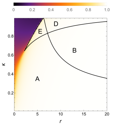
Figure 9: Stability diagrams for $v=5$ and $N\in\{4,5,6,7\}$, in panel 9, 9, 9, and 9, respectively. The area A indicates the systems phase with a single attractor in favor of the best option. Having an unique solution, in this area the system never converges for the selection of inferior options. The underlying density map shows the population size of the stable solution for the best option. In the dark area the population for the best option is not sufficient to reach a quorum to take a decision. For an increasing number of options, the dark area increases and low values of $r$ are not sufficient anymore to allow the swarm to take a decision for similar options (high $\kappa$). However, for sufficiently large values of $r$, the area A shifts towards higher values of $\kappa$. This effect is also shown in Figure 4 of the main text.

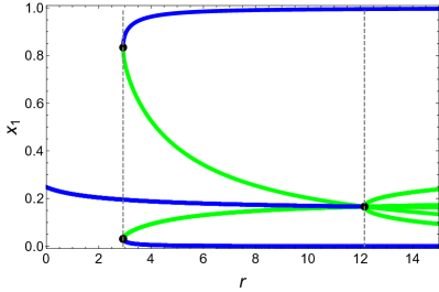
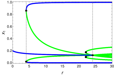
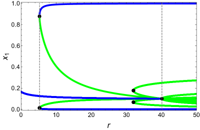
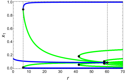
Figure 10: Bifurcation diagrams of the complete system (Equation (3)) in the symmetric case ($v=5$) for number of options $N=4$ in panel 10, $N=5$ in panel 10, $N=6$ in panel 10, and $N=7$ in panel 10. Blue curves represent stable equilibria and green lines unstable saddle points. The vertical dashed lines are the bifurcation point predicted by the reduced system (Equation (21)). These points always precisely match with the bifurcation point of the complete system.

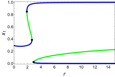
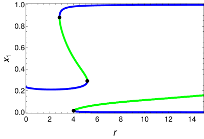
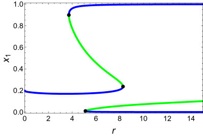
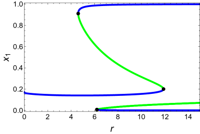
Figure 11: Bifurcation diagrams of the complete system (Equation (3)) in the asymmetric case for number of options $N=4$ in panel 11, $N=5$ in panel 11, $N=6$ in panel 11, and $N=7$ in panel 11. In all plots, the superior option’s quality is $v_{1}=8$ while the inferior options’ quality is $v_{i}=7.2,\;i\in[2,N]$, that is, $\kappa=v_{i}/v=0.9$. Blue curves represent stable equilibria and green lines unstable saddle points. Notice the increase of the range of values of $r$ in which the undecided state persists. Note also that the stable state at decision for the superior option appears earlier than the ones for the inferior alternatives. This supports a strategy to deal with the uncertainty in the decision-making scenario based on the gradual increase of $r$, which would initially bring the system into an indecision state and subsequently jump to the selection of the highest quality option.

Best of N. Figure 9 shows the stability diagrams for $N\in[4,7]$ with an underlaying density map showing the population size for the best option. While area A corresponds to the most favourable system phase, that is, there is one single attractor with a bias for the superior option, however, in the dark shaded area the population size is relatively low and might be not enough to reach a decision quorum. The dark area increases with the number of options $N$ and decreases with the difference in option’s qualities (i.e., higher $\kappa$). Therefore, for similar options, higher values of $r$ (i.e., interactions) are necessary to let the swarm make a decision.

Additionally, we report the bifurcation diagram for $N\in[4,7]$ for both the symmetric case (Figure 10) and for the asymmetric case (Figure 11).

References

- Bose et al. (2017) T. Bose, A. Reina, and J. A. R. Marshall, Curr. Opin. Behav. Sci. 6, 30 (2017).
- Conradt and Roper (2005) L. Conradt and T. J. Roper, Trends in Ecology & Evolution, Trends Ecol. Evol. 20, 449 (2005).
- Couzin et al. (2011) I. D. Couzin, C. C. Ioannou, G. Demirel, T. Gross, C. J. Torney, A. Hartnett, L. Conradt, S. A. Levin, and N. E. Leonard, Science 334, 1578 (2011).
- Marshall (2011) J. A. R. Marshall, AAAI Spring Symposium Series , 12 (2011).
- Seeley et al. (2012) T. D. Seeley, P. K. Visscher, T. Schlegel, P. M. Hogan, N. R. Franks, and J. A. R. Marshall, Science 335, 108 (2012).
- Pais et al. (2013) D. Pais, P. M. Hogan, T. Schlegel, N. R. Franks, N. E. Leonard, and J. A. R. Marshall, PLoS ONE 8, e73216 (2013).
- Ross-Gillespie and Kümmerli (2014) A. Ross-Gillespie and R. Kümmerli, Front. Microbiol. 5 (2014), 10.3389/fmicb.2014.00054.
- Kurvers et al. (2015) R. Kurvers, J. Krause, G. Argenziano, I. Zalaudek, and M. Wolf, JAMA Dermatol. 151, 1346 (2015).
- Wolf et al. (2015) M. Wolf, J. Krause, P. A. Carney, A. Bogart, and R. H. J. M. Kurvers, PLoS ONE 10, e0134269 (2015).
- Franks et al. (2003) N. R. Franks, A. Dornhaus, J. P. Fitzsimmons, and M. Stevens, Proc. R. Soc. B 270, 2457 (2003).
- Marshall et al. (2006) J. A. Marshall, A. Dornhaus, N. R. Franks, and T. Kovacs, Journal of The Royal Society Interface 3, 243 (2006).
- Marshall et al. (2009) J. A. R. Marshall, R. Bogacz, A. Dornhaus, R. Planqué, T. Kovacs, and N. R. Franks, Journal of The Royal Society Interface 6, 1065 (2009).
- Pratt and Sumpter (2006) S. C. Pratt and D. J. T. Sumpter, Proc. Natl. Acad. Sci. 103, 15906 (2006).
- Golman et al. (2015) R. Golman, D. Hagmann, and J. H. Miller, Sci. Adv. 1 (2015), 10.1126/sciadv.1500253.
- Pirrone et al. (2014) A. Pirrone, T. Stafford, and J. A. R. Marshall, Front. Neurosc. 8 (2014), 10.3389/fnins.2014.00073.
- Li et al. (2008) W. Li, H.-T. Zhang, M. Z. Chen, and T. Zhou, Phys. Rev. E 77, 021920 (2008).
- Valentini and Hamann (2015) G. Valentini and H. Hamann, Swarm Intelligence 8, 153 (2015).
- Halloy et al. (2007) J. Halloy, G. Sempo, G. Caprari, C. Rivault, M. Asadpour, F. Tâche, I. Saïd, V. Durier, S. Canonge, J. M. Amé, C. Detrain, N. Correll, A. Martinoli, F. Mondada, R. Siegwart, and J.-L. Deneubourg, Science 318, 1155 (2007).
- Hamann et al. (2012) H. Hamann, T. Schmickl, H. Wörn, and K. Crailsheim, Neural Computing and Applications 21, 207 (2012).
- McCreery et al. (2016) H. F. McCreery, N. Correll, M. D. Breed, and S. Flaxman, PLOS ONE 11, 1 (2016).
- Lindauer (1955) M. Lindauer, Zeitschrift für vergleichende Physiologie 37, 263 (1955).
- Seeley (2010) T. D. Seeley, Honeybee Democracy (Princeton University Press, 2010).
- Seeley and Buhrman (2001) T. D. Seeley and S. C. Buhrman, Behav. Ecol. Sociobiol. 49, 416 (2001).
- Franks et al. (2006) N. R. Franks, A. Dornhaus, C. S. Best, and E. L. Jones, Animal Behaviour 72, 611 (2006).
- Robinson et al. (2011) E. J. H. Robinson, N. R. Franks, S. Ellis, S. Okuda, and J. A. R. Marshall, PLoS ONE 6, e19981 (2011).
- von Frisch (1967) K. von Frisch, The Dance Language and Orientation of Bees (Harvard University Press, 1967).
- Seeley and Buhrman (1999) T. D. Seeley and S. C. Buhrman, Behav. Ecol. Sociobiol. 45, 19 (1999).
- Pratt et al. (2002) S. C. Pratt, E. B. Mallon, D. J. Sumpter, and N. R. Franks, Behav. Ecol. Sociobiol. 52, 117 (2002).
- Sumpter and Pratt (2008) D. J. T. Sumpter and S. C. Pratt, Phil. Trans. R. Soc. B 364, 743 (2008).
- Seeley and Visscher (2004) T. D. Seeley and P. K. Visscher, Behav. Ecol. Sociobiol. 56, 594 (2004).
- Reina et al. (2015a) A. Reina, G. Valentini, C. Fernádez-Oto, M. Dorigo, and V. Trianni, PLoS ONE 10, e0140950 (2015a).
- Reina et al. (2015b) A. Reina, R. Miletitch, M. Dorigo, and V. Trianni, Swarm Intelligence 9, 75 (2015b).
- Schall and Hanes (1993) J. D. Schall and D. P. Hanes, Nature 366, 467 (1993).
- (34) See Supplemental Material at [URL will be inserted by publisher] for a video of the bifurcation diagram and the phase portrait of the honeybees nest-site selection model with three options. The superior option’s quality is fixed and the value of the inferior options’ quality is systematically varied.
- Galla (2010) T. Galla, Journal of Theoretical Biology 262, 186 (2010).
- List et al. (2009) C. List, C. Elsholtz, and T. D. Seeley, Philosophical transactions of the Royal Society of London. Series B, Biological sciences 364, 755 (2009).
- Nicolis and Deneubourg (1999) S. C. Nicolis and J.-L. Deneubourg, Journal of theoretical biology 198, 575 (1999).
- Seeley (2003) T. D. Seeley, Behavioral Ecology and Sociobiology 53, 417 (2003).
- Seeley et al. (2006) T. D. Seeley, P. K. Visscher, and K. M. Passino, American Scientist 94, 220 (2006).
- Nené et al. (2012) N. R. Nené, J. Garca-Ojalvo, and A. Zaikin, PLoS ONE 7, e32779 (2012).
- Ferrell (2009) J. E. Ferrell, Molecular Cell 36, 724 (2009).
- Goentoro et al. (2009) L. Goentoro, O. Shoval, M. W. Kirschner, and U. Alon, Molec. Cell 36, 894 (2009).
- Akre and Johnsen (2014) K. L. Akre and S. Johnsen, Tr. Ecol. Evol. 29, 291 (2014).
- Couzin (2007) I. D. Couzin, Nature 445, 715 (2007).
- Marshall and Franks (2009) J. A. Marshall and N. R. Franks, Current Biology, Current Biology 19, R395 (2009).
- Couzin (2009) I. D. Couzin, Trends in Cognitive Sciences, Trends in Cognitive Sciences 13, 36 (2009).
- Passino et al. (2007) K. M. Passino, T. D. Seeley, and P. K. Visscher, Behav. Ecol. Sociobiol. 62, 401 (2007).
- Douglas et al. (1995) R. J. Douglas, C. Koch, M. Mahowald, K. a. Martin, and H. H. Suarez, Science 269, 1 (1995).
- Rutishauser et al. (2011) U. Rutishauser, R. J. Douglas, and J.-J. Slotine, Neural Computation 23, 735 (2011).
- Leonard (2014) N. E. Leonard, Annu. Rev. Contr. 38, 171 (2014).
- Reina et al. (2016) A. Reina, T. Bose, V. Trianni, and J. A. R. Marshall, in Proceedings of the 13th International Symposium on Distributed Autonomous Robotic Systems (DARS), STAR (Springer, Berlin, Germany, 2016) p. in press.
- Trianni et al. (2016) V. Trianni, A. S. Cacciapuoti, and M. Caleffi, in 2016 IEEE International Conference on Communications (ICC) (IEEE Press, 2016) pp. 1–6.