Cross-diffusion systems with non-zero flux and moving boundary conditions.
Abstract
We propose and analyze a one-dimensional multi-species cross-diffusion system with non-zero-flux boundary conditions on a moving domain, motivated by the modeling of a Physical Vapor Deposition process. Using the boundedness by entropy method introduced and developped in [5, 16], we prove the existence of a global weak solution to the obtained system. In addition, existence of a solution to an optimization problem defined on the fluxes is established under the assumption that the solution to the considered cross-diffusion system is unique. Lastly, we prove that in the case when the imposed external fluxes are constant and positive and the entropy density is defined as a classical logarithmic entropy, the concentrations of the different species converge in the long-time limit to constant profiles at a rate inversely proportional to time. These theoretical results are illustrated by numerical tests.
Introduction
The aim of this work is to propose and analyze a mathematical model for the description of a Physical Vapor Deposition (PVD) process , the different steps of which are described in details for instance in [24]. Such a technique is used in several contexts, for instance for the fabrication of thin film crystalline solar cells. The procedure works as follows: a wafer is introduced in a hot chamber where several chemical elements are injected under a gaseous form. As the latter deposit on the substrate, an heterogeneous solid layer grows upon it. Two main phenomena have to be taken into account: the first is naturally the evolution of the surface of the film; the second is the diffusion of the various species in the bulk, due to the high temperature conditions. Experimentalists are interested in controlling the external gas fluxes that are injected into the chamber, so that, at the end of the process, the spatial distributions of the concentrations of the diverse components inside the new layer are as close as possible to target profiles.
In this article, a one-dimensional model which takes into account these two factors is studied. We see this work as a preliminary step before tackling more challenging models in higher dimensions, including surfacic diffusion effects for instance. This will be the object of future work. Our main motivation for the study of such a model concerns the optimization of the external fluxes injected in the chamber during a PVD process.
More precisely, let us assume that at a time , the solid layer is composed of different chemical species and occupies a domain of the form , where denotes the thickness of the film. The evolution of is determined by the fluxes of atoms that are absorbed at the surface of the layer. At time and point , the local volumic fractions of the different species are denoted respectively by . Let us point out that if the molar volume of the solid is uniform in the thin film layer and constant during all the process, then is also equal (up to a constant multiplicative constant) to the local concentration of the species at time and point . Up to some renormalization condition, it is natural to expect that these functions are non-negative and satisfy a volumic constraint which reads as follows:
| (1) |
Because of the constraint (1), it holds that for all and . Thus, the knowledge of the functions is enough to determine the dynamics of the whole system. Replacing by , and denoting by the vector-valued function , the evolution of the concentrations inside the bulk of the solid layer is modeled through a system of cross-diffusion equations of the form
| (2) |
with approriate boundary and initial conditions, where is a matrix-valued function encoding the cross-diffusion properties of the different species.
Such systems have received much attention from the mathematical community in the case when no-flux boundary conditions are imposed on a fixed domain [19, 2, 20, 11]. Then, in arbitrary dimension , the system reads
for some fixed bounded regular domain and boundary conditions
where n denotes the outward normal unit vector to .
Such systems appear naturally in the study of population’s dynamics in biology, and in chemistry, for the study of the evolution of chemical species concentrations in a given environment [25, 12]. The analysis of these systems is a challenging task from a mathematical point of view [21, 1, 18, 27, 6, 7, 8]. Indeed, the obtained system of parabolic partial differential equations may be degenerate and the diffusion matrix is in general not symmetric and/or not positive definite. Besides, in general, no maximum principle can be proved for such systems. Nice counterexamples are given in [28]: there exist Hölder continuous solutions to certain cross-diffusion systems which are not bounded, and there exist bounded weak solutions which develop singularities in finite time.
It appears that some of these cross-diffusion systems have a formal gradient flow structure. Recently, an elegant idea, which consists in introducing an entropy density that appears to be a Lyapunov functional for these systems, has been introduced by Burger et al. in [5]. This analysis strategy, which was later extended by Jüngel in [16] and named boundedness by entropy technique, enables to obtain the existence of global in time weak solutions satisfying (1) under suitable assumptions on the diffusion matrix . It was successfully applied in several contexts (see for instance [17, 15, 29, 30]).
However, there are very few works which focus on the analysis of such cross-diffusion systems with non zero-flux boundary conditions and moving domains. To our knowledge, only systems containing at most two different species have been studied, so that and the evolution of the concentrations inside the domain are decoupled and follow independent linear heat equations [26].
The one-dimensional model (2) we propose and analyze in this paper describes the evolution of the concentration of different atomic species, with external flux boundary conditions, in the case when the diffusion matrix satisfies similar assumptions to those needed in the no-flux boundary conditions case studied in [16].
The article is organized as follows: the results of [16] in the case of no-flux boundary conditions in arbitrary dimension are recalled in Section 1. We illustrate them on a prototypical example of diffusion matrix , which is introduced in Section 1.1.
Our results in the case of a one-dimensional moving domain with non-zero flux boundary conditions are gathered in Section 2. We prove the existence of a global in time weak solution to (2) with appropriate boundary conditions and evolution law for in Section 2.2.1. The long time behaviour of a solution is analyzed in the case of constant external absorbed fluxes in 2.2.2 and an optimization problem is studied in 2.2.3. The proofs of these results are gathered in Section 3.
A numerical scheme used to approximate the solution of such systems is described in Section 4 and our theoretical results will be illustrated by several numerical tests. We refer the reader to [3] for comparisons between our proposed model and experimental results obtained in the context of thin film solar cells fabrication.
1 Case of no-flux boundary conditions in arbitrary dimension
In Section 1.1, a particular cross-diffusion model on a fixed domain with no-flux boundary conditions is presented. The latter is a prototyical example of the systems of equations considered in this paper. Its formal gradient flow structure is highlighted in Section 1.1.2. Using slight extensions of results of [29, 30], it can be seen that this system can be analyzed using the theoretical framework developped in [16, 5], which is recalled in Section 1.2.
Throughout this section, let us denote by the space dimension, the regular bounded domain occupied by the solid. The local concentrations at time and position of the different atomic species entering in the composition of the material are respectively denoted by . We also denote by n the normal unit vector pointing outwards the domain .
1.1 Example of cross-diffusion system
1.1.1 Presentation of the model
As mentioned above, we have one particular example of system of cross-diffusion equations in mind, which is used to illustrate more general theoretical results. This system, with no-flux boundary conditions, reads as follows : for any ,
| (3) |
where for all , the positive real numbers satisfy . They represent the cross-diffusion coefficients of atoms of type with atoms of type . This set of equations can be formally derived from a discrete stochastic lattice hopping model, which is detailed in the Appendix.
The initial condition of this system is assumed to satisfy:
| (4) |
The relationship is a natural volumic constraint which encodes the fact that each site of the crystalline lattice of the solid has to be occupied (vacancies being treated as a particular type of atomic species).
Summing up the equations of (3), we observe that a solution must necessarily satisfy . It is thus expected that the following relationship should hold:
| (5) |
Plugging the expression in (3), it holds that for all ,
Thus, the system can be rewritten as a function of as follows
| (6) |
where and the matrix-valued application
is defined by
| (7) |
Despite their importance in chemistry or biology, it appears that the mathematical analysis of systems of the form (6), taking into account constraints (5), is quite recent [5, 11, 16, 22]. Let us point out here that the non-negativity of the solutions to (6) through time is a mathematical issue, linked to the absence of a maximum principle for such systems.
At least up to our knowledge, the first proof of existence of global weak solutions of (6) satisfying constraints (5) with non-identical cross-diffusion coefficients is given in [5] for with coefficients such that for and . These results were later extended in [30] to a general number of species with cross-diffusion coefficients satisfying and for all ; the authors of the latter article proved in addition the uniqueness of such weak solutions. In [29], the case with arbitrary positive coefficients is covered, though no uniqueness result is provided. The main difficulty of the mathematical analysis of such equations relies in the bounds (5), which are not obvious since no maximum principle can be proved for these systems in general. In all the articles mentioned above, the analysis framework used by the authors is the so-called boundedness by entropy method. The main idea of this technique is to write the above system of equations as a formal gradient flow and derive estimates on the solutions using the decay of some well-chosen entropy functional. We present in Section 1.1.2 the formal gradient flow structure of (6) and recall the results of [16] in Section 1.2.
1.1.2 Formal gradient flow structure of (6)
We detail in this section the formal gradient flow structure of the system (6).
Let be defined by
| (9) |
Let us introduce the classical entropy density (see for instance [5], [16], [30] and [22])
| (10) |
where . Some properties of can be easily checked:
-
(P1)
the function belongs to ; consequently, is bounded on ;
-
(P2)
the function is strictly convex on ;
-
(P3)
its derivative
is invertible and its inverse is given by
In the following, we denote by the Hessian of . The entropy functional is defined by
| (11) |
Throughout the article, for all , we shall denote by the measurable vector-valued function defined by
The system (6) can then be formally rewritten under the following gradient flow structure
| (12) |
where is the so-called mobility matrix of the system defined for all by
More precisely, it holds that for all , where for all ,
| (13) |
1.2 Existence of global weak solutions by the boundedness by entropy technique
The formal gradient flow formulation of a system of cross-diffusion equations is a key point in the boundedness by entropy technique. In the example presented in Section 1.1, it implies in particular that is a Lyapunov functional for the system (6) [5, 16]. However, the mobility matrix obtained for these systems is not a concave function of the densities, so that standard gradient flow theory arguments (such as the minimizing movement method) cannot be applied in this context [31, 9, 14, 22]. However, the existence of a global weak solution to (6) can still be proved. Let us recall here a simplified version of Theorem 2 of [16] which is adapted to our context.
Theorem 1 (Theorem 2 of [16]).
Let be the domain defined by (9). Let be a matrix-valued functional defined on satisfying and the following assumptions:
-
(H1)
There exists a bounded from below convex function such that its derivative is invertible on ;
-
(H2)
There exists , and for all , there exist such that for all and ,
Let so that . Then, there exists a weak solution with initial condition to
| (14) |
such that for almost all , with
Lemma 1 states that the prototypical example presented in Section 1.1 falls into the framework of Theorem 1. The proof of the latter is given Section 3.1 for the sake of completeness, and relies on ideas introduced in [30].
Lemma 1.
The existence of global weak solutions to (6) is then a direct consequence of Theorem 1 and Lemma 1.
Let us point out that the uniqueness of solutions to general systems of the form (14) remains an open theoretical question, at least up to our knowledge. It can be obtained in some particular cases. When the diffusion matrix is defined by (7) and when all the diffusion coefficients are identically equal to some constant , the uniqueness of the solution can be trivially obtained since the system boils down to a set of decoupled heat equation for the evolution of the density of each species.
2 Case of non-zero flux boundary conditions and moving domain
In the sequel, we restrict the study to the case when . In this section, we propose a model for the description of a PVD process and present theoretical results whose proofs are postponed to Section 3. The global existence of a weak solution is proved. The long-time behaviour of such a solution is studied in the case of constant external fluxes. Lastly, under the assumption that the coefficients are chosen so that there is a unique solution to the system, we prove the existence of a solution to an optimization problem.
2.1 Presentation of the model
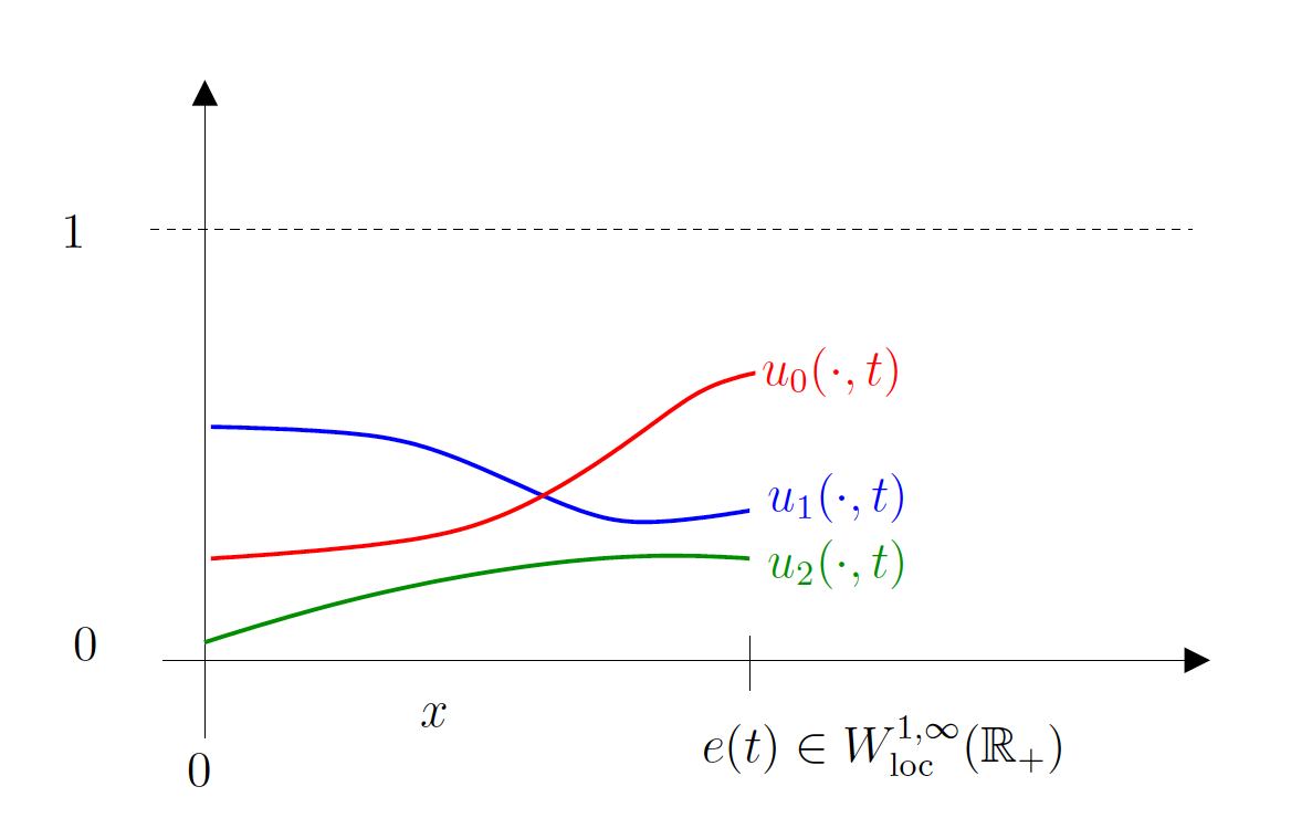
For the sake of simplicity, we assume that non-zero fluxes are only imposed on the right-hand side of the domain occupied by the solid. At some time , this domain is denoted by where models the thickness of the layer. Initially, we assume that the domain occupied by the solid at time is the interval for some initial thickness .
The evolution of the thickness of the film is determined by the external fluxes of the atomic species that are absorbed at its surface. More precisely, let us assume that there are different chemical species composing the solid layer and let belong to . For all , the function represents the flux of the species absorbed at the surface at time and is assumed to be non-negative. In this one-dimensional model, the evolution of the thickness of the solid is assumed to be given by
| (15) |
In the following, we will denote by (see Figure 1).
For all and , the local concentration of species at time and point is denoted by . The evolution of the vector is given by the system of cross-diffusion equations
| (16) |
where is a well-chosen diffusion matrix satisfying (H1)-(H2).
We consider that for every , the system satisfies the following conditions on the boundary :
| (17) |
An easy calculation shows that these boundary conditions, in addition to (15) and (16), ensure that, for all ,
Indeed, it holds that
The calculation for the species reads:
To sum up, the final system of interest reads:
| (18) |
where is an initial condition satisfying for almost all . We assume in addition that belongs to .
2.1.1 Rescaled version of the model
We introduce here a rescaled version of system (18). For all , and , let us denote by . It holds that
where . Thus, is a solution of (18) if and only if is a solution to the following system:
| (19) |
where .
Proving the existence of a global weak solution to (18) is equivalent to proving the existence of a global weak solution to (19).
Actually, it can be seen that the entropy of the system (19) satisfies a formal inequality at the continuous level which is at the heart of the proof of our existence result. Indeed, let us denote by
where is a solution to (19). Then, formal calculations yield that
Denoting by , it holds that for all . Besides, using assumption (H2), we obtain that
which yields that
Using the convexity of , we obtain that , so that
| (20) |
Inequality (20) is not an entropy dissipation inequality in the sense that the quantity may increase with time. However, using the fact and assumption (H3), it implies that the quantity cannot blow up in finite time, which is sufficient for our purpose.
2.2 Theoretical results
2.2.1 Global in time existence of weak solutions
Our first result deals with the global in time existence of bounded weak solutions to (19) (and thus to (18)).
Theorem 2.
Let . Let be a matrix-valued functional satisfying and assumptions (H1)-(H2) of Theorem 1 for some well-chosen entropy density . We assume in addition that
-
(H3)
.
Let , so that and . Let us define for almost all , and . Then, there exists a weak solution with initial condition to (19) such that for almost all , . Besides,
In particular, .
Let us point out that the example described in Section 1.1 satisfies all the assumptions of Theorem 2 since the entropy density defined by (10) belongs to . Let us also point here that the form of (19) is different from the system considered in [16] through i) the boundary conditions and ii) the existence of the drift term .
2.2.2 Long-time behaviour for constant fluxes
In the case when the fluxes are constant in time, we obtain long-time asymptotics for the functions , provided that the entropy density is given by (10). More precisely, the following result holds:
Proposition 1.
Under the assumptions of Theorem 2, let us make the following additional hypotheses:
-
(T1)
for all , there exists so that , for all ;
-
(T2)
for all , the entropy density can be chosen so that .
For all , let us define and by . Let us also denote by
the relative entropy associated to and . Then, there exists a global weak solution to (19) and a constant such that
| (21) |
and
| (22) |
The proof of Proposition 1 is given in Section 3.3. Numerical results presented in Section 4 illustrate the rate of convergence of the rescaled concentrations to constant profiles in .
Let us comment here on assumption (T2). Actually, in the proof, we use the following properties of the logarithmic entropy density:
-
•
and if satisfies , then necessarily ;
-
•
There exists a constant vector such that for all , .
-
•
The relative entropy density satisfies a Csizàr-Kullback type inequality.
Similar long-time asymptotics results can be obtained for general entropy densities satisfying these three properties. For the sake of simplicity, we chose to restrict ourselves to the case of logarithmic entropy density in Proposition 1.
The central ingredient of the proof is the following formal entropy inequality. In the case when is given by (10), it can be easily seen that is also a valid entropy density for the diffusion coefficient in the sense that also satisfies assumptions (H1)-(H2)-(H3). Thus, inequality (20) holds with instead of so that
where for all , . Denoting by , it holds that and for all . Finally, using the fact that and that , we obtain that
This inequality implies that there exists a constant such that for all ,
The rates on the norm of the solutions are then obtained using the Csizàr-Kullback inequality.
2.2.3 Optimization of the fluxes
As mentioned in the introduction, our main motivation for studying this system is the control of the gazeous fluxes injected during a PVD process. It is assumed here that the wafer remains in the hot chamber where the different atomic species are injected during a time . The cross-diffusion phenomena occur in the bulk of the thin film layer because of the high temperatures that are imposed during the process. Once the wafer is taken out of the chamber, the composition of the film is freezed and no diffusion phenomena take place anymore. The profiles of the local volumic fractions of the different chemical species in the film thus remain unchanged after the time . It is of practical interest to adapt the fluxes through time so that these final concentration profiles are as close as possible to target functions chosen a priori.
Let be the initial thickness of the solid. In practice, the maximal value of the fluxes which can be injected is limited due to device constraints. Let and let us then denote by . For all , we denote by the time-dependent thickness of the film, and by a solution to (19) associated with the external fluxes .
Let us point out here the uniqueness of a solution to (18) (or (19)) remains an open problem in general. When the diffusion matrix is defined by (7), the only case for which uniqueness of a global solution can be obtained is the trivial case where the cross-diffusion coefficients are identical to some constant for all . Indeed, in this case, it can be seen that the system (19) can be written as a set of independent advection-diffusion PDEs on each of the rescaled concentration profiles (). Thus, we will have to make some assumption on the cross-diffusion coefficients in the general case.
We make the following assumption on the diffusion matrix :
-
(C1)
For any , there exists a unique global weak solution to system (19) so that for almost all , .
The goal of the optimization problem consists in the identification of optimal time-dependent non-negative functions so that the final thickness of the film and the (rescaled) concentration profiles for the different chemical species at the end of the fabrication process are as close as possible to desired targets denoted by and .
The real-valued functional defined by
| (23) |
is the cost function we consider here. More precisely, we have the following result, which is proved in Section 3.4.
Proposition 2.
Under the assumptions of Theorem 2, let us make the additional assumption (C1). Then, the functional is well-defined and there exists a minimizer to the minimization problem
| (24) |
Of course, uniqueness of such a solution is not expected in general.
3 Proofs
3.1 Proof of Lemma 1
Let us prove that the matrix-valued function defined in (7) satisfies the assumptions of Theorem 1 with the entropy functional given by (10).
As mentioned in Section 1.1, the entropy density belongs to (thus is bounded on ), is strictly convex on , and its derivative is invertible. As a consequence, satisfies assumption (H1) of Theorem 1.
Let us now prove that assumption (H2) of Theorem 1 is satisfied with for all . To this aim, we follow the same strategy of proof as the one used in [30]. Let us prove that there exists such that for all ,
| (25) |
This inequality implies (H2) with and for all .
Let . We have for all ,
Introducing , where for all ,
it holds that . Thus, . It can be easily checked that , where has the same structure as but with diffusion coefficients instead of , and where for all .
On the one hand, where is the matrix whose all coefficients are identically equal to . Since the matrix is a semi-definite positive matrix, so is .
On the other hand, since is strictly convex on , is semi-definite positive if and only if is semi-definite positive. Indeed, for all , we have . It can be observed that , where for all ,
For all , we have
The matrix is indeed a semi-definite positive matrix. Hence we have proved inequality (25), which yields the desired result.
3.2 Proof of Theorem 2
For the sake of simplicity, we will prove the existence of a solution on the finite time interval where is an arbitrary positive constant. Actually, the proof can be easily adapted to obtain the existence of a global solution for an infinite time horizon.
The proof follows similar lines as the proof of Theorem 2 of [16] and is divided in three main steps. Firstly, an approximate time-discrete problem is introduced for which uniform bounds are proved in a second step. Lastly, passing to the limit in this approximate problem using the obtained bounds enables to obtain the existence of a weak solution.
3.2.1 Step 1 : Approximate time-discrete problem
Let us first assume at this point that belong to .
Let , and . For all so that , let us denote by , and . Let us also define
| (26) |
so that and .
By assumption, belongs to . In the rest of the proof, for any , we denote by and by .
Let us already mention at this point that the (formal) weak formulation of (19) reads as follows: for all ,
Let us first prove the following lemma.
Lemma 2.
Assume that . Then, for all such that , there exists solution of
| (27) | ||||
for all . Besides, the following discrete inequality holds for all such that ,
| (28) | ||||
3.2.2 Step 2: Uniform bounds
For all , let be a sequence of non-negative functions of which weakly-* converges to in as goes to infinity, and for all ,
Let us define
It holds that strongly converges to in . Indeed, let . Since is continuous on , it is uniformly continuous, and there exists so that for all satisfying , then . Let and so that for all , . Then, it holds that
because of the weak-* convergence in of to for all .
Thus, there exists large enough such that for all , . Besides, the non-negativity of the functions and implies that and are non-decreasing functions, so that for all and all ,
As a consequence, for all , all and all ,
Hence, for all , , which yields the strong convergence of the sequence to in .
For all such that , we denote by a solution to (27) associated to the fluxes . The time-discretized associated quantities are denoted (using obvious notation) by , and .
Let us define the piecewise constant in time functions , , , and as follows: for all such that , and almost all ,
Besides, let us set and . Let us also denote by the components of .
Then, the following system holds for all piecewise constant in time functions ,
| (31) | ||||
The set of piecewise constant functions in time is dense in , so that (31) also holds for any .
Using the fact that satisfies assumption (H2) of Theorem 1 and the fact that , we obtain for all such that ,
where for all and for all . It follows from (30) that for all such that ,
Summing these inequalities yields, for so that ,
| (32) | ||||
In the sequel, will denote an arbitrary constant, which may change along the calculations, but remains independent on , , and . We are deliberately keeping here the explicit dependence of the constants on in view of the proof of Proposition 2. It then holds that
We also obtain from (32) and the fact that for all that
| (33) |
and
| (34) |
Since for all , , this implies that
| (35) | ||||
Besides,
| (36) | ||||
using the fact that .
This yields that for all ,
This last inequality shows that
| (37) |
3.2.3 Step 3: The limit and
For all , the functions and are continuous on , and hence are uniformly continuous. As a consequence, there exists small enough so that for any satisfying , then and . This implies in particular that
These inequalities, together with the fact that weakly-* converges to in (respectively that strongly converges to in ), imply that the sequence (respectively ) also weakly-* converges to in (respectively strongly converges to in ).
In the following, we consider such a subsequence . The uniform estimates (37) and (35) allow us to apply the Aubin lemma in the version of Theorem 1 of [10]. Up to extracting a subsequence which is not relabeled, there exists so that as goes to infinity and goes to ,
Because of the boundedness of in , the convergence even holds strongly in for any , which is a consequence of the dominated convergence theorem. The latter theorem, together with implies also that the convergence holds strongly in . Moreover, using (36) and (34), up to extracting another subsequence, there exists so that
The strong convergence of in and the weak convergence of in implies necessarily that .
We are now in position to pass to the limit and in (31) with and . Let us recall that (respectively ) converges strongly (respectively weakly-*) to (respectively ) in . We obtain that is a solution to
| (38) | ||||
yielding the result.
3.2.4 Proof of Lemma 2
Proof of Lemma 2.
We prove Lemma 2 by induction using the Leray-Schauder fixed-point theorem. Let and . We consider the following linear problem: find solution of
| (39) |
where
and
As a consequence of (H2), the matrix is positive semi-definite for any . Thus, the bilinear form is coercive and continuous on , and it holds that
| (40) |
Since and , the linear form is continuous. From the Agmon inequality, there exists independent of , or such that for all ,
| (41) |
where . It immediately follows from the Lax-Milgram theorem that there exists a unique solution to (39).
We define the operator as follows. For all and , is the unique solution of (39). We are going to prove that there exists a fixed-point of the equation using the Leray-Schauder fixed-point theorem (Theorem 3 in the Appendix). This will end the proof of Lemma 2 since such a fixed-point is a solution of (27).
Let us check that all the assumptions of Theorem 3 are satisfied:
-
(A1)
For all , ;
-
(A2)
Let us prove that is a compact map. To this aim, let us first prove that it is continuous. Let and be sequences in and respectively, and so that and strongly in . For all , let . From assumption (H1) and the global inversion theorem, is a -diffeomorphism. Thus, together with the fact that , it holds that the applications and are continuous. Hence, and strongly in and respectively.
Besides, the uniform coercivity and continuity estimates (40) and (41) imply that is a bounded sequence in . Thus, up to the extraction of a subsequence which is not relabeled, weakly converges to some in . Passing to the limit in (39) implies that . The uniqueness of the limit yields that the whole sequence weakly converges to in . The convergence thus holds strongly in because of the compact embedding . This proves the continuity of the map and its compactness follows again from the compact embedding .
-
(A3)
Let and so that . It holds that (taking as a test function in (39) with ),
(42) (43) Let us consider separately the different terms appearing in (43). First, by convexity of , and using the fact that , it holds that
(44) Besides, using an integration by parts,
(45) Using (26), we obtain
(46) Finally, using (43), (44), (45) and (46), and again the convexity of , we obtain
(47) This inequality implies that
for some constant independent of , of .
3.3 Proof of Proposition 1
Let us define by , and . From (T1), the vector obviously belongs to the set .
If defined by (10) is an entropy density for which satisfies assumptions (H1)-(H2)-(H3), then satisfies the same assumptions with the entropy density
Indeed, for all , , where is a constant vector in and . Moreover, the entropy density has the following interesting property: is the unique minimizer of on so that for all . In the rest of the proof, for all , we will denote by .
Let be a sequence of solutions to the regularized time-discrete problems (27) defined in Lemma 2 with the constant fluxes and the entropy density . The entropy inequality (28) then reads
| (48) | ||||
In our particular case, for all , , and , so that we obtain
This implies that for all and ,
| (49) |
Let us denote by the piecewise constant in time function defined by
Let and such that a.e. in . Inequality (49) and Fubini’s theorem for integrable functions implies that
From the proof of Theorem 2, we know that up to the extraction of a subsequence which is not relabeled, converges strongly in and a.e. in as and go to zero to a global weak solution to (19). Using Lebesgue dominated convergence theorem, and passing to the limit in the above inequality yields
which implies that there exists such that for almost all ,
| (50) |
which yields inequality (21). In the rest of the proof, will denote an arbitrary positive constant independent on the time . Furthermore, since , it holds that from [23], and the Lebesgue dominated convergence theorem implies that is a continuous function. Inequality (50) then holds for all .
For all , let us denote by . By convention, we define and . It can be checked from the weak formulation of (27) that
Passing to the limit using the Lebesgue dominated convergence theorem, we obtain that for almost all ,
so that . The continuity of implies that this equality holds for all .
3.4 Proof of Proposition 2
Let be a minimizing sequence for i.e such that
By definition of the set , the sequence is bounded in . Thus, up to a non relabeled extraction, it weakly-* converges to some limit in . As a consequence, (respectively ) converges weakly-* (respectively strongly) in to (respectively ).
For each , let be the unique global weak solution to (19) associated to the fluxes . Its uniqueness is a consequence of assumption (C1). From the bounds obtained in the proof of Theorem 2 and the boundedness of in , it holds that the sequences , and are also uniformly bounded in .
Thus, up to the extraction of a subsequence which is not relabeled, using the compact injection of into (see [23]), there exists and so that
Using similar arguments as in the proof of Theorem 2, we also obtain that is necessarily equal to . Passing to the limit , we obtain that for all ,
Assumption (C1) yields . The above convergence results then imply that
and hence is a minimizer of problem (24). Hence the result.
4 Numerical tests
In this section, we present some numerical tests illustrating the results of Section 2 on the prototypical example of Section 1.1. In Section 4.1, we present the numerical scheme used in our simulations to compute an approximation of a solution of (19). In Section 4.2 and Section 4.3, some numerical tests which illustrate Proposition 1 and Proposition 2 are detailed.
4.1 Discretization scheme
In view of the optimization problem (24) we are aiming at, it appears that a fully implicit unconditionally stable scheme is needed to allow the use of reasonably large time steps.
We present here the numerical scheme used for the discretization of (19), for the particular model presented in Section 1.1. We do not provide a rigorous numerical analysis for this scheme here.
Let and . We define for all , . The discrete external fluxes are characterized for every by vectors , where . For every , the thickness of the thin film and it derivative at time are approximated respectively by
In addition, let and and . For all , and , we denote by the finite difference approximation of at time and point . Here again, we use the convention that .
We use a centered second-order finite difference scheme for the diffusive part of the equation, and a first-order upwind scheme for the advection part, together with a fully implicit time scheme. Assuming that the approximation is known, one computes as solutions of the following sets of equations.
For all and ,
| (51) | ||||
together with boundary conditions which reads for all ,
| (52) | ||||
| (53) |
The nonlinear system of equations (51)-(52)-(53), whose unknowns are is solved using Newton iterations with initial guess . The obtained solution does not satisfy in general the desired non-negativeness and volumic constraints. This is the reason why an additional projection step is performed. For all and , we define
so that
We numerically observe that this scheme is unconditionally stable with respect to the choice of discretization parameters and .
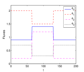
A standard practice in the production of thin film CIGS (Copper, Indium, Gallium, Selenium) solar cells by means of PVD process is to consider piecewise-constant external fluxes. We refer the reader to [3] for further details. In the following numerical tests, we consider time-dependent functions of the form
| (54) |
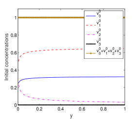
where and are non-negative constants for all . Besides, we consider initial condition of the form
| (55) |
where are functions which will be precised below. In the whole section, system (19) is simulated with four species (i.e. ).
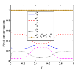
In Figure 2 are plotted the results obtained for the simulation of (19) with the following parameters :
The profile of the external fluxes is plotted in Figure 2-(a). In Figure 2-(b) and Figure 2-(c) are given respectively the the initial and the final concentrations of the four species.
4.2 Long-time behaviour results
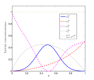
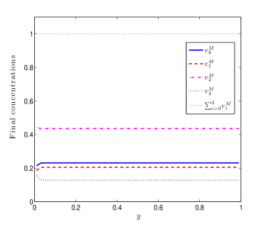
In this section is given a numerical illustration of Proposition 1. We consider time-dependent functions of the form
| (56) |
where . In Figure 3 are plotted the results obtained for the the simulation of (19) with the following parameters :
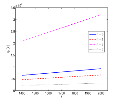
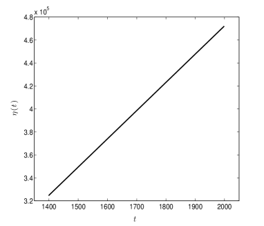
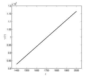
For all , let . We consider the time-dependent quantity
where the relative entropy is defined in (21). We also consider the quantities
and
In Figure 3-(a) and 3-(b) are plotted respectively the initial and the final concentration profiles.
The evolution of (respectively and ) with respect to is shown in Figure 3-(c) (respectively 3-(d) and 3-(e)). We numerically observe that these quantities are affine functions of in the asymptotic regime which illustrates the theoretical result of Proposition 1.
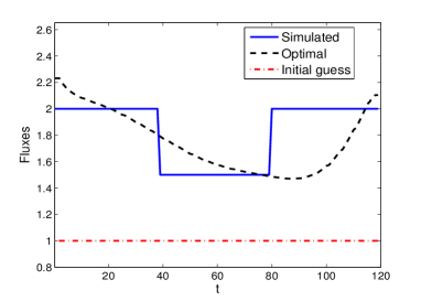
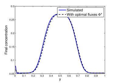
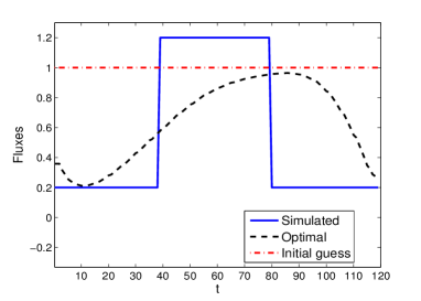
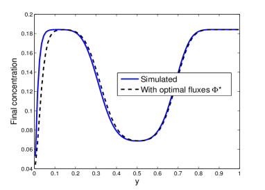
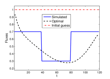
4.3 Optimization of the fluxes
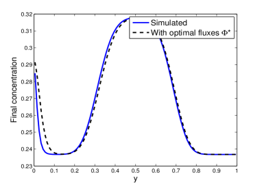
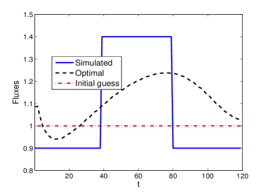
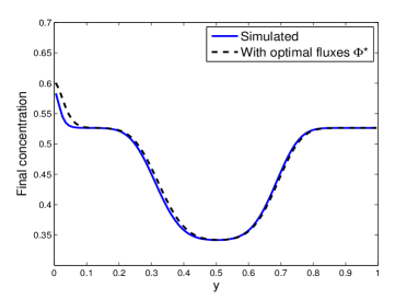
The optimization problem (24) is solved in practice using an adjoint formulation associated to the discretization scheme described in Section 4.1. We refer the reader to [3] for more details and comparisons between our model and experimental results obtained in the context of thin film CIGS solar cell fabrication. To illustrate Proposition 2, we proceed as follows: first, we perform a simulation of (19) with external fluxes for a duration to obtain a final thickness and final concentrations , then, we solve the minimization problem (24) to obtain optimal fluxes where the target concentrations are
and the target thickness is
Lastly, we perform another simulation of (19) with the obtained optimal fluxes and compare the final concentrations and the final thickness to the target concentrations and the target thickness .
In Figures 4-(a), 5-(a), 6-(a) and 7-(a) are plotted the final concentration profiles resulting from the simulation of (19) with the following parameters :
-
•
, , , , , .
-
•
Cross-diffusion coefficients
-
•
External fluxes of the form (54) with
-
•
Initial concentrations of the form (55) with , , and .
We use a quasi-Newton iterative gradient algorithm for the resolution of the minimization problem. At each iteration of the algorithm, the approximate hessian is updated by means of a BFGS procedure and the optimal step size is the solution of a line search subproblem. More details on the numerical optimization algorithms can be found in [13]. The initial guess is taken of the form (56) where for all .
The algorithm is run until one of the following stopping criterion is reached : either or with and .
In Figure 8-(a) we plot the evolution of the value of the cost with respect to the number of iterations. We refer the reader to [3] for more details and comparison between different minimization approaches.
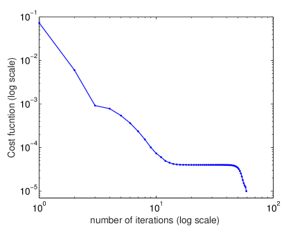
We numerically observe that all the concentrations are well reconstructed and that the value of the optimal thickness is close to the target thickness . Unlike the external fluxes , the optimal fluxes are not piecewise constant. These tests show that the uniqueness of a solution to the optimization problem (24) can not be expected in general. We refer the reader to [3] for results obtained in the case of the control of PVD process for the fabrication of this film solar cells.
5 Conclusion
In this work, we propose and analyze a one-dimensional model for the description of a PVD process. The evolution of the local concentrations of the different chemical species in the bulk of the growing layer is described via a system of cross-diffusion equations similar to the ones studied in [5, 16]. The growth of the thickness of the layer is related to the external fluxes of atoms that are absorbed at the surface of the film.
The existence of a global weak solution to the final system using the boundedness by entropy method under assumptions on the diffusion matrix of the system close to those needed in [16] is established. In addition, the entropy density is required to be continuous (hence bounded) on the set .
We prove the existence of a solution to an optimization problem under the assumption that there exists a unique global weak solution to the obtained system, whatever the value of the external fluxes.
Lastly, in the case when the entropy density is defined by , we prove in addition that, when the external fluxes are constant and positive, the local concentrations converge in the long time to a constant profile at a rate which scales like .
A discretization scheme, which is observed to be unconditionnaly stable, is introduced for the discretization of (19). This scheme enables to preserve constraints (5) at the discretized level.
We see this work as a preliminary step before tackling related problems in higher dimension, including surfacic diffusion effects. Besides, the proof of assumption (C1) remains an open question in general at least to our knowledge. Lastly, a nice theoretical question which is not tackled in this paper, but will be the object of future research, is the characterization of the set of reachable concentration profiles.
6 Acknowledgements
We are very grateful to Eric Cancès and Tony Lelièvre for very helpful advice and discussions. We would like to thank Jean-François Guillemoles, Marie Jubeault, Torben Klinkert and Sana Laribi from IRDEP, who introduced us to the problem of modeling PVD processes for the fabrication of thin film solar cells. The EDF company is acknowledged for funding. We would also like to thank Daniel Matthes for very helpful discussions on the theoretical part and the reviewers whose comments helped in very significantly improving the quality of the paper.
7 Appendix
7.1 Formal derivation of the diffusion model (3)
We present in this section a simplified formal derivation of the cross-diffusion model (3) from a one-dimensional microscopic lattice hopping model with size exclusion, in the same spirit than the one proposed in [5].
We consider here a solid occupying the whole space and discretize the domain using a uniform grid of step size . At any time , we denote by the number of atoms of type () in the interval (). Let denote a small enough time step. We assume that during the time interval , an atom located in the interval can exchange its position with an atom of type () located in one of the two neighbouring intervals with probability . In average, we obtain the following evolution equation for :
This yields that
Choosing and so that these quantities satisfy a classical diffusion scaling , denoting by and letting the time step and grid size go to , we formally obtain the following equation for the evolution of on the continuous level:
which is identical to the system of equations (3) introduced in the first section. Of course, this formal argument can be easily extended to any arbitrary dimension.
7.2 Leray-Schauder fixed-point theorem
Theorem 3 (Leray-Schauder fixed-point theorem).
Let be a Banach space and be a continuous map such that
-
(A1)
for each ;
-
(A2)
is a compact map;
-
(A3)
there exists a constant such that for each pair which satisfies , we have .
Then, there exists a fixed-point satisfying .
References
- [1] Nicholas D Alikakos. Lp bounds of solutions of reaction-diffusion equations. Communications in Partial Differential Equations, 4(8):827–868, 1979.
- [2] Herbert Amann et al. Dynamic theory of quasilinear parabolic equations. ii. reaction-diffusion systems. Differential and Integral Equations, 3(1):13–75, 1990.
- [3] Athmane Bakhta. Mathematical models and numerical simulation of photovoltaic devices. PhD thesis, in preparation, 2017.
- [4] Laurent Boudin, Bérénice Grec, and Francesco Salvarani. A mathematical and numerical analysis of the maxwell-stefan diffusion equations. Discrete and Continuous Dynamical Systems-Series B, 17(5):1427–1440, 2012.
- [5] Martin Burger, Marco Di Francesco, Jan-Frederik Pietschmann, and Bärbel Schlake. Nonlinear cross-diffusion with size exclusion. SIAM Journal on Mathematical Analysis, 42(6):2842–2871, 2010.
- [6] Li Chen and Ansgar Jüngel. Analysis of a multidimensional parabolic population model with strong cross-diffusion. SIAM journal on mathematical analysis, 36(1):301–322, 2004.
- [7] Li Chen and Ansgar Jüngel. Analysis of a parabolic cross-diffusion population model without self-diffusion. Journal of Differential Equations, 224(1):39–59, 2006.
- [8] Marco Di Francesco and Jesús Rosado. Fully parabolic keller–segel model for chemotaxis with prevention of overcrowding. Nonlinearity, 21(11):2715, 2008.
- [9] Jean Dolbeault, Bruno Nazaret, and Giuseppe Savaré. A new class of transport distances between measures. Calculus of Variations and Partial Differential Equations, 34(2):193–231, 2009.
- [10] Michael Dreher and Ansgar Jüngel. Compact families of piecewise constant functions in lp (0, t; b). Nonlinear Analysis: Theory, Methods & Applications, 75(6):3072–3077, 2012.
- [11] Jens André Griepentrog and Lutz Recke. Local existence, uniqueness and smooth dependence for nonsmooth quasilinear parabolic problems. Journal of Evolution Equations, 10(2):341–375, 2010.
- [12] Thomas Hillen and Kevin J Painter. A user’s guide to pde models for chemotaxis. Journal of mathematical biology, 58(1-2):183–217, 2009.
- [13] Claude Lemaréchal J.Frédéric Bonnans, Jean Charles Gilbert and Claudia Sagastizàbal. Numerical Optimization. Theoretical and Practical Aspects, volume 1. Springer-Verlag Berlin Heidelberg, 2006.
- [14] Richard Jordan, David Kinderlehrer, and Felix Otto. The variational formulation of the fokker–planck equation. SIAM journal on mathematical analysis, 29(1):1–17, 1998.
- [15] Ansgar Juengel and Ines Viktoria Stelzer. Entropy structure of a cross-diffusion tumor-growth model. Mathematical Models and Methods in Applied Sciences, 22(07):1250009, 2012.
- [16] Ansgar Jüngel. The boundedness-by-entropy method for cross-diffusion systems. Nonlinearity, 28(6):1963, 2015.
- [17] Ansgar Jungel and Ines Viktoria Stelzer. Existence analysis of maxwell–stefan systems for multicomponent mixtures. SIAM Journal on Mathematical Analysis, 45(4):2421–2440, 2013.
- [18] Konrad Horst Wilhelm Küfner. Invariant regions for quasilinear reaction-diffusion systems and applications to a two population model. Nonlinear Differential Equations and Applications NoDEA, 3(4):421–444, 1996.
- [19] Olga A Ladyzenskaja and Vsevolod A Solonnikov. Nn ural ceva, linear and quasilinear equations of parabolic type, translated from the russian by s. smith. translations of mathematical monographs, vol. 23. American Mathematical Society, Providence, RI, 63:64, 1967.
- [20] Dung Le and Toan Trong Nguyen. Everywhere regularity of solutions to a class of strongly coupled degenerate parabolic systems. Communications in Partial Differential Equations, 31(2):307–324, 2006.
- [21] Thomas Lepoutre, Michel Pierre, and Guillaume Rolland. Global well-posedness of a conservative relaxed cross diffusion system. SIAM Journal on Mathematical Analysis, 44(3):1674–1693, 2012.
- [22] Matthias Liero and Alexander Mielke. Gradient structures and geodesic convexity for reaction–diffusion systems. Phil. Trans. R. Soc. A, 371(2005):20120346, 2013.
- [23] Jacques Louis Lions and Enrico Magenes. Non-homogeneous boundary value problems and applications, volume 1. Springer Science & Business Media, 2012.
- [24] Donald M Mattox. Handbook of physical vapor deposition (PVD) processing. William Andrew, 2010.
- [25] Kevin J Painter. Continuous models for cell migration in tissues and applications to cell sorting via differential chemotaxis. Bulletin of Mathematical Biology, 71(5):1117–1147, 2009.
- [26] Jacobus W Portegies and Mark A Peletier. Well-posedness of a parabolic moving-boundary problem in the setting of wasserstein gradient flows. arXiv preprint arXiv:0812.1269, 2008.
- [27] Reinhard Redlinger. Invariant sets for strongly coupled reaction-diffusion systems under general boundary conditions. Archive for Rational Mechanics and Analysis, 108(4):281–291, 1989.
- [28] Jana Stará and Oldrich John. Some (new) counterexamples of parabolic systems. Commentationes Mathematicae Universitatis Carolinae, 36(3):503–510, 1995.
- [29] Nicola Zamponi and Ansgar Jüngel. Analysis of degenerate cross-diffusion population models with volume filling. In Annales de l’Institut Henri Poincare (C) Non Linear Analysis. Elsevier, 2015.
- [30] Nicola Zamponi and Ansgar Jüngel. Analysis of degenerate cross-diffusion population models with volume filling. In Annales de l’Institut Henri Poincare (C) Non Linear Analysis. Elsevier, 2015.
- [31] Jonathan Zinsl and Daniel Matthes. Transport distances and geodesic convexity for systems of degenerate diffusion equations. Calculus of Variations and Partial Differential Equations, 54(4):3397–3438, 2015.