Knapsack Problems: A Parameterized Point of View

Abstract

The knapsack problem (KP) is a very famous NP-hard problem in combinatorial optimization. Also its generalization to multiple dimensions named d-dimensional knapsack problem (d-KP) and to multiple knapsacks named multiple knapsack problem (MKP) are well known problems. Since KP, d-KP, and MKP are integer-valued problems defined on inputs of various informations, we study the fixed-parameter tractability of these problems. The idea behind fixed-parameter tractability is to split the complexity into two parts - one part that depends purely on the size of the input, and one part that depends on some parameter of the problem that tends to be small in practice. Further we consider the closely related question, whether the sizes and the values can be reduced, such that their bit-length is bounded polynomially or even constantly in a given parameter, i.e. the existence of kernelizations is studied. We discuss the following parameters: the number of items, the threshold value for the profit, the sizes, the profits, the number $d$ of dimensions, and the number $m$ of knapsacks. We also consider the connection of parameterized knapsack problems to linear programming, approximation, and pseudo-polynomial algorithms.

Keywords: knapsack problem; d-dimensional knapsack problem; multiple knapsack problem; parameterized complexity; kernelization

1 Introduction

The knapsack problem is one of the famous tasks in combinatorial optimization. In the knapsack problem (KP) we are given a set $A$ of $n$ items. Every item $j$ has a profit $p_{j}$ and a size $s_{j}$. Further there is a capacity $c$ of the knapsack. The task is to choose a subset $A^{\prime}$ of $A$, such that the total profit of $A^{\prime}$ is maximized and the total size of $A^{\prime}$ is at most $c$. Within the d-dimensional knapsack problem (d-KP) a set A of $n$ items and a number $d$ of dimensions is given. Every item $j$ has a profit $p_{j}$ and for dimension $i$ the size $s_{i,j}$. Further for every dimension $i$ there is a capacity $c_{i}$. The goal is to find a subset $A^{\prime}$ of $A$, such that the total profit of $A^{\prime}$ is maximized and for every dimension $i$ the total size of $A^{\prime}$ is at most the capacity $c_{i}$. Further we consider the multiple knapsack problem (MKP) where beside $n$ items a number $m$ of knapsacks is given. Every item $j$ has a profit $p_{j}$ and a size $s_{j}$ and each knapsack $i$ has a capacity $c_{i}$. The task is to choose $m$ disjoint subsets of $A$ such that the total profit of the selected items is maximized and each subset can be assigned to a different knapsack $i$ without exceeding its capacity $c_{i}$ by the sizes of the selected items. Surveys on the knapsack problem and several of its variants can be found in books by Kellerer et al. [32] and by Martello et al. [37].

The knapsack problem arises in resource allocation where there are financial constraints, e.g. capital budgeting. Capital budgeting problems have been introduced in the 1950s by Lorie and Savage [35] and also by Manne and Markowitz [36] and a survey can be found in [45].

From a computational point of view the knapsack problem is intractable [21]. This motivates us to consider the fixed-parameter tractability and the existence of kernelizations of knapsack problems. Beside the standard parameter $k$, i.e. the threshold value for the profit in the decision version of these problems, and the number of items, knapsack problems offer a large number of interesting parameters. Among these are the sizes, the profits, the number of different sizes, the number of different profits, the number $d$ of dimensions, the number $m$ of knapsacks, and combined parameters on these. Such parameters were considered for fixed-parameter tractability of the subset sum problem, which can be regarded as a special case of the knapsack problem, in [16] and in the field of kernelizaton in [14].

This paper is organized as follows. In Section 2, we give preliminaries on fixed-parameter tractability and kernelizations, which are two equivalent concepts within parameterized complexity theory. We give a characterization for the special case of polynomial fixed-parameter tractability, which in the case of integer-valued problems is a super-class of the set of problems allowing polynomial time algorithms. We show that a parameterized problem can be solved by a polynomial fpt-algorithm if and only if it is decidable and has a kernel of constant size. This implies a tool to show kernels of several knapsack problems. Further we cite a useful theorem for finding kernels of knapsack problems with respect to parameter $n$ by compressing large integer values to smaller ones. We also give results on the connection between the existence of parameterized algorithms, approximation algorithms, and pseudo-polynomial algorithms. In Section 3, we consider the knapsack problem. We apply known results as well as our characterizations to show fixed-parameter tractability and the existence of kernelizations. In Section 4, we look at the d-dimensional knapsack problem. We show that the problem is not pseudo-polynomial in general by a pseudo-polynomial reduction from Independent Set, but pseudo-polynomial for every fixed number $d$ of dimensions. We give several parameterized algorithms and conclude bounds on possible kernelizations. In Section 5, we consider the multiple knapsack problem. We give a dynamic programming solution and a pseudo-polynomial reduction from 3-Partition in order to show that the problem is not pseudo-polynomial in general, but for every fixed number $m$ of knapsacks. Further we give parameterized algorithms and bounds on possible kernelizations for several parameters. In the final Section 6 we give some conclusions and an outlook for further research directions.

2 Preliminaries

In this section we recall basic notations for common algorithm design techniques for hard problems from the textbooks [1], [13], [18], and [21].

2.1 Parameterized Algorithms

Within parameterized complexity we consider a two dimensional analysis of the computational complexity of a problem. Denoting the input by $I$, the two considered dimensions are the input size $|I|$ and the value of a parameter $\kappa(I)$, see [13] and [18] for surveys.

Let $\Pi$ be a decision problem and ${\mathcal{I}}$ the set of all instances of $\Pi$. A parameterization or parameter of $\Pi$ is a mapping $\kappa:\mathcal{I}\to\mathbb{N}$ that is polynomial time computable. The value of the parameter $\kappa(I)$ is expected to be small for all inputs $I\in\mathcal{I}$. A parameterized problem is a pair $(\Pi,\kappa)$, where $\Pi$ is a decision problem and $\kappa$ is a parameterization of $\Pi$. For $(\Pi,\kappa)$ we will also use the abbreviation $\kappa$-$\Pi$.

2.1.1 FPT-Algorithms

An algorithm $A$ is an fpt-algorithm with respect to $\kappa$, if there is a computable function $f:\mathbb{N}\to\mathbb{N}$ and a constant $c\in\mathbb{N}$ such that for every instance $I\in{\mathcal{I}}$ the running time of $A$ on $I$ is at most

$$f(\kappa(I))\cdot|I|^{c}$$

or equivalently at most $f(\kappa(I))+|I|^{c}$, see [18]. For the case where $f$ is also a polynomial, $A$ is denoted as polynomial fpt-algorithm with respect to $\kappa$.

A parameterized problem $(\Pi,\kappa)$ belongs to the class FPT and is called fixed-parameter tractable, if there is an fpt-algorithm with respect to $\kappa$ which decides $\Pi$. Typical running times of an fpt-algorithm w.r.t. parameter $\kappa$ are $2^{\kappa(I)}\cdot|I|^{2}$ and $\kappa(I)!\cdot|I|^{3}\cdot\log(|I|)$.

A parameterized problem $(\Pi,\kappa)$ belongs to the class PFPT and is polynomial fixed-parameter tractable (cf. [9]), if there is a polynomial fpt-algorithm with respect to $\kappa$ which decides $\Pi$.

Please note that polynomial fixed-parameter tractability does not necessarily imply polynomial time computability for the decision problem in general. A reason for this is that within integer-valued problems there are parameter values $\kappa(I)$ which are larger than any polynomial in the instance size $|I|$. An example is parameter $\kappa(I)=c$ for problem Knapsack in Section 3.4. On the other hand, for small parameters polynomial fixed-parameter tractability leads to polynomial time computability.

Observation 2.1

Let $(\Pi,\kappa)$ be some parameterized problem and $c$ be some constant such that for every instance $I$ of $\Pi$ it holds $\kappa(I)\in\mathcal{O}(|I|^{c})$. Then the existence of a polynomial fpt-algorithm with respect to $\kappa$ implies a polynomial time algorithm for $\Pi$.

Proof  Let $A$ be some polynomial fpt-algorithm with respect to $\kappa$ for $(\Pi,\kappa)$. Then $A$ has a running time of $\mathcal{O}(\kappa(I)^{d}\cdot|I|^{d^{\prime}})$ for two constants $d$, $d^{\prime}$. Since $\kappa(I)\in\mathcal{O}(|I|^{c})$ we obtain a running time which is polynomial in $|I|$. $\Box$

In order to state lower bounds we give the following corollary.

Corollary 2.2

Let $(\Pi,\kappa)$ be some parameterized problem and $c$ be some constant such that $\Pi$ is NP-hard and for every instance $I$ of $\Pi$ it holds $\kappa(I)\in\mathcal{O}(|I|^{c})$. Then there is no polynomial fpt-algorithm with respect to $\kappa$ for $(\Pi,\kappa)$, unless $\mbox{P}=\mbox{NP}$.

2.1.2 XP-Algorithms

An algorithm $A$ is an xp-algorithm with respect to $\kappa$, if there are two computable functions $f,g:\mathbb{N}\to\mathbb{N}$ such that for every instance $I\in{\mathcal{I}}$ the running time of $A$ on $I$ is at most

$$f(\kappa(I))\cdot|I|^{g(\kappa(I))}.$$

A parameterized problem $(\Pi,\kappa)$ belongs to the class XP and is called slicewise polynomial, if there is an xp-algorithm with respect to $\kappa$ which decides $\Pi$. Typical running times of an xp-algorithm w.r.t. parameter $\kappa$ are $2^{\kappa(I)}\cdot|I|^{\kappa(I)^{2}}$ and $|I|^{\kappa(I)+2}$.

2.1.3 Fixed-parameter intractability

In order to show fixed-parameter intractability, it is useful to show the hardness with respect to one of the classes $\mbox{W}[t]$ for some $t\geq 1$, which were introduced by Downey and Fellows [12] in terms of weighted satisfiability problems on classes of circuits. The following relations – the so called W-hierarchy – hold and all inclusions are assumed to be strict.

$$\mbox{PFPT}\subseteq\mbox{FPT}\subseteq\mbox{W}[1]\subseteq\mbox{W}[2]\subseteq\ldots\subseteq\mbox{XP}$$

In the case of hardness with respect to some parameter $\kappa$ a natural question is whether the problem remains hard for combined parameters, i.e. parameters $(\kappa_{1},\ldots,\kappa_{r})$ that consists of $r\geq 2$ parts of the input. The given notations can be carried over to combined parameters, e.g. an fpt-algorithm with respect to $(\kappa_{1},\ldots,\kappa_{r})$ is an algorithm of running time $f(\kappa_{1}(I),\ldots,\kappa_{r}(I))\cdot|I|^{c}$ for some constant $c$ and some computable function depending only on $\kappa_{1},\ldots,\kappa_{r}$.

2.1.4 Kernelization

Next we consider the question, whether the sizes and the values can be reduced, such that their bit-length is bounded polynomially in a given parameter.

Let $(\Pi,\kappa)$ be a parameterized problem, ${\mathcal{I}}$ the set of all instances of $\Pi$ and $\kappa:\mathcal{I}\to\mathbb{N}$ a parameterization for $\Pi$. A polynomial time transformation $f:{\mathcal{I}}\times\mathbb{N}\to{\mathcal{I}}\times\mathbb{N}$ is called a kernelization for $(\Pi,\kappa)$, if $f$ maps a pair $(I,\kappa(I))$ to a pair $(I^{\prime},\kappa(I^{\prime}))$, such that the following three properties hold.

• For all $I\in{\mathcal{I}}$ it holds $I$ is a yes-instance for $\Pi$ if and only if $I^{\prime}$ is a yes-instance for $\Pi$.

• $\kappa(I^{\prime})\leq\kappa(I)$.

• There is some function $f^{\prime}:\mathbb{N}\to\mathbb{N}$, such that $|I^{\prime}|\leq f^{\prime}(\kappa(I))$.

The pair $(I^{\prime},\kappa(I^{\prime}))$ is called kernel for $(\Pi,\kappa)$ and $f^{\prime}(\kappa(I))$ is the size of the kernel. If $f^{\prime}$ is a polynomial, linear, or constant function of $\kappa$, we say $(I^{\prime},\kappa(I^{\prime}))$ is a polynomial, linear, or constant kernel, respectively, for $(\Pi,\kappa)$.

Next we show that fpt-algorithms lead to kernels. Although the existence is well known (Theorem 1.39 in [18]), we give a proof since we need the kernel size later on.

Theorem 2.3

Let $(\Pi,\kappa)$ be some parameterized problem. If there is an fpt-algorithm that solves $(\Pi,\kappa)$ for every instance $I$ in time $\mathcal{O}(f(\kappa(I))\cdot|I|^{c})$, then $\Pi$ is decidable and there is a kernel of size $\mathcal{O}(f(\kappa(I))$ for $(\Pi,\kappa)$.

Proof  Let $(\Pi,\kappa)\in\mbox{FPT}$ and $A$ be an fpt-algorithm with respect to $\kappa$ which runs on input $I$ in time $f(\kappa(I))\cdot|I|^{c}$ for some function $f$ and some constant $c$. W.l.o.g. we assume that there is one constant size yes-instance $I_{0}$ and one constant size no-instance $I_{1}$ of $\Pi$.

The following algorithm $A^{\prime}$ computes a kernelization for $(\Pi,\kappa)$. Algorithm $A^{\prime}$ simulates $|I|^{c+1}$ steps of algorithm $A$. If during this time $A$ stops and accepts or rejects, then $A^{\prime}$ chooses $I_{0}$ or $I_{1}$, respectively, as the kernel. Otherwise we know that $|I|^{c+1}\leq f(\kappa(I))|I|^{c}$ and thus $|I|\leq f(\kappa(I))$ and $A^{\prime}$ states $(I,\kappa(I))$ as kernel.

Algorithm $A^{\prime}$ has a running time in $\mathcal{O}(|I|^{c})$ and leads to a kernel of size $|I_{0}|+|I_{1}|+f(\kappa(I))\in\mathcal{O}(1)\cup\mathcal{O}(1)\cup\mathcal{O}(f(\kappa(I)))\subseteq\mathcal{O}(f(\kappa(I)))$. $\Box$

The existence of an fpt-algorithm is even equivalent to the existence of a kernelization for decidable problems [13, 18, 40].

Theorem 2.4 (Theorem 1.39 of [18])

For every parameterized problem $(\Pi,\kappa)$ the following properties are equivalent:

1. $(\Pi,\kappa)\in\mbox{FPT}$

2. $\Pi$ is decidable and $(\Pi,\kappa)$ has a kernelization.

Thus for fixed-parameter tractable problems the existence of kernels of polynomial size are of special interest. For a long time polynomial kernels only were known for parameterized problems obtained from optimization problems with the standard parameterization (i.e. problem $k$-$\Pi$ defined in Section 2.2). In this paper we will give a lot of examples for further parameters which lead to polynomial kernels for knapsack problems.

For the special case where $f$ is a polynomial Theorem 2.3 implies that polynomial fpt-algorithms lead to polynomial kernels.

Corollary 2.5

Let $(\Pi,\kappa)$ be some parameterized problem. If $(\Pi,\kappa)\in\mbox{PFPT}$, then $\Pi$ is decidable and there is a polynomial kernel for $(\Pi,\kappa)$.

A remarkable difference to the relation of Theorem 2.4 is that the reverse direction of Corollary 2.5 does not hold true, unless $\mbox{P}=\mbox{NP}$. This can be shown by the knapsack problem parameterized by the number of items $n$, $n$-KP for short. By Theorem 3.6 there is a polynomial kernel of size $\mathcal{O}(n^{4})$ for $n$-KP but by Corollary 2.2 there is no polynomial fpt-algorithm for $n$-KP.

The used transformation $f$ for the proof of Corollary 2.5 runs in time $\mathcal{O}(|I|^{d^{\prime}+1})$, while a kernelization may have a transformation $f$ which runs in polynomial time in $|I|$ and $\kappa(I)$. This will be exploited within the following characterization of problems allowing kernels of constant size.

Theorem 2.6

For every parameterized problem $(\Pi,\kappa)$ the following properties are equivalent:

1. $(\Pi,\kappa)\in\mbox{PFPT}$

2. $\Pi$ is decidable and $(\Pi,\kappa)$ has a kernel of $\mathcal{O}(1)$ size.

Proof  (1) $\Rightarrow$ (2): Let $(\Pi,\kappa)\in\mbox{PFPT}$ and $A$ be a polynomial fpt-algorithm with respect to $\kappa$ which runs on input $I$ in time $\kappa(I)^{d}\cdot|I|^{d^{\prime}}$ for two constants $d$ and $d^{\prime}$. W.l.o.g. we assume that there is one constant size yes-instance $I_{0}$ and one constant size no-instance $I_{1}$ of $\Pi$. We run $A$ on input $I$ and instead of deciding we transform the input to the yes- or no-instance of bounded size. This leads to a kernel of constant size and the algorithm uses polynomial time in $|I|$ and $\kappa(I)$.

(2) $\Rightarrow$ (1): If $(\Pi,\kappa)$ has a kernel of size $c\in\mathcal{O}(1)$, we can solve the problem on input $I$ as follows. First we compute the kernel $(I^{\prime},\kappa(I^{\prime}))$ in polynomial time w.r.t. $|I|$ and $\kappa(I)$. Then we check, whether the instance $I^{\prime}$ belongs to the set of yes-instances of size at most $c$, which does not dependent on the input. $\Box$

The special case that we take the parameter in unary, i.e. $|I|+\kappa(I)\in\Theta(|I|)$, was mentioned in [3]. Then for some parameterized problem $(\Pi,\kappa)$ it holds that $\Pi$ belongs to P if and only if it has a kernel of size $\mathcal{O}(1)$.

By Theorem 2.6 and Corollary 2.2 we obtain the following result.

Corollary 2.7

Let $(\Pi,\kappa)$ be some parameterized problem and $c$ be some constant such that $\Pi$ is NP-hard and for every instance $I$ of $\Pi$ it holds $\kappa(I)\in\mathcal{O}(|I|^{c})$. Then there is no kernel of $\mathcal{O}(1)$ size with respect to $\kappa$ for $(\Pi,\kappa)$, unless $\mbox{P}=\mbox{NP}$.

We have shown that every $(\Pi,\kappa)\in\mbox{PFPT}$ has for every instance $I$ a kernel of size $\kappa(I)^{\mathcal{O}(1)}$ using a kernelization of running time $|I|^{\mathcal{O}(1)}$. Further we have shown that every $(\Pi,\kappa)\in\mbox{PFPT}$ has for every instance $I$ a kernel of size $\mathcal{O}(1)$ using a kernelization of running time $(|I|+\kappa(I))^{\mathcal{O}(1)}$. We want to have a closer look at the differences between these two types of kernelizations.

Theorem 2.8

For every parameterized problem $(\Pi,\kappa)$ the following properties are equivalent:

1. $(\Pi,\kappa)\in\mbox{FPT}$

2. $\Pi$ is decidable and $(\Pi,\kappa)$ has a kernelization of running time $|I|^{\mathcal{O}(1)}$.

3. $\Pi$ is decidable and $(\Pi,\kappa)$ has a kernelization of running time $(|I|+\kappa(I))^{\mathcal{O}(1)}$.

Proof  (1) $\Leftrightarrow$ (2): Proof of Theorem 1.39 in [18]. (1) $\Leftrightarrow$ (3): Proof of Theorem 1 in [3]. $\Box$

That is, the existence of a kernel found by a kernelization of running time which is polynomial in $|I|$ is equivalent to the existence of a kernelization of running time which is polynomial in $|I|$ and $\kappa(I)$. It remains open whether this is also the case for the existence of polynomial kernels.

For the case of constant kernels the proof of Theorem 2.6 uses a kernelization of running time which is polynomial in $|I|$ and $\kappa(I)$. This is really necessary, which can be seen as follows. The Knapsack problem parameterized by the capacity $c$, $c$-KP for short, is in PFPT by Theorem 3.5. But if there would be a kernel for $c$-KP of size $\mathcal{O}(1)$ found by a kernelization of running time $|I|^{\mathcal{O}(1)}$ then the part (2) $\Rightarrow$ (1) of the proof of Theorem 2.6 implies a polynomial algorithm for Knapsack.

A very useful theorem for finding kernels of knapsack problems with respect to parameter number of items $n$ is the following result of Frank and Tardos on compressing large integer values to smaller ones.

Theorem 2.9 ([19])

Given a vector $(s_{1},\dots,s_{n},c)\in\mathbb{Q}^{n+1}$ and an integer $\ell\in\mathbb{N}_{0}$, there exists an algorithm that computes a vector $(\tilde{s}_{1},\dots,\tilde{s}_{n},\tilde{c})\in\mathbb{Z}^{n+1}$ in polynomial time, such that

$$\max\{|\tilde{c}|,|\tilde{s}_{j}|:1\leq j\leq n\}\leq 2^{4(n+1)^{3}}(\ell+2)^{(n+1)(n+3)}$$

and

$$\operatorname{sign}((s_{1},\dots,s_{n},c)\cdot(x_{1},\dots,x_{n},x_{n+1}))=\operatorname{sign}((\tilde{s}_{1},\dots,\tilde{s}_{n},\tilde{c})\cdot(x_{1},\dots,x_{n},x_{n+1}))$$

for all $(x_{1},\dots,x_{n},x_{n+1})\in\mathbb{Z}^{n+1}$ with $\sum_{j=1}^{n+1}|x_{j}|\leq\ell+1$.

By choosing vectors $(x_{1},\dots,x_{n},x_{n+1})=(1,0,\dots),$ $\dots,$ $(0,\dots,0,1)$ we immediately see that for each $(s_{1},\dots,s_{n},c)\in\mathbb{N}^{n+1}$ there also is $(\tilde{s}_{1},\dots,\tilde{s}_{n},\tilde{c})\in\mathbb{N}^{n+1}$. This result can be used to equivalently replace equations and inequalities for $\odot\in\{=,\leq,\geq\}$

$$s_{1}x_{1}+s_{2}x_{2}+\dots+s_{n}x_{n}-c\odot 0$$

with

$$\tilde{s}_{1}x_{1}+\tilde{s}_{2}x_{2}+\dots+\tilde{s}_{n}x_{n}-\tilde{c}\odot 0$$

by choosing vector $(x_{1},\dots,x_{n+1})=(x_{1},\dots,x_{n},-1)$ and $\ell$ such that $\sum_{j=1}^{n}|x_{j}|\leq\ell$.

2.2 Approximation Algorithms

Let $\Pi$ be some optimization problem and $I$ be some instance of $\Pi$. By $OPT(I)$ we denote the value of an optimal solution for $\Pi$ on input $I$. An approximation algorithm $A$ for $\Pi$ is an algorithm which returns a feasible solution for $\Pi$. The value of the solution of $A$ on input $I$ is denoted by $A(I)$. An approximation algorithm $A$ has relative performance guarantee $\ell$, if

$$\max\bigg{\{}\frac{A(I)}{OPT(I)},\frac{OPT(I)}{A(I)}\bigg{\}}\leq\ell$$

holds for every instance $I$ of $\Pi$.

A polynomial-time approximation scheme (PTAS) for $\Pi$ is an algorithm $A$, for which the input consists of an instance of $\Pi$ and some $\epsilon$, $0<\epsilon<1$, such that for every fixed $\epsilon$ algorithm $A$ is a polynomial time approximation algorithm with relative performance guarantee $1+\epsilon$. An efficient polynomial-time approximation scheme (EPTAS) is a PTAS running in time $f(\nicefrac{{1}}{{\epsilon}})\cdot|I|^{c}$, for some computable function $f$ and some constant $c\in\mathbb{N}$. A fully polynomial-time approximation scheme (FPTAS) is a PTAS running in time $(\nicefrac{{1}}{{\epsilon}})^{c}\cdot|I|^{c^{\prime}}$, for two constants $c$ and $c^{\prime}$. Obviously every FPTAS is an EPTAS and every EPTAS is a PTAS.

Next we recall relations between the existence of approximation schemes for optimization problems and fixed-parameterized algorithms.

Given some optimization problem $\Pi$ the corresponding decision problem of $\Pi$ is obtained by adding an integer $k$ to the input of $\Pi$ and changing the task into the question, whether the size of an optimal solution is at least (for maximization problems) or at most (for minimization problems) $k$. By choosing the threshold value $k$ as a parameter we obtain the so-called standard parameterization $k$-$\Pi$ of the so-defined decision problem.

• $k$-$\Pi$

• An instance $I$ of $\Pi$ and an integer $k$.

• $k$

• Is there a solution such that $OPT(I)\geq k$ (for a maximization problem $\Pi$) or $OPT(I)\leq k$ (for a minimization problem $\Pi$)?

There are two useful connections between the existence of special PTAS for some optimization problem $\Pi$ and fpt-algorithms for $k$-$\Pi$.

Theorem 2.10 ([7], Proposition 2 in [38])

If some optimization problem $\Pi$ has an EPTAS with running time $\mathcal{O}(|I|^{c}\cdot f(\nicefrac{{1}}{{\epsilon}}))$, then there is an fpt-algorithm that solves the standard parameterization $k$-$\Pi$ of the corresponding decision problem in time $\mathcal{O}(|I|^{c}\cdot f(2k))$.

Theorem 2.11 ([4])

If some optimization problem $\Pi$ has an FPTAS with running time $\mathcal{O}(|I|^{c}\cdot(\nicefrac{{1}}{{\epsilon}})^{c^{\prime}})$, then there is a polynomial fpt-algorithm that solves the standard parameterization $k$-$\Pi$ of the corresponding decision problem in time $\mathcal{O}(|I|^{c}\cdot(2k)^{c^{\prime}})$.

The main idea in the proofs of Theorem 2.10 and Theorem 2.11 is that the given approximation scheme for $\epsilon=\nicefrac{{1}}{{2k}}$ for optimization problem $\Pi$ leads to an fpt-algorithm that solves the standard parameterization of the corresponding decision problem $k$-$\Pi$ with the given running time. For so-called scalable optimization problems (cf. [9]) the reverse direction of Theorem 2.11 also holds true.

By the definition, the existence of an approximation scheme for some optimization problem $\Pi$ applies the fundamental parameter $\kappa(I)=\nicefrac{{1}}{{\epsilon}}$ measuring the goodness of approximation. Every PTAS provides for a fixed error $\epsilon$ a polynomial time algorithm. Since these algorithms are not very practical, the question arises whether $\nicefrac{{1}}{{\epsilon}}$ can be taken out of the exponent of the input size. This is the case if the PTAS is even an EPTAS. A formal method to combine the error bound $\epsilon$ and decision problems is the so-called gap version of an optimization problem, which was introduced by Marx in [38].

2.3 Pseudo-polynomial Algorithms

Let $\Pi$ be some optimization or decision problem and ${\mathcal{I}}$ the set of all instances of $\Pi$. For some $I\in{\mathcal{I}}$ we denote by $\max(I)$ the value of the largest number occurring in $I$. An algorithm $A$ is pseudo-polynomial, if there is a polynomial $p:\mathbb{N}\times\mathbb{N}\to\mathbb{N}$ such that for every instance $I$ the running time of $A$ on $I$ is at most $p(|I|,\max(I))$, see [21]. A problem $\Pi$ is pseudo-polynomial if it can be solved by a pseudo-polynomial algorithm.

Definition 2.12 ([21])

A problem is strongly NP-hard, if it remains NP-hard, if all of its numbers are bounded by a polynomial in the length of the input.

Theorem 2.13 ([1])

If some problem $\Pi$ is strongly NP-hard, then $\Pi$ is not pseudo-polynomial.

The notation of pseudo-polynomial algorithms can be carried over to parameterized algorithms [25]. For an instance $I$ of some problem $\Pi$ the function $\text{val}(I)$ is defined by the maximum length of the binary encoding of all numbers in $I$. Since the binary coding of an integer $w$ has length $1+\lfloor\log_{2}(w)\rfloor$, the relation $\max(I)\leq 2^{\text{val}(I)}$ holds and function val is a parameter for $\Pi$. Further, if there is a pseudo-polynomial algorithm $A$ for $\Pi$ then there is a polynomial $p$, such that for every instance $I$ of $\Pi$ the running time of $A$ can be bounded by

$$\mathcal{O}(p(|I|,\max(I)))\subseteq\mathcal{O}(p(|I|,2^{\text{val}(I)})).$$

This implies that there are constants $c_{1}$ and $c_{2}$ such that the running time of $A$ can be bounded by $2^{c_{1}\cdot\text{val}(I)}\cdot|I|^{c_{2}}$ and thus $A$ is an fpt-algorithm with respect to parameter $\text{val}(I)$.

Theorem 2.14

For every pseudo-polynomial problem $\Pi$ there is an fpt-algorithm that solves val-$\Pi$ in time $\mathcal{O}(2^{c_{1}\cdot\text{val}(I)}\cdot|I|^{c_{2}})$.

3 Knapsack Problem

The simplest of all knapsack problems is defined as follows.

• Max Knapsack (Max KP)

• A set $A=\{a_{1},\ldots,a_{n}\}$ of $n$ items, for every item $a_{j}$, there is a size of $s_{j}$ and a profit of $p_{j}$. Further there is a capacity $c$ for the knapsack.

• Find a subset $A^{\prime}\subseteq A$ such that the total profit of $A^{\prime}$ is maximized and the total size of $A^{\prime}$ is at most $c$.

The Max Knapsack problem can be approximated very good, since it allows an FPTAS [26] and thus can be regarded as one of the easiest hard problems.

In this paper, the parameters $n$, $p_{j}$, $s_{j}$, and $c$ are assumed to be positive integers, i.e. they belong to the set $\{1,2,3,\ldots\}$. Let $s_{\max}=\max_{1\leq j\leq n}s_{j}$ and $p_{\max}=\max_{1\leq j\leq n}p_{j}$. The same notations are also used for $\min$ instead of $\max$. In order to avoid trivial solutions we assume that $s_{\max}\leq c$ and that $\sum_{j=1}^{n}s_{j}>c$.

For some instance $I$ its size $|I|$ can be bounded by the number of items and the binary encoding of all numbers in $I$ (cf. [21]).

$$\begin{array}[]{lcl}|I|&=&n+\sum_{j=1}^{n}(1+\lfloor\log_{2}(s_{j})\rfloor)+\sum_{j=1}^{n}(1+\lfloor\log_{2}(p_{j})\rfloor)+1+\lfloor\log_{2}(c)\rfloor\\ &\in&\mathcal{O}(n+\sum_{j=1}^{n}\log_{2}(s_{j})+\sum_{j=1}^{n}\log_{2}(p_{j})+\log_{2}(c))\\ &=&\mathcal{O}(n+n\cdot\log_{2}(s_{\max})+n\cdot\log_{2}(p_{\max})+\log_{2}(c))\\ \end{array}$$

The size of the input is important for the analysis of running times.

In order to show fpt-algorithms and kernelizations we frequently will use bounds on the size of the input and on the size of a solution of our problems. Let $I_{1}$ be a knapsack instance on item set $A_{1}$. Instance $I_{2}$ on item set $A_{2}$ is a reduced instance for $I_{1}$ if (1.) $A_{2}\subseteq A_{1}$and (2.) $OPT(I_{1})=OPT(I_{2})$. For Max KP we can bound the number and sizes of the items of an instance as follows.

Lemma 3.1 (Reduced Instance)

Every instance of Max KP can be transformed into a reduced instance, such that $n\in\mathcal{O}(c\cdot\log(c))$.

Proof  In order to avoid trivial solutions we assume, that there is no item in $A$, whose size is larger than the capacity $c$, i.e. $s_{j}\leq c$ for every $1\leq j\leq n$. Further for $1\leq s\leq c$ we can assume that there are at most $n_{s}:=\lfloor\frac{c}{s}\rfloor$ items of size $s$ in $A$.

By the harmonic series we always can bound the number $n$ of items in $A$ by

$$n\leq\sum_{s=1}^{c}n_{s}=\sum_{s=1}^{c}\bigg{\lfloor}\frac{c}{s}\bigg{\rfloor}\leq\sum_{s=1}^{c}\frac{c}{s}=c\cdot\sum_{s=1}^{c}\frac{1}{s}<c\cdot(\ln(c)+1)\in\mathcal{O}(c\cdot\log(c)).$$

If we have given an instance $I_{1}$ for Max KP with more than the mentioned number $n_{s}$ of items of size $s$ for some $1\leq s\leq c$, we remove all of them except the $n_{s}$ items of the highest profit. The new instance $I_{2}$ satisfies $n\in\mathcal{O}(c\cdot\log(c))$ and is a reduced instance of $I_{1}$. $\Box$

The latter result is useful in Remark 3.7. We have shown an alternative proof for Lemma 3.1 in [23].

Since the capacity $c$ and the sizes of our items are positive integers, every solution $A^{\prime}$ of some instance of Max KP even contains at most $c$ items. But this observation does not lead to a reduced instance. In order so solve the problem using this bound one has to consider $\binom{n}{c}\in\mathcal{O}(n^{c})$ many possible subsets of $A$ which is much more inefficient than the dynamic programming approach mentioned in Theorem 3.2.

3.1 Binary Integer Programming

Integer programming is a powerful tool, studied for over 50 years, that can be used to define a lot of very important optimization problems [29]. Max KP can be formulated using a boolean variable $x_{j}$ for every item $a_{j}\in A$, indicating whether or not $a_{j}$ is chosen into the solution $A^{\prime}$, by a so-called binary integer program (BIP).

max $$\sum_{j=1}^{n}p_{j}x_{j}$$ (1)

s.t. $$\sum_{j=1}^{n}s_{j}x_{j}\leq c$$ (2)

and $$x_{j}\in\{0,1\}\text{ for }j\in[n]$$ (3)

For some positive integer $n$, let $[n]=\{1,\ldots,n\}$ be the set of all positive integers between $1$ and $n$. We apply BIP versions for our knapsack problems to obtain parameterized algorithms (Theorem 3.5).

3.2 Dynamic Programming Algorithms

Dynamic programming solutions for Max KP are well known. The following two results can be found in the textbook [32].

Theorem 3.2 (Lemma 2.3.1 of [32])

Max KP can be solved in time $\mathcal{O}(n\cdot c)$.

Theorem 3.3 (Lemma 2.3.2 of [32])

Max KP can be solved in time $\mathcal{O}(n\cdot U)\subseteq\mathcal{O}(n\cdot\sum_{j=1}^{n}p_{j})\subseteq\mathcal{O}(n^{2}\cdot p_{\max})$, where $U$ is an upper bound on the value of an optimal solution.

Since for unary numbers the value of the number is equal to the length of the number the running times of the two cited dynamic programming solutions is even polynomial. Thus Max KP can be solved in polynomial time if all numbers are given in unary. In this paper we assume that all numbers are encoded in binary.

3.3 Pseudo-polynomial Algorithms

Although Max KP is a well known example for a pseudo-polynomial problem we want to give this result for the sake of completeness.

Theorem 3.4

Max KP is pseudo-polynomial.

Proof  We consider the running time of the algorithm which proves Theorem 3.3. In the running time $\mathcal{O}(n\cdot\sum_{j=1}^{n}p_{j})\subseteq\mathcal{O}(n^{2}\cdot p_{\max})$ part $n^{2}$ is polynomial in the input size and part $p_{\max}$ is polynomial in the value of the largest occurring number in every input. (Alternatively we can apply the running time of the algorithm cited in Theorem 3.2.) $\Box$

3.4 Parameterized Algorithms

Since Max KP is an integer-valued problem defined on inputs of various informations, it makes sense to consider parameterized versions of the problem. By adding a threshold value $k$ for the profit to the instance and choosing a parameter $\kappa(I)$ from this instance $I$, we define the following parameterized problem.

• $\kappa$-Knapsack ($\kappa$-KP)

• A set $A=\{a_{1},\ldots,a_{n}\}$ of $n$ items, for every item $a_{j}$, there is a size of $s_{j}$ and a profit of $p_{j}$. Further there is a capacity $c$ for the knapsack and a positive integer $k$.

• $\kappa(I)$

• Is there a subset $A^{\prime}\subseteq A$ such that the total profit of $A^{\prime}$ is at least $k$ and the total size of $A^{\prime}$ is at most $c$.

For some instance $I$ of $\kappa$-KP its size $|I|$ can be bounded by

$$|I|\in\mathcal{O}(n+n\cdot\log_{2}(s_{\max})+n\cdot\log_{2}(p_{\max})+\log_{2}(c)+\log_{2}(k)).$$

Next we give parameterized algorithms for the knapsack problem. The parameter $\text{size-var}(I)=|\{s_{1},\ldots,s_{n}\}|$ counts the number of distinct item sizes within knapsack instance $I$.

Parameter	class	time
$k$	$\in\mbox{PFPT}$	$\mathcal{O}(n^{2}\cdot k)$	$\subseteq$	$\mathcal{O}(|I|^{2}\cdot k)$
$c$	$\in\mbox{PFPT}$	$\mathcal{O}(n\cdot c)$	$\subseteq$	$\mathcal{O}(|I|\cdot c)$
$p_{\max}$	$\in\mbox{PFPT}$	$\mathcal{O}(n^{2}\cdot p_{\max})$	$\subseteq$	$\mathcal{O}(|I|^{2}\cdot p_{\max})$
$s_{\max}$	$\in\mbox{PFPT}$	$\mathcal{O}(n^{2}\cdot s_{\max})$	$\subseteq$	$\mathcal{O}(|I|^{2}\cdot s_{\max})$
$n$	$\not\in\mbox{PFPT}$, $\in\mbox{FPT}$	$\mathcal{O}(n\cdot 2^{n})$	$\subseteq$	$\mathcal{O}(|I|\cdot 2^{n})$
val	$\not\in\mbox{PFPT}$, $\in\mbox{FPT}$	$\mathcal{O}(n\cdot 2^{\text{val}(I)})$	$\subseteq$	$\mathcal{O}(|I|\cdot 2^{\text{val}(I)})$
size-var $s$	$\not\in\mbox{PFPT}$, $\in\mbox{FPT}$			$\mathcal{O}(|I|^{\mathcal{O}(1)}\cdot s^{2.5s\cdot o(s)})$

Table 1: Overview of parameterized algorithms for KP

Theorem 3.5

There exist parameterized algorithms for the knapsack problem such that the running times of Table 1 hold true and the problems belong to the specified parameterized complexity classes.

Proof  For the standard parameterization $\kappa(I)=k$ we use the fact that the Max KP problem allows an FPTAS of running time $\mathcal{O}(n^{2}\cdot\frac{1}{\epsilon})$, see [32] for a survey. By Theorem 2.11 we can use this FPTAS for $\epsilon=\nicefrac{{1}}{{2k}}$ in order to obtain a polynomial fpt-algorithm that solves the standard parameterization of the corresponding decision problem in time $\mathcal{O}(n^{2}\cdot 2k)=\mathcal{O}(n^{2}\cdot k)$.

For parameter $\kappa(I)=c$ we consider the dynamic programming algorithm shown in the proof of Theorem 3.2 which has running time $\mathcal{O}(n\cdot c)$. From a parameterized point of view a polynomial fpt-algorithm that solves $c$-KP follows.

For $\kappa(I)=p_{\max}$ we consider the algorithm shown in the proof of Theorem 3.3. Since its running time is $\mathcal{O}(n\cdot\sum_{i=1}^{n}p_{i})\subseteq\mathcal{O}(n^{2}\cdot p_{\max})$, from a parameterized point of view a polynomial fpt-algorithm follows that solves $p_{\max}$-KP.

For parameter $\kappa(I)=s_{\max}$ we distinguish the following two cases. If for some $s_{\max}$-KP instance it holds $\sum_{i=1}^{n}s_{i}\leq c$, then all items fit into the knapsack and we can choose $A^{\prime}=A$ and verify whether $\sum_{i=1}^{n}p_{i}\geq k$. Otherwise we know that $c<\sum_{i=1}^{n}s_{i}\leq n\cdot s_{\max}$ and by the algorithm shown in the proof of Theorem 3.2 we can solve the problem in time $\mathcal{O}(n\cdot c)\subseteq\mathcal{O}(n^{2}\cdot s_{\max})$.

For parameter $\kappa(I)=n$ we can use a brute force solution by checking for all $2^{n}$ possible subsets of $A$ the constraint (2) of the given BIP, which leads to an algorithm of time complexity $\mathcal{O}(n\cdot 2^{n})$. Alternatively one can use the result of [34], or its improved version in [30], which implies that integer linear programming is fixed-parameter tractable for the parameter ”number of variables”. Thus by BIP (1)-(3) the $n$-KP problem is fixed-parameter tractable in time $\mathcal{O}(|I|\cdot n^{\mathcal{O}(n)})$.

For parameter $\kappa(I)=\text{val}(I)$, i.e. the maximum length of the binary encoding of all numbers within the instance $I$ we know by Theorem 3.2 that problem $\kappa(I)$-KP can be solved in $\mathcal{O}(n\cdot c)\subseteq\mathcal{O}(n\cdot 2^{\text{val}(I)})$ and thus is fixed-parameter tractable with respect to parameter $\kappa(I)=\text{val}(I)$.

For parameter $\kappa(I)=\text{size-var}(I)$ we know from [14] that there is an fpt-algorithm that solves $\text{size-var}(I)$-KP in time $\mathcal{O}(s^{2,5s\cdot o(s)}\cdot|I|^{\mathcal{O}(1)})$, where $s=\text{size-var}(I)$.

For parameters $\kappa(I)\in\{n,\text{val}(I),\text{size-var}(I)\}$ for every instance $I$ it holds $\kappa(I)\leq|I|$ and by Corollary 2.2 there is no polynomial fpt-algorithm for $\kappa(I)$-KP. $\Box$

There is even no algorithm of running time $2^{o(n)}$ for $n$-KP, assuming the Exponential Time Hypothesis. Since such an algorithm would also imply an algorithm of running time $2^{o(n)}$ for $n$-Subset Sum, which was disproven in [14].

3.5 Kernelizations

Next we give kernelization bounds for the knapsack problem.

Parameter	lower bound	upper bound
$k$, $c$, $p_{\max}$, $s_{\max}$	$\Theta(1)$	$\Theta(1)$
$n$	$\omega(1)$	$\mathcal{O}(n^{4})$
val	$\omega(1)$	$\mathcal{O}(2^{\text{val}(I)})$
size-var	$\omega(1)$	$\mathcal{O}(s^{2,5s\cdot o(s)})$

Table 2: Overview for kernel sizes of parameterized KP

Theorem 3.6

There exist kernelizations for the parameterized knapsack problem such that the upper bounds for the sizes of a possible kernel in Table 2 hold true.

Proof  For parameters $\kappa(I)\in\{k,c,p_{\max},s_{\max}\}$ we obtain by Theorem 3.5 and Theorem 2.6 a kernel of constant size for $\kappa(I)$-KP.

For parameter $\kappa(I)=n$ let $I$ be an instance of $n$-KP. We apply Theorem 2.9 in order to equivalently replace the inequality

$$s_{1}x_{1}+s_{2}x_{2}+\dots+s_{n}x_{n}-c\leq 0\text{~{}~{} by ~{}~{}}\tilde{s}_{1}x_{1}+\tilde{s}_{2}x_{2}+\dots+\tilde{s}_{n}x_{n}-\tilde{c}\leq 0$$ (4)

such that $\tilde{s}_{1},\ldots,\tilde{s}_{n},\tilde{c}$ are positive integers and

$$\max\{|\tilde{c}|,|\tilde{s}_{j}|:1\leq j\leq n\}\leq 2^{4(n+1)^{3}}(\ell+2)^{(n+1)(n+3)}.$$

In the same way we can replace the inequality

$$p_{1}x_{2}+p_{2}x_{2}+\ldots+p_{n}x_{n}-k\geq 0\text{~{}~{} by ~{}~{}}\tilde{p}_{1}x_{2}+\tilde{p}_{2}x_{2}+\ldots+\tilde{p}_{n}x_{n}-\tilde{k}\geq 0$$ (5)

such that $\tilde{p}_{1},\ldots,\tilde{p}_{n},\tilde{k}$ are positive integers and

$$\max\{|\tilde{k}|,|\tilde{p}_{j}|:1\leq j\leq n\}\leq 2^{4(n+1)^{3}}(\ell+2)^{(n+1)(n+3)}.$$

For the obtained instance $I^{\prime}$ we can bound $|I^{\prime}|$ by the number of items $n$ and $2n+2$ numbers of value at most $2^{4(n+1)^{3}}(\ell+2)^{(n+1)(n+3)}$. Since we can assume $\ell\leq n$ for $n$-KP, this problem has a polynomial kernel of size

$$\mathcal{O}\left(n+(2n+2)\log_{2}\left(2^{4(n+1)^{3}}(\ell+2)^{(n+1)(n+3)}\right)\right)\subseteq\mathcal{O}(n^{4}+\log_{2}(\ell+2)n^{3})\subseteq\mathcal{O}(n^{4}).$$

For parameter $\kappa(I)\in\{\text{val}(I),\text{size-var}(I)\}$ the upper bounds follow by Theorem 3.5 and Theorem 2.3.

The lower bounds for the kernel sizes for parameters $\kappa(I)\in\{n,\text{val}(I),\text{size-var}(I)\}$ hold, since for every instance $I$ it holds $\kappa(I)\leq|I|$ and by Corollary 2.7 there is no kernel of constant size for $\kappa(I)$-KP. $\Box$

Next we give some further ideas how to show kernels for $c$-KP. Although the sizes are non-constant, the ideas might be interesting on its own.

Remark 3.7

1. Let $I$ be some instance of $c$-KP. As in the proof of Theorem 3.6 we apply Theorem 2.9 in order to obtain a polynomial kernel $I^{\prime}$ of size $\mathcal{O}(n^{4})$. By the proof of Lemma 3.1 we can transform $I^{\prime}$ into a reduced instance, such that $n\in\mathcal{O}(c\cdot\log_{2}(c))$ thus we obtain a kernel of size $\mathcal{O}(c^{4}\cdot\log^{4}_{2}(c))\subseteq\mathcal{O}(c^{5})$. Thus there is a kernel of size $\mathcal{O}(c^{5})$ for $c$-KP.

2. Next we restrict to the case where $p_{\min}=1$. Let $I$ be some instance of $c$-KP. Its size can be bounded by $|I|\in\mathcal{O}(n+n\cdot\log_{2}(s_{\max})+n\cdot\log_{2}(p_{\max})+\log_{2}(c))$. By the proof of Lemma 3.1 we can transform $I$ into a reduced instance, such that $n\in\mathcal{O}(c\cdot\log_{2}(c))$ and $s_{\max}\leq c$. It remains to show that we can bound $p_{\max}$ by some function $f(c)$.

   Therefor we observe that if $p_{\max}$ is greater than the sum of the profits of the other items, which implies that there is only one item $a_{j}$ of size $p_{\max}$, then $a_{j}$ must be included in any optimal solution $A^{\prime}$. This allows us to proceed with item set $A-\{a_{j}\}$ and capacity $c-s_{j}$.

   Thus if we sort the items in ascending order w.r.t. the profits $1=p_{1}\leq p_{2}\leq\ldots\leq p_{n}$ we know that $p_{i}\leq\sum_{j=1}^{i-1}p_{j}$ for $2\leq i\leq n$. This implies $p_{i}\leq 2^{i-2}\cdot p_{1}=2^{i-2}$ for $2\leq i\leq n$ and for $i=n$ we obtain $p_{\max}=p_{n}\leq 2^{n-2}\in\mathcal{O}(2^{c\cdot\log_{2}(c)-2})$. Thus we obtain

   $$\begin{array}[]{lcl}|I|&\in&\mathcal{O}(c\cdot\log_{2}(c)+c\cdot\log_{2}(c)\cdot\log_{2}(c)+c\cdot\log_{2}(c)\cdot\log_{2}(2^{c\cdot\log_{2}(c)-2})+\log_{2}(c))\\ &\subseteq&\mathcal{O}(c\cdot\log_{2}(c)+c\cdot\log_{2}(c)\cdot\log_{2}(c)+c\cdot\log_{2}(c)\cdot(c\cdot\log_{2}(c)-2)+\log_{2}(c))\\ &\subseteq&\mathcal{O}(c^{3})\end{array}$$

   Thus there is a kernel of size $\mathcal{O}(c^{3})$ for $c$-KP if $p_{\min}=1$.

   It remains open whether there is a (feasible) kernelization which leads to $p_{\min}=1$. We tried to divide all profits by $p_{\min}$ and round the obtained values up or down or subtract $p_{\min}-1$ from all profits.

The existence of a kernel for $c$-KP was also stated in Theorem 4.11 of [17] without giving a bound on the size of the kernel. A randomized Turing kernel for knapsack w.r.t. parameter $n$ was shown in [39].

4 Multidimensional Knapsack Problem

Next we consider the knapsack problem for multiple dimensions.

• Max d-dimensional Knapsack (Max d-KP)

• A set $A=\{a_{1},\ldots,a_{n}\}$ of $n$ items and a number $d$ of dimensions. Every item $a_{j}$ has a profit $p_{j}$ and for dimension $i$ the size $s_{i,j}$. Further for every dimension $i$ there is a capacity $c_{i}$.

• Find a subset $A^{\prime}\subseteq A$ such that the total profit of $A^{\prime}$ is maximized and for every dimension $i$ the total size of $A^{\prime}$ is at most the capacity $c_{i}$.

In the case of $d=1$ the Max d-KP problem corresponds to the Max KP problem considered in Section 3. For Max d-KP there is no PTAS in general, since by the proof of Theorem 4.4 there is a PTAS reduction (cf. Definition 8.4.1 in [44]) from Max Independent Set, which does not allow a PTAS, see [1]. For every fixed dimension $d$ the problem Max d-KP has a PTAS with running time $\mathcal{O}(n^{\lceil\frac{d}{\epsilon}\rceil-d})$ by [6]. In [33] it has been shown, that there is no EPTAS for Max d-KP, even for fixed $d=2$, unless $\mbox{FPT}=\mbox{W}[1]$. A recent survey for d-dimensional knapsack problem was given in [20]. A survey on different types of non-parameterized algorithms for the d-dimensional knapsack problem can be found in [43].

Parameters $n$, $d$, $p_{j}$, $s_{i,j}$, and $c_{i}$ are assumed to be positive integers. As usually (cf. [32]) we allow that $s_{i,j}=0$ for some $1\leq i\leq d$, $1\leq j\leq n$ if $\sum_{i=1}^{d}s_{i,j}\geq 1$ for every item $a_{j}$. Let $p_{\max}=\max_{1\leq j\leq n}p_{j}$, $s_{\max}=\max_{1\leq i\leq d,1\leq j\leq n}s_{i,j}$, and $c_{\max}=\max_{1\leq i\leq d}c_{i}$. The same notations are also used for $\min$ instead of $\max$. In order to avoid trivial solutions (cf. [32]) we assume that $s_{i,j}\leq c_{i}$ for all $j\in[n]$, $i\in[d]$ and $\sum_{j=1}^{n}s_{i,j}\geq c_{i}$ for all $i\in[d]$.

For some instance $I$ of Max d-KP its size $|I|$ can be bounded as follows (cf. [21]).

$$\begin{array}[]{lcl}|I|&=&n+\sum_{j=1}^{n}(1+\lfloor\log_{2}(p_{j})\rfloor)+\sum_{i=1}^{d}\sum_{j=1}^{n}(1+\lfloor\log_{2}(s_{i,j})\rfloor)+\sum_{i=1}^{d}(1+\lfloor\log_{2}(c_{i})\rfloor)\\ &\in&\mathcal{O}(n\cdot d+\sum_{i=1}^{n}\log_{2}(p_{j})+\sum_{i=1}^{d}\sum_{j=1}^{n}\log_{2}(s_{i,j})+\sum_{i=1}^{d}\log_{2}(c_{i}))\\ &=&\mathcal{O}(n\cdot d+n\cdot\log_{2}(p_{\max})+n\cdot d\cdot\log_{2}(s_{\max})+d\cdot\log_{2}(c_{\max}))\\ \end{array}$$

Next we give a bound on the number of items in a reduced instance w.r.t. the capacities. The main idea is to identify the items with d-dimensional vectors of sizes, whose number can be bounded.

Lemma 4.1 (Reduced Instance)

Every instance of Max d-KP can be transformed into a reduced instance, such that $n\leq c_{\min}\cdot(\Pi_{i=1}^{d}(c_{i}+1)-1)\in\mathcal{O}((c_{\max}+1)^{d+1})$.

Proof  Let $I$ be an instance of Max d-KP on item set $A$. For every item $a_{j}\in A$ we denote by $(s_{1,j},s_{2,j},\ldots,s_{d,j})$ its sizes in all $d$ dimensions. By our capacities we can assume that every such $d$-tuple $(s_{1,j},s_{2,j},\ldots,s_{d,j})$ is contained in set $S=\{(s_{1},\ldots,s_{d})\in\mathbb{N}_{0}^{d}~{}|~{}0\leq s_{i}\leq c_{i},\sum_{i=1}^{d}s_{i}\geq 1\}$. Set $S$ contains at most $\Pi_{i=1}^{d}(c_{i}+1)-1$ elements.

For every size vector $s\in S$ there can be at most $n_{s}:=\min_{i\in[d],s_{i}\neq 0}\lfloor\frac{c_{i}}{s_{i}}\rfloor$ items in $A$ of vector $s$ since when choosing an item $a_{j}$ into a solution $A^{\prime}$ it contributes to every dimension and there is always one dimension $i$ such that the size of $a_{j}$ in $i$ is positive.

Thus we always can bound the number $n$ of items in $A$ by

$$\begin{array}[]{lcl}n&\leq&\sum_{s\in S}n_{s}\\ &=&\sum_{s\in S}\min_{i\in[d],s_{i}\neq 0}\lfloor\frac{c_{i}}{s_{i}}\rfloor\\ &\leq&\sum_{s\in S}\min_{i\in[d],s_{i}\neq 0}\frac{c_{i}}{s_{i}}\\ &\leq&\sum_{s\in S}\min_{i\in[d]}c_{i}\\ &\leq&\min_{i\in[d]}c_{i}\cdot|S|\\ &\leq&c_{\min}\cdot(\Pi_{i=1}^{d}(c_{i}+1)-1)\\ \end{array}$$

If we have given an instance $I_{1}$ for Max d-KP with more than the mentioned number $n_{s}$ of items of size vector $s$ for some $s\in S$, we remove all of them except the $n_{s}$ items of the highest profit. The new instance $I_{2}$ satisfies $n\leq c_{\min}\cdot(\Pi_{i=1}^{d}(c_{i}+1)-1)$ and is a reduced instance of $I_{1}$. $\Box$

Since the capacities $c_{i}$, $i\in[d]$, and the sizes of our items are non-negative integers, every solution $A^{\prime}$ of some instance of Max d-KP even contains at most $\sum_{i=1}^{d}c_{i}$ items. For the special case that all sizes are positive every solution $A^{\prime}$ of some instance of Max d-KP even contains at most $c_{\min}$ items. But these observations do not lead to reduced instances.

The size of a set is the number of its elements and the size of a number of sets is the size of its union.

Lemma 4.2 (Bounding the size of a solution)

For every instance of Max d-KP there is a feasible solution $A^{\prime}$ of profit at least $k$ if and only if there is a feasible solution $A^{\prime\prime}$ of profit at least $k$, which has size at most $k$.

Proof  Let $I$ be an instance of $k$-d-KP and $A^{\prime}$ be a solution which complies the capacities of every dimension and the profit of $A^{\prime}$ is at least $k$. Whenever there are at least $k+1$ items in $A^{\prime}$ we can remove one of the items of smallest profit $p^{\prime}$ and obtain a solution $A^{\prime\prime}$ which still complies the capacities of every dimension. Further since all profits are positive integers, the profit of $A^{\prime\prime}$ is at least $p^{\prime}\cdot(k+1)-p^{\prime}=p^{\prime}\cdot k\geq k$. $\Box$

4.1 Binary Integer Programming

Using a boolean variable $x_{j}$ for every item $a_{j}\in A$, indicating whether or not the item $a_{j}$ will be chosen into $A^{\prime}$, a binary integer programming (BIP) version of Max d-KP is as follows.

max $$\sum_{j=1}^{n}p_{j}x_{j}$$ (6)

s.t. $$\sum_{j=1}^{n}s_{i,j}x_{j}\leq c_{i}\text{ for }i\in[d]$$ (7)

and $$x_{j}\in\{0,1\}\text{ for }j\in[n]$$ (8)

4.2 Dynamic Programming Algorithms

Dynamic programming solutions for Max d-KP can be found in [46] and [32]. The following result holds by the textbook [32].

Theorem 4.3 (Section 9.3.2 of [32])

Max d-KP can be solved in time $\mathcal{O}(n\cdot d\cdot\Pi_{i=1}^{d}c_{i})\subseteq\mathcal{O}(n\cdot d\cdot(c_{\max})^{d})$.

4.3 Pseudo-polynomial Algorithms

The existence of pseudo-polynomial algorithms for Max d-KP depends on the assumption whether the number of dimensions $d$ is given in the input or is assumed to be fixed.

Theorem 4.4

Max d-KP is not pseudo-polynomial.

Proof  Every NP-hard problem for which every instance $I$ only contains numbers $x$, such that the value of $x$ is polynomial bounded in $|I|$ is strongly NP-hard (cf. Definition 2.12) and thus not pseudo-polynomial (cf. Theorem 2.13). To show that Max d-KP is not pseudo-polynomial in general we can use a pseudo-polynomial reduction (cf. page 101 in [21]) from Max Independent Set. The problem is that of finding a maximum independent set in a graph $G=(V,E)$, i.e. a subset $V^{\prime}\subseteq V$ such that no two vertices of $V^{\prime}$ are adjacent and $V^{\prime}$ has maximum size.

Let graph $G=(V,E)$ be an input for the Max Independent Set problem. For every vertex $v_{j}$ of $G$ we define an item $a_{j}$ and for every edge of $G$ we define a dimension, i.e. $d=|E|$, within an instance $I_{G}$ for Max d-KP. The profit of every item is equal to 1 and the capacity for every dimension is equal to 1, too. The size of an item within a dimension is equal to 1, if the vertex corresponding to the item is involved in the edge corresponding to the dimension, otherwise the size is 0, see Figure 1 and Example 4.5.

By this construction a maximum independent set $V^{\prime}\subseteq V$ in $G$ corresponds to a subset $A^{\prime}$ of maximum profit within $I_{G}$. Further since all $c_{i}=1$ for every edge we can choose at most one vertex into an independent set, and thus a subset $A^{\prime}$ of maximum profit within $I_{G}$ corresponds to a maximum independent set $V^{\prime}\subseteq V$ in $G$. Thus the size of a maximum independent set in $G$ is equal to the value of a maximum possible profit within $I_{G}$. Since the value of the largest number in $I_{G}$ is polynomial bounded in the value of the largest number and the input size of our original instance $G$ we have found a pseudo-polynomial reduction. $\Box$

Example 4.5

Figure 1 shows an example for the reduction given in the proof of Theorem 4.4. The graph on six vertices and seven edges defines the Max d-KP instance on six items and seven dimensions shown in the table. The maximum independent set $V^{\prime}=\{v_{1},v_{4},v_{6}\}$ of size $3$ corresponds to the subset $A^{\prime}=\{a_{1},a_{4},a_{6}\}$ of maximum profit $3$.

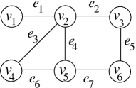
$$\begin{array}[]{l|c|c|c|c|c|c||c}s_{i,j}&j=1&j=2&j=3&j=4&j=5&j=6&c_{i}\\ \hline\cr i=1&1&1&0&0&0&0&1\\ i=2&0&1&1&0&0&0&1\\ i=3&0&1&0&1&0&0&1\\ i=4&0&1&0&0&1&0&1\\ i=5&0&0&1&0&0&1&1\\ i=6&0&0&0&1&1&0&1\\ i=7&0&0&0&0&1&1&1\\ \hline\cr\hline\cr p_{j}&1&1&1&1&1&1\\ \end{array}$$

Figure 1: Reduction in the proof of Theorem 4.4

Remark 4.6

The proof of Theorem 4.4 shows that Max d-KP is not pseudo-polynomial for $n\leq d$. In order to show the same result for the more common case $d<n$ we can consider special Max Independent Set instances by replacing every graph $G=(V,E)$ by $G^{\prime}=(V^{\prime},E)$, where $V^{\prime}=V\cup\{v_{e}~{}|~{}e\in E\}$.

Theorem 4.7

For every fixed $d$ there is a pseudo-polynomial algorithm that solves Max d-KP in time $\mathcal{O}(n\cdot d\cdot(c_{\max})^{d})$.

Proof  We consider the algorithm with running time $\mathcal{O}(n\cdot d\cdot(c_{\max})^{d})$ of Theorem 4.3. If $d$ is assumed to be fixed, $n\cdot d$ is polynomial in the input size and $(c_{\max})^{d}$ is polynomial in the value of the largest occurring number in every input. $\Box$

4.4 Parameterized Algorithms

Also the Max d-KP problem is defined on inputs of various informations, which motivates us to consider parameterized versions of the problem. By adding a threshold value $k$ for the profit to the instance and choosing a parameter $\kappa(I)$ from the instance $I$, we define the following parameterized problem.

• $\kappa$-d-dimensional Knapsack ($\kappa$-d-KP)

• A set $A=\{a_{1},\ldots,a_{n}\}$ of $n$ items and a number $d$ of dimensions. Every item $a_{j}$ has a profit $p_{j}$ and for dimension $i$ the size $s_{i,j}$. Further for every dimension $i$ there is a capacity $c_{i}$ and we have given a positive integer $k$.

• $\kappa(I)$

• Is there a subset $A^{\prime}\subseteq A$ such that the total profit of $A^{\prime}$ is at least $k$ and for every dimension $i$ the total size of $A^{\prime}$ is at most the capacity $c_{i}$?

In Theorem 7 in [33] it is shown that for $d=2$ dimensions $k$-d-KP is $\mbox{W}[1]$-hard. We generalize this result for $d\geq 2$ dimensions to obtain a result for parameter $(d,k)$ in Theorem 4.9.

Lemma 4.8

For every $d\geq 2$ problem $k$-d-KP is $\mbox{W}[1]$-hard.

Proof  Let $I$ be an instance for $k$-d-KP on $d$ dimensions and $n$ items of profits $p_{j}$ and sizes $s_{i,j}$ and $m$ knapsacks of capacities $c_{i}$. We define an instance $I^{\prime}$ for $k$-d-KP on $d+1$ dimensions and $n$ items of profits $p^{\prime}_{j}$ and sizes $s^{\prime}_{i,j}$ and $m$ knapsacks of capacities $c^{\prime}_{i}$ as follows. The profits are $p^{\prime}_{j}=p_{j}$ for $1\leq j\leq n$. The sizes are $s^{\prime}_{i,j}=s_{i,j}$ for $1\leq i\leq d$ and $1\leq j\leq n$ and $s^{\prime}_{d+1,j}=1$ for $1\leq j\leq n$. The capacities are $c^{\prime}_{i}=c_{i}$ for $1\leq i\leq d$ and $c_{d+1}=n$. Then $I$ has a solution of profit $k$ if and only if $I^{\prime}$ has a solution of profit $k$. $\Box$

Next we give parameterized algorithms for the d-dimensional knapsack problem.

Parameter	class	time
$n$	$\not\in\mbox{PFPT}$, $\in\mbox{FPT}$	$\mathcal{O}(d\cdot n\cdot 2^{n})$	$\subseteq$	$\mathcal{O}(|I|\cdot 2^{n})$
$k$	$\mbox{W}[1]$-hard, $\in\mbox{XP}$	$\mathcal{O}(d\cdot n^{k+1})$	$\subseteq$	$\mathcal{O}(|I|\cdot n^{k})$
$(c_{1},\ldots,c_{d})$	$\in\mbox{PFPT}$	$\mathcal{O}(d\cdot n\cdot\Pi_{i=1}^{d}c_{i})$	$\subseteq$	$\mathcal{O}(|I|\cdot\Pi_{i=1}^{d}c_{i})$
$(p_{1},\ldots,p_{n})$	$\in\mbox{FPT}$	$\mathcal{O}(d\cdot n\cdot 2^{(\sum_{j=1}^{n}p_{j})})$	$\subseteq$	$\mathcal{O}(|I|\cdot 2^{(\sum_{j=1}^{n}p_{j})})$
$(s_{1,1},\ldots,s_{d,n})$	$\in\mbox{FPT}$	$\mathcal{O}(d\cdot n\cdot 2^{\sum_{j=1}^{n}\sum_{i=1}^{d}s_{i,j}})$	$\subseteq$	$\mathcal{O}(|I|\cdot 2^{\sum_{j=1}^{n}\sum_{i=1}^{d}s_{i,j}})$
$d$	$\not\in\mbox{XP}$
$(d,\text{val})$	$\in\mbox{FPT}$	$\mathcal{O}(d\cdot n\cdot 2^{d\cdot\operatorname{val}(I)})$	$\subseteq$	$\mathcal{O}(|I|\cdot 2^{d\cdot\operatorname{val}(I)})$
$(d,c_{\max})$	$\in\mbox{FPT}$	$\mathcal{O}(d\cdot n\cdot(c_{\max})^{d})$	$\subseteq$	$\mathcal{O}(|I|\cdot(c_{\max})^{d})$
$(d,k)$	$\not\in\mbox{FPT}$, $\in\mbox{XP}$	$\mathcal{O}(d\cdot n^{k+1})$

Table 3: Overview of parameterized algorithms for d-KP

Theorem 4.9

There exist parameterized algorithms for the d-dimensional knapsack problem such that the running times of Table 3 hold true and the problems belong to the specified parameterized complexity classes.

Proof  For parameter $\kappa(I)=n$ we can use a brute force solution by checking for all $2^{n}$ possible subsets of $A$ within condition (7) in the given BIP, which leads to an algorithm of time complexity $\mathcal{O}(d\cdot n\cdot 2^{n})$. Alternatively one can use the result of [34] or its improved version in [30], which implies that integer linear programming is fixed-parameter tractable for the parameter ”number of variables”. Thus by BIP (6)-(8) problem $n$-d-KP is fixed-parameter tractable.

As a lower bound Corollary 2.2 implies that there is no polynomial fpt-algorithm for $n$-d-KP.

For the standard parameterization $\kappa(I)=k$ we can use the reduction given in the proof of Theorem 4.4 in order to obtain a parameterized reduction from the $k$-Independent Set problem, which is $\mbox{W}[1]$-hard, see [13]. Thus $k$-d-KP is $\mbox{W}[1]$-hard.

In order to obtain an xp-algorithm that solves $k$-d-KP we apply the result of Lemma 4.2 which allows us to assume that every solution $A^{\prime}$ of $k$-d-KP has at most $k$ items. Thus we have to check at most $n^{k}$ different possible solutions. Each such solution can be verified with condition (7) of the given BIP in time $\mathcal{O}(d\cdot n)$, which implies an xp-algorithm w.r.t. parameter $k$ of time $\mathcal{O}(d\cdot n^{k+1})$.

For parameter $\kappa(I)=(c_{1},\ldots,c_{d})$ we consider the dynamic programming algorithm cited in Theorem 4.3 which has running time $\mathcal{O}(d\cdot n\cdot\Pi_{i=1}^{d}c_{i})$. From a parameterized point of view a polynomial fpt-algorithm that solves $(c_{1},\ldots,c_{d})$-d-KP follows.

For parameter $\kappa(I)=(p_{1},\ldots,p_{n})$ we know that $n\leq\sum_{j=1}^{n}p_{j}$ since all profits are positive integers and thus we conclude an fpt-algorithm for d-KP w.r.t. $(p_{1},\ldots,p_{n})$ by the result for parameter $n$.

An xp-algorithm w.r.t. $(p_{1},\ldots,p_{n})$ can be obtained as follows. If for some $(p_{1},\ldots,p_{n})$-d-KP instance it holds $\sum_{j=1}^{n}p_{j}<k$, then it is not possible to reach a profit of $k$. Otherwise we know that $k\leq\sum_{j=1}^{n}p_{j}$ which implies by the upper result for parameter $k$ an xp-algorithm of running time $\mathcal{O}(d\cdot n^{\sum_{j=1}^{n}p_{j}+1})$ for $(p_{1},\ldots,p_{n})$-d-KP.

The parameter $\kappa(I)=(s_{1,1},\ldots,s_{d,n})$ can be treated in the same way. Since all sizes are non-negative integers and $\sum_{i=1}^{d}s_{i,j}\geq 1$ for every item $a_{j}$ by our assumptions, it holds $n\leq\sum_{j=1}^{n}\sum_{i=1}^{d}s_{i,j}$ and thus we conclude an fpt-algorithm for d-KP w.r.t. $(s_{1,1},\ldots,s_{d,n})$ by the result for parameter $n$.

If we choose $\kappa(I)=d$ then the parameterized problem is at least $\mbox{W}[1]$-hard, unless $\mbox{P}=\mbox{NP}$. An fpt-algorithm with respect to parameter $d$ would imply a polynomial time algorithm for every fixed $d$, but even for $d=1$ the problem is NP-hard. For the same reason there is no xp-algorithm with respect to parameter $d$.

Next we consider several combined parameters including $d$. For parameter $\kappa(I)=(d,\text{val})$ we apply Theorem 4.3 to obtain a parameterized running time of $\mathcal{O}(d\cdot n\cdot(c_{\max})^{d})\subseteq\mathcal{O}(d\cdot n\cdot(2^{\operatorname{val}(I)})^{d})$.

For parameter $\kappa(I)=(d,c_{\max})$ we also can use Theorem 4.3 which leads to the fact that d-KP can be solved in time $\mathcal{O}(n\cdot d\cdot(c_{\max})^{d})$.

For parameter $\kappa(I)=(d,k)$ the problem d-KP is $\mbox{W}[1]$-hard. If $(d,k)$-d-KP would be in FPT, then for every fixed dimension $d$ problem $k$-d-KP is fixed-parameter tractable in contradiction to Lemma 4.8. Since the running time $\mathcal{O}(d\cdot n^{k+1})$, which was mentioned above for parameter $k$, is polynomial for every fixed $k$ and $d$ the problem $(d,k)$-d-KP is slicewise polynomial. $\Box$

Theorem 4.9 states $\mbox{W}[1]$-hardness of $k$-d-KP. But this changes if we only look for solutions of high profit. Under a restriction $n/c\leq k$, for some constant $c>1$, fixed parameter tractability with regard to $n$ then implies the problem to be in FPT with respect to parameter $k$.

4.5 Kernelizations

Next we give kernelization bounds for the d-dimensional knapsack problem.

Parameter	lower bound	upper bound
$n$          if $d\leq n$	$\omega(1)$	$\mathcal{O}(n^{5})$
$(c_{1},\ldots,c_{d})$	$\Theta(1)$	$\Theta(1)$
$(p_{1},\ldots,p_{n})$		$\mathcal{O}(2^{(\sum_{j=1}^{n}p_{j})})$
$(s_{1,1},\ldots,s_{d,n})$		$\mathcal{O}(2^{\sum_{j=1}^{n}\sum_{i=1}^{d}s_{i,j}})$
$(d,\text{val})$		$\mathcal{O}(2^{d\cdot\operatorname{val}(I)})$
$(d,c_{\max})$		$\mathcal{O}((c_{\max})^{d})$

Table 4: Overview for kernel sizes of parameterized d-KP

Theorem 4.10

There exist kernelizations for the parameterized d-dimensional knapsack problem such that the upper bounds for the sizes of a possible kernel in Table 4 hold true.

Proof  For parameter $\kappa(I)=n$ let $I$ be an instance of $n$-d-KP. We proceed as in the proof of Theorem 3.6. In the case of $n$-d-KP we have to scale $d$ inequalities of type (4) and one inequality of type (5) by Theorem 2.9. For the obtained instance $I^{\prime}$ we can bound $|I^{\prime}|$ by the number of items $n$ and $d(n+1)+(n+1)=(d+1)(n+1)$ numbers of value at most $2^{4(n+1)^{3}}(\ell+2)^{(n+1)(n+3)}$. Since we can assume $\ell\leq n$ for d-KP, this problem has a kernel of size

$$\mathcal{O}\left(n+(d+1)(n+1)\log_{2}\left(2^{4(n+1)^{3}}(\ell+2)^{(n+1)(n+3)}\right)\right)\subseteq\mathcal{O}(d\cdot n^{4}+d\cdot\log_{2}(\ell+2)n^{3})\subseteq\mathcal{O}(d\cdot n^{4}),$$

which implies a kernel for $n$-d-KP of size $\mathcal{O}(n^{4})$ for every fixed $d$ and a kernel of size $\mathcal{O}(n^{5})$ for $d\leq n$.

For parameter $\kappa(I)=(c_{1},\ldots,c_{d})$ we obtain by Theorem 4.9 and Theorem 2.6 a kernel of constant size.

For the remaining four parameters of Table 4 the upper bounds follow by Theorem 4.9 and Theorem 2.3. $\Box$

5 Multiple Knapsack Problem

Next we consider the multiple knapsack problem.

• Max multiple Knapsack (Max MKP)

• A set $A=\{a_{1},\ldots,a_{n}\}$ of $n$ items and a number $m$ of knapsacks. Every item $a_{j}$ has a profit $p_{j}$ and a size $s_{j}$. Each knapsack $i$ has a capacity $c_{i}$.

• Find $m$ disjoint (possibly empty) subsets $A_{1},\ldots,A_{m}$ of $A$ such that the total profit of the selected items is maximized and each subset can be assigned to a different knapsack $i$ without exceeding its capacity $c_{i}$ by the sizes of the selected items.

For $m=1$ the Max MKP problem corresponds to the Max KP problem considered in Section 3. Max MKP does not allow an FPTAS even for $m=2$ knapsacks, see [8] or [5]. Max MKP allows an EPTAS of running time $2^{\mathcal{O}(\nicefrac{{1}}{{\epsilon}}\cdot\log^{4}(\nicefrac{{1}}{{\epsilon}}))}+n^{\mathcal{O}(1)}$, see [28].

The parameters $n$, $m$, $p_{j}$, $s_{j}$, and $c_{i}$ are assumed to be positive integers. Let $s_{\max}=\max_{1\leq j\leq n}s_{j}$, $p_{\max}=\max_{1\leq j\leq n}p_{j}$, and $c_{\max}=\max_{1\leq i\leq m}c_{i}$. The same notations are also used for $\min$ instead of $\max$. In order to avoid trivial solutions we assume that $s_{\max}\leq c_{\max}$, $s_{\min}\leq c_{\min}$, and $\sum_{j=1}^{n}s_{j}>c_{\max}$. Further we can assume that $n\geq m$, since otherwise we can eliminate the $m-n$ knapsacks of smallest capacity.

For some instance $I$ of Max MKP its size $|I|$ can be bounded (cf. [21]) by

$$\begin{array}[]{lcl}|I|&=&n+\sum_{j=1}^{n}(1+\lfloor\log_{2}(p_{j})\rfloor)+\sum_{j=1}^{n}(1+\lfloor\log_{2}(s_{j})\rfloor)+\sum_{i=1}^{m}(1+\lfloor\log_{2}(c_{i})\rfloor)\\ &\in&\mathcal{O}(n+m+\sum_{j=1}^{n}\log_{2}(p_{j})+\sum_{j=1}^{n}\log_{2}(s_{j})+\sum_{i=1}^{m}\log_{2}(c_{i}))\\ &=&\mathcal{O}(n+m+n\cdot\log_{2}(p_{\max})+n\cdot\log_{2}(s_{\max})+m\cdot\log_{2}(c_{\max})).\\ \end{array}$$

By assuming that we have one knapsack of capacity $\sum_{i=1}^{m}c_{i}$ similar as in the poof of Lemma 3.1 we can bound the number of items w.r.t. the sum of all capacities.

Lemma 5.1 (Reduced Instance)

Every instance of Max MKP can be transformed into a reduced instance, such that $n\in\mathcal{O}(\log(c_{\max})\cdot\sum_{i=1}^{m}c_{i})$.

Proof  First we can assume, that there is no item in $A$, whose size is larger than the maximum capacity $c_{\max}$, i.e. $s_{j}\leq c_{\max}$ for every $1\leq j\leq n$. Further for $1\leq s\leq c_{\max}$ we can assume that there are at most $n_{s}:=\lfloor\frac{\sum_{i=1}^{m}c_{i}}{s}\rfloor$ items of size $s$ in $A$.

By the harmonic series we always can bound the number $n$ of items in $A$ by

$$\begin{array}[]{lcl}n&\leq&\sum_{s=1}^{c_{\max}}n_{s}\\ &=&\sum_{s=1}^{c_{\max}}\bigg{\lfloor}\frac{\sum_{i=1}^{m}c_{i}}{s}\bigg{\rfloor}\\ &\leq&\sum_{s=1}^{c_{\max}}\frac{\sum_{i=1}^{m}c_{i}}{s}\\ &=&(\sum_{i=1}^{m}c_{i})\cdot\sum_{s=1}^{c_{\max}}\frac{1}{s}\\ &<&(\sum_{i=1}^{m}c_{i})\cdot(\ln(c_{\max})+1)\\ &\in&\mathcal{O}((\sum_{i=1}^{m}c_{i})\cdot\log(c_{\max})).\end{array}$$

If we have given an instance $I_{1}$ for Max MKP with more than the mentioned number $n_{s}$ of items of size $s$ for some $1\leq s\leq c_{\max}$, we remove all of them except the $n_{s}$ items of the highest profit. The new instance $I_{2}$ satisfies $n\in\mathcal{O}(\log(c_{\max})\cdot\sum_{i=1}^{m}c_{i})$ and is a reduced instance of $I_{1}$. $\Box$

Lemma 5.2 (Bounding the size of a solution)

For every instance of Max MKP there is a feasible solution $A_{1},\ldots,A_{m}$ of profit at least $k$ if and only if there is a feasible solution $A^{\prime}_{1},\ldots,A^{\prime}_{m}$ of profit at least $k$, which has size at most $k$.

Proof  If $|A_{1}\cup\ldots\cup A_{m}|\geq k+1$ we can remove one item of smallest profit, since all profits are positive integers. $\Box$

5.1 Binary Integer Programming

By choosing a boolean variable $x_{i,j}$ for every item $a_{j}\in A$ and every knapsack $1\leq i\leq m$, indicating whether or not the item $a_{j}$ will be put into knapsack $i$, a binary integer programming (BIP) version of the Max MKP problem is as follows.

max $$\sum_{i=1}^{m}\sum_{j=1}^{n}p_{j}\cdot x_{i,j}$$ (9)

s.t. $$\sum_{j=1}^{n}s_{j}\cdot x_{i,j}\leq c_{i}\text{ for }i\in[m]$$ (10)

and $$\sum_{i=1}^{m}x_{i,j}\leq 1\text{ for }j\in[n]$$ (11)

and $$x_{i,j}\in\{0,1\}\text{ for }i\in[m],j\in[n]$$ (12)

The condition (11) ensures that all knapsacks are disjoint, i.e. every item is contained in at most one knapsack.

5.2 Dynamic Programming Algorithms

A dynamic programming solution for Max MKP for $m=2$ knapsacks can be found in [42], which can be generalized as follows.

Theorem 5.3

Max MKP can be solved in time $\mathcal{O}(n\cdot m\cdot\prod_{i=1}^{m}c_{i})\subseteq\mathcal{O}(n\cdot m\cdot(c_{\max})^{m})$

Proof  We define $P[k,c^{\prime}_{1},\ldots,c^{\prime}_{m}]$ to be the maximum profit of the subproblem where we only may choose a subset from the first $k$ items $a_{1},\ldots,a_{k}$ and the capacities are $c^{\prime}_{1},\ldots,c^{\prime}_{m}$. We initialize $P[0,c^{\prime}_{1},\ldots,c^{\prime}_{m}]=0$ for all $c^{\prime}_{1},\ldots,c^{\prime}_{m}$ since when choosing none of the items, the profit is always zero. Further we set $P[k,c^{\prime}_{1},\ldots,c^{\prime}_{m}]=-\infty$ if at least one of the $c^{\prime}_{1},\ldots,c^{\prime}_{m}$ is negative in order to represent the case where the size $s_{k}$ of an item is too high for packing it into a knapsack of capacity $c^{\prime}_{i}$. The values $P[k,c^{\prime}_{1},\ldots,c^{\prime}_{m}]$, $1\leq k\leq n$, for every $0\leq c^{\prime}_{i}\leq c_{i}$ and every $1\leq i\leq m$ can be computed by the following recursion.

$$P[k,c^{\prime}_{1},\ldots,c^{\prime}_{m}]=\max\left\{\begin{array}[]{lll}P[k-1,c^{\prime}_{1},\ldots,c^{\prime}_{m}]\\ P[k-1,c^{\prime}_{1}-s_{k},\ldots,c^{\prime}_{m}]+p_{k}\\ $\vdots$\\ P[k-1,c^{\prime}_{1},\ldots,c^{\prime}_{m}-s_{k}]+p_{k}\\ \end{array}\right.$$

All these values define a table with $\mathcal{O}(n\cdot\prod_{i=1}^{m}c_{i})$ fields, where each field can be computed in time $\mathcal{O}(m)$. The optimal return is $P[n,c_{1},\ldots,c_{m}]$. Thus we have shown that Max MKP can be solved in time $\mathcal{O}(n\cdot m\cdot\prod_{i=1}^{m}c_{i})$. $\Box$

5.3 Pseudo-polynomial Algorithms

The existence of pseudo-polynomial algorithms for Max MKP depends on the assumption whether the number of knapsacks $m$ is given in the input or is assumed to be fixed.

Theorem 5.4

Max MKP is not pseudo-polynomial.

Proof  We give a pseudo-polynomial reduction (cf. page 101 in [21]) from 3-Partition which is not pseudo-polynomial by [21]. Given are $n=3m$ positive integers $w_{1},\ldots,w_{n}$ such that the sum $\frac{1}{m}\cdot\sum_{j=1}^{n}w_{j}=B$ and $\nicefrac{{B}}{{4}}<w_{j}<\nicefrac{{B}}{{2}}$ for every $1\leq j\leq n$. The question is to decide whether there is a partition of $N=\{1,\ldots,n\}$ into $m$ sets $N_{1},\ldots,N_{m}$ such that $\sum_{j\in N_{i}}w_{j}=B$ for every $1\leq i\leq m$.

Let $I$ be an instance for the 3-Partition. We define an instance $I^{\prime}$ for Max MKP by choosing the number of items as $n$, the number of knapsacks as $m$, the capacities $c_{i}=B$ for $1\leq i\leq m$, the profits $p_{j}=1$ and sizes $s_{j}=w_{j}$ for $1\leq j\leq n$. By this construction every 3-Partition solution for $I$ implies a solution with optimal profit $n$ for the Max MKP instance $I^{\prime}$ and vice versa. $\Box$

Theorem 5.5

For every fixed $m$ there is a pseudo-polynomial algorithm that solves Max MKP in time $\mathcal{O}(n\cdot m\cdot(c_{\max})^{m})$.

Proof  We consider the algorithm with running time $\mathcal{O}(n\cdot m\cdot(c_{\max})^{m})$ of Theorem 5.3. If $m$ is assumed to be fixed, $n\cdot m$ is polynomial in the input size and $(c_{\max})^{m}$ is polynomial in the value of the largest occurring number in every input. $\Box$

5.4 Parameterized Algorithms

Also the Max MKP problem is defined on inputs of various informations, which motivates us to consider parameterized versions of the problem. By adding a threshold value $k$ for the profit to the instance and choosing a parameter $\kappa(I)$ from the instance $I$, we define the following parameterized problem.

• $\kappa$-multiple Knapsack ($\kappa$-MKP)

• A set $A=\{a_{1},\ldots,a_{n}\}$ of $n$ items and a number $m$ of knapsacks. Every item $a_{j}$ has a profit $p_{j}$ and a size $s_{j}$. Each knapsack $i$ has a capacity $c_{i}$ and we have given a positive integer $k$.

• $\kappa(I)$

• Are there $m$ disjoint (possibly empty) subsets $A_{1},\ldots,A_{m}$ of $A$ such that the total profit of the selected items is at least $k$ and each subset can be assigned to a different knapsack $i$ without exceeding its capacity $c_{i}$ by the sizes of the selected items?

We give a bound on the number of items in the threshold value for the profit $k$.

Lemma 5.6 (Reduced Instance)

Every instance of Max MKP can be transformed into a reduced instance, such that $n\in\mathcal{O}(k\cdot\log(k))$.

Proof  For some fixed profit $p$, $p\geq 1$ we need at most $\lceil\frac{k}{p}\rceil$ many items of profit $p$ in order to reach the profit $k$. If we have given an instance for Max MKP with more than $\lceil\frac{k}{p}\rceil$ items of profit $p$, we remove all of them except the $\lceil\frac{k}{p}\rceil$ items of the smallest size. Since each profit is a positive integer we can bound the number of items by $n\leq\sum_{p=1}^{\infty}\lceil\frac{k}{p}\rceil$. Further all items with profit $p\geq k$ can be replaced by one of them of the smallest size. Thus we can assume that $n\leq\sum_{p=1}^{k}\lceil\frac{k}{p}\rceil$. Further by the harmonic series it holds

$$n\leq\sum_{p=1}^{k}\bigg{\lceil}\frac{k}{p}\bigg{\rceil}\leq\sum_{p=1}^{k}\bigg{(}\frac{k}{p}+1\bigg{)}=k+\sum_{p=1}^{k}\frac{k}{p}=k+k\cdot\sum_{p=1}^{k}\frac{1}{p}<k+k\cdot(\ln(k)+1)\in\mathcal{O}(k\cdot\log(k)).$$

$\Box$

Next we give parameterized algorithms for the multiple knapsack problem. Therefor let $B(n)=\sum_{i=0}^{n-1}\binom{n-1}{i}B(i)$ be the $n$-th Bell number which asymptotically grows faster than $c^{n}$ for every constant $c$ but slower than $n$ factorial.

Parameter	class	time
$n$	$\not\in\mbox{PFPT}$, $\in\mbox{FPT}$	$\mathcal{O}(B(n)\cdot(m\cdot\log(m)+n))$	$\subseteq$	$\mathcal{O}(|I|^{2}\cdot B(n))$
$k$	$\in\mbox{FPT}$	$\mathcal{O}((m\cdot\log(m)+n)\cdot 2^{k\cdot\ln^{2}(k)})$	$\subseteq$	$\mathcal{O}(|I|^{2}\cdot 2^{k\cdot\ln^{2}(k)})$
$(c_{1},\ldots,c_{m})$	$\in\mbox{PFPT}$	$\mathcal{O}(n\cdot m\cdot\prod_{i=1}^{m}c_{i})$	$\subseteq$	$\mathcal{O}(|I|^{2}\cdot\prod_{i=1}^{m}c_{i})$
$(p_{1},\ldots,p_{n})$	$\in\mbox{FPT}$	$\mathcal{O}(B(\sum_{j=1}^{n}p_{j})\cdot(m\cdot\log(m)+n))$	$\subseteq$	$\mathcal{O}(|I|^{2}\cdot B(\sum_{j=1}^{n}p_{j}))$
$(s_{1},\ldots,s_{n})$	$\in\mbox{FPT}$	$\mathcal{O}(B(\sum_{j=1}^{n}s_{j})\cdot(m\cdot\log(m)+n))$	$\subseteq$	$\mathcal{O}(|I|^{2}\cdot B(\sum_{j=1}^{n}s_{j}))$
$m$	$\not\in\mbox{XP}$
$(m,\text{val})$	$\in\mbox{FPT}$	$\mathcal{O}(n\cdot m\cdot 2^{m\cdot\operatorname{val}(I)})$	$\subseteq$	$\mathcal{O}(|I|^{2}\cdot 2^{m\cdot\operatorname{val}(I)})$
$(m,c_{\max})$	$\in\mbox{FPT}$	$\mathcal{O}(n\cdot m\cdot(c_{\max})^{m})$	$\subseteq$	$\mathcal{O}(|I|^{2}\cdot(c_{\max})^{m})$
$(m,n)$	$\in\mbox{FPT}$	$\mathcal{O}(n\cdot m\cdot 2^{n\cdot m})$	$\subseteq$	$\mathcal{O}(|I|^{2}\cdot 2^{n\cdot m})$

Table 5: Overview for parameterized algorithms for MKP

Theorem 5.7

There exist parameterized algorithms for the multiple knapsack problem such that the running times of Table 5 hold true and the problems belong to the specified parameterized complexity classes.

Proof  We start with parameter $\kappa(I)=n$. A brute force solution to solve $n$-MKP is to consider all $B(n)$ possible partitions of the $n$ items into disjoint non-empty subsets, which all can be generated in time $\mathcal{O}(B(n))$ by [31]. For every such partition we check if it consists of at most $m$ sets and after sorting descending w.r.t. the sum of sizes in each set $A^{\prime}_{j}$ of the partition, we compare this sum with the capacity $c_{j}$. The capacities are also assumed to be sorted, such that $c_{1}\geq c_{2}\geq\ldots\geq c_{m}$. Every of these partitions can be handled in time $\mathcal{O}(m\cdot\log(m)+n)$ for sorting the sets $A^{\prime}_{j}$ and summing up the sizes. This leads to an fpt-algorithm that solves $n$-MKP in time $\mathcal{O}(B(n)\cdot(m\cdot\log(m)+n))$.

As a lower bound Corollary 2.2 implies that there is no polynomial fpt-algorithm for $n$-MKP.

For parameter $\kappa(I)=k$ by the result for parameter $n$ and Lemma 5.6 we obtain an fpt-algorithm that solves $k$-MKP in time $\mathcal{O}(B(k\cdot\ln(k))\cdot(m\cdot\log(m)+n))$. By the bound on the Bell number $B(\ell)\leq(\frac{\ell}{\ln(\ell)})^{\ell}$ shown in [2] we obtain the following inclusions.

$$\begin{array}[]{lcl}\mathcal{O}((\frac{k\cdot\ln(k)}{\ln(k\cdot\ln(k))})^{k\cdot\ln(k)}\cdot(m\cdot\log(m)+n))&\subseteq&\mathcal{O}(k^{k\cdot\ln(k)}\cdot(m\cdot\log(m)+n))\\ &\subseteq&\mathcal{O}(2^{k\cdot\ln^{2}(k)}\cdot(m\cdot\log(m)+n))\end{array}$$

Thus there is an fpt-algorithm that solves $k$-MKP in time $\mathcal{O}(2^{k\cdot\ln^{2}(k)}\cdot(m\cdot\log(m)+n))\subseteq\mathcal{O}(2^{k\cdot\ln^{2}(k)}\cdot n^{2})$.

For parameter $\kappa(I)=(c_{1},\ldots,c_{m})$ we use the running time mentioned in Theorem 5.3 to obtain a polynomial fpt-algorithm that solves $(c_{1},\ldots,c_{m})$-MKP in time $\mathcal{O}(n\cdot m\cdot\prod_{i=1}^{m}c_{i})$.

For parameter $\kappa(I)=(p_{1},\ldots,p_{n})$ we know that $n\leq\sum_{j=1}^{n}p_{j}$ since all profits are positive integers and thus we conclude an fpt-algorithm of running time $\mathcal{O}(B(\sum_{j=1}^{n}p_{j})\cdot(m\cdot\log(m)+n))$ for MKP w.r.t. $(p_{1},\ldots,p_{n})$ by the result for parameter $n$.

For parameter $\kappa(I)=(s_{1},\ldots,s_{n})$ we know that $n\leq\sum_{j=1}^{n}s_{j}$ since all sizes are positive integers and in the same way as for the profits we conclude an fpt-algorithm for MKP w.r.t. $(s_{1},\ldots,s_{n})$.

If we choose $\kappa(I)=m$ the parameterized problem is at least $\mbox{W}[1]$-hard, unless $\mbox{P}=\mbox{NP}$. An fpt-algorithm with respect to parameter $m$ would imply a polynomial time algorithm for every fixed $m$, but even for $m=1$ the problem is NP-hard. For the same reason there is no xp-algorithm with respect to parameter $m$.

Next we consider several combined parameters including $m$. For parameter $\kappa(I)=(m,\text{val})$ we apply Theorem 5.3 to obtain a parameterized running time of $\mathcal{O}(n\cdot m\cdot(c_{\max})^{m})\subseteq\mathcal{O}(n\cdot m\cdot(2^{\operatorname{val}(I)})^{m})\subseteq\mathcal{O}(n\cdot m\cdot 2^{m\cdot\operatorname{val}(I)})$. Thus there is an fpt-algorithm that solves $(m,\text{val})$-MKP in time $\mathcal{O}(n\cdot m\cdot 2^{m\cdot\operatorname{val}(I)})$.

For parameter $\kappa(I)=(m,c_{\max})$ we also use Theorem 5.3 to show that the $(m,c_{\max})$-MKP problem is fixed-parameter tractable with running time $\mathcal{O}(n\cdot m\cdot(c_{\max})^{m})$

Finally for the parameter $\kappa(I)=(m,n)$ we verify all possible $2^{n\cdot m}$ assignments of the $n\cdot m$ variables in (9)-(12) each in time $\mathcal{O}(n\cdot m)$. Thus there is an fpt-algorithm that solves $(m,n)$-MKP in time $\mathcal{O}(n\cdot m\cdot 2^{n\cdot m})$.

Alternatively we can apply the result of [30], which implies that integer linear programming is fixed-parameter tractable for the parameter ”number of variables”. By BIP (9)-(12) for Max MKP we obtain an fpt-algorithm that solves $(m,n)$-MKP in time $\mathcal{O}((n\cdot m)^{\mathcal{O}(n\cdot m)}\cdot|I|)$. $\Box$

Next we give some further ideas how to show parameterized algorithms for $k$-MKP. Although these are less efficient, the ideas might be interesting on its own.

Remark 5.8

1. The Max MKP problem allows an EPTAS of parameterized running time $2^{\mathcal{O}(\nicefrac{{1}}{{\epsilon}}\cdot\log^{4}(\nicefrac{{1}}{{\epsilon}}))}+n^{\mathcal{O}(1)}$, see [28]. By Theorem 2.10 we can use this EPTAS for $\epsilon=\nicefrac{{1}}{{2k}}$ in order to obtain an fpt-algorithm that solves the standard parameterization of the corresponding decision problem in time $2^{\mathcal{O}(k\cdot\log^{4}(k))}+n^{\mathcal{O}(1)}$. Thus there is an fpt-algorithm that solves $k$-MKP in time $2^{\mathcal{O}(k\cdot\log^{4}(k))}+n^{\mathcal{O}(1)}$.

2. By Lemma 5.2 we can restrict to solutions which have size at most $k$. Formally we need to bound the number of families of disjoint subsets $A^{\prime}_{1},\ldots,A^{\prime}_{m}$ of a set $A$ on $n$ elements, such that $|A^{\prime}_{1}\cup\ldots\cup A^{\prime}_{m}|\leq k$. Thus for $1\leq i\leq k$ we sum up $B(i)$ multiplicated by $\binom{n}{i}$ possible ways to choose the $i$ items from all $n$ items.

   $$\begin{array}[]{lcll}\sum_{i=1}^{k}\binom{n}{i}B(i)&=&\sum_{i=1}^{k}\binom{k}{i}\frac{(k-i)!n!}{k!(n-i)!}B(i)&\text{since }\frac{\binom{n}{i}}{\binom{k}{i}}=\frac{(k-i)!n!}{k!(n-i)!}\\ &\leq&\frac{n!}{(n-k)!}\sum_{i=1}^{k}\binom{k}{i}B(i)&\text{since }i\leq k\\ &\leq&\frac{n!}{(n-k)!}B(k+1)&\text{by definition of }B(k+1)\\ &\leq&n^{k}B(k+1)&\text{since }\frac{n!}{(n-k)!}\leq n^{k}\end{array}$$

   Every of these partitions can be generated in constant time by [31] and handled in time $\mathcal{O}(m\cdot\log(m)+n)$ as mentioned in the proof of Theorem 5.7. Thus there is an xp-algorithm that solves $k$-MKP in time $\mathcal{O}(n^{k}\cdot B(k+1)\cdot(m\cdot\log(m)+n))\subseteq\mathcal{O}(n^{k+2}\cdot B(k+1))$.

5.5 Kernelizations

Next we give kernelization bounds for the multiple knapsack problem.

Parameter	lower bound	upper bound
$n$	$\omega(1)$	$\mathcal{O}(n^{8})$
$k$		$\mathcal{O}(2^{k\cdot\ln^{2}(k)})$
$(c_{1},\ldots,c_{m})$	$\Theta(1)$	$\Theta(1)$
$(p_{1},\ldots,p_{n})$		$\mathcal{O}(B(\sum_{j=1}^{n}p_{j}))$
$(s_{1},\ldots,s_{n})$		$\mathcal{O}(B(\sum_{j=1}^{n}s_{j}))$
$(m,\text{val})$		$\mathcal{O}(2^{m\cdot\operatorname{val}(I)})$
$(m,c_{\max})$		$\mathcal{O}((c_{\max})^{m})$
$(m,n)$		$\mathcal{O}(2^{n\cdot m})$

Table 6: Overview for kernel sizes of parameterized MKP

Theorem 5.9

There exist kernelizations for the parameterized multiple knapsack problem such that the upper bounds for the sizes of a possible kernel in Table 6 hold true.

Proof  For parameter $\kappa(I)=n$ we proceed as in the proof of Theorem 3.6 which shows a kernel of size $\mathcal{O}(n^{4})$ for $n$-KP. In the case of $n$-MKP we have to scale $m$ inequalities of type (4) on $n$ variables and one inequality of type (5) on $n\cdot m$ variables by Theorem 2.9. For the obtained instance $I^{\prime}$ we can bound $|I^{\prime}|$ by the number of items $n$ and $m(n+1)$ numbers of value at most $2^{4(n+1)^{3}}(\ell+2)^{(n+1)(n+3)}$ and $n\cdot m+1$ numbers of value at most $2^{4(nm+1)^{3}}(\ell+2)^{(nm+1)(nm+3)}$. Thus $n$-MKP has a kernel of size

$$\mathcal{O}\left(n+m(n+1)\log_{2}(2^{4(n+1)^{3}}(\ell+2)^{(n+1)(n+3)})+(nm+1)\log_{2}(2^{4(nm+1)^{3}}(\ell+2)^{(nm+1)(nm+3)})\right).$$

We can assume $m\leq n$ (cf. beginning of Section 5) and since every item is assigned to at most one knapsack (cf. (11)) we know $\ell\leq n$. Thus we obtain a kernel of size

$$\mathcal{O}(n\cdot m\cdot n^{3}+n\cdot m\cdot\log_{2}(\ell+2)n^{2}+n\cdot m\cdot(nm)^{3}+n\cdot m\cdot\log_{2}(\ell+2)(nm)^{2})\subseteq\mathcal{O}(n^{4}\cdot m^{4})\subseteq\mathcal{O}(n^{8}).$$

for $n$-MKP.

For parameter $\kappa(I)=(c_{1},\ldots,c_{m})$ we obtain by Theorem 5.7 and Theorem 2.6 a kernel of constant size.

For the remaining six parameters of Table 6 the upper bounds follow by Theorem 5.7 and Theorem 2.3. $\Box$

6 Conclusions and Outlook

We have considered the Max Knapsack problem and its two generalizations Max Multidimensional Knapsack and Max Multiple Knapsack. The parameterized decision versions of all three problems allow several parameterized algorithms.

From a practical point of view choosing the standard parameterization $k$ is not very useful, since a large profit of the subset $A^{\prime}$ violates the aim that a good parameterization is small for every input. So for KP we suggest it is better to choose the capacity as a parameter, i.e. $\kappa(I)=c$, since common values of $c$ are low enough such that the polynomial fpt-algorithm is practical. The same holds for d-KP and MKP. Further one has a good parameter, if it is smaller than the input size $|I|$ but measures the structure of the instance. This is the case for the parameter number of items $n$ within all three considered knapsack problems.

The special case of the Max Knapsack problem, where $s_{j}=p_{j}$ for all items $1\leq j\leq n$ is known as the Subset Sum problem. For this case we know that $s_{\max}=p_{\max}\leq c$ and we conclude the existence of fpt-algorithms with respect to parameter $n$, $c$, and $k$. Kernels for the Subset Sum problem w.r.t. $n$ and the number of different sizes size-var are examined in [14].

The closely related minimization problem

$$\text{min }\sum_{i=1}^{n}x_{i}\text{~{}~{} s.t. ~{}~{}}\sum_{i=1}^{n}c_{i}x_{i}=c\text{~{}~{} and ~{}~{}}x_{i}\in\{0,1\}\text{ for }i\in[n]$$ (13)

is known as the Change Making problem, whose parameterized complexity is discussed in [22].

In our future work, we want to find better fpt-algorithms, especially for d-KP and MKP. We also want to consider the following additional parameters.

• $\text{profit-var}(I)=|\{p_{1},\ldots,p_{n}\}|$ for KP

• $\text{profit-var}(I)=|\{p_{1},\ldots,p_{n}\}|$, $\text{size-var}(I)=|\{s_{1,1},\ldots,s_{d,n}\}|$, $c_{\max}$, $p_{\max}$, $s_{\max}$, and val for d-KP, and

• $\text{size-var}(I)=|\{s_{1},\ldots,s_{n}\}|$, $\text{profit-var}(I)=|\{p_{1},\ldots,p_{n}\}|$, val, $c_{\max}$, $p_{\max}$, and $s_{\max}$ for MKP.

Also from a theoretical point of view it is interesting to increase the number of parameters for which the parameterized complexity of the considered problems is known. For example if our problem is $\mbox{W}[1]$-hard with respect to some parameter $\kappa$, then a natural question is to ask, whether it remains hard for the dual parameter $\kappa_{d}(I)=\max_{I^{\prime}\in{\cal I}}\kappa(I^{\prime})-\kappa(I)$. That is, if $\kappa$ measures the costs of a solution, then for some optimization problem the dual parameter $\kappa_{d}$ measures the costs of the elements that are not in the solution [41]. Since $k$-d-KP is $\mbox{W}[1]$-hard the question arises, whether d-KP becomes tractable w.r.t. parameter $n\cdot p_{\max}-k$. More general, one also might consider more combined parameters, i.e. parameters that consists of two or more parts of the input. For d-KP combined parameters including $k$ are of our interest.

The existence of polynomial kernels for knapsack problems seems to be nearly uninvestigated. Recently a polynomial kernel for KP using rational sizes and profits is constructed in [14, 15] by Theorem 2.9. This result also holds for integer sizes and profits (cf. Theorem 3.6). By considering polynomial fpt-algorithms we could show some lower bounds for kernels for KP (cf. Table 2). We want to consider further kernels for d-KP and MKP, try to improve the sizes of known kernels, and give lower bounds for the sizes of kernels.

A further task is to extend the results to more knapsack problems, e.g. Max-Min Knapsack problem and restricted versions of the presented problems, e.g. Multiple Knapsack with identical capacities (MKP-I), see [32].

We also want to consider the existence of parameterized approximation algorithms for knapsack problems, see [38] for a survey.

References

- [1] G. Ausiello, P. Crescenzi, G. Gambosi, V. Kann, A. Marchetti-Spaccamela, and M. Protasi. Complexity and Approximation: Combinatorial Optimization Problems and Their Approximability Properties. Springer-Verlag, Berlin, 1999.
- [2] D. Berend and T. Tassa. Improved bounds on bell numbers and on moments of sums of random variables. Probability and Mathematical Statistics, 3(2), 2010.
- [3] H.L. Bodlaender. Kernelization: New Upper and Lower Bound Techniques. In Proceedings of Parameterized and Exact Computation, volume 5917 of LNCS, pages 17–37. Springer-Verlag, 2009.
- [4] L. Cai and J. Chen. On fixed-parameter tractability and approximability of NP optimization problems. Journal of Computer and System Sciences, 54:465–474, 1997.
- [5] A. Caprara, H. Kellerer, and U. Pferschy. The multiple subset sum problem. SIAM Journal of Optimization, 11:308–319, 2000.
- [6] A. Caprara, H. Kellerer, U. Pferschy, and D. Pisinger. Approximation algorithms for knapsack problems with cardinality constraints. European Journal of Operational Research, 123:333–345, 2000.
- [7] M. Cesati and L. Trevisan. On the efficiency of polynomial time approximation schemes. Inf. Process. Lett., 64(4):165–171, 1997.
- [8] C. Chekuri and S. Khanna. A PTAS for the multiple knapsack problem. In Proceedings of the ACM-SIAM Symposium on Discrete Algorithms, pages 713–728. ACM-SIAM, 2000.
- [9] J. Chena, X. Huang, I.A. Kanj, and G. Xia. Polynomial time approximation schemes and parameterized complexity. Discrete Applied Mathematics, 155(2):180–193, 2007.
- [10] G. Cornuejols and R. Tütüncü. Optimization Methods in Finance. Cambridge University Press, New York, 2013.
- [11] M. Cygan, F.V. Fomin, L. Kowalik, D. Lokshtanov, D. Marx, M. Pilipczuk, M. Pilipczuk, and S. Saurabh. Parameterized Algorithms. Springer-Verlag, New York, 2015.
- [12] R.G. Downey and M.R. Fellows. Parameterized Complexity. Springer-Verlag, New York, 1999.
- [13] R.G. Downey and M.R. Fellows. Fundamentals of Parameterized Complexity. Springer-Verlag, New York, 2013.
- [14] M. Etscheid, S. Kratsch, M. Mnich, and Röglin. Polynomial kernels for weighted problems. In Proceedings of Mathematical Foundations of Computer Science, volume 9235 of LNCS, pages 287–298. Springer-Verlag, 2015.
- [15] M. Etscheid, S. Kratsch, M. Mnich, and Röglin. Polynomial kernels for weighted problems. Journal of Computer and System Sciences, 2016. to appear.
- [16] M.R. Fellows, S. Gaspers, and F.A. Rosamond. Parameterizing by the number of numbers. In Proceedings of the Symposium on Parameterized and Exact Computation, volume 6478 of Lecture Notes in Computer Science, pages 123–134. Springer-Verlag, 2010.
- [17] H. Fernau. Parameterized Algorithmics: A Graph-Theoretic Approach. Habilitationsschrift, Universität Tübingen, Germany, 2005.
- [18] J. Flum and M. Grohe. Parameterized Complexity Theory. Springer-Verlag, Berlin, 2006.
- [19] A. Frank and E. Tardos. An application of simultaneous diophantine approximation in combinatorial optimization. Combinatorica, 7(1):49–65, 1987.
- [20] A. Fréville. The multidimensional 0-1 knapsack problem: An overview. European Journal of Operational Research, 155:1–21, 2004.
- [21] M.R. Garey and D.S. Johnson. Computers and Intractability: A Guide to the Theory of NP-Completeness. W.H. Freeman and Company, San Francisco, 1979.
- [22] St.J. Goebbels, F. Gurski, J. Rethmann, and E. Yilmaz. Fixed-parameter tractability of change-making problems (Abstract). International Conference on Operations Research (OR 2015), 2015.
- [23] F. Gurski, J. Rethmann, and E. Yilmaz. Capital budgeting problems: A parameterized point of view. In Operations Research Proceedings (OR 2014), Selected Papers, pages 205–211. Springer-Verlag, 2016.
- [24] F. Gurski, J. Rethmann, and E. Yilmaz. Computing partitions with applications to capital budgeting problems. In Operations Research Proceedings (OR 2015), Selected Papers. Springer-Verlag, 2016. to appear.
- [25] J. Hromkovic. Algorithmics for Hard Problems: Introduction to Combinatorial Optimization, Randomization, Approximation, and Heuristics. Springer-Verlag, Berlin, 2004.
- [26] O.H. Ibarra and C.E. Kim. Fast approximation algorithms for the knapsack and sum of subset problem. Journal of the ACM, 22(4):463–468, 1975.
- [27] R. Impagliazzo, R. Paturi, and F. Zane. Which problems have strongly exponential complexity? Journal of Computer and System Sciences, 63(4):512–530, 2001.
- [28] K. Jansen. A fast approximation scheme for the multiple knapsack problem. In Proceedings of the Conference on Current Trends in Theory and Practice of Computer Science, volume 7147 of LNCS, pages 313–324. Springer-Verlag, 2012.
- [29] M. Jünger, T.M. Liebling, D. Naddef, G.L. Nemhauser, W.R. Pulleyblank, G. Reinelt, G. Rinaldi, and L.A. Wolsey, editors. 50 Years of Integer Programming 1958-2008. Springer-Verlag, 2010.
- [30] R. Kannan. Minkowski’s convex body theorem and integer programming. Mathematics of Operations Research, 12:415–440, 1987.
- [31] S.-I. Kawano and S.-I. Nakano. Constant time generation of set partitions. IEICE Trans. Fundam. Electron. Commun. Comput. Sci., E88-A(4):930–934, 2005.
- [32] H. Kellerer, U. Pferschy, and D. Pisinger. Knapsack Problems. Springer-Verlag, Berlin, 2010.
- [33] A. Kulik and H. Shachnai. There is no EPTAS for two-dimensional knapsack. Information Processing Letters, 110(16):707–710, 2010.
- [34] H.W. Lenstra. Integer programming with a fixed number of variables. Mathematics of Operations Research, 8:538–548, 1983.
- [35] J. Lorie and L.J. Savage. Three problems in capital rationing. The Journal of Business, 28:229–239, 1955.
- [36] A.S. Manne and H.M. Markowitz. On the solution of discrete programming problems. Econometrica, 25:84–110, 1957.
- [37] S. Martello and P. Toth. Knapsack Problems. John Wiley & Sons, New York, 1990.
- [38] D. Marx. Parameterized complexity and approximation algorithms. The Computer Journal, 51(1):60–78, 2008.
- [39] J. Nederlof, E. J. van Leeuwen, and R. van der Zwaan. Reducing a target interval to a few exact queries. In Proceedings of Mathematical Foundations of Computer Science, volume 7464 of LNCS, pages 718–727. Springer-Verlag, 2012.
- [40] R. Niedermeier. Invitation to Fixed-Parameter Algorithms. Oxford University Press, New York, 2006.
- [41] R. Niedermeier. Reflections on multivariate algorithmics and problem parameterization. In Proceedings of the Annual Symposium of Theoretical Aspects of Computer Science, volume 5 of LIPIcs, pages 17–32. Schloss Dagstuhl - Leibniz-Zentrum fuer Informatik, 2010.
- [42] D. Pisinger and P. Toth. Knapsack problems. In Handbook of Combinatorial Optimization, volume A, pages 299–428. Kluwer Academic Publishers, 1999.
- [43] M.J. Varnamkhasti. Overview of the algorithms for solving the multidimensional knapsack problems. Advanced Studies in Biology, 4:37–47, 2012.
- [44] I. Wegener. Complexity Theory. Springer-Verlag, Berlin, 2005.
- [45] H.M. Weingartner. Capital budgeting of interrelated projects: Survey and synthesis. Management Science, 12(7):485–516, 1966.
- [46] H.M. Weingartner and D.N. Ness. Methods for the solution of the multidimensional 0/1 knapsack problem. Operations Research, 15(1):83–103, 1967.