Conservative discretization of the Landau collision integral

Abstract

We describe a density-, momentum-, and energy-conserving discretization of the nonlinear Landau collision integral. The method is suitable for both the finite-element and discontinuous Galerkin methods and does not require structured meshes. The conservation laws for the discretization are proven algebraically and demonstrated numerically for an axially symmetric nonlinear relaxation problem using a finite-element implementation.

I Introduction

Structure preserving numerical methods, which preserve a property or structure of the equation, are becoming not only important but necessary. For instance, it is widely recognized that integration of Hamiltonian systems with non-structure-preserving methods leads to numerical dissipation that may render the solution useless. This is especially true if the numerical method is to track the long time-scale behaviour of the system, as often is the case.

For many of the purely Hamiltonian or variational systems encountered in plasma physics, recent research has provided structure-preserving discretization methods Qin_et_al_2008 ; Squire_et_al_2012 ; Kraus2013thesis ; lelandellison:ppcf:2015 ; Qin_et_al_2016_nf ; He_et_al_2016 ; Zhou_et_al_2014 . Yet dissipative effects reside on a largely uncharted territory: the structure, as it is understood for Hamiltonian or variational systems, is not that well understood for general dissipative systems. Exceptions do exist and, in the case of Coulomb collisions, the Landau collision integral Landau_1937 can, in fact, be described in terms of a symmetric bracket Morrison_1986 (whereas Hamiltonian dynamics emerges from an antisymmetric Poisson bracket). Unfortunately, it is not clear yet how the symmetric, metric bracket should be discretized to preserve the underlying structural properties of the Landau collision integral.

Until an appropriate discretization of the so-called metriplectic formulation, describing both the Hamiltonian and dissipative dynamics, is discovered, one could consider the discrete version of the Lagrange-d’Alembert principle and embed a discrete Landau collision integral into structure preserving discretizations of the Vlasov-Maxwell system. As finite-element and discontinuous Galerkin methods are receiving increasing attention for addressing the Vlasov-Maxwell part of the kinetic system, we find it appealing to study how these methods would adapt to addressing the Landau collision integral.

The result we provide in this paper is a proof that discretization of the nonlinear Landau collision integral, with a set of basis functions capable of presenting second-order polynomials exactly, guarantees exact discrete conservation laws for density, momentum, and energy. Effectively, this observation opens up the possibility to use, e.g., the adaptive finite-element or discontinuous Galerkin technology to efficiently capture regions of sharp gradients in the velocity space while still preserving the underlying structure in the numerical solution.

As we shall show, the only requirement is to retain the Landau’s original integral formulation and not resort to the Rosenbluth-MacDonald-Judd potential formulation RMJ1957 : while the potential formulation is efficient in decreasing the numerical burden of evaluating the collision integral from ${\cal O}(N^{2})$ down to ${\cal O}(N\log N)$, it simultaneously destroys numerical conservation laws so that artificial modification of the collision integral is necessary Taitano_2015 . We also note that the ${\cal O}(N^{2})$ part of our method belongs to the class of so-called embarassingly parallel problems and it is thus expected to scale well on highly vectorized platforms. Indeed, the feasibility of a different ${\cal O}(N^{2})$-algorithm has already been demonstrated Yoon_et_al_2014 ; Hager_2016 .

For the sake of compactness, our proof is provided for a single-species plasma but it is straightforward to generalize the proof to handle multi-species plasmas with arbitrary mass and charge ratios. Also, our discussion concerns the particle phase-space collision operator, and the axially symmetric numerical example that is provided is not to be mistaken as a proof for a gyrokinetic collision operator. Strcture-preserving discretization of the proper gyrokinetic collision operator gyrokinetic-operator is a far more challenging issue and is not addressed in the current paper.

The rest of the paper is following: The Landau collision integral and its properties are reviewed in Section II. The discretization, together with an algebraic proof of the related conservation laws, is detailed in Section III. In Section IV, the claimed properties are demonstrated numerically for an axially symmetric relaxation problem, and a summary of the results is given in Section V.

II The Landau collision integral

For clarity, we consider the like-species collisions, while the results generalize for multi-species collisions as well. Next, we review the explicit form of the collision integral, normalize it to dimensionless variables, and discuss the collisional invariants.

II.1 Single species collision operator

Under small-angle dominated Coulomb collisions, the evolution of the distribution function $f(t,\bm{u})$ in velocity space $\bm{u}\in\mathbb{R}^{3}$ is determined by the integro-differential equation Landau_1937

$$\frac{\partial f}{\partial t}=\nu\frac{\partial}{\partial\bm{u}}\cdot\int_{\mathbb{R}^{3}}d\bm{\bar{u}}\;\mathbf{U}(\bm{u},\bm{\bar{u}})\cdot\left(\bar{f}\frac{\partial f}{\partial\bm{u}}-f\frac{\partial\bar{f}}{\partial\bm{\bar{u}}}\right).$$ (1)

Here $\nu=e^{4}\ln\Lambda/(8\pi m^{2}\varepsilon_{0}^{2})$ can be considered a reference collision frequency, $\ln\Lambda$ is the Coulomb logarithm, $e$ and $m$ are the charge and mass, $\varepsilon_{0}$ is the vacuum permittivity, and $\bm{u}=\bm{p}/m$ is the momentum-per-rest-mass. The quantities with an overbar are evaluated at $\bm{\bar{u}}$.

The Landau tensor $\mathbf{U}(\bm{u},\bm{\bar{u}})$, valid at non-relativistic energies, is a scaled projection matrix of the relative velocity $\bm{u}-\bm{\bar{u}}$ between the colliding particles:

$$\mathbf{U}=\frac{1}{\lvert\bm{u}-\bm{\bar{u}}\rvert^{3}}\left(\lvert\bm{u}-\bm{\bar{u}}\rvert^{2}\mathbf{I}-(\bm{u}-\bm{\bar{u}})(\bm{u}-\bm{\bar{u}})\right).$$ (2)

In the relativistic case, the correct expression for the tensor $\mathbf{U}(\bm{u},\bm{\bar{u}})$ was derived by Beliaev and Budker Beliaev_Budker_1956

$$\mathbf{U}_{\textrm{BB}}=\frac{r^{2}}{\bar{\gamma}\gamma w^{3}}\left(w^{2}\mathbf{I}-\bm{u}\bm{u}-\bm{\bar{u}}\bm{\bar{u}}+r(\bm{u}\bm{\bar{u}}+\bm{\bar{u}}\bm{u})\right),$$ (3)

where $r=\gamma\bar{\gamma}-\bm{u}\cdot\bm{\bar{u}}/c^{2}$, $w=c\sqrt{r^{2}-1}$, $\gamma=\sqrt{1+u^{2}/c^{2}}$, $\bar{\gamma}=\sqrt{1+\bar{u}^{2}/c^{2}}$, and $c$ is the speed of light. In the limit $c\rightarrow\infty$, the Beliaev-Budker tensor $\mathbf{U}_{\textrm{BB}}$ reduces to Landau tensor and the relativistic momenta, normalized to the rest mass, reduce to the non-relativistic expressions for velocities.

Although the focus of this paper is the nonrelativistic limit, we will show that standard finite-element or discontinuous Galerkin discretization of the relativistic collision integral will lead to exact density and momentum conservation while exact energy conservation would require development of a completely new set of basis functions.

II.2 Normalization

In numerical applications, one should always work in dimensionless variables to prevent accumulation of floating point errors. This is achieved by defining $\bm{x}=\bm{u}/c$ and $\bm{\bar{x}}=\bm{\bar{u}}/c$ with $c$ some positive constant denoting a reference velocity. In the relativistic case, $c$ would naturally denote the speed of light but, for the nonrelativistic case, it can be considered arbitrary, e.g., the thermal velocity. Obviously, $\bm{x}$ and $\bm{\bar{x}}$ are not to be misunderstood as the configuration space variables.

The velocity-space gradients and differential volume elements transfrom according to

$$\partial/\partial\bm{u}=c^{-1}\nabla, \partial/\partial\bm{\bar{u}}=c^{-1}\bar{\nabla},$$ (4)

$$d\bm{u}=c^{3}d\bm{x}, d\bm{\bar{u}}=c^{3}d\bm{\bar{x}},$$ (5)

while the tensor $\mathbf{U}$ transforms according to

$$\mathbf{U}(\bm{u},\bm{\bar{u}})=c^{-1}\mathbf{U}(\bm{x},\bm{\bar{x}}).$$ (6)

Further, we normalize time according to

$$t=\frac{8\pi\varepsilon_{0}^{2}m^{2}}{e^{4}\ln\Lambda}\tau=\nu^{-1}\tau,$$ (7)

so that the normalized Landau integral equation becomes

$$\frac{\partial f}{\partial\tau}=\nabla\cdot\int_{\mathbb{R}^{3}}d\bm{\bar{x}}\;\mathbf{U}(\bm{x},\bm{\bar{x}})\cdot\left(\bar{f}\nabla f-f\bar{\nabla}\bar{f}\right).$$ (8)

II.3 Conservation laws

Without loss of generality, we define a domain $\Omega$ and require that $f$ vanishes at the boundary $\partial\Omega$. Additionally, the normal component of the velocity-space flux

$$\bm{J}(\bm{x})\equiv\int_{\Omega}d\bm{\bar{x}}\;\mathbf{U}(\bm{x},\bm{\bar{x}})\cdot\left(\bar{f}\nabla f-f\bar{\nabla}\bar{f}\right),$$ (9)

is required to vanish at the boundary $\partial\Omega$, to satisfy density conservation. Obviously, both these conditions are true if $\Omega$ is chosen to be $\mathbb{R}^{3}$. In numerical implementations the domain $\Omega$ must, however, be finite and, thus, we use $\Omega$ as an arbitrary domain for now.

If we now multiply Eq.(8) with a function $\phi$, and integrate over the domain $\Omega$ and apply the boundary conditions, we find

$$\int d\bm{x}\;\phi\;\frac{\partial f}{\partial\tau}=\int_{\Omega}d\bm{x}\;\nabla\phi\cdot\int_{\Omega}d\bm{\bar{x}}\;\mathbf{U}\cdot\left(f\bar{\nabla}\bar{f}-\bar{f}\nabla f\right).$$ (10)

Upon rearranging the integration order, one obtains

$$\int d\bm{x}\;\phi\;\frac{\partial f}{\partial\tau}=\frac{1}{2}\int_{\Omega}d\bm{x}\int_{\Omega}d\bm{\bar{x}}\left(\nabla\phi-\bar{\nabla}\bar{\phi}\right)\cdot\mathbf{U}\cdot\left(f\bar{\nabla}\bar{f}-\bar{f}\nabla f\right).$$ (11)

For $\phi(\bm{x})\in\{1,\bm{x}\}$, the above expression obviously vanishes. Further, $(\nabla{\cal E}(\bm{x})-\bar{\nabla}{\cal E}(\bm{\bar{x}}))\cdot\mathbf{U}(\bm{x},\bm{\bar{x}})$ vanishes for both the non-relativistic energy ${\cal E}(\bm{x})=x^{2}$ (with $\mathbf{U}$ the Landau tensor) and the relativistic energy ${\cal E}(\bm{x})=\sqrt{1+x^{2}}$ (with $\mathbf{U}$ the Beliaev-Budker tensor $\mathbf{U}_{\textrm{BB}}$), due to the properties of the tensor $\mathbf{U}$ ($\mathbf{U}_{\textrm{BB}}$). Thus, the quantities $\int_{\Omega}d\bm{x}\;\phi\;f$ are referred to as collisional invariants, whenever $\phi(\bm{x})\in\{1,\bm{x},{\cal E}(\bm{x})\}$.

III Discretization

One of the challenges in discretizing the Landau operator is to preserve the collisional invariants that exist for the continuous operator. Here we prove that discretization of the weak formulation

$$\int_{\Omega}d\bm{x}\;\phi\;\frac{\partial f}{\partial\tau} =-\int_{\Omega}d\bm{x}\;\nabla\phi\cdot\bm{J}, \forall\bm{x}\in\Omega$$ (12)

$$\bm{J}\cdot d\bm{\sigma} =0, \forall\bm{x}\in\partial\Omega$$ (13)

where $\bm{J}$ is defined in Eq. (9) and $d\bm{\sigma}$ is the differential boundary-volume element of $\Omega$, with either finite-element or discontinuous Galerkin methods succeeds in this feat. While we provide the explicit proof for the full three-dimensional velocity-space operator, the result holds true also for the axisymmetric or spherically symmetric cases. We also note that similar weak discretization of the multispecies collision operator satisfies the related conservation laws.

III.1 Time-continuous equation for the degrees-of-freedom

Choose a finite-dimensional vector space $V_{h}\subset V$ that is some subset of the space $V$ of all $L^{2}$-integrable functions in $\Omega$. Assume that $V_{h}$ is spanned by the set of functions $\{\lambda_{\ell}(\bm{x})\}_{\ell}$, and approximate $(f,\phi)\approx(f_{h},\phi_{h})$ according to

$$f_{h}(\bm{x},\tau) =\sum_{\ell}F_{\ell}(\tau)\lambda_{\ell}(\bm{x}),$$ (14)

$$\phi_{h}(\bm{x}) =\sum_{\ell}\phi_{\ell}\lambda_{\ell}(\bm{x}).$$ (15)

For convinience, denote also the set $F=\{F_{\ell}\}_{\ell}$, i.e., the set of degrees-of-freedom for $f_{h}$. Define the vector- and tensor-valued functionals

$$\bm{K}[F](\tau,\bm{x}) =\sum_{\ell}F_{\ell}(\tau)\bm{K}_{\ell}(\bm{x}),$$ (16)

$$\mathbf{D}[F](\tau,\bm{x}) =\sum_{\ell}F_{\ell}(\tau)\mathbf{D}_{\ell}(\bm{x})$$ (17)

in terms of the vectors $\bm{K}_{\ell}$ and the tensors $\mathbf{D}_{\ell}$

$$\bm{K}_{\ell}(\bm{x}) =\int_{\Omega}d\bm{\bar{x}}\;\mathbf{U}(\bm{x},\bm{\bar{x}})\cdot\bar{\nabla}\bar{\lambda}_{\ell}(\bm{\bar{x}}),$$ (18)

$$\mathbf{D}_{\ell}(\bm{x}) =\int_{\Omega}d\bm{\bar{x}}\;\mathbf{U}(\bm{x},\bm{\bar{x}})\;\bar{\lambda}_{\ell}(\bm{\bar{x}})$$ (19)

Substitute $f_{h}$ and $\phi_{h}$ into Eq. (12) to obtain the discretized but time-continuous weak formulation

$$\sum_{ij}\phi_{i}{\cal M}_{ij}\frac{\partial F_{j}}{\partial\tau}=\sum_{ij}\phi_{i}{\cal C}_{ij}[F]\;F_{j},$$ (20)

where the coefficient matrices are defined

$${\cal M}_{ij} =\int_{\Omega}d\bm{x}\;\lambda_{i}\lambda_{j},$$ (21)

$${\cal C}_{ij}[F] =\int_{\Omega}d\bm{x}\;\nabla\lambda_{i}\cdot\left(\bm{K}[F]\;\lambda_{j}-\mathbf{D}[F]\cdot\nabla\lambda_{j}\right),$$ (22)

Since the discrete weak form (20) is to hold for arbitrary functions $\phi_{h}\in V_{h}$, we obtain the following nonlinear system of ordinary differential equations for the degrees-of-freedom $F$

$$\sum_{j}{\cal M}_{ij}\frac{\partial F_{j}}{\partial\tau}=\sum_{j}{\cal C}_{ij}[F]\;F_{j},\qquad\forall i.$$ (23)

III.2 Discrete conservation laws

If the vector space $V_{h}$ is chosen so that the functions $\phi(\bm{x})=\{1,\bm{x},{\cal E}(\bm{x})\}$ are included in $V_{h}$ exactly, i.e., $\phi(\bm{x})\equiv\sum_{i}\phi_{i}\lambda_{i}(\bm{x})$, the weak discretization will automatically satisfy the conservation laws.

Consider the time rate of change of $\phi$-moment of the numerical distribution function $f_{h}$. As long as $\phi$ belongs to $V_{h}$ exactly, we can write

$$\int d\bm{x}\;\phi\;\frac{\partial f_{h}}{\partial\tau}=\sum_{ij}\phi_{i}{\cal M}_{ij}\frac{\partial F_{j}}{\partial t}=\sum_{ij}\phi_{i}{\cal C}_{ij}[F]\;F_{j}.$$ (24)

Let us then assume that a quadrature rule is used to approximate integrals over the domain $\Omega$, with a set of weights $\{w_{q}\}_{q}$ and points $\{\bm{\xi}_{q}\}_{q}$. The vector $\sum_{j}{\cal C}_{ij}[F]F_{j}$ can then be evaluated as

$$\sum_{j}{\cal C}_{ij}[F]F_{j}=\sum_{j,q}w_{q}F_{j}\nabla\lambda_{i}(\bm{\xi}_{q})\cdot\Big{(}\bm{K}[F](\bm{\xi}_{q})\lambda_{j}(\bm{\xi}_{q})\\ -\mathbf{D}[F](\bm{\xi}_{q})\cdot\nabla\lambda_{j}(\bm{\xi}_{q})\Big{)}.$$ (25)

The expressions for $\bm{K}[F]$ and $\mathbf{D}[F]$ at the points $\bm{\xi}_{q}$ are obtained using the same quadrature rule

$$\bm{K}[F](\bm{\xi}_{q}) =\sum_{\ell,p}\;w_{p}\;\mathbf{U}(\bm{\xi}_{q},\bm{\xi}_{p})\cdot\nabla\lambda_{\ell}(\bm{\xi}_{p})F_{\ell},$$ (26)

$$\mathbf{D}[F](\bm{\xi}_{q}) =\sum_{\ell,p}\;w_{p}\;\mathbf{U}(\bm{\xi}_{q},\bm{\xi}_{p})\lambda_{\ell}(\bm{\xi}_{p})F_{\ell},$$ (27)

and, when substituted to the expression for $\sum_{j}{\cal C}_{ij}[F]F_{j}$, we find

$$\sum_{j}{\cal C}_{ij}[F]F_{j}$$

$$=\sum_{j\ell,pq}\;w_{p}w_{q}F_{\ell}F_{j}\nabla\lambda_{i}(\bm{\xi}_{q})\cdot\mathbf{U}(\bm{\xi}_{q},\bm{\xi}_{p})$$

$$\qquad\cdot\Big{(}\nabla\lambda_{\ell}(\bm{\xi}_{p})\lambda_{j}(\bm{\xi}_{q})-\lambda_{\ell}(\bm{\xi}_{p})\nabla\lambda_{j}(\bm{\xi}_{q})\Big{)}.$$ (28)

Since this expression is antisymmetric with respect to changing $j\leftrightarrow\ell$ and $p\leftrightarrow q$, we obtain

$$\sum_{ij}\phi_{i}{\cal C}_{ij}[F]F_{j}$$

$$=\frac{1}{2}\sum_{ij\ell,pq}\;w_{p}w_{q}F_{\ell}F_{j}\phi_{i}\Big{(}\nabla\lambda_{i}(\bm{\xi}_{q})-\nabla\lambda_{i}(\bm{\xi}_{p})\Big{)}$$

$$\qquad\cdot\mathbf{U}(\bm{\xi}_{q},\bm{\xi}_{p})\cdot\Big{(}\nabla\lambda_{\ell}(\bm{\xi}_{p})\lambda_{j}(\bm{\xi}_{q})-\lambda_{\ell}(\bm{\xi}_{p})\nabla\lambda_{j}(\bm{\xi}_{q})\Big{)}.$$ (29)

The exact conservation laws then follow as in the infinite-dimensional case since

$$\sum_{i}\phi_{i}\Big{(}\nabla\lambda_{i}(\bm{\xi}_{q})-\nabla\lambda_{i}(\bm{\xi}_{p})\Big{)}\cdot\mathbf{U}(\bm{\xi}_{q},\bm{\xi}_{p}),$$ (30)

vanishes identically for $\sum_{i}\phi_{i}\lambda_{i}(\bm{x})\equiv\{1,\bm{x},{\cal E}(\bm{x})\}$.

Here we wish to note that, in the nonrelativistic limit, the energy ${\cal E}(\bm{x})=x^{2}$ is a polynomial, and can be exactly expressed with piecewise polynomials of order 2. Thus a standard finite-element or discontinuous Galerkin method will have no trouble satisfying the conservation laws. In the relativistic case, the energy ${\cal E}(\bm{x})=\sqrt{1+x^{2}}$ is, however, not a polynomial and cannot be presented exactly in terms of piecewise polynomials of any order. Thus, standard finite-element or discontinuous Galerkin method will not achieve exact energy conservation in the relativistic case, although one could still expect the error to converge at the order of the basis functions. We also point out that in the numerical integration one has to deal with $\mathbf{U}(\bm{\xi}_{q},\bm{\xi}_{p})$ which is singular for $q=p$. The total integrand around this singularity is, however, antisymmetric and thus does not contribute to the final integral value.

III.3 A note on discretizing time

Although our purpose is not to focus on the time discretization – it should be chosen consistently with the discretization of the Vlasov-Maxwell part – the ordinary differential equation for the degrees-of-freedom will be nonlinear and stiff due to the presence of both advective and diffusive components, necessitating implicit time discretization and iterative methods. Here we comment on the importance of solving the nonlinear time-discrete equation exactly.

Consider Eq. (23) and assume we solve it using implicit Euler. Denote $F_{\ell}(\tau_{k})=F_{\ell}^{(k)}$ so that

$$\frac{\partial F_{\ell}}{\partial\tau}(\tau_{k})\approx\frac{F_{\ell}^{(k)}-F_{\ell}^{(k-1)}}{\delta\tau}$$ (31)

The time discrete equation for the degrees-of-freedom then becomes

$$\sum_{j}{\cal M}_{ij}\left(F_{j}^{(k)}-F_{j}^{(k-1)}\right)=\delta\tau\sum_{j}{\cal C}_{ij}[F^{(k)}]\;F^{(k)}_{j},\qquad\forall i.$$ (32)

Assume then that the iterative method provides us with a solution vector $\tilde{F}$ that satisfies

$$\sum_{j}{\cal M}_{ij}\left(\tilde{F}_{j}-F_{j}^{(k-1)}\right)=\delta\tau\sum_{j}{\cal C}_{ij}[\tilde{F}]\tilde{F}_{j}+\epsilon_{i},\quad\forall i$$ (33)

where $\epsilon=\{\epsilon_{i}\}_{i}$ is the residual of the iteration. For the collisional invariants $\phi(\bm{x})\in\{1,\bm{x},{\cal E}(\bm{x})\}$, we then have

$$\sum_{ij}\phi_{i}{\cal M}_{ij}\left(\tilde{F}_{j}-F_{j}^{(k-1)}\right)=\sum_{i}\phi_{i}\epsilon_{i}\leq\lvert\epsilon\rvert_{\infty}\lvert\phi\rvert_{\infty}.$$ (34)

The exactness of the conservation properties for the discretized collision operator thus depends only on the accuracy of the nonlinear solve.

IV Numerical example

For demonstration purposes we consider the relaxation of a nonrelativistic axially symmetric double-Maxwellian distribution function

$$f(\bm{x})=\frac{1}{2}\left(\pi\sigma^{2}\right)^{-3/2}\Biggr{[}\exp\left(-\frac{r^{2}+z^{2}}{\sigma^{2}}\right)\\ +\exp\left(-\frac{r^{2}+(z-0.5)^{2}}{\sigma^{2}}\right)\Biggr{]},$$ (35)

using cylindrical coordinates $\bm{x}=(r,\theta,z)$ that relate to cartesian coordinates according to $(x,y,z)=(r\cos\theta,r\sin\theta,z)$. For the computational domain we choose $\Omega=\{(r,z)\mid 0\leq r\leq L,-L\leq z\leq L\}$ with $L=2$. The parameter $\sigma=1/\sqrt{20}$ is chosen so that the initial distribution $f$ can be considered negligible at the boundary $\partial\Omega_{D}=\{(r,z)\mid z=\pm L\vee r=L\}$.

For the velocity-space discretization, we choose quadratic P2-Lagrange elements, while time is discretized with the Crank-Nicolson method using steps of $10^{-3}$ for $\tau$. The resulting nonlinear system is solved with Newton iteration, using a numerical estimate for the system Jacobian matrix. Because we do not have an exact linearization of the Jacobian we only observe linear convergence in the Newton iteration, with a residual reduction rate of 0.16 for this specific problem. The P2-mesh is generated with the open-source GMSH gmsh_2009 software with a total of 299 degrees-of-freedom, and the rest of the implementation is carried out within the PETSc petsc-web-page ; petsc-user-ref framework, using PETSc PLEX for the finite-element operations and PETCs SNES for the nonlinear solver. The axially symmetric weak formulation is detailed in the Appendix and the source code for the test problem, written in C, will be made available online through git.

The time evolution of the distribution function is illustrated in Fig. 1, for six different time instances, while the evolution of momentum and energy are quantified in tables 2 and 2 for different nonlinear solver tolerances. The double-Maxwellian distribution relaxes towards an equilibrium state in a qualitatively correct manner and, if the tolerance for the nonlinear solve is set to machine precision, energy and momentum are conserved to machine precision. Otherwise the errors in energy and momentum accumulate through time with a rate that correlates with the nonlinear solver tolerance.

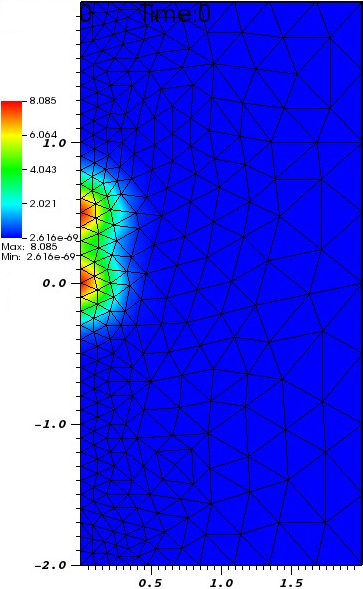
(a) $\tau=0$

(b) $\tau=\delta\tau$

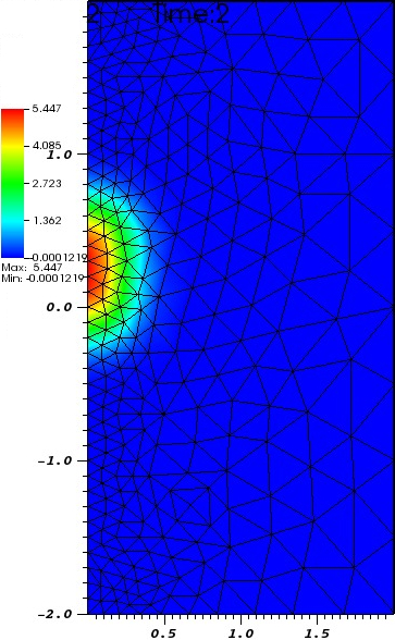
(c) $\tau=2\,\delta\tau$

(d) $\tau=4\,\delta\tau$

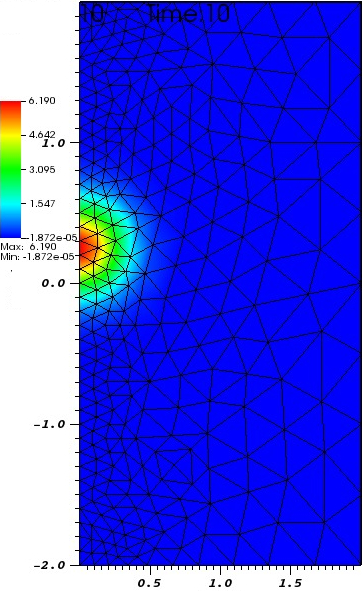
(e) $\tau=10\,\delta\tau$

(f) $\tau=20\,\delta\tau$

Figure 1: Time slices of an initially double Maxwellian distribution function relaxing towards an equilibrium state.

Table 1: Momentum conservation, measured with the innerproduct $\sum_{ij}\phi^{i}{\cal M}_{ij}F_{j}$ and $\phi=z$ for different nonlinear solver tolerances $\epsilon_{\textrm{tol}}$. The incorrect digits are highlighted with red color.

$\#\,\delta\tau$	$\epsilon_{\textrm{tol}}=$9.0E-01	$\epsilon_{\textrm{tol}}=$1.0E-06	$\epsilon_{\textrm{tol}}=$1.0E-14
0	3.97797664845241E-02	3.97797664845241E-02	3.97797664845248E-02
1	3.97791615978734E-02	3.97797664781777E-02	3.97797664845248e-02
2	3.97788912692161E-02	3.97797664743008E-02	3.97797664845247E-02
4	3.97786187222186E-02	3.97797664643968E-02	3.97797664845247E-02
10	3.97781761433900E-02	3.97797664423772E-02	3.97797664845247E-02
20	3.97775989653156E-02	3.97797663011934E-02	3.97797664845247E-02

Table 2: Energy conservation, measured with the innerproduct $\sum_{ij}\phi^{i}{\cal M}_{ij}F_{j}$ and $\phi=r^{2}+z^{2}$ for different nonlinear solver tolerances $\epsilon_{\textrm{tol}}$. The incorrect digits are highlighted with red color.

$\#\,\delta\tau$	$\epsilon_{\textrm{tol}}=$9.0E-01	$\epsilon_{\textrm{tol}}=$1.0E-06	$\epsilon_{\textrm{tol}}=$1.0E-14
0	3.17986788742740E-02	3.17986788742740E-02	3.17986788742740E-02
1	3.17606259814932E-02	3.17986790469298E-02	3.17986788742740E-02
2	3.17718385841557E-02	3.17986794847238E-02	3.17986788742741E-02
4	3.18140462853466E-02	3.17986808661484E-02	3.17986788742741E-02
10	3.18822521328414E-02	3.17986851426220E-02	3.17986788742741E-02
20	3.19077804661782E-02	3.17986927385047E-02	3.17986788742742E-02

V Summary

We have presented an algorithm for conservative discretization of the nonlinear Landau collision integral. We have provided both algebraic and numerical proof for achieving exact numerical conservation laws using either discontinuous Galerkin or standard finite-element method. Our method is not constrained by details of the discretization, admitting the use of structurized as well as unstructurized meshes. We have also argued that in the relativistic case, a polynomial basis of any order is not able to guarantee exact conservation of energy while density and momentum would be conserved even with linear basis functions. Future study will investigate the embedding of our discrete Landau operator to the Vlasov-Maxwell system using either the concept of Lagrange-d’Alembert principle or extended Lagrangians Kraus_Maj_2015 . Another future study will focus on performance demonstrations.

*

Appendix A Axially symmetric weak formulation

Using cylindrical coordinates $\bm{x}=(r,\theta,z)$, that relate to cartesian coordinates according to $(x,y,z)=(r\cos\theta,r\sin\theta,z)$, and assuming axially symmetric vector space $V$, i.e., $\partial f/\partial\theta=0$ and $\partial\phi/\partial\theta=0$, the weak formulation can be written

$$2\pi\int_{\Omega}drdz\;r\;\phi\;\partial_{\tau}f=\int_{\Omega}drdz\;r\;\partial_{\alpha}\phi\;\left(K^{\alpha}f-D^{\alpha\beta}\partial_{\beta}f\right)$$ (36)

where the friction and diffusion coefficients are

$$K^{\alpha} =\int_{\Omega}d\bar{r}d\bar{z}\;\bar{r}\;U^{\alpha\bar{\beta}}\partial_{\bar{\beta}}\bar{f}$$ (37)

$$D^{\alpha\beta} =\int_{\Omega}d\bar{r}d\bar{z}\;\bar{r}\;U^{\alpha\beta}\bar{f},$$ (38)

and the coefficients $U^{\alpha\beta}$ and $U^{\alpha\bar{\beta}}$ are defined

$$U^{\alpha\beta}=\int_{0}^{2\pi}\int_{0}^{2\pi}d\theta d\bar{\theta}\;\nabla x^{\alpha}\cdot\mathbf{U}\cdot\nabla x^{\beta}$$ (39)

$$U^{\alpha\bar{\beta}}=\int_{0}^{2\pi}\int_{0}^{2\pi}d\theta d\bar{\theta}\;\nabla x^{\alpha}\cdot\mathbf{U}\cdot\bar{\nabla}\bar{x}^{\beta}.$$ (40)

The expressions $\nabla x^{\alpha}$ are the contravariant basis vectors for the curvilinear coordinate system.

For the nonrelativistic case, the angular integrals of $\nabla x^{\alpha}\cdot\mathbf{U}\cdot\nabla x^{\beta}$ are easily computed. Defining a parameter

$$s(r,z,\bar{r},\bar{z})=\frac{2r\bar{r}}{r^{2}+\bar{r}^{2}+(z-\bar{z})^{2}},$$ (41)

the exact expressions are

$$U^{rr} =4\pi\left(\frac{s}{2r\bar{r}}\right)^{3/2}(\bar{r}^{2}{\cal I}_{1}+(z-\bar{z})^{2}{\cal I}_{2})$$ (42)

$$U^{rz} =4\pi\left(\frac{s}{2r\bar{r}}\right)^{3/2}(\bar{z}-z)(r{\cal I}_{2}-\bar{r}{\cal I}_{3})$$ (43)

$$U^{zr} =U^{rz}$$ (44)

$$U^{zz} =4\pi\left(\frac{s}{2r\bar{r}}\right)^{3/2}((r^{2}+\bar{r}^{2}){\cal I}_{2}-2r\bar{r}{\cal I}_{3})$$ (45)

$$U^{r\bar{r}} =4\pi\left(\frac{s}{2r\bar{r}}\right)^{3/2}((z-\bar{z})^{2}{\cal I}_{3}+r\bar{r}{\cal I}_{1})$$ (46)

$$U^{r\bar{z}} =U^{rz}$$ (47)

$$U^{z\bar{r}} =4\pi\left(\frac{s}{2r\bar{r}}\right)^{3/2}(\bar{z}-z)(r{\cal I}_{3}-\bar{r}{\cal I}_{2})$$ (48)

$$U^{z\bar{z}} =U^{zz}$$ (49)

where the integrals ${\cal I}(s)$ are defined

$${\cal I}_{1}(s) =\int_{-1}^{1}(1-x^{2})^{1/2}(1-sx)^{-3/2}dx$$ (50)

$${\cal I}_{2}(s) =\int_{-1}^{1}(1-x^{2})^{-1/2}(1-sx)^{-3/2}dx$$ (51)

$${\cal I}_{3}(s) =\int_{-1}^{1}x(1-x^{2})^{-1/2}(1-sx)^{-3/2}dx$$ (52)

and can be expressed in terms of the complete elliptic integrals $E[s]$ and $K[s]$ according to

$${\cal I}_{1}(s) =\frac{4}{s^{2}\sqrt{1+s}}\left(K\left[\frac{2s}{1+s}\right]-(1+s)E\left[\frac{2s}{1+s}\right]\right),$$ (53)

$${\cal I}_{2}(s) =\frac{2}{(1-s)\sqrt{1+s}}E\left[\frac{2s}{1+s}\right],$$ (54)

$${\cal I}_{3}(s) =\frac{2}{(1-s)s\sqrt{1+s}}\left(E\left[\frac{2s}{1+s}\right]-(1-s)K\left[\frac{2s}{1+s}\right]\right)$$ (55)

A similar computation of the axisymmetric coefficients was demonstrated in Yoon_et_al_2014 .

References

- [1] Hong Qin and Xiaoyin Guan. Variational symplectic integrator for long-time simulations of the guiding-center motion of charged particles in general magnetic fields. Phys. Rev. Lett., 100:035006, Jan 2008.
- [2] J. Squire, H. Qin, and W. M. Tang. Geometric integration of the Vlasov-Maxwell system with a variational particle-in-cell scheme. Physics of Plasmas, 19(8):084501, 2012.
- [3] Michael Kraus. Variational Integrators in Plasma Physics. PhD thesis, Technische Universität München, 2013.
- [4] C Leland Ellison, J M Finn, H Qin, and W M Tang. Development of variational guiding center algorithms for parallel calculations in experimental magnetic equilibria. Plasma Physics and Controlled Fusion, 57(5):054007, 2015.
- [5] Hong Qin, Jian Liu, Jianyuan Xiao, Ruili Zhang, Yang He, Yulei Wang, Yajuan Sun, Joshua W. Burby, Leland Ellison, and Yao Zhou. Canonical symplectic particle-in-cell method for long-term large-scale simulations of the vlasov-maxwell equations. Nuclear Fusion, 56(1):014001, 2016.
- [6] Yang He, Yajuan Sun, Hong Qin, and Jian Liu. Hamiltonian particle-in-cell methods for Vlasov-Maxwell equations. Physics of Plasmas, 23(9):092108, 2016.
- [7] Yao Zhou, Hong Qin, J. W. Burby, and A. Bhattacharjee. Variational integration for ideal magnetohydrodynamics with built-in advection equations. Physics of Plasmas, 21(10):102109, 2014.
- [8] L.D. Landau. The kinetic equation in the case of Coulomb interaction (translated from German). Zh. Eksper. i Teoret. Fiz., 7:203–209, 1937.
- [9] P. J. Morrison. A paradigm for joined Hamiltonian and dissipative systems. Physica D Nonlinear Phenomena, 18:410–419, January 1986.
- [10] Marshall N. Rosenbluth, William M. MacDonald, and David L. Judd. Fokker-planck equation for an inverse-square force. Phys. Rev., 107:1–6, Jul 1957.
- [11] W.T. Taitano, L. Chacón, A.N. Simakov, and K. Molvig. A mass, momentum, and energy conserving, fully implicit, scalable algorithm for the multi-dimensional, multi-species Rosenbluth–Fokker–Planck equation. Journal of Computational Physics, 297:357–380, 2015.
- [12] E. S. Yoon and C. S. Chang. A Fokker-Planck-Landau collision equation solver on two-dimensional velocity grid and its application to particle-in-cell simulation. Physics of Plasmas, 21(3):032503, 2014.
- [13] Robert Hager, E.S. Yoon, S. Ku, E.F. D’Azevedo, P.H. Worley, and C.S. Chang. A fully non-linear multi-species Fokker–Planck–Landau collision operator for simulation of fusion plasma. Journal of Computational Physics, 315:644–660, 2016.
- [14] J. W. Burby, A. J. Brizard, and H. Qin. Energetically consistent collisional gyrokinetics. Physics of Plasmas, 22(10):100707, October 2015.
- [15] S. T. Beliaev and G. I. Budker. The Relativistic Kinetic Equation. Soviet Physics Doklady, 1:218, Oct 1956.
- [16] C. Geuzaine and J.-F. Remacle. Gmsh: a three-dimensional finite element mesh generator with built-in pre- and post-processing facilities. International Journal for Numerical Methods in Engineering, 79:1309–1331, 2009.
- [17] Satish Balay, Shrirang Abhyankar, Mark F. Adams, Jed Brown, Peter Brune, Kris Buschelman, Lisandro Dalcin, Victor Eijkhout, William D. Gropp, Dinesh Kaushik, Matthew G. Knepley, Lois Curfman McInnes, Karl Rupp, Barry F. Smith, Stefano Zampini, Hong Zhang, and Hong Zhang. PETSc Web page. http://www.mcs.anl.gov/petsc, 2016.
- [18] Satish Balay, Shrirang Abhyankar, Mark F. Adams, Jed Brown, Peter Brune, Kris Buschelman, Lisandro Dalcin, Victor Eijkhout, William D. Gropp, Dinesh Kaushik, Matthew G. Knepley, Lois Curfman McInnes, Karl Rupp, Barry F. Smith, Stefano Zampini, Hong Zhang, and Hong Zhang. PETSc users manual. Technical Report ANL-95/11 - Revision 3.7, Argonne National Laboratory, 2016.
- [19] Michael Kraus and Omar Maj. Variational integrators for nonvariational partial differential equations. Physica D: Nonlinear Phenomena, 310:37–71, 2015.