Modeling and Measuring Impact of Adaptive and Cooperative Adaptive Cruise Control on Throughput of Signalized Intersections

Abstract

To properly assess the impact of (cooperative) adaptive cruise control ACC (CACC), one has to model vehicle dynamics. First of all, one has to choose the car following model, as it determines the vehicle flow as vehicles accelerate from standstill or decelerate because of the obstacle ahead. The other factor significantly affecting the intersection throughput is the maximal vehicle acceleration rate.

In this paper, we analyze three car following behaviors: Gipps model, Improved Intelligent Driver Model (IIDM) and Helly model. Gipps model exhibits rather aggressive acceleration behavior. If used for the intersection throughput estimation, this model would lead to overly optimistic results. Helly model is convenient to analyze due to its linear nature, but its deceleration behavior in the presence of obstacles ahead is unrealistically abrupt. Showing the most realistic acceleration and deceleration behavior of the three models, IIDM is suited for ACC/CACC impact evaluation better than the other two.

We discuss the influence of the maximal vehicle acceleration rate and presence of different portions of ACC/CACC vehicles on intersection throughput in the context of the three car following models. The analysis is done for two cases: (1) free road downstream of the intersection; and (2) red light at some distance downstream of the intersection.

Finally, we introduce the platoon model and evaluate ACC and CACC with platooning in terms of travel time using SUMO simulation of a traffic network with 7 intersections in North Bethesda, MD.

Keywords: signalized intersections, adaptive cruise control (ACC), cooperative adaptive cruise control (CACC), car following models, Helly Model, Gipps Model, Improved Intelligent Driver Model

1 Introduction and Background

Urban transportation is heading towards a crisis. According to the 2015 Urban Mobility Scorecard [39], travel delays due to traffic congestion caused drivers to waste more than 3 billion gallons of fuel and kept travelers stuck in their cars for nearly 7 billion extra hours — 42 hours per rush-hour commuter. The total nationwide price tag: $160 billion, or $960 per commuter. Almost two thirds of congestion in large cities (and more than 80% in smaller urban areas) occur on city streets.

Intersections are the major bottlenecks of the city road networks because an intersection’s capacity is only a fraction of the vehicle flows that the streets connecting to the intersection can carry. Traditional way of controlling traffic on city streets is through adjusting signal timing. There is a substantial body of work addressing signal optimization. Tuning of cycle length is discussed in [24, 6]. Route prioritization through split adjustment is described in [40]. The max-pressure local feedback control policy that gives priority to movements with larger queues is also working with splits [47]. Bandwidth maximization through offsets problem was solved in different variations in [31, 29, 14, 34, 35, 15]. This work was analyzed and a new formulation relying on the concepts of relative offset and vehicle arrival functions together with an efficient computation technique was proposed in [19]. These results were extended in [10] to optimize energy consumption via signal offsets control and variable speed limits. A review of adaptive signal systems is given in [3] and Traffic-responsive Urban Control (TUC) strategy is described in [11]. There is also an active research on improving intersection performance by fully shifting the traffic control to vehicles [4, 5]. These approaches, however, are based on the assumption that all vehicles can communicate with each other, which at present is unrealistic.

It is argued in [27] that as a combination of efficient signal control, proper utilization of new vehicle technologies, multimodal transportation; and parking management. This paper presents an empirical study of how the existing technologies, such as adaptive cruise control (ACC), and the emerging technologies, such as cooperative adaptive cruise control (CACC) [30], can mitigate the congestion problem on city streets by increasing the throughput of intersections, as vehicles equipped with ACC/CACC can travel closer to each other and even form platoons. Platoons were shown to improve freeway throughput [46], and recently in [12]. In [28] the authors suggest that the saturation flow rates, and hence intersection capacity, can be [at least] doubled by platooning. However, that argument rests on the results of Point Queue modeling of signalized arterials, which do not take into account vehicle dynamics and car following behavior.

To better assess the impact of ACC and CACC vehicles on intersection throughput, one has to model car following behavior. The choice of the car following models largely determines the findings of of the ACC/CACC impact study. There is a variety of car following models. The list starts with the Reuschel [37] and Pipes [36] models, in which the speed changes instantaneously as a function of the distance to the leading vehicle. Another class of models, generally referred to as Gazis-Herman-Rothery (GHR) [9, 16], is where the acceleration depends on speed difference and the distance gap according to the power law and not influenced by the driver’s own speed. These models are incomplete in the following sense: they can describe either free traffic or approach to standing obstacle, but not both. On the contrary, complete models describe all situations, including acceleration and cruising in free traffic, following other vehicles in stationary and non-stationary situations, and approaching slow or standing vehicles, and red lights [43] (Chapter 10).

The class of models, where the acceleration depends on speed difference with car in front and on the difference between the actual and the desired gap linearly, is attributed to Helly [20]. Helly model is complete, and its linear nature makes it easy to understand and analyze. It was extensively studied, built upon and used for ACC/CACC modeling [41, 18, 45, 21, 44].

Another example of a complete model is the Optimal Velocity Model (OVM) [7]. In OVM, acceleration depends only on the distance (but not on the speed difference) to the car in front: this distance determines the optimal speed, which the vehicle tries to hold. OVM is not always collision-free. Full Velocity Difference Model (FVDM) [22] extends OVM by adding the linear dependence on the speed difference with the car in front to the acceleration equation. Generally considered more realistic than OVM, in terms of acceleration values and the shock waves that it produces, FVDM suffers from the defect that it is not complete in the sense defined above. The reason is that the speed difference term does not depend on the gap between the vehicle and the car in front. Consequently, a slow vehicle triggers a significant deceleration of its follower even if it is miles away. Newell car following model [32, 33], describes car-following behaviour based on the analysis of time-space trajectory, assuming that the time-space trajectory for two adjacent vehicles is essentially the same, except for the shift in time and space. For gaps smaller than desired and triangular fundamental diagram, the Newell model behaves the same OVM.

All the above mentioned models are heuristic — they attempt to describe vehicle flow based on observations and common sense. Gipps car following model [17] and the Intelligent Driver Model (IDM) [42] are similar to complete heuristic models in that they too are defined by their acceleration equations. In addition to that, they adhere the following principles:

1. the model is complete in the sense of the definition above;

2. the equilibrium gap to the car in front is no less than the safe distance computed as a sum of the minimal gap and the distance the car can travel during the period called reaction time;

3. deceleration increases and decreases smoothly under normal driving conditions, but can exceed “comfortable” level when the car in front is too close and too slow — to avoid collision;

4. transitions between different driving modes are smooth;

5. each model parameter describes only one aspect of driving behavior;

6. acceleration is strictly decreasing function of the speed;

7. acceleration is an increasing function of the gap between the vehicle and the car in front;

8. acceleration is an increasing function of the speed of the car in front;

9. minimal gap to the car in front is maintained even during standstill, but there is no backward movement if the gap is smaller than the minimal (e.g. due to initial conditions).

Gipps model is widely used and is implemented in the Aimsun microsimulator. Krauss car following model [26] is a stochastic variation of Gipps model, where an auto-correlated noise is added to the vehicle speed. Krauss-Gipps model is implemented in the SUMO microsimulator [25]. IDM is considered to have more realistic acceleration profile than that of Gipps model. It is widely investigated for the purpose of ACC/CACC implementation [23, 38, 48, 30]. Due to the continuous transition between free flow and congested traffic, the gap between vehicles grows infinitely large as the speed approaches the equilibrium value. The other effect of this continuous transition is that the gap size between the vehicle and the car in front smaller than desired leads to unrealistically high deceleration values. This produces unacceptable vehicle behavior in platoons. Therefore, the acceleration function was modified to retain the spirit of IDM but to eliminate its shortcomings. The resulting model is called Improved IDM (IIDM) [43] (Chapter 11). Gipps model and IIDM are sometimes called first principle models, referring to the four principles stated above.

Finally, there is a category of car following models referred to as behavioral. These are Wiedemann [49, 50] and Fritzsche [13] models, implemented in PTV Vissim and Paramics simulators respectively. These two models are essentially hybrid systems, where guards between different modes of vehicle dynamics are thresholds for the speed difference and the distance to the car in front. Adjusting those guards changes driver behavior in the range from overly cautious to aggressive and from slow reactive to fast. In the Wiedemann and Fritzsche models, transitions between different driving modes are not necessarily smooth, as acceleration changes in a series of discrete transitions, which violates rule 4 of the first principles listed above. Designed to model human behavior and requiring complex tuning of the multitude of parameters, these models are generally not used for ACC/CACC.

In this paper we analyze three models — Gipps, IIDM and Helly — and assess the impact of ACC and CACC vehicles on the intersection throughput in the context of these models. The rest of the paper is organized as follows. In Section 2, we review Gipps model, IIDM and Helly model and analyze their properties in the context of signalized arterials. In Section 3, we derive the macroscopic models corresponding the three car following models in question. In Section 4, we investigate the impact of ACC- and CACC-enabled traffic on intersection throughput. In Section 5 we introduce the platoon model, and evaluate it in the simulation of North Bethesda road network, a case study presented in Section 6. Section 7 concludes the paper.

2 Analysis of Car Following Models

We start by introducing the notation that will be used in the car following model discussion. It is summarized in Table 1 together with the default parameter values that we will use in our experiments, unless stated otherwise.

Symbol	Description	Default value
$l$	Vehicle length.	$l=5$ m.
$t$, $\Delta t$	Time and the model time step.	$\Delta t=0.05$ s.
$x(t)$	Vehicle position.
$x_{l}(t)$	Position of the vehicle in front, the leader.
$v_{\max}$	Maximal admissible speed for the vehicle.	$v_{\max}=20$ m/s.
$v(t)$	Vehicle speed.
$v_{l}(t)$	Speed of the leader.
$a(t)$	Vehicle acceleration.
$a_{\max}$	Maximal vehicle acceleration.	$a_{\max}=1.5\mbox{ m/s}^{2}$.
$b$	Desired vehicle deceleration.	$b=2\mbox{ m/s}^{2}$.
$g(t)$	Gap: distance from the front of the vehicle to the tail of the leader, $g(t)=x_{l}(t)-x(t)-l$.
$g_{\min}$	Minimal gap that is allowed between the vehicle and the leader.	$g_{\min}=4$ m.
$g_{d}(t)$	Desired gap between the vehicle and the leader.
$\tau$	Reaction time to decelerate for the vehicle to avoid collision with the leader.	$\tau=2.05$ s.
$\theta(t)$	Headway: $\theta(t)=\frac{x_{l}(t)-x(t)}{v(t)}$.
$f(t)$	Vehicle flow: $f(t)=\frac{1}{\theta(t)}$.

Table 1: Notation for car following models.

The state update equations for a car following model are:

$$v(t+\Delta t) = v(t)+a(t)\Delta t;$$ (2.1)

$$x(t+\Delta t) = x(t)+\frac{v(t)+v(t+\Delta t)}{2}\Delta t=x(t)+v(t)\Delta t+\frac{a(t)\Delta t^{2}}{2},$$ (2.2)

where acceleration $a(t)$ depends on the car following model — Gipps, IIDM and Helly — whose descriptions follow.

• Gipps model:

  $$a(t)=\min\left\{a_{\max},\frac{v_{\max}-v(t)}{\Delta t},\frac{1}{\Delta t}\left(-v(t)-b\tau+\sqrt{(b\tau)^{2}+(v_{l}(t))^{2}+2b\left(g(t)-g_{\min}\right)}\right)\right\}.$$ (2.3)

• IIDM:

  $$a(t)=\left\{\begin{array}[]{ll}a_{\max}\left(1-\left(\frac{g_{d}(t)}{g(t)}\right)^{\delta_{1}}\right),&\mbox{ if }\frac{g_{d}(t)}{g(t)}>1;\\ a^{\ast}(t)\left(1-\left(\frac{g_{d}(t)}{g(t)}\right)^{\delta_{1}a_{\max}/a^{\ast}(t)}\right),&\mbox{ otherwise,}\end{array}\right.$$ (2.4)

  where

  $$a^{\ast}(t) = a_{\max}\left(1-\left(\frac{v(t)}{v_{\max}}\right)^{\delta_{2}}\right),$$ (2.5)

  $$g_{d}(t) = g_{\min}+\max\left\{0,v(t)\tau+\frac{v(t)(v(t)-v_{l}(t))}{2\sqrt{a_{\max}b}}\right\},$$ (2.6)

  and $\delta_{1},\delta_{2}$ are some fixed positive parameters.

• Helly model:

  $$a(t)=\min\left\{a_{\max},\frac{v_{\max}-v(t)}{\Delta t},\alpha_{1}\left(v_{l}(t)-v(t)\right)+\alpha_{2}\left(g(t)-g_{\min}-v(t)\tau\right)\right\},$$ (2.7)

  where $\alpha_{1}$ and $\alpha_{2}$ are some positive fixed parameters.

In all three models, the equilibrium speed ($a(t)=0$) is achieved with $v(t)=v_{l}(t)=v_{\max}$ and $g(t)=g_{\min}+v(t)\tau$. In this case, equilibrium headway is:

$$\theta_{e}=\tau+\frac{g_{\min}+l}{v_{\max}}.$$ (2.8)

Assuming default values from Table 1, the length of the car $l=5$ m, the speed limit $v_{\max}=20$ m/s, the minimal gap $g_{\min}=4$ m and the reaction time $\tau=2.05$ s, from (2.8) we get $\theta_{e}=2.5$ s, which translates to $f_{e}=1/\theta_{e}=0.4$ vehicles per second, 24 vehicles per minute, or 1440 vehicles per hour.

Now let us compare the behavior of these car following models in three experiments with intersections. In these experiments we will be using the parameter values from Table 1, and specific IIDM and the Helly model parameters given in Table 2.

$\delta_{1}=8$

$\delta_{2}=4$

$\alpha_{1}=0.5$

$\alpha_{2}=0.25$

Table 2: Parameter values used for IIDM and the Helly model.

Experiment with a free road ahead.
Consider a setup presented in Figure 1.

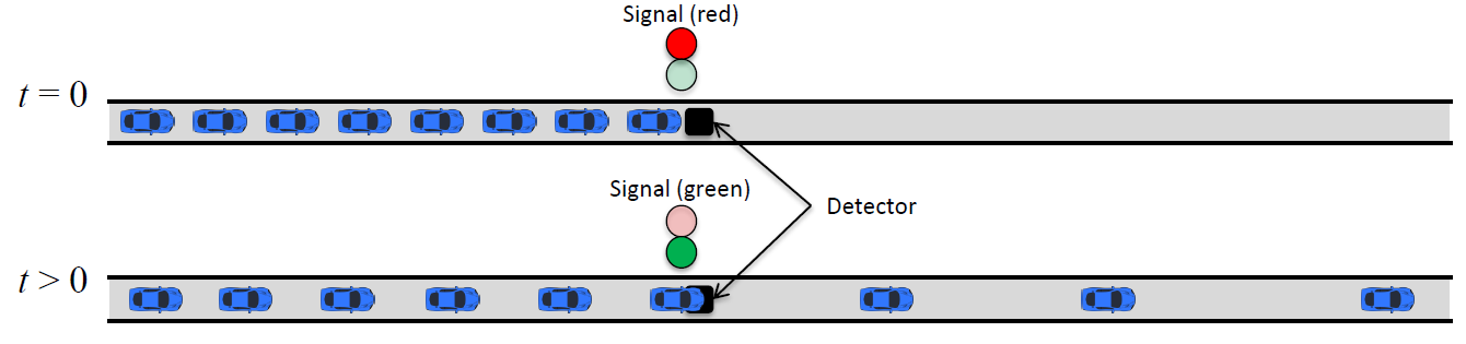
Figure 1: Signal turns green at time $t=0$, and vehicles start moving. The first vehicle has free road ahead.

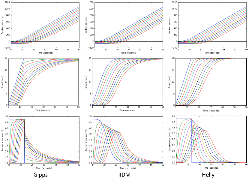
Figure 2: Experiment with a free road ahead: comparison of vehicle trajectories, speeds and accelerations between the three car following models.

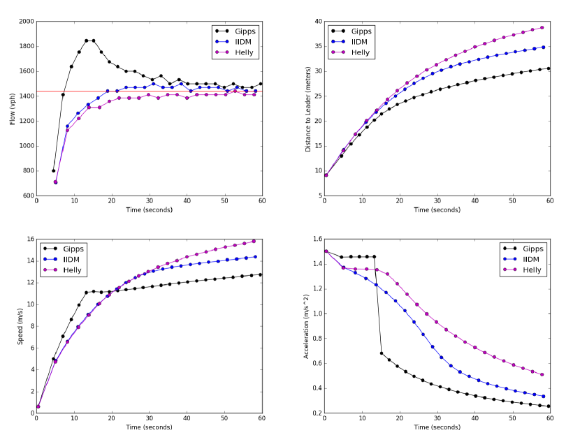
Figure 3: Experiment with a free road ahead: comparison of point measurements of flow, distance to leader, speed and acceleration at the detector location between the three car following models.

The initial condition at time $t=0$ is that infinite number of vehicles are standing in the queue with the minimal gap between them. The light turns green, and vehicles are released.

Figure 2 shows trajectories, speeds and accelerations of the first ten vehicles from the queue computed by the three car following models. The signal is located at position 0 indicated by the horizontal black line in the top three trajectory plots. The first vehicle is governed by the car following model just as everyone else, but its leader is infinitely far. From the acceleration and speed plots one can see that in the Gipps and the Helly models the first vehicle accelerates with maximal acceleration $a_{\max}$ until reaching the maximal speed, at which point the acceleration instantaneously drops to 0. In the IIDM, the first vehicle accelerates with $a^{\ast}(t)$ from equation (2.5), approaching the maximal speed asymptotically.

The most important for the intersection throughput assessment, however, is the traffic behavior at the stop bar — at the detector location indicated in Figure 1. Figure 3 presents the point measurments obtained from this detector location, with each dot corresponding to a vehicle passing the detector. Flow (top left) is computed for a vehicle passing the detector based on the time passed after the previously detected vehicle, taken as a headway $\theta(t)$, which is then inverted ($f(t)=1/\theta(t)$) and converted to vehicles per hour (vph). The red horizontal line corresponds to the equilibrium flow, in our case — 1440 vph, when vehicles move at maximal speed. Gap (top right) between vehicles as well as speed (bottom left) are monotonically increasing, while acceleration (bottom right) is monotonically decreasing.

As is evident from plots in Figure 3, Gipps model produces rather aggressive car following pattern to the point that it manages to push through the intersection 26 vehicles per minute, two more than would pass through the intersecton in an equilibrium flow (24 vehicles per minute), while IIDM and Helly model push through 23 and 22 vehicles per minute respectively — see the middle row (free road ahead) of Table 3. What is interesting about this observation, is that with the Gipps model one could argue that a signal would increase the road throughput by creating pulses in the vehicle flow, as the one in Figure 3 (top left). Moreover, the smaller the signal cycle, the bigger will be the throughput increase. This is counterintuitive and, likely, unrealistic. IIDM and Helly model can be tuned to behave more agressively by increasing their parameters $\delta_{1},\delta_{2}$ in IIDM and $\alpha_{1},\alpha_{2}$ in Helly. Neither of these two models, however, can reach the throughput result of Gipps.

Experiment with a red light downstream.
Let us modify the experiment setup by introducing the second intersection downstream of the first one, where vehicles have to stop at the red light — Figure 4 depicts the modified configuration.

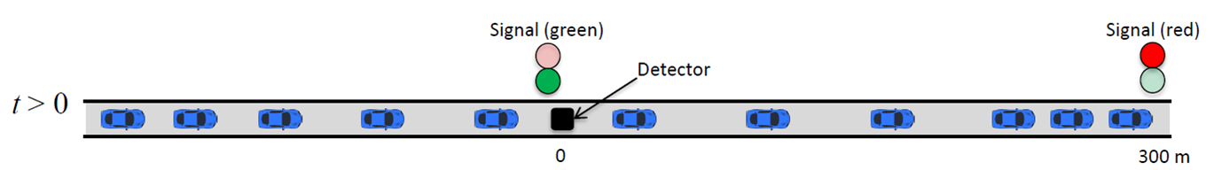
Figure 4: Signal turns green at time $t=0$, and vehicles start moving. The first vehicle encounters red light in the next intersection 300 meters downstream.

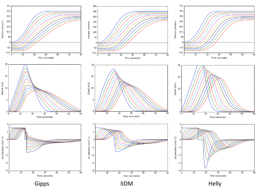
Figure 5: Experiment with a red light ahead: comparison of vehicle trajectories, speeds and accelerations between the three car following models.

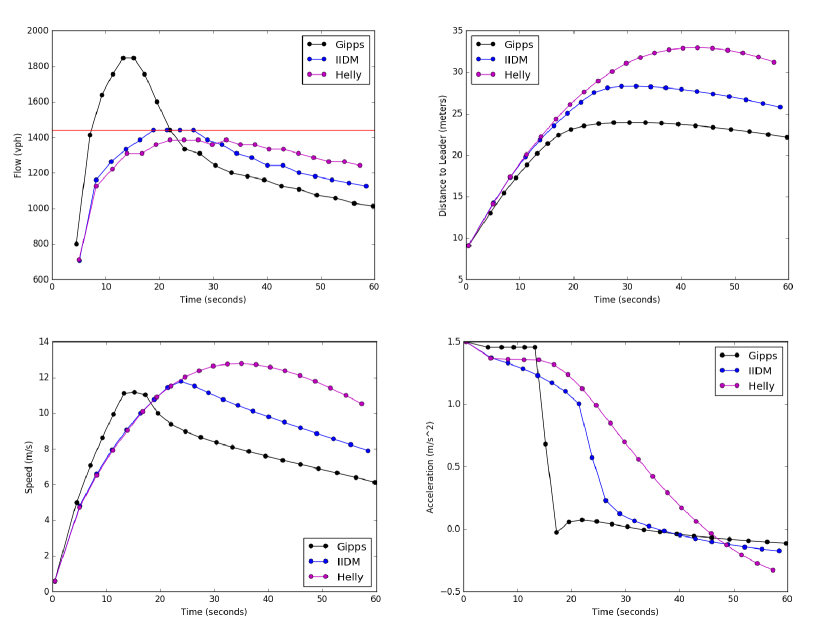
Figure 6: Experiment with a red light ahead: comparison of point measurements of flow, distance to leader, speed and acceleration at the detector location between the three car following models.

In this experiment, the second intersection is 300 meters away from the first one. This distance is enough to hold 33 vehicles in the queue (see Table 1 for default values of the car length $l$ and the minimal gap $g_{\min}$), which is more than the most aggressive, Gipps, car following model can send in one minute.

It is important to note that if instead of any car following model we were using a Point Queue model with limited or unlimited queues, such as in [28], we would be able to send as many vehicles through the first intersection, as our saturation flow setting would allow. In the case of our example, if we set the saturation flow to 24 vehicles per minute (equal to our equilibrium flow), after 1 minute of green light in the first intersection, 24 vehicles would be transferred from the first queue to the next, in front of the second intersection. The car following model, on the other hand, exhibits the braking effect that propagates back and reduces the vehicle flow though the first intersection. In the experiment with the red light downstream we study the impact of this braking effect on the throughput of the first intersection.

Figure 5 shows trajectories, speeds and accelerations of the first ten vehicles from the queue computed by the three car following models. The first signal is at position 0 indicated by the horizontal black line in the top three trajectory plots, and the second signal is at position $x_{s}=300$. To make the first vehicle stop at $x_{s}$, we place a “blocking vehicle” in front at position

$$x_{b}=x_{s}+g_{\min}+l=300+4+5=309,$$

with velocity $v_{b}=0$. Governed by the car following model, the first vehicle stops at position $x_{s}$ to maintain the minimal gap with this virtual “blocking vehicle”. In our case, the first vehicle in the Gipps and the Helly models reaches the maximal speed before starting to brake. Moreover, in the Helly model the first vehicle continues with the maximal longer than in Gipps, allowing the second vehicle to almost reach the maximal speed, which then leads to prohibitively sharp deceleration jump. In contrast, in IIDM the first vehicle starts to brake earlier than in Gipps and Helly models, even before reaching the maximal speed, resulting in smooth speed curves.

Point measurements taken at the detector location, shown in Figure 4, and presented in Figure 6, indicate the reduction in flow through the first intersection as the result of the braking propagation. Gipps, IIDM and Helly models manage to send 22, 21 and 21 vehicles per minute respectively through the first intersection — see the middle row (red light ahead) of Table 3. As before, the red horizontal line in the top left plot corresponds to the equilibrium flow, in our case — 1440 vph, when vehicles move at maximal speed. These plots also indicate the reactiveness of the studied car following models: how fast the cars upstream react to the behavior of the first vehicle. Given the IIDM and Helly model parameter values from Table 2, Gipps model has the shortest reaction time, followed by IIDM and then, by Helly model.

Experiment with different accelerattion levels.
Now, let us explore how throughput of the first intersection in our two previous experiments depends on the maximal acceleration $a_{\max}$. We repeat both experiments, with the free road and with the red light ahead, for three different values of $a_{\max}$: $0.8$, $1.5$ (our default) and $2.5\mbox{ m/s}^{2}$.

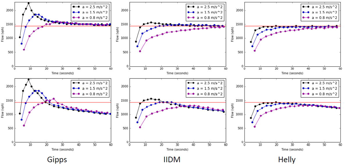
Figure 7: Comparing flows for different values of $a_{\max}$ for two experiments — with the free road (top), and with the red light ahead (bottom).

Value of $a_{\max}$	Type of experiment	Gipps model	IIDM	Helly model
$0.8\mbox{ m/s}^{2}$	free road ahead	23	20	20
	red light ahead	20	19	20
$1.5\mbox{ m/s}^{2}$	free road ahead	26	23	22
	red light ahead	22	21	21
$2.5\mbox{ m/s}^{2}$	free road ahead	27	24	23
	red light ahead	22	22	22

Table 3: Summary of three experiments — intersection throughput in vehicles per minute. Values equal to or exceeding the equilibrium flow, 24 vehicles per minute, are given in bold.

Figure 7 presents the point measurements obtained from the detector location for the cases of free road (top) and red light downstream (bottom). Table 3 summarizes the throughput results for all the model-accelertion-experiment combinations.

The main findings of this experiment are:

• with low $a_{\max}$ and braking effect, Helly model produces larger throughput than IIDM, whereas generally the opposite is true;

• with low $a_{\max}$, IIDM and Helly model behave similarly;

• with high $a_{\max}$ and braking effect, the all three models produce the same throughput;

• braking effect reduces the impact of $a_{\max}$ parameter on throughput.

To perform a spacial analysis of the traffic flow shock wave propagation for different values of $a_{\max}$, we have to translate the car following behavior into a macroscopic model, which we do next.

3 Micro-to-Macro Translation

Macroscopic models describe traffic in terms of density, and speed. The road is divided into $1,\dots,N$ links, and the state of the system at time $t$ is given by the density-speed pair $\{\rho_{i}(t),V_{i}(t)\}_{1}^{N}$. Table 4 contains the notation used in macro-modeling.

Symbol	Description	Default value
$\Delta x_{i}$	Length of link $i$.	$\Delta x_{i}=5$ m.
$t$, $\Delta t$	Time and the model time step (same as in the car following model).	$\Delta t=0.05$ s.
$\rho_{i}(t)$	Vehicle density in link $i$.
$\rho_{J}$	Maximal admissible (jam) density.	$\rho_{J}=1/9$ veh. per meter.
$V_{i}(t)$	Average traffic speed link $i$.
$v_{\max}$	Maximal admissible traffic speed (same as in the car following model).	$v_{\max}=20$ m/s.
$f_{i}(t)$	Vehicle flow out of link $i$.
$f_{0}(t)$	Vehicle flow entering link $1$.

Table 4: Macro-modeling notation.

Vehicle density $\rho_{i}t)$ is computed from the gap between vehicles and the vehicle length:

$$\rho_{i}(t)=\frac{1}{g_{i}(t)+l},$$ (3.1)

where notation $g_{i}(t)$ defines average gap between vehicles that are in link $i$ at time $t$. Obviously, $\rho_{i}(t)\leq\rho_{J}=\frac{1}{g_{\min}+l}$.

Every time step, density values in each link are updated according to the conservation law:

$$\rho(t+\Delta t)=\rho_{i}(t)+\frac{\Delta t}{\Delta x_{i}}\left(f_{i-1}(t)-f_{i}(t)\right),\;\;\;i=1,\dots,N,$$ (3.2)

where $f_{i}(t)=\rho_{i}(t)V_{i}(t)$, and the entering flow $f_{0}(t)$ is given.

The speed equation is derived from vehicle speed. For points $(t,x)$ on the trajectory of a vehicle, we can write:

$$v(t)=V(t,x).$$

The change in position during one time step $\Delta t$ can be expressed by the first order Taylor expansion around $(t,x)$:

$$v(t+\Delta t) = V(t+\Delta t,x+v(t)\Delta t)$$

$$= V(t,x)+\frac{\partial V(t,x)}{\partial t}\Delta t+\frac{\partial V(t,x)}{\partial x}v(t)\Delta t$$

$$= V(t,x)+\left(\frac{\partial V}{\partial t}+V(t,x)\frac{\partial V}{\partial x}\right)\Delta t.$$

At the same time, from the car following model we have:

$$v(t+\Delta t)=v(t)+a(t)\Delta t.$$

Thus, we get:

$$V(t,x)+\left(\frac{\partial V}{\partial t}+V(t,x)\frac{\partial V}{\partial x}\right)\Delta t=V(t,x)+a(t)\Delta t,$$

which, after cancelling $V(t,x)$ and dividing both sides of the equation by $\Delta t$, yields:

$$\frac{\partial V}{\partial t}+V(t,x)\frac{\partial V}{\partial x}=a(t).$$

Discretizing this equation in time and space, we can write:

$$\frac{V_{i}(t+\Delta)-V_{i}(t)}{\Delta t}+V_{i}(t)\frac{V_{i}(t)-V_{i-1}(t)}{\Delta x_{i}}=a_{i}(t),\;\;\;i=1,\dots,N,$$

and $V_{0}(t)=V_{1}(t)$.

Thus, we obtain the speed equation:

$$V_{i}(t+\Delta t)=V(t)+\left(a_{i}(t)-V_{i}(t)\frac{V_{i}(t)-V_{i-1}(t)}{\Delta x_{i}}\right)\Delta t.$$ (3.3)

Here $a_{i}(t)$ is defined by the car following model.

• For Gipps model, following (2.3), we have:

  $$a_{i}(t)=\min\left\{a_{\max},\frac{v_{\max}-V_{i}(t)}{\Delta t},\frac{-V_{i}(t)-b\tau+\sqrt{(b\tau)^{2}+(V_{i+1}(t))^{2}+2b\left(\frac{1}{\rho_{i}(t)}-\frac{1}{\rho_{J}}\right)}}{\Delta t}\right\},$$ (3.4)

  $i=1,\dots,N$; $V_{N+1}=v_{\max}$.

• For IIDM, following (2.4), we have:

  $$a_{i}(t)=\left\{\begin{array}[]{ll}a_{\max}\left(1-\frac{g_{d,i}(t)}{g_{i}(t)}\right),&\mbox{ if }\frac{g_{d,i}(t)}{g_{i}(t)}\geq 1,\\ a_{i}^{\ast}(t)\left(1-\left(\frac{g_{d,i}(t)}{g_{i}(t)}\right)^{\delta_{1}a_{\max}/a_{i}^{\ast}(t)}\right),&\mbox{ otherwise},\end{array}\right.$$ (3.5)

  where

  $$a_{i}^{\ast}(t)=a_{\max}\left(1-\left(\frac{V_{i}(t)}{v_{\max}}\right)^{\delta_{2}}\right),$$ (3.6)

  while the actual gap, $g_{i}(t)$, and the desired gap, $g_{d,i}(t)$, can be expressed through density:

  $$g_{i}(t)=\frac{1}{\rho_{i}(t)}-l,\;\;\;i=1,\dots,N,$$ (3.7)

  and

  $$g_{d,i}(t)=\frac{1}{\rho_{J}}-l+\max\left\{0,V_{i}(t)\tau+\frac{V_{i}(t)(V_{i}(t)-V_{i+1}(t))}{2\sqrt{a_{\max}b}}\right\},\;\;i=1,\dots,N;\;\;V_{N+1}=v_{\max}.$$ (3.8)

• For Helly model, following (2.7), we have:

  $$a_{i}(t)=\min\left\{a_{\max},\frac{v_{\max}-V_{i}(t)}{\Delta t},\alpha_{1}\left(V_{i+1}(t)-V_{i}(t)\right)+\alpha_{2}\left(\frac{1}{\rho_{i}(t)}-\frac{1}{\rho_{J}}-V_{i}(t)\tau\right)\right\},$$ (3.9)

  $i=1,\dots,N$; $V_{N+1}=v_{\max}$.

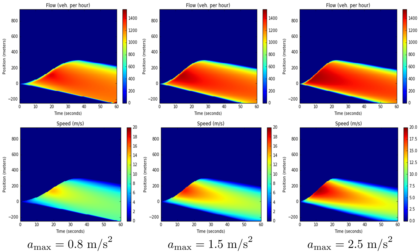
Figure 8: Flow (top) and speed (bottom) contours generated by the IIDM-induced macroscopic model in the experiment with the red light downstream for $a_{\max}=0.8$, $1.5$ and $2.5\mbox{ m/s}^{2}$.

As an example, we reproduced the experiment with the red light ahead and the red light at the second intersection in the macroscopic environment. The road is split into 240 links, each with length $l=5$ meters. The first signal is located at link 50. The initial condition is:

$$\rho_{i}(0)=\rho_{J}=\frac{1}{g_{\min}+l}=\frac{1}{4+5}=1/9,\;\;\;1=1,\dots,49;$$

$$\rho_{i}(0)=0,\;\;\;i=50,\dots,N=240;$$

$$V_{i}(0)=0,\;\;\;i=1,\dots,N=240.$$

The second signal with the red light is in link 110 (300 meters downstream of the first one), which translates into condition:

$$f_{110}(\cdot)=0.$$

Figure 8 presents the flow and speed contours, produced by the simulation of 60 seconds of the IIDM-induced macroscopic model for $a_{\max}=0.8,1.5$ and $2.5\mbox{ m/s}^{2}$. Here, the horizontal axis represents time in seconds and the vertical axis — space in meters, where cars travel from bottom to top. The locations of the first and the second signals are at positions 0 and 300 on the vertical axis respectively.

4 Effect off ACC and CACC

We will now explore the impact of ACC and CACC vehicles on intersection throughput. To do that, we repeat two experiments described in Section 2 — the case of free road and the case of red light downstream — but this time, throwing ACC and CACC vehicles into the traffic mix. Values of car following parameters for ordinary, ACC- and CACC-enabled vehicles are given in Table 5. As we can see, ACC and CACC vehicles can maintain shorter distances to the car in front.

Vehicle type	Reaction time $\tau$ (seconds)	Minimal gap $g_{\min}$ (meters)
Ordinary	2.05	4
ACC-enabled	1.1	3
CACC-enabled	0.8	3

Table 5: Values of reaction time $\tau$ and minimal gap $g_{\min}$ for ordinary, ACC- and CACC-enabled vehicles.

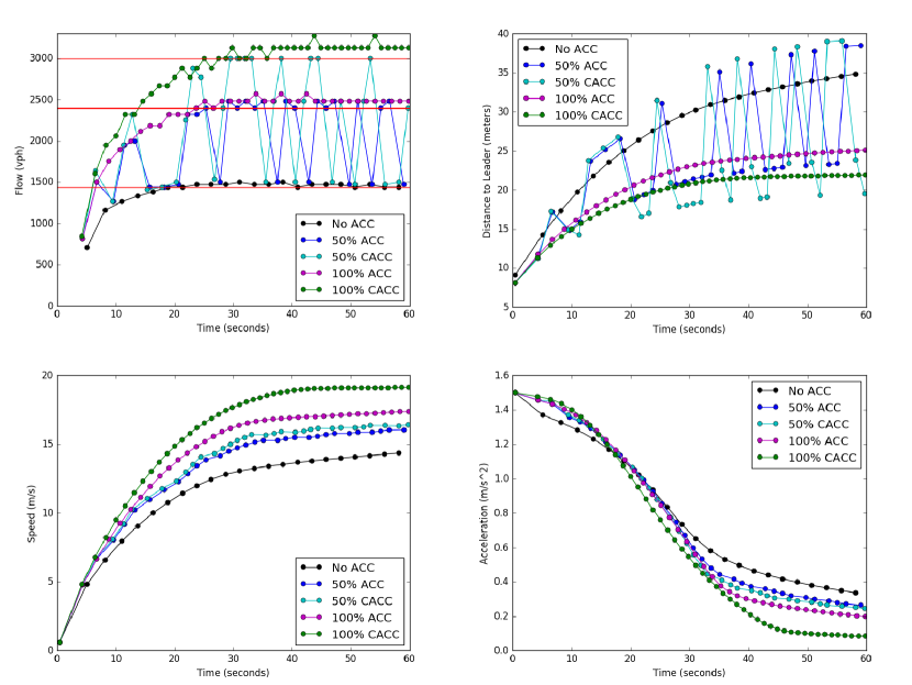
Figure 9: Single intersection case: comparison of point measurements of flow, distance to leader, speed and acceleration at the detector location for different portions of ACC/CACC traffic.

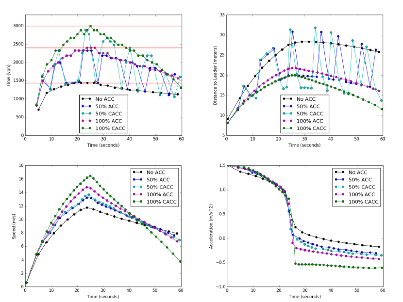
Figure 10: Case with red light downstream: comparison of point measurements of flow, distance to leader, speed and acceleration at the detector location for different portions of ACC/CACC traffic.

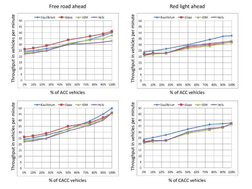
Figure 11: Intersection throughput as a function ACC/CACC portion of traffic computed with Gipps, IIDM and Helly car following models for two cases — free road downstream (left) and red light downstream (right).

We assume that the ACC vehicle has the same car following model as the ordinary one, just with different $\tau$ and $g_{\min}$. CACC vehicle behaves just as ACC, with ACC $\tau$ and $g_{\min}$, if it follows an ordinary vehicle, but if it has another CACC car in front, it assumes different car following behavior, which we call CACC car following model.

Denote $a_{IIDM}(t)$ the acceleration function defined by (2.4). Define constant-acceleration heuristic (CAH) acceleration function [43] (Chapter 11):

$$a_{CAH}(t)=\left\{\begin{array}[]{ll}\frac{v^{2}(t)\bar{a}_{l}(t)}{v_{l}^{2}(t)-2(x_{l}(t)-x(t)-l)\bar{a}_{l}(t)},&\mbox{ if }v_{l}(t)(v(t)-v_{l}(t))\leq-2(x_{l}(t)-x(t)-l)\bar{a}_{l}(t),\\ \bar{a}_{l}(t)-\frac{(v(t)-v_{l}(t))^{2}\Theta(v(t)-v_{l}(t))}{2(x_{l}(t)-x(t)-l)}&\mbox{ otherwise,}\end{array}\right.$$ (4.1)

where

$$\bar{a}_{l}(t)=\min\left\{\dot{v}_{l}(t),a_{\max}\right\},$$

and

$$\Theta(z)=\left\{\begin{array}[]{ll}1,&\mbox{ if }z\geq 0,\\ 0,&\mbox{ otherwise}.\end{array}\right.$$

Now we specify the CACC car following model [43] (Chapter 11):

$$a_{CACC}(t)=\left\{\begin{array}[]{ll}a_{IIDM}(t),&\mbox{ if }a_{CAH}(t)\leq a_{IIDM}(t),\\ a_{CAH}(t)+b\tanh\left(\frac{a_{IIDM}(t)-a_{CAH}(t)}{b}\right),&\mbox{ otherwise.}\end{array}\right.$$ (4.2)

As before, we run the free road and the red light downstream experiments using Gipps, IIDM and Helly car following models. For each of these models, we compute the intersection throughput, when portion of ACC (CACC) vehicles in the initial queue. Thus, we evaluate 72 cases, each defined by: (1) experiment — free road or red light downstream; (2) car following model — Gipps, IIDM, Helly; (3) ACC or CACC; and (4) percentage of ACC (CACC) — 10, 25, 50, 75, 90 and 100%.

Figures 9 and 10 compare flows, gaps, speeds and acceleration obtained at the detector location (see Figures 1 and 4) for 0, 50 and 100% ACC (CACC) penetration rate. Three horizontal red lines on flow plots in both figures correspond to equilibrium flows with 0% ACC (CACC), with 100% ACC and with 100% CACC penetration rate. These flows are computed as $3600/\theta_{e}$, where $\theta_{e}$ is given by (2.8) with $\tau$ and $g_{\min}$ from Table 5, yilding 1440, 2400 and 3000 vehicles per hour respectively. In the flow and distance to leader plots, one can see how 50% ACC curves jump between the no ACC and 100% ACC curves — for ordinary vehicles it is similar to the no ACC curve, and for an ACC vehicle it is similar to 100% ACC curve. 50% CACC curves in the same plots jump between three curves — no ACC, 100% ACC and 10% CACC. This is because a CACC vehicle following an ordinary one behaves like ACC vehicle.

For a given ACC (CACC) penetration rate less than 100%, the intersection throughput is sensitive to the distribution of ACC (CACC) vehicles in the initial queue. For example, if 25% all vehicles in the initial queue are ACC-enabled, and all of them are concentrated at the head of the queue, we would get higher vehicle count at the detector location after one minute, than we would with 50% ACC penetration rate when all ACC-enabled vehicles are concentrated at the tail of the queue. In another example, 50% CACC penetration rate would not produce any gain over 50% ACC penetration rate, if ordinary and ACC/CACC vehicles interleave — one ordinary, one ACC/CACC, one ordinary, and so on — since CACC provides benefit over ACC in terms of throughput only when some CACC vehicles have other CACC vehicles directly in front.

To mitigate this ACC (CACC) distribution bias, for each of the cases with ACC (CACC) penetration rate less than 100%, we run 100 one-minute simulations of the three car following models and record vehicle counts at the detector location, then take the median vehicle count. For 100% penetration rate the ACC (CACC) distribution is trivial, and hence, a single simulation for each case is enough. The intersection throughput results for all the 72 cases, together with throughput values from Table 3 obtained for 0 ACC (CACC) penetration rate, are presented at the four plots in Figure 11.

Note that in each of the four plots in Figure 11, in addition to the three curves corresponding to car following models, there is a curve corresponding to the equilibrium traffic flow. These equilibrium curves are computed as follows. Denote $\lambda\in[0,1]$ a portion of ACC (CACC) vehicles in the initial queue; $\tau^{[C]ACC}$ and $g_{\min}^{[C]ACC}$ the reaction time and minimal gap for ACC (CACC) vehicles, whose values are given in Table 5. The average headway in the equilibrium state is obtained by modifying expression (2.8):

$$\theta(\lambda)=\lambda\tau^{[C]ACC}+(1-\lambda)\tau+\frac{\lambda g_{\min}^{[C]ACC}+(1-\lambda)g_{\min}+l}{v_{\max}}.$$ (4.3)

Then, the equilibrium flow in vehicles per minute is given by:

$$f(\lambda)=60/\theta(\lambda).$$ (4.4)

This formula is sufficient for the case when there is a free road ahead. In the case of the red light downstream, however, we are restricted by the capacity of the link connecting the two intersections. To account for that, we modify (4.4) accordingly:

$$f(\lambda)=\min\left\{\frac{60}{\theta(\lambda)},\frac{k\Delta}{\lambda g_{\min}^{[C]ACC}+(1-\lambda)g_{\min}+l}\right\},$$ (4.5)

where $\Delta$ is the length of the link between the two intersections, and $k$ is the number of lanes in that link. In our experiment, $\Delta=300$, and $k=1$.

5 Platoon Model

Vehicles equipped with CACC technology can communicate with one another to form platoons. These platoons can increase the throughput of intersections by decreasing headways between successive vehicles. In simulation, platoon management and formation is divided into three phases:

1. identifying vehicles that can be grouped into platoons;

2. Adjusting parameters of leaders and followers in platoons; and

3. performing maintenance on the platoon.

This hierarchy is modeled by the state machine in Figure 12.

Figure 12: State machine describing platoon behavior.

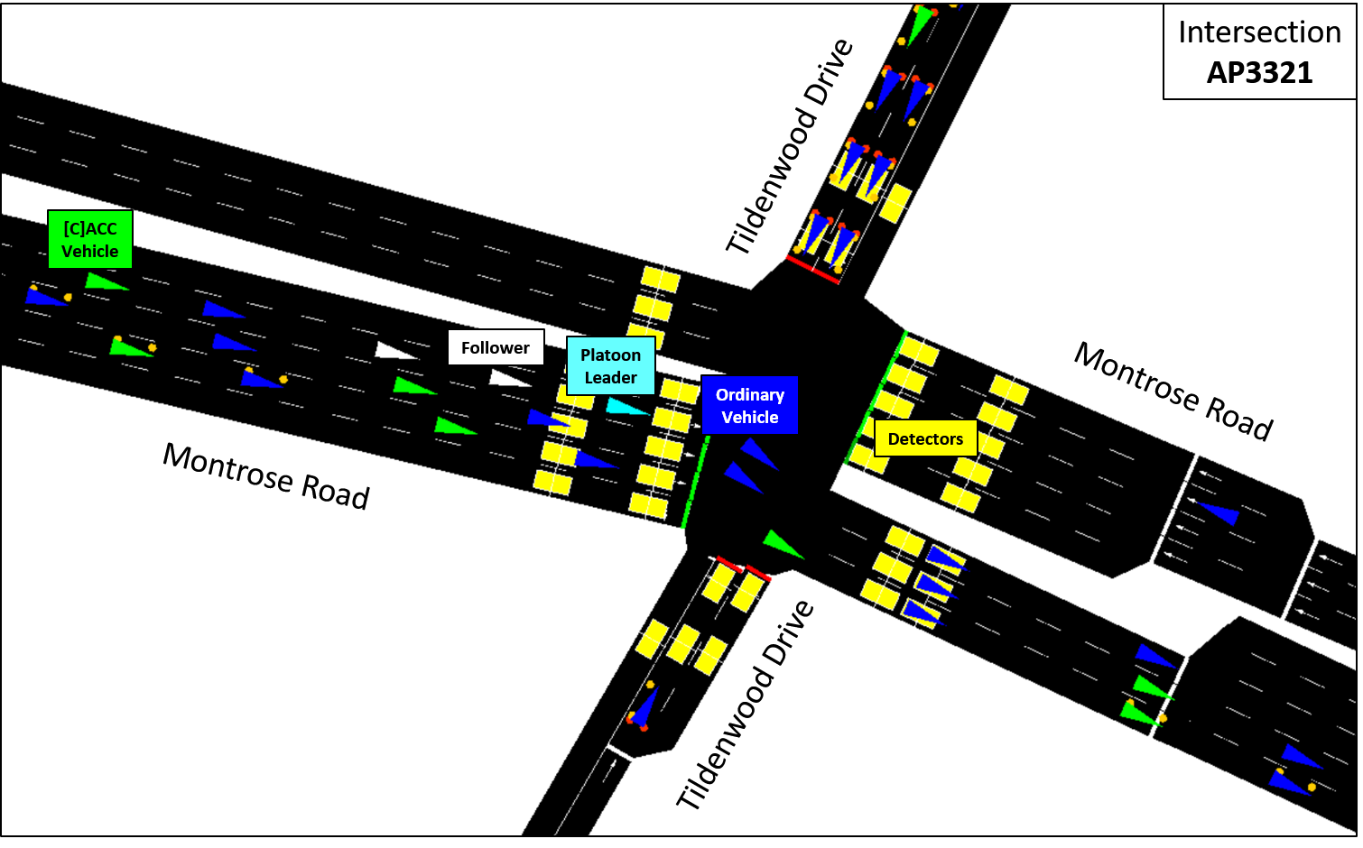
Figure 13: SUMO screenshot — ordinary, standalone [C]ACC vehicles and platoons are crossing intersection AP3321 (Montrose Road and Tildenwood Drive). Platoon leader and follower, as well as standalone [C]ACC and ordinary vehicles are labeled accordingly.

To form a platoon, vehicles must be in sequence with one another on a given lane. However, vehicles need not share the same final destination and are free to switch lanes or leave the platoon if necessary. If an intermediate vehicle in the platoon changes its route by making a turn or changing lanes, the platoon splits into two: one platoon for the vehicles ahead of the intermediate vehicle and another for all the vehicles behind.

A platoon’s lead vehicle has the same properties as ACC vehicles. An isolated CACC vehicle is a leader of a platoon of size 1. When a platoon leader comes into range of another CACC vehicle in front, it joins the platoon becoming a follower. Followers have reduced headway and travel much closer to one another than standalone vehicles. In addition, followers are able to receive information from the leader, such as to accelerate after a green light at an intersection or to decelerate approaching an obstacle, e.g. red light downstream.

Since followers are not bound to the same route as the platoon leader, they are free to separate. After leaving the platoon, the headway and acceleration parameters are restored to their original values. This can happen for example when the follower changes its route or becomes separated from the rest of platoon, e.g., due to switching traffic signal as it crosses the intersection.

Figure 13 displays a screenshot of SUMO simulation run in graphical mode. Ordinary vehicles are colored in blue. [C]ACC vehicles with no followers (standalone) are colored in green. Platoon leaders are colored in cyan, and followers are white.

Next, we discuss SUMO simulation results.

6 Case Study: Simulation of North Bethesda Road Network

To study the impact of platooning, we built the SUMO [25] simulation model of the North Bethesda network with seven major intersections, shown in Figure 14. IIDM and CACC car following models were implemented in C++ within SUMO, and platoon management, presented as a state machine in Figure 12, was implemented in Python using SUMO/TraCI API [2]. The corresponding source code repository can be accessed at [1].

Using vehicle counts and estimated turn ratios, we generated 1 hour of origin-destination (O-D) travel demand data with a route assigned to each vehicle. These travel demand data together with signal plans constitute input for the simulation model.

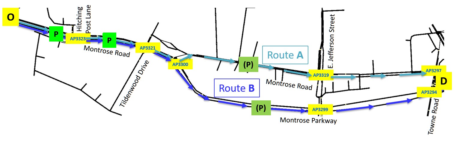
Figure 14: North Bethesda network — O-D pair with routes A and B. Labels ‘P’ indicate links, where platoons form, when platooning is enabled. Labels ‘(P)’ indicate additional links with optional platooning, when it is enabled.

We focused our study on the single O-D pair with two routes, A and B, connecting origin (O) and destination (D) — see Figure 14. Routes A and B coincide in the beginning, following Montrose Road, and split at intersection AP3300 into Montrose Road (route A) and Montrose Parkway (route B).

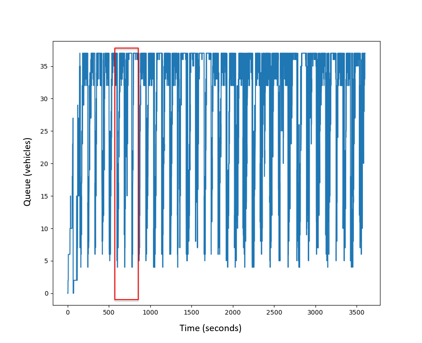
Figure 15: Queue dynamics at the route A (B) approach to the intersection of Montrose Road and Hitching Post Lane (AP3323).

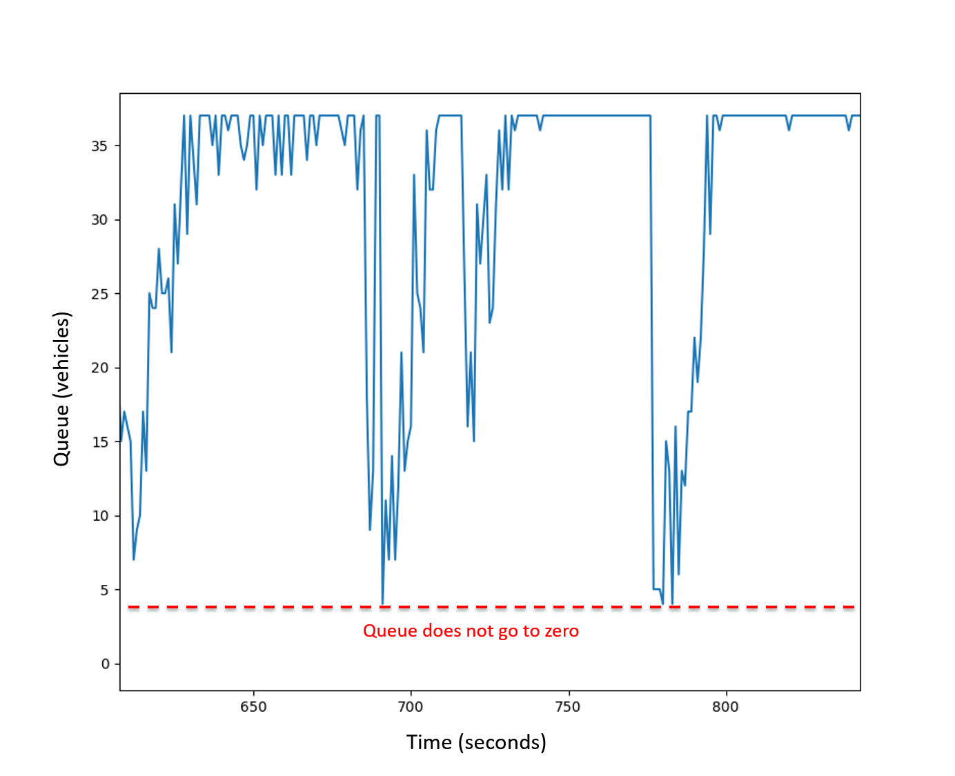
Figure 16: Zoomed-in queue dynamics from Figure 15 — queue does not empty.

General approach to congestion analysis on an arterial network is as follows. Intersections, where under a given demand a vehicle queue on at least one approach keeps growing are identified as bottlenecks. If rearranging the duration of green phases within a cycle leads to a periodic queue behavior — when a queue grows then dissolves — on all intersection approaches, then this intersection bottleneck is due to poor control. If, on the other hand, with any phase split we continue observing at least one increasing queue, then we have a situation of excessive demand.

Figures 15-16 show queue dynamics at the routes A and B approach to the intersection of Montrose Road and Hitching Post Lane (AP3323). Vehicle queue measured in SUMO does not grow beyond the storage capacity of a road link, where this queue is measured. Once the link storage capacity is reached, queue spills back into the upstream link. In Figures 15-16, queue size reaches the storage capacity of 36. Actually, it grows further, but SUMO reports only the maximum halted vehicles in this particular link. What we observe from the queue dynamnics plot, though, is that after a certain time peiod, this vehicle queue is never fully served. In other words, number of vehicles in the queue does not go to zero. It means, that green phase for the vehicles on routes A and B at intersection AP3323 is too short for the given demand. It so happens that increasing green phase for the movement corresponding to routes A and B is not a viable option, because that would create a backup on the cross street, Hitching Post Lane. Thus, we have a case of excessive demand at intersection AP3323. The problem of excessive demand may be mitigated with decreasing vehicle headways — through platoon creation.

We enabled platooning on two links labeled ‘P’ in Figure 14 — upstream and downstream links of intersection AP3323 on routes A and B. Then, we ran a series of simulation scenarios varying the fraction of ACC (CACC) vehicles from 0 to 75%. In each simulation two vehicle classes were modeled: ordinary vehicles and ACC (or CACC) vehicles. In simulations with CACC vehicles platoons were formed in those two links, where platoning was enabled. The same number of vehicles was processed in each simulation. The rates and locations at which cars were generated were identical in all scenarios to eliminate the variance in randomly generated routes. For cases of 0, 25, 50 and 75 percent ACC (CACC) penetration rate, we computed average travel time for routes A and B. Table 6 lists the resulting mean travel times.

[C]ACC %	Vehicle Class	Route A		Route B
		ACC	CACC	ACC	CACC
0	ordinary	711	711	622	622
25%	ordinary	696	696	608	607
	[C]ACC	691	688	604	598
	all	695	694	607	605
50%	ordinary	671	670	553	547
	[C]ACC	665	646	539	523
	all	671	658	546	535
75%	ordinary	661	646	526	516
	[C]ACC	660	642	526	509
	all	660	643	526	511

Table 6: Mean travel time in seconds for varying percentage of [C]ACC vehicles on routes A and B (see Figure 14).

We can see that ACC vehicles alone (without platooning) reduce the travel time along both routes A and B. Travel time improvement achieved by CACC over ACC should be attributed to the higher throughput of intersection AP3323, resulting in smaller queues and thus, smaller waiting times in queues, formed upstream of this intersection. Note that ordinary vehicles show reduced travel times, although [C]ACC vehicles have larger gains. Another observation is that the biggest travel time improvement happens when CACC penetration rate goes from 25 to 50%. The reason is that with 25% CACC penetration rate, chances that CACC vehicles will be positioned in sequence, so that a platoon can be formed, are relatively low. So, CACC case does not show much improvement over ACC with 25% penetration rate. On the other hand, when CACC peneration rate is high at 75%, platoons become much more frequent and of larger sizes. This leads to oversaturation of the downstream link, creating a new bottleneck that offsets some of the upstream travel time gains achieved by the platooning.

CACC %	Vehicle Class	Route A		Route B
		Original	Additional Platooning	Original	Additional Platooning
25%	ordinary	696	695	607	607
	CACC	688	686	598	599
	all	694	693	605	605
50%	ordinary	670	672	547	548
	CACC	646	644	523	520
	all	658	658	535	534
75%	ordinary	646	646	516	515
	CACC	642	641	509	506
	all	643	642	511	508

Table 7: Comparing mean travel time on routes A and B from the original platooning experiment with the mean travel time, where platooning is allowed in the additional links, as indicated in Figure 14. Travel time is in seconds.

To see how platooning can further reduce trave times on routes A and B, we enabled it on links approaching intersections AP3319 (on route A) and AP3299 (on route B). Those additional platooning links are labeled ‘(P)’ in Figure 14. Then, we re-ran simulation scenarios with 25, 50 and 75% [C]ACC portion of traffic. Average travel times for routes A and B are summarized in Table 7, comparing them with the results of the original experiment.

As we can see, additional platooning practically does not reduce travel time. This happens because intersections AP3319 and AP3299 are not bottlenecks, Pushing vehicles through these intersection in platoons does not qualitatively change queue dynamics at AP3319 and AP3299 on routes A and B: the green phase was sufficient to handle unplatooned traffic.

Moreover, platooning may cause a problem on cross streets. In the case of 50% CACC penetration rate, platooning pushes too much traffic through intersection AP3319 along route A blocking the link downstream of this intersection for the left-turning traffic from E. Jefferson Street. SUMO screenshot depicting this situation is presented in Figure 17.

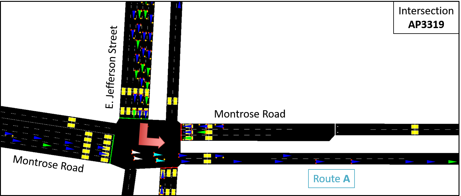
Figure 17: Intersection AP3319 — jam at E. Jefferson Street left turn pocket.

Thus, we can succinctly formulate the platooning rule:
platooning should be enabled only at the approaches to bottleneck intersections.

7 Conclusion

Analysis of the Gipps, IIDM and Helly car following models shows that:

• Theoretical bound on intersection throughput defined by the equilibrium flow may be exceeded in the case of accelerating traffic — slower speed is compensated by a larger traffic density.

• Gipps model exhibits too aggressive acceleration behavior, and, if used for estimation of intersection throughput, may produce unrealistically high vehicle counts, which, in the case of free road downstream, exceed the theoretical bound.

• Helly model produces deceleration profile that is unacceptable for drivers and passengers, which makes it not suitable for quantitative assessment of intersection throughput.

• Acceleration of IIDM is more gradual than that of Gipps, and deceleration is more gentle than that of both Gipps and Helly. IIDM suits better for the analysis of ACC/CACC impact on the arterial throughput than the other two models.

Presence of ACC-enabled vehicles in the traffic increases the intersection throughput and improves travel time. The impact of CACC-enabled vehicles that can form platoons largely depends on how vehicles are ordered in the traffic stream: CACC vehicles forming a sequence can increase the flow through intersection significantly more than can be achieved with pure ACC vehicles; while CACC vehicles interleaved with ordinary ones have the same effect as pure ACC vehicles.

Ordering of vehicles matters not only in the presence of CACC, but even just ACC vehicles. Grouped closer to the head of the queue ACC (CACC) vehicles increase the intersection throughput more than if they were in the queue’s tail. CACC vehicles interleaved with ordinary ones have the same effect as ACC vehicles.

In an urban network the presence of (C)ACC vehicles reduces the queues and hence the time spent at intersections. As a result ordinary as well as (C)ACC vehicles benefit from lower average travel times.

Platooning helps at bottleneck intersections, where bottleneck cannot be dissolved by changing signal cycle and splits. Platooning may be harmful in the following cases:

• downstream intersection is a bottleneck;

• downstream intersection can become a bottleneck as a result of increased throughput going there; and

• flows from other approaches at current intersection can be blocked.

References

- [1] Sustainable Operation of Arterial Networks: Source Code Repository. http://github.com/ucbtrans/sumo-project.
- [2] Traffic Control Interface (TraCI) for SUMO. http://sumo.dlr.de/wiki/TraCI.
- [3] M. Abbas, D. Bullock, and L. Head. Real-time offset transitioning algorithm for coordinatinng traffic signals. Transportation Research Record, 1748:26–39, 2001.
- [4] R. Azimi, G. Bhatia, R. Rajkumar, and P. Mudalige. Reliable intersection protocols using vehicular networks. In Proc. 2013 ACM/IEEE International Confernce on Cyber-Physical Systems (ICCPS), pages 1–10, Philadelphia, PA, 2013. IEEE.
- [5] R. Azimi, G. Bhatia, R. Rajkumar, and P. Mudalige. Ballroom intersection protocol: Synchronous autonomous driving a intersections. In Proc. 21st International Conference on Embedded and Real-Time Computing Systems and Applications, pages 167–215, Hong Kong, 2015. IEEE.
- [6] H. Bai, H. Liu, Y. Zhao, and N. Wang. Length otimization of traffic signal cycle. International Journal of Advancements in Computing Technology, 4(4):156–164, 2012.
- [7] M. Bando, K. Hasebe, A. Nakayama, A. Shibata, and Y. Sugiyama. Dynamical model of traffic congestion and numerical simulation. Physical Review E, 51:1035–1042, 1995.
- [8] M. Brackstone and M. McDonald. Car-following: A historical review. Transportation Research, Part F: Traffic Psychology, 2(4):181–196, 1999.
- [9] R. E. Chandler, R. Herman, and E. W. Montrol. Traffic dynamics: Studies in car-following. Operations Research, 6:165–184, 1958.
- [10] G. De Nunzio, G. Gomes, C. Canudas de Wit, R. Horowitz, and P. Moulin. Arterial bandwidth and energy consumption optimization via signal offsets control and variable speed limits. In IEEE Conference on Decision and Control, 2015.
- [11] C. Diakaki, V. Dinopoulou, K. Aboudolas, M. Papageorgiou, E. Ben-Shabat, E. Seider, and A. Leibov. Extensions and new applications of the traffic-responsive urban control strategy. Transportation Research Record, 1856:202–211, 2003.
- [12] P. Fernandes and U. Nunes. Platooning leaders positioning and cooperative behavior algorithms of communicaant automated vehicles for high traffic capacity. IEEE Transactions on Intelligent Transportation Systems, 16(3):1172–1187, 2015.
- [13] H.T. Fritzsche. A model for traffic simulation. Traffic Engineering and Control, (5):317–321, 1994.
- [14] N. Gartner, S. Assman, F. Lasaga, and D. Hou. A multi-band approach to arterial traffic signal optimization. Transportation Research, Part B, 25(1):55–74, 1991.
- [15] N. Gartner and C. Stamadiadis. Arterial-based control of traffic flow in urban grid networks. Mathematical and Computer Modelling, 35:657–671, 2002.
- [16] D. C. Gazis, R. Herman, and R. W. Rothery. Nonlinear follow-the-leader models of traffic flow. Operations Research, 9:545–567, 1961.
- [17] P. G. Gipps. A behavioral car-following model for computer simulation. Transportation Research, Part B: Methodological, 15(2):105–111, 1981.
- [18] D. Godbole, M. A. Kourjanski, R. Sengupta, and M. Zandonadi. Breaking the highway capacity barrier: Adaptive cruise control-based concept. Transportation Research Record, 1679:148–157, 1999.
- [19] G. Gomes. Bandwidth maximization using vehicle arrival functions. IEEE Transactions on Intelligent Transportation Systems, 16(99):1–12, 2015.
- [20] W. Helly. Simulation of bottlenecks in single lane traffic flow. In Proceedings of International Symposium on the Theory of Traffic Flow, New York, NY, 1959.
- [21] S. Hoogendoorn, S. Ossen, and M. Schreuder. Empirics of multianticipative car-following behavior. Transportation Research Record, 1965:112–120, 2006.
- [22] R. Jiang, Q. Wu, and Z. Zhu. Full velocity difference model for a car-following theory. Physical Review E, 64(1):017101, 2001.
- [23] A. Kesting, M. Treiber, and D. Helbing. Enhanced intelligent driver model to access the impact of driving strategies on traffic capacity simulations. Philosophical Transactions of the Royal Society A, 368:4585–4605, 2010.
- [24] K.B. Kesur. Optimization of mixed cycle length traffic signals. Journal of Advanced Transportation, 48(5):431–442, 2012.
- [25] D. Krajzewicz. Traffic simulation with sumo-simulation of urban mobility. In Fundamentals of Traffic Simulation, pages 269–293. Springer, 2010. http://www.dlr.de/ts/en/desktopdefault.aspx/tabid-9883/16931_read-41000, accessed 04/28/2016.
- [26] S Krauss. Microscopic Modeling of Traffic Flow: Investigation of Collision Free Vehicle Dynamics. Phd thesis, Hauptabteilung Mobilität und Systemtechnik, Cologne, 1998.
- [27] A. A. Kurzhanskiy and P. Varaiya. Traffic management: An outlook. Economics of Transportation, 4(3):135–146, 2015.
- [28] J. Lioris, R. Pedarsani, F. Y. Tascikaraglu, and P. Varaiya. Platoons of connected vehicles can double throughput in urban roads. Submitted to Transportation Research, Part C: Emerging Technologies, 2015. https://arxiv.org/abs/1511.00775.
- [29] J. Little. The synchronizing traffic signals by mixed-integer linear programming. Operations Research, 14:896–912, 1965.
- [30] V. Milanés, S.E. Shladover, J. Spring, C. Nowakowski, H. Kawazoe, and M. Nakamura. Cooperative adaptive cruise control in real traffic situations. IEEE Transactions on Intelligent Transportation Systems, 15(1):296–305, 2014.
- [31] J. Morgan and J. Little. Synchronizing traffic signals for maximum bandwidth. Operations Research, 12(6):896–912, 1964.
- [32] G. F. Newell. Nonlinear effects in dynamics of car following. Operations Research, 9(2):209–229, 1961.
- [33] G. F. Newell. A simplified car-following theory: A lower order model. Transportation Research, Part B: Methodological, 36:195–205, 2002.
- [34] N. Papola and G. Fusco. Maximal bandwidth problem: A new algorithm based on the property of periodicity of the system. Transportation Research, Part B, 32(4):277–288, 1998.
- [35] R. Pillai, A. Rathi, and S. Cohen. A restricted branch-and-bound approach for generating maximum bandwidth signal timing plans for traffic networks. Transportation Research, Part B, 32(8):517–529, 1998.
- [36] L. A. Pipes. An operational analysis of traffic dynamics. Journal of Applied Physics, 24:274–281, 1953.
- [37] A. Reuschel. Fahrzeugbewegungen in der kolonne. Oesterreichisches Ingenieur-Archiv, 4:193–215, 1950.
- [38] W. J. Schakel, B. van Arem, and B. Netten. Effects of cooperative adaptive cruise control on traffic flow stability. In Proceedings of the 13th IEEE Conference on Intelligent Transportation Systems, Madeira Island, Portugal, September 2010.
- [39] D. Schrank, B. Eisele, and T. Lomax. 2015 Urban Mobility Report Scorecard. Technical report, Texas Transportation Institute, 2015. http://mobility.tamu.edu.
- [40] M.J. Smith, R. Liu, and R. Mounce. Traffic control and route choice; capacity maximization and stability. Transportation Research, Part B. In Press., 2015.
- [41] D. Swaroop. String Stability in Interconnected Systems: An Application to a Platoon of Vehicles. Phd thesis, University of California, Berkeley, 1994.
- [42] M. Treiber, A. Hennecke, and D. Helbing. Congested traffic states in empirical observations and microscopic simulations. Physical Review E, 62(2):1805–1824, 2000.
- [43] M. Treiber and A. Kesting. Traffic Flow Dynamics: Data, Models and Simulation. Springer, 2013.
- [44] B. van Arem, C. J. G. van Driel, and R. Visser. The impact of cooperative adaptive cruise control on traffic flow characteristics. IEEE Transactions on Intelligent Transportation Systems, 7(4):429–436, 2006.
- [45] J. VanderWerf, S. Shladover, M. Miller, and N. Kourjanskaia. Effects of adaptive cruise control systems on highway traffic flow capacity. Transportation Research Record, 1800:78–84, 2002.
- [46] P. Varaiya. Smart cars on smart roads:problems of control. IEEE Transactions on Automatic Control, 38(2):195–207, 1993.
- [47] P. Varaiya. The max-pressure controller for arbitrary networks of signalized intersections. In S.V. Ukkusuri and K. Ozbay, editors, Advances in Dynamic Network Modeling in Complex Transportation Systems, volume 2 of Complex Networks and Dynamic Systems. Springer, 2013.
- [48] M. Wang, M. Treiber, W. Daamen, S. P. Hoogendorn, and B. van Arem. Modelling supported driving as an optimal control cycle: Framework and model characteristics. 20th International Symposium on Transportation and Traffic Theory (ISTTT), 80(7):491–511, 2013.
- [49] R. Wiedemann. Simulation des Strassenverkehrflusses. PhD thesis, Universtät Karlsruhe, Band 8, Karlsruhe, Deutschland, 1974.
- [50] R. Wiedemann and U. Reiter. Microscopic traffic simulation: the simulation system mission, background and actual state. Final report, Project ICARUS, Brussels, 1992.