An overabundance of low-density Neptune-like planets

Abstract

We present a uniform analysis of the atmospheric escape rate of Neptune-like planets with estimated radius and mass (restricted to $M_{\rm p}<30\,M_{\oplus}$). For each planet we compute the restricted Jeans escape parameter, $\Lambda$, for a hydrogen atom evaluated at the planetary mass, radius, and equilibrium temperature. Values of $\Lambda\lesssim 20$ suggest extremely high mass-loss rates. We identify 27 planets (out of 167) that are simultaneously consistent with hydrogen-dominated atmospheres and are expected to exhibit extreme mass-loss rates. We further estimate the mass-loss rates ($L_{\rm hy}$) of these planets with tailored atmospheric hydrodynamic models. We compare $L_{\rm hy}$ to the energy-limited (maximum-possible high-energy driven) mass-loss rates. We confirm that 25 planets (15% of the sample) exhibit extremely high mass-loss rates ($L_{\rm hy}>0.1\,M_{\oplus}{\rm Gyr}^{-1}$), well in excess of the energy-limited mass-loss rates. This constitutes a contradiction, since the hydrogen envelopes cannot be retained given the high mass-loss rates. We hypothesize that these planets are not truly under such high mass-loss rates. Instead, either hydrodynamic models overestimate the mass-loss rates, transit-timing-variation measurements underestimate the planetary masses, optical transit observations overestimate the planetary radii (due to high-altitude clouds), or Neptunes have consistently higher albedos than Jupiter planets. We conclude that at least one of these established estimations/techniques is consistently producing biased values for Neptune planets. Such an important fraction of exoplanets with misinterpreted parameters can significantly bias our view of populations studies, like the observed mass–radius distribution of exoplanets for example.

1 INTRODUCTION

The Kepler Space Telescope mission has enabled the first estimations of the abundance and size distribution of extrasolar planets in our galaxy (e.g., Fressin et al., 2013; Dressing & Charbonneau, 2015). A large fraction of these worlds have sizes intermediate between that of Earth and Neptune, having no analog in our solar system. Further follow-up studies have yielded mass estimates for a large sample of Neptune-like planets (hereafter, considered as those planets with $M_{\rm p}<30{M_{\oplus}}\,\approx 2M_{\rm Nep}$), allowing us to study the physical properties of exoplanets in a statistically robust manner.

The planetary radius is inferred from optical transit light-curve observations, typically corresponding to the $\sim 20-100$ mbar level for a clear atmosphere (e.g., Lopez & Fortney, 2014; Lammer et al., 2016; Lecavelier des Etangs et al., 2008). The planetary mass, in turn, is inferred either from measurements of the stellar radial velocity (RV) or from transit timing variations (TTV) due to interplanetary perturbations. By combining the mass and radius constraints, we can infer bulk densities and compositions. For a given mass, the planetary radius does not significantly depend on the interior composition, since it is made of very incompressible materials. On the contrary, for a given mass, the hydrogen envelope fraction strongly correlates with the planetary radius (Lopez & Fortney, 2014).

The mass–size distribution shows that a considerable fraction of Neptune-like planets have significant envelopes (a few percent of the core mass). Noteworthy, a couple dozen of sub Neptunes show bulk densities far lower than that of the solar-system giant planets. While it is plausible that solid cores of a few $M_{\oplus}$ can accrete significant gas envelopes before the protoplanetary disk dissipation (Lee et al., 2014; Inamdar & Schlichting, 2015; Stökl et al., 2016; Ginzburg et al., 2016), several studies find that after the disk dispersal these gas envelopes endure significant mass loss due to different mechanisms.

Cooling and photoevaporation, driven by the high-energy stellar irradiation (XUV), produce moderate mass-loss rates and atmospheric contraction. These mechanisms act over timescales larger than $\sim 10^{8}$ yr (e.g., Lopez et al., 2012; Owen & Wu, 2013; Ginzburg et al., 2016). Hydrodynamic and photochemical processes determine the composition of the upper atmosphere of these planets, and therefore of the escaping particles Koskinen et al. (e.g., 2013a, b)

Using hydrodynamic simulations, Owen & Wu (2016) found that during the first $\sim$Myr after the disk dispersal, low-density planets exhibit extremely high thermally driven mass-loss rates, dubbed “boil-off” (see also Lammer et al., 2016; Fossati et al., 2016). This mechanism consists of hydrodynamic thermal evaporation (Parker wind), driven by the internal heat from the planet, and fueled by the stellar continuum irradiation. During this regime, the atmosphere quickly cools and contracts as it releases energy through the escaped particles. In other words, the thermal energy exceeds the gravitational energy in atmospheric layers where the density is high enough to lead to high mass-loss rates. Consequently, the mass-loss rate exponentially decays until the XUV-driven photoevaporation becomes the dominant mass-loss mechanism (Stökl et al., 2015).

The extremely high mass-loss rates of this regime are unsustainable for the atmospheres of Neptune-like planets over Gyr timescales. Therefore, only young systems are expected to show thermally driven mass-loss rates in excess of the XUV-driven mass-loss rates (Lammer et al., 2016).

Ultraviolet transit observations provide evidence of mass loss on exoplanets (e.g., Vidal-Madjar et al., 2003; Linsky et al., 2010; Fossati et al., 2010; Ben-Jaffel & Ballester, 2013). For example, Ly-$\alpha$ transit observations (e.g., Vidal-Madjar et al., 2003; Kulow et al., 2014; Ehrenreich et al., 2015; Bourrier et al., 2016) show transit depths much larger than in the optical. These observations are interpreted as absorption from an extended region of escaping gas beyond the Roche lobe of the planet.

However, the translation from observations into mass-loss rates is very model-dependent. Ly-$\alpha$ observations show large offsets between the absorption features and the center of the line ($\pm 100$ km s^-1), requiring additional assumptions to explain the observations. Among the proposed mechanisms there are: natural broadening from large-scale confinement of material into a higher-density region (Stone & Proga, 2009; Owen & Adams, 2014), a combination of stellar radiation pressure and wind interactions, where particles accelerate by charge exchange in the wind-wind interaction region (Holmström et al., 2008; Tremblin & Chiang, 2013; Kislyakova et al., 2014; Christie et al., 2016), or inhomogeneities of the stellar disc at Ly-$\alpha$ light (Llama et al., 2013).

1.1 Restricted Jeans Escape Parameter

Fossati et al. (2016) described the thermal escape in terms of the classical Jeans escape parameter (see e.g., Chamberlain & Hunten, 1987). They generalized the Jeans escape parameter for a hydrodynamic atmosphere subjected to the gravitational perturbation from the host star. They studied the upper atmosphere, between the 100 mbar level and the Roche-lobe radius, using hydrodynamic models. By deriving the generalized Jeans escape parameter across the atmospheric layers, they were able to determine how stable a planetary atmosphere is against evaporation.

Fossati et al. (2016) further defined the restricted Jeans escape parameter:

$${\Lambda}\equiv\frac{GM_{\rm p}m_{H}}{k_{B}{T_{\rm eq}}R_{\rm p}},$$ (1)

the Jeans escape parameter for a hydrogen atom evaluated at the planetary mass ($M_{\rm p}$), radius ($R_{\rm p}$), and equilibrium temperature (${T_{\rm eq}}$), where $m_{\rm H}$ is the mass of the hydrogen atom, $G$ is the gravitational constant, and $k_{B}$ is the Boltzmann constant. For hydrogen-dominated atmospheres, $\Lambda$ is an easy-to-calculate parameter that allows one to estimate when the hydrodynamic mass-loss rate exceeds the XUV-driven photoevaporation.

We note that, whereas the classical Jeans escape parameter is a variable as function of altitude in an atmosphere, our definition of $\Lambda$ is a particular value of it that works as a global parameter for a given planet (no altitude dependence). This is similar to the definition of Guillot et al. (1996), but evaluated at the planetary equilibrium temperature. Using this specific definition, we empirically found the boil-off threshold at $\Lambda\sim 20$ (Fossati et al., 2016), equivalent to the threshold of $R=0.1R_{\rm Bondi}$ of Owen & Wu (2016).

Fossati et al. (2016) determined that planets with ${\Lambda}\lesssim 20$–$40$ should be experiencing extreme mass-loss rates by comparing the hydrodynamic escape rate, $L_{\rm hy}$, to the maximum XUV-driven escape rate, $L_{\rm en}$ (estimated through the energy-limited formula, Watson et al., 1981), over a range of $\Lambda$ scenarios with varying stellar type, planetary mass, and planetary radius.

In this paper we follow up the studies of atmospheric escape, modeling and estimating the present-day mass-loss rates for a sample of known exoplanets. We compile a list of the exoplanets with estimated masses and radii, and calculate their restricted Jeans escape parameter, $\Lambda$ (Section 2). Then, we compute hydrodynamic models tailored for planets suspected of being in the boil-off regime (Section 3). Finally we discuss the observational and physical implications of our findings (Section 4).

2 SAMPLE OF KNOWN NEPTUNES

We compiled our sample by collecting and crosschecking the lists of exoplanets from the Nasa Exoplanet Archive the Exoplanets Data Explorer (Han et al., 2014), and The Extrasolar Planets Encyclopaedia (Schneider et al., 2012). We selected the targets with measured planetary radii and masses, whose mass is less than $\sim 2$ Neptune masses ($M_{\rm p}<30~{}M_{\oplus}$). We adopted stellar rotational angular velocity ($\Omega_{\rm rot}$) from McQuillan et al. (2013) and ages from Morton et al. (2016). Our final sample consists of 167 planets (Table 2).

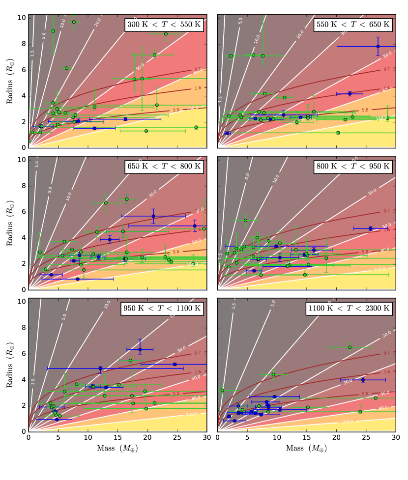
Figure 1: Mass–radius–$T$eq distribution of the known Neptune-like planets. The blue and green markers denote RV- and TTV-measured masses, respectively. From top to bottom, the brown solid lines denote constant-density curves corresponding to Saturn’s, Neptune’s, and Earth’s bulk density in g cm^-3, respectively. The background color contour denotes the value of $\Lambda$ for the mean equilibrium temperature of the planets in each panel: 455, 600, 715, 870, 1025, and 1440 K. Note that the $\Lambda$-contours work only as a guideline, Table 2 gives the specific values for each planet.

Fig. 1 shows the mass–radius–$T$eq distribution for the planets in this sample. We calculated the equilibrium temperature assuming zero Bond albedo and efficient day–night energy redistribution. We split this figure into temperature bins to show representative $\Lambda$ contours for the planets.

This is a heterogeneous sample of planets. The large majority of these planets (90% of the sample) were discovered using the transit method from the Kepler Space Telescope. The masses of these planets were estimated using the TTV and RV methods (70% and 30% of the sample, respectively), with only a few systems having both TTV and RV constraints: Kepler-18, Kepler-89, K2-19, and WASP-47.

The distribution of planets in Fig. 1 reflects the selection biases from each observing method. Most RV planets fall into the two panels with higher $T$eq because the RV method favors planets orbiting closer to their host stars. Furthermore, for a given planet size, the RV method tends to find planets with higher mass while the sensitivity of TTVs is more uniform (Weiss & Marcy, 2014; Steffen, 2016). Jontof-Hutter et al. (2014) argued that larger planets have deeper transits yielding more precise transit times.

Table 2 lists the observed and derived parameters for each planet. We selected the planets consistent with an envelope mass fraction larger than 1% (88 planets) by comparing the observed radii to the models of Lopez & Fortney (2014), for the given planetary masses, stellar ages, and incident fluxes. From this sub sample, we identify 28 planets (17% of the sample) with ${\Lambda}<20$, and thus should exhibit extreme mass-loss rates. We note that all of these systems are old ($>$1 Gyr). We observe some exceptional cases in system parameters, extremely low-bulk-density planets ($\rho_{\rm p}<0.2$ g cm^-3) like Kepler-33, Kepler-51, Kepler-79, Kepler-87, or Kepler-177; and extremely unstable atmospheres (${\Lambda}<5$) like Kepler-33 c or Kepler-51 b.

3 HYDRODYNAMIC RUNS

In this section we present hydrodynamical models of the upper atmosphere of selected Neptune-like planets, which allow us to directly estimate the present-day hydrodynamic mass-loss rate. We further determine whether their mass-loss rate is higher than the upper-limit XUV-driven mass-loss rate. We covered a range of $\Lambda$ from 0 to 50, including all hydrogen-dominated atmospheres with ${\Lambda}<20$, some higher-density planets, and some planets with larger $\Lambda$.

To compute $L_{\rm hy}$, we applied the one-dimensional upper-atmosphere hydrodynamic model of Erkaev et al. (2016). This model solves the hydrodynamic system of equations for mass, momentum, and energy conservation, considering the absorption of stellar XUV flux and accounting for the particles’ ionization, dissociation, recombination, and Ly-$\alpha$ cooling.

For the XUV absorption we assume a spherically symmetric distribution of density, deviations from this symmetry do not seem to be essential. One could expect that difference between 1D and 3D models would be more pronounced for cases of larger Jeans escape parameter, when the hydrodynamic flow is driven mainly by the XUV flux, which may have strong asymmetries. But in such case the mass-loss rate is rather close to the energy-limited escape value, as observed in existing 2D (Khodachenko et al., 2015) and 3D (Tripathi et al., 2015) simulations.

For hot Jupiters, our model produces similar mass-loss rates as most other hydrodynamic models (Erkaev et al., 2016). For the Neptune-like planet GJ 436 b, our model predicts a mass-loss rate of $2$$\times$$10^{-9}$ g s^-1, consistent with the values from Ehrenreich et al. (2015).

As in Tu et al. (2015) and Johnstone et al. (2015), we calculate the stellar X-ray and EUV luminosities using the scaling laws of Wright et al. (2011) to convert the stellar rotation rates and masses into X-ray luminosities, and Sanz-Forcada et al. (2011) to convert the X-ray luminosities into EUV luminosities. When the stellar rotation rate is not known, we use the gyrochronological relation of Mamajek & Hillenbrand (2008) to convert stellar age into rotation rate.

We calculate the upper-limit XUV-driven escape using the energy-limited formula (Watson et al., 1981; Erkaev et al., 2007):

$$L_{\rm en}=\frac{\pi\eta R_{\rm p}(R_{\rm XUV}^{\rm eff})^{2}F_{\rm XUV}}{GM_{\rm p}m_{H}K},$$ (2)

with $\eta=15$% the net heating efficiency (Shematovich et al., 2014), $R_{\rm XUV}^{\rm eff}$ the radius where the bulk of the XUV energy is absorbed, and $K$ the potential energy reduction factor due to stellar tides, which depends on the Roche-lobe boundary radius.

It is important to remark that both the stellar flux and the planetary parameters vary over their respective lifespan, inducing a variation in the planetary mass-loss rate with time (see, e.g., Lecavelier des Etangs et al., 2004; Lecavelier Des Etangs, 2007). In particular, for the boil-off regime, Owen & Wu (2016) argue that the mass-loss rate is exponentially sensitive to the planetary radius at small $\Lambda$. Thus, during boil-off, strong cooling and contraction quickly reduce $R_{\rm p}$ (and hence ${L_{\rm hy}}$) in timescales of $\sim 1$ Myr until $\Lambda\sim 20$. The XUV stellar fluxes we compute take into account the age of the star, whereas the planetary radii and masses are taken directly from the reported values. Therefore, the mass-loss rates we compute should be considered as a present-day snapshot of their values.

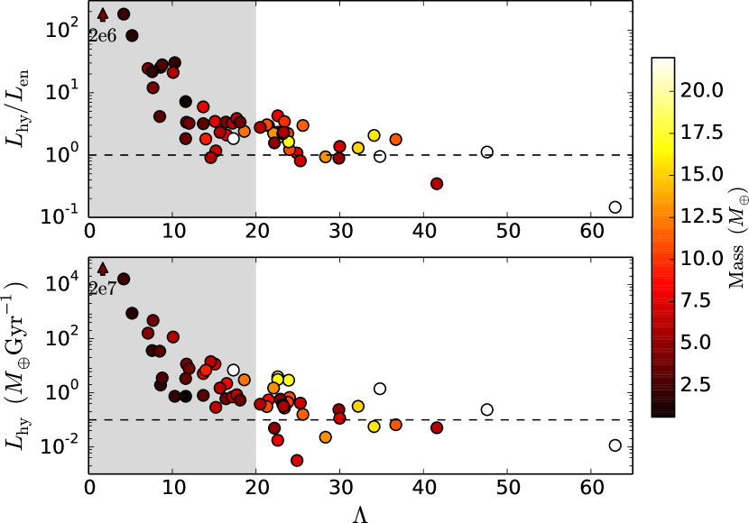
Figure 2: Top: Ratio between the hydrodynamic and energy-limited mass-loss rate vs. $\Lambda$. The color scale denotes the planetary mass. The background color marks the regions with dominant extreme thermal mass-loss rate (gray) and XUV-driven photoevaporation (white). The labeled triangle denotes the mass-loss values for the extreme case of Kepler-33 c. Bottom: Hydrodynamic mass-loss rate vs. $\Lambda$.

Table 2 and Fig. 2 show the hydrodynamic and energy-limited mass-loss rates for each modeled planet. Note that the estimated $L_{\rm hy}$ is the total mass-loss rate, including photoevaporation. Thus, we can infer whether photoevaporation (${{L_{\rm hy}}}\approx{{L_{\rm en}}}$) or boil-off (${{L_{\rm hy}}}\gg{{L_{\rm en}}}$) is the dominant mass-loss mechanism. Given the variability of $L_{\rm hy}$ and $L_{\rm en}$ with the adopted model parameters ($F_{\rm XUV}$ and $\eta$), we consider that planets with ${L_{\rm hy}}/{L_{\rm en}}>2.5$ are in the boil-off regime (Lammer et al., 2016).

We confirm that $\Lambda$ is a good indicator of extreme mass-loss rates (Fig. 2, top panel). For ${\Lambda}<15$, $L_{\rm hy}$/$L_{\rm en}$ is strongly correlated with $\Lambda$, exponentially increasing with decreasing $\Lambda$. In the intermediate range $15<{\Lambda}<25$, there is a transition from boil off to photoevaporation-dominated mass-loss rate. Then, for ${\Lambda}>25$, $L_{\rm hy}$/$L_{\rm en}$ remains constant as the mass-loss rate is dominated by the XUV-driven photoevaporation. We find no significant correlation of $\Lambda$ with other observed parameters. Furthermore, 19 of the 27 previously identified planets with hydrogen-dominated atmospheres and ${\Lambda}<20$ satisfy ${L_{\rm hy}}/{L_{\rm en}}>2.5$. Six additional low-density planets with ${\Lambda}\leq 25$ also present an excess mass-loss rate. The bottom panel of Fig. 2 shows the computed hydrodynamic mass-loss rates. All planets with excess mass-loss rates (${L_{\rm hy}}/{L_{\rm en}}>2.5$) show hydrodynamic mass-loss rates above $0.1\ {M_{\oplus}}{\rm Gyr}^{-1}$. At this rate, these planets should have already lost their hydrogen atmospheres.

The scatter in $L_{\rm hy}$ (Fig. 2, bottom panel) seems to be mainly correlated with the planetary mass: at a given $\Lambda$ more massive planets have higher mass-loss rates. On the contrary, the main source for the scatter in $L_{\rm hy}$/$L_{\rm en}$ (Fig. 2, top panel) is unclear; these variations seem to be a more complex combination of several factors, e.g., Roche-lobe radius, incident stellar flux, XUV absorption radius, etc.

4 DISCUSSION

The observed low bulk densities of many Neptune-like planets require a significant hydrogen envelope fraction. However, their estimated restricted Jeans escape parameter, $\Lambda$, and further hydrodynamic modeling indicate that 25 planets in our sample (15%) should be experiencing extremely high mass-loss rates (${L_{\rm hy}}>0.1\ {M_{\oplus}}{\rm Gyr}^{-1}$) in excess of the maximum XUV-driven photoevaporation (${{L_{\rm hy}}/{L_{\rm en}}}>2.5$).

Considering the age of the systems ($\gtrsim$ Gyr), it is improbable that these Neptunes have retained their hydrogen envelopes until the present day. In addition, the short timescale of the boil-off regime ($\lesssim$ Myr) makes it unlikely that we are observing a transient phenomenon by chance. This contradiction leads us to consider biases on the mass-loss model estimations, the measured physical parameters, or the physical interpretation of the observations.

4.1 Hydrodynamic-model Bias?

Validating model mass-loss rates is challenging because to date there are no direct observational measurements. UV transit observations depend as much on the hydrodynamic models inside the planetary Roche lobe as in the particle dynamics after. This would require a treatment of a number of physical processes that are largely unconstrained (e.g., magnetic fields, stellar radiation pressure, wind-wind interaction).

The heating efficiency rate $\eta$ is one of the least constrained parameters in our model, for which we assume a value of $0.15$. A detailed calculation of $\eta$ is complicated, as it varies with altitude and it requires a kinetic approach considering many chemical reactions. Shematovich et al. (2014) estimated values of $\eta$ between 0.1 and 0.2 for hot Jupiters. Assuming larger heating efficiency one can increase the mass-loss rates; however, Owen & Jackson (2012) discarded values larger than $\eta=0.4$. Salz et al. (2016) found little variation of the heating efficiency ($\eta\approx 0.1$–$0.3$) with gravitational potential, except for the most compact and massive planets.

One process that we do not consider is magnetic fields. Owen & Adams (2014) and Khodachenko et al. (2015) found that magnetic fields can suppress mass-loss rates by approximately an order of magnitude by confining the outflowing material into smaller opening angles around the poles.

4.2 Planetary-mass Bias?

One explanation to this contradiction is that TTV analyses are underestimating the planetary masses, a possibility already considered by Weiss & Marcy (2014). A more massive planet would have a stronger gravitational pull, decreasing the mass-loss rate. Steffen (2016) argues that the mass measurements derived from RV and TTV are comparably reliable since the physics behind TTV measurements (gravity) is well understood. However, given the complexity and rapid-pace development of exoplanet RV and TTV analyses, as data-reduction techniques improve, their mass estimations continuously get overturned or refined. For example, TTV-estimated masses for Kepler-114 c (Xie, 2014), Kepler-231 c (Kipping et al., 2014), and Kepler-56 b (Huber et al., 2013) differ by a factor of ten from a nearly contemporaneous estimation (Hadden & Lithwick, 2014). Cases of extremely high densities (e.g., Kepler-327 c, $\rho_{\rm p}\approx 70$ g cm^-3 Hadden & Lithwick, 2014) or even negative RV-estimated masses (e.g., Marcy et al., 2014) serve as reminders to use the data-reduction and statistical tools with caution. One should incorporate all available prior information (e.g., in a Bayesian posterior sampling) to avoid results at odds with physical principles.

In our sample, with the exception of Kepler-94 b, all boil-off planets have TTV-determined masses. Ideally, comparing the TTV and RV results for a given system would test the reliability of these techniques. However, due to the observing limitations of each method, only a couple of systems have allowed for independent TTV and RV analyses. For example, for the Kepler-89 system, Masuda et al. (2013) found discrepancies between the TTV and RV-mass estimations. On the contrary, for the Kepler-18 and WASP-47 systems, TTV and RV analyses return consistent results (Cochran et al., 2011; Dai et al., 2015).

If we adopted masses such that ${\Lambda}\equiv 20$ ($M_{20}$, keeping all other parameters fixed), 13 of the 19 low-density extreme-mass-loss planets with ${\Lambda}<20.0$ would have a mass correction larger than 1$\sigma_{\rm M}$, with a mean of 5.0$\sigma_{\rm M}$ (see Table 1).

Table 1: Low-density boil-off planet parameters. $\Lambda$, $M_{\rm p}$, $R_{\rm p}$, and $T$eq are as in Table 2. $M_{20}$, $R_{20}$, and $A_{20}$ are the modified mass, radius, and bond albedo such that ${\Lambda}=20$. $p_{\rm phot}$ is the photospheric pressure corresponding to $R_{\rm p}$ when we adopt $R_{20}$ as the 100 mbar pressure level.

Planet name	$\Lambda$	$M_{\rm p}$		$M_{20}$	$R_{\rm p}$		$R_{20}$	${p_{\rm phot}}$	$T$eq	${A_{20}}$
		$M_{\oplus}$		$M_{\oplus}$	$R_{\oplus}$		$R_{\oplus}$	bar	K
Kepler-11 c	8.8	2.86	${}_{-1.59}^{+2.86}$	6.5	2.87	${}_{-0.06}^{+0.04}$	1.26	$6.8\times 10^{-13}$	859	0.96
Kepler-11 f	10.3	1.91	$\pm 0.95$	3.7	2.49	${}_{-0.07}^{+0.04}$	1.29	$2.4\times 10^{-11}$	562	0.93
Kepler-114 d	18.1	3.81	$\pm 1.59$	4.2	2.54	$\pm 0.28$	2.30	$1.4\times 10^{-03}$	628	0.32
Kepler-177 b	7.6	1.91	${}_{-0.32}^{+0.64}$	5.0	2.91	${}_{-0.30}^{+1.53}$	1.10	$4.7\times 10^{-14}$	655	0.98
Kepler-177 c	13.7	7.63	${}_{-3.18}^{+3.50}$	11.1	7.10	${}_{-0.72}^{+3.71}$	4.87	$5.5\times 10^{-08}$	594	0.78
Kepler-254 c	13.7	3.20	${}_{-2.70}^{+3.70}$	4.7	2.09	${}_{-0.16}^{+0.84}$	1.44	$5.5\times 10^{-08}$	845	0.78
Kepler-29 b	11.7	4.50	$\pm 1.50$	7.7	3.35	$\pm 0.22$	1.95	$5.0\times 10^{-10}$	872	0.88
Kepler-29 c	12.0	4.00	$\pm 1.30$	6.6	3.14	$\pm 0.20$	1.89	$1.2\times 10^{-09}$	802	0.87
Kepler-305 c	17.2	6.04	${}_{-2.22}^{+2.54}$	7.0	3.30	${}_{-0.33}^{+0.82}$	2.83	$1.4\times 10^{-04}$	808	0.46
Kepler-307 b	8.5	3.18	$\pm 0.64$	7.4	3.20	${}_{-0.46}^{+1.20}$	1.36	$4.1\times 10^{-13}$	883	0.97
Kepler-307 c	5.2	1.59	${}_{-0.32}^{+0.64}$	6.1	2.81	${}_{-0.42}^{+1.05}$	0.74	$2.3\times 10^{-16}$	818	0.99
Kepler-33 c	1.7	0.80	${}_{-0.70}^{+2.50}$	9.4	3.20	$\pm 0.30$	0.27	$6.7\times 10^{-20}$	1113	0.99
Kepler-33 d	7.1	4.70	$\pm 2.00$	13.3	5.35	$\pm 0.49$	1.89	$1.3\times 10^{-14}$	941	0.98
Kepler-51 b	4.2	2.22	${}_{-0.95}^{+1.59}$	10.5	7.10	$\pm 0.30$	1.50	$2.3\times 10^{-17}$	561	0.99
Kepler-51 c	7.7	4.13	$\pm 0.32$	10.8	9.01	${}_{-1.71}^{+2.81}$	3.45	$5.3\times 10^{-14}$	453	0.98
Kepler-51 d	15.1	7.63	$\pm 0.95$	10.1	9.71	$\pm 0.50$	7.34	$1.3\times 10^{-06}$	394	0.67
Kepler-79 d	10.1	6.04	${}_{-1.59}^{+2.10}$	12.0	7.17	${}_{-0.16}^{+0.13}$	3.61	$1.4\times 10^{-11}$	633	0.94
Kepler-79 e	16.4	4.13	${}_{-1.11}^{+1.21}$	5.0	3.49	$\pm 0.13$	2.87	$2.7\times 10^{-05}$	546	0.54
Kepler-87 c	17.7	6.40	$\pm 0.80$	7.2	6.15	$\pm 0.09$	5.46	$5.1\times 10^{-04}$	444	0.38

4.3 Planetary-radius Bias?

Another possibility is that we are misinterpreting the observed transit radius. For clear atmospheres in Neptune-like planets, the observed optical transit radius corresponds to the $\sim$20–100 mbar level (Lopez & Fortney, 2014; Lammer et al., 2016). However, if a planet has high-altitude, optically thick clouds/hazes, the transit radius would be overestimating the planetary radius. If this is the case, then the true 100 mbar altitude would correspond to a smaller radius than the observed radius, yielding moderate mass-loss rates. Spectroscopic analyses already indicate that many Neptune and sub-Neptune sized planets show flat transmission spectra, consistent with gray opacity hazes or clouds (e.g., Kreidberg et al., 2014; Knutson et al., 2014; Ehrenreich et al., 2014).

If we adopted radii such that ${\Lambda}\equiv 20$ ($R_{20}$, keeping all other parameters fixed), 18 of the 19 low-density boil-off planets with ${\Lambda}<20.0$ would have a radius correction larger than 1$\sigma_{\rm R}$, with a mean of 8.5$\sigma_{\rm R}$ (see Table 1). Adopting $R_{20}$ as the 100 mbar pressure level, we computed hydrostatic-equilibrium pressure–radius profiles to calculate the observed transit photospheric pressure, $p_{\rm phot}=p(R_{\rm p})$. Table 1 shows that a third of the planets could have photospheres at pressures between $10^{-3}$ bar and $10^{-7}$ bar, compatible with the location of cloud decks on exoplanets.

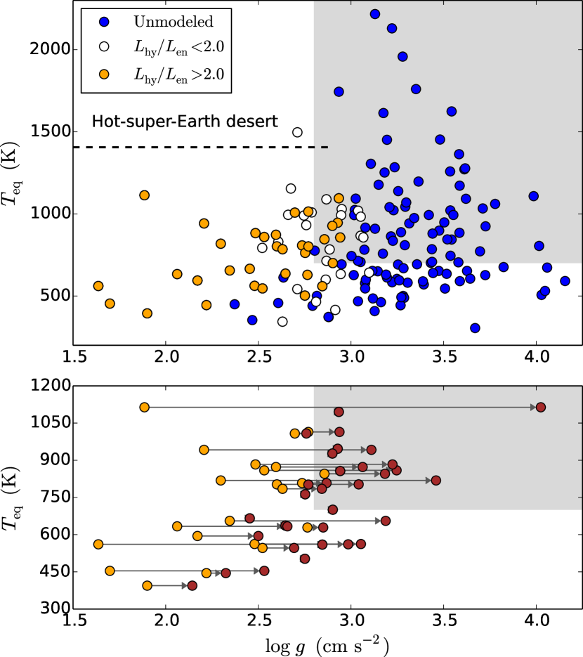
Figure 3: Planetary surface gravity vs. equilibrium-temperature. The orange, white, and blue circles (top panel) denote the extreme mass-loss rate, moderate mass-loss rate, and unmodeled planets, respectively. The gray and white background colors denote the region where planets have clear and cloudy-atmospheres, respectively, derived by Stevenson (2016) for hot Jupiters. The horizontal dashed line denotes the lowest incident-stellar-flux boundary (650 $F_{\oplus}$) of the hot-super-Earth desert (Lundkvist et al., 2016). The bottom panel shows the expected $\log g$ of the boil-off planets if their radii were corrected to have ${\Lambda}\equiv 20.0$ (brown circles) relative to their initial position (orange circles).

When we plot the planetary surface gravity, $\log g$, vs. equilibrium temperature for the planets in our sample (Fig. 3, top panel), we see that all boil-off planets are grouped in the $\log g<3.0$ region. While it is not surprising that these planets are concentrated at low $\log g$ values (given the similarity in mass and radius dependency of $\log g\propto M_{\rm p}\,R_{\rm p}^{-2}$ and ${\Lambda}\propto M_{\rm p}\,R_{\rm p}^{-1}$), it is interesting that this region limits closely to the boundary beweeen strong and weak J-band H₂O features observed in hot Jupiters, associated to cloudy vs. clear atmospheres, respectively (Stevenson, 2016). Regardless of whether there is a link between cloud processes on hot Jupiters and Neptune-like planets —two completely different samples—, this graph helps to identify planets with a higher prominence of clouds/hazes. Note that the derived surface gravity of these planets is also affected by the observational biases. Fig. 3 (bottom panel) shows the corrected $\log g$–$T$eq position of the boil-off planets if we assumed $R_{20}$ as the 100 mbar radius.

An important remark to highlight is that, while our analysis suggests that boil-off planets can have instead moderate mass-loss rates if they have cloudy atmospheres, we cannot claim that the remaining planets have clear atmospheres. They can either host clear or cloudy atmospheres. This occurs because our analysis is based on the dominant effect of hydrogen in the observed planetary radius. There can be cloudy planets with secondary atmospheres, or even hydrogen-dominated atmospheres hosting lower-altitude clouds that do not alter much the observed transit radius.

4.4 Bond-albedo Bias?

The cloudy-atmospheres scenario has a second consequence on the properties of these planets. The high-altitude cloud/haze layer would reflect a larger fraction of the incident stellar irradiation, decreasing the amount of energy deposited in the atmosphere, and consequently decreasing the estimated mass-loss rates. Low-density sub Neptunes (on average) would then differ from hot Jupiters. Studies of the aggregate sample of hot Jupiters show low geometric optical albedos ($A_{g}\approx 0.1$) and somewhat higher Bond albedos ($A_{B}=0.4\pm 0.1$, Schwartz & Cowan, 2015), suggesting that hot Jupiters have a layer of optical absorbers above an infra-red reflective cloud deck. Our cloudy-atmosphere case aligns well with the higher geometric albedos ($A_{g}\approx 0.16-0.3$) found on super-Earth planets ($R_{\rm p}<2.5{R_{\oplus}}$, Demory, 2014).

Table 1 shows the required values of the Bond albedo such that ${\Lambda}\equiv 20.0$ ($A_{20}$, keeping all other parameters fixed). Most of the planets in this list would require Bond albedos higher than any observed value from solar or extrasolar gas-giant planet.

If we confirm the cloudy nature of these atmospheres, this analysis places strong constraints on the atmospheric properties of the ensemble of low-density sub Neptunes. These planets would present high-altitude opaque clouds/hazes that increase the observed radii. Observationally, the value of their restricted Jeans escape parameter $\Lambda$, and also their position in the $\log g$–$T$eq plane, would be simple and direct indicators of the cloud/haze prominence on the atmospheres of these planets.

On a different but still interesting topic, the distribution of planets in the $\log g$–$T$eq plane (Fig. 3 top panel) agrees well with the proposed hot-super-Earth desert (Lundkvist et al., 2016). The boundary at 650 times the incident flux on Earth ($F_{\oplus}$) directly translates into an equilibrium temperature of $\sim 1400$ K. From the planets with known mass and radius, we observe a dearth of planets above this line. Unlike the $R_{\rm p}$–$F_{\oplus}$ figure from Lundkvist et al. (2016), this figure further constrains the parameter space of the planetary physical properties of the desert by adding information from the masses (through the surface gravity).

Furthermore, by considering the boil-off mass-loss regime, our results (Fig. 3 bottom panel) suggest that the exoplanet desert extends even further. Be it the mass or the radius of the planets being misinterpreted, boil-off planets should have a higher surface gravity, further depleting a region below the ${T_{\rm eq}}=1400$ K boundary, down to $\sim 600$ K.

5 CONCLUSIONS

We studied the mass-loss rates of the sample of 167 confirmed planets with masses $M_{\rm p}<30{M_{\oplus}}$. For 15% of the planets in this sample, we found that their planetary mass, radius, and equilibrium temperature lead to paradoxical results. Their observed low bulk densities imply hydrogen-dominated atmospheres. However, hydrodynamical models indicate extremely high mass-loss rates (${L_{\rm hy}}>0.1\ {M_{\oplus}}{\rm Gyr}^{-1}$), thus being unable to retain their hydrogen envelopes (boil-off regime).

Our hydrodynamical models’ mass-loss rates agree well with state-of-the-art models from the literature. Unfortunately, current observations do not offer a direct, model-independent validation of escape rates. Magnetic fields (however largely unknown) could offer a solution of this paradox by decreasing the predicted mass-loss rates (Owen & Adams, 2014; Khodachenko et al., 2015). Alternatively, the boil-off timescales of $\sim 10^{6}$ yr (Owen & Wu, 2016) could have been grossly underestimated. We need more detailed studies of the mass-loss time evolution during the boil-off regime.

If the model mass-loss estimations are correct, we hypothesize that either the TTV studies are underestimating the planetary masses or that these planets have high-altitude clouds/hazes producing overestimated transit radii, high albedos, or both. The cloudy/hazy scenario is further supported by the higher albedo found for super Earths, and a similar correlation as that between $\log g$–$T$eq and clear/cloudy atmospheres for hot Jupiters.

Whether we are misinterpreting their observed transit radii or underestimating their TTV masses, a fraction of $\sim$10–20% Neptunes with biased parameters will have a large impact on the population studies of the mass–radius relationship. Both empirical laws and physically motivated models tracing the observed mass-radius distribution of Neptunes would be disrupted by this sub-sample, simply because the observed values are not representative of the underlying properties of exoplanets. This could explain, for example, why studies like Wolfgang & Lopez (2015) do not find a direct mass–radius relationship for sub Neptune planets. In the future, population studies should consider the added complexity introduced by this rather large sub-sample of planets.

Conclusively solving this puzzle involves a multitude of studies, from the confirmation of low-densities with RV measurements, to the consistent modeling of high-altitude clouds/hazes. This study generates many open questions for the future, for example, can clouds/hazes form and remain at such high altitudes and under strong stellar irradiation conditions? Or how do reflective clouds affect the atmospheric albedo, and hence mass loss?

Appendix A PARAMETERS OF THE KNOWN NEPTUNE PLANETS

Table 2 list the observed and derived parameters for the known sample of Neptune-like planets.

Table 2: Observed and derived parameters for the sub-Neptune planet sample. This table only includes planets with estimated mass ($M_{\rm p}$) and transit radius ($R_{\rm p}$), with $M_{\rm p}<30{M_{\oplus}}$. The equilibrium temperature ($T$eq) assumes zero Bond albedo and efficient day–night energy redistribution. The restricted Jeans escape parameter ($\Lambda$) comes from Eq. (1). The planetary mean density ($\rho_{\rm p}$) assumes the observed mass and transit radius. $F_{\rm XUV}$ (section 3) is the stellar XUV-flux received by the planet for the given orbital semi-major axis ($a$), stellar mass ($M_{\rm s}$), age, and rotational angular velocity ($\Omega_{\rm rot}$). $L_{\rm hy}$ and $L_{\rm en}$ (section 3) are the hydrodynamic and energy-limited XUV-driven ($L_{\rm en}$) mass-loss rates of the selected hydrodynamic-modeled planets (mostly low-density planets with ${\Lambda}<20$).

Name	$M_{\rm p}$		$R_{\rm p}$		$T_{\rm eq}$	$\Lambda$	$\rho_{\rm p}$	$a$	$M_{\rm s}$	Age	$\Omega_{\rm rot}$	$F_{\rm XUV}$	$L_{\rm hy}$	$L_{\rm en}$	$L_{\rm hy}$/$L_{\rm en}$	Ref.a,b
	$M_{\oplus}$		$R_{\oplus}$		K		g cm-$3$	AU	$M_{\odot}$	Gyr	$\Omega_{\odot}$	erg s-$1$ cm-$2$	s-1	s-1
55 Cnc e	8.38	$\pm 0.39$	2.08	$\pm 0.16$	1957	15.6	5.14	0.015	0.91	10.2	1.4	173333.5	$\cdots$	$\cdots$	$\cdots$	De11R
CoRoT-22 b	12.08	${}_{-8.90}^{+13.99}$	4.88	${}_{-0.39}^{+0.17}$	1007	18.6	0.57	0.092	1.10	3.3	1.9	10959.0	3.4$\times$$10^{35}$	1.4$\times$$10^{35}$	2.3	Mou14R
CoRoT-24 c	27.97	$\pm 11.12$	4.94	$\pm 0.45$	706	60.8	1.28	0.098	0.91	11.0	1.3	2429.9	$\cdots$	$\cdots$	$\cdots$	Alo14R
CoRoT-7 b	5.72	$\pm 0.95$	1.58	$\pm 0.07$	1760	15.6	7.97	0.017	0.91	1.3	2.3	293392.3	$\cdots$	$\cdots$	$\cdots$	Ba14R
EPIC 2037 b	21.01	$\pm 5.40$	5.69	$\pm 0.56$	776	36.1	0.63	0.154	1.12	5.0	0.4	231.6	$\cdots$	$\cdots$	$\cdots$	Pet15R
EPIC 2037 c	27.00	$\pm 6.90$	7.83	$\pm 0.72$	612	42.7	0.31	0.247	1.12	5.0	0.4	90.0	$\cdots$	$\cdots$	$\cdots$	Pet15R
GJ 1132 b	1.62	$\pm 0.54$	1.16	$\pm 0.11$	578	18.4	5.79	0.015	0.18	5.0	5.2	156736.6	$\cdots$	$\cdots$	$\cdots$	BT15R
GJ 1214 b	6.36	$\pm 0.95$	2.28	$\pm 0.08$	599	35.3	2.97	0.014	0.18	6.0	5.2	181777.4	$\cdots$	$\cdots$	$\cdots$	Ha13R
GJ 3470 b	13.67	$\pm 1.59$	3.88	$\pm 0.33$	692	38.5	1.29	0.031	0.51	2.5	$\cdots$	5353.9	$\cdots$	$\cdots$	$\cdots$	Bi14R
GJ 436 b	22.25	$\pm 2.22$	4.17	$\pm 0.17$	642	62.9	1.69	0.029	0.47	6.0	0.3	699.6	1.3$\times$$10^{33}$	8.9$\times$$10^{33}$	0.1	Mac14R
HAT-P-11 b	25.75	$\pm 2.86$	4.74	$\pm 0.16$	866	47.6	1.34	0.053	0.81	6.5	1.1	5944.9	2.7$\times$$10^{34}$	2.4$\times$$10^{34}$	1.1	Bak10R
HAT-P-26 b	18.75	$\pm 2.22$	6.34	${}_{-0.36}^{+0.81}$	994	22.6	0.41	0.048	0.82	9.0	1.2	12237.8	4.4$\times$$10^{35}$	2.4$\times$$10^{35}$	1.8	Ha11R
HD 219134 b	4.46	$\pm 0.47$	1.61	$\pm 0.09$	1022	20.6	5.94	0.038	0.79	12.5	0.3	926.6	$\cdots$	$\cdots$	$\cdots$	Mot15R
HD 97658 b	7.63	${}_{-0.64}^{+0.95}$	2.24	${}_{-0.09}^{+0.10}$	758	34.0	3.72	0.080	0.77	6.0	0.4	485.1	$\cdots$	$\cdots$	$\cdots$	VG14R
HIP 116454 b	11.76	$\pm 1.27$	2.54	$\pm 0.18$	691	50.8	3.98	0.091	0.78	2.0	1.5	4879.7	$\cdots$	$\cdots$	$\cdots$	V15R
K2-19 c	15.90	${}_{-2.80}^{+7.70}$	4.51	$\pm 0.47$	783	34.1	0.96	0.100	0.95	$\cdots$	0.5	540.3	6.4$\times$$10^{33}$	3.2$\times$$10^{33}$	2.0	Ba15R,T
K2-3 b	8.40	$\pm 2.10$	2.08	${}_{-0.09}^{+0.18}$	500	61.3	5.18	0.077	0.61	2.0	$\cdots$	1232.2	$\cdots$	$\cdots$	$\cdots$	Alm15R
K2-3 c	2.10	${}_{-1.30}^{+2.10}$	1.65	${}_{-0.07}^{+0.16}$	371	26.0	2.58	0.141	0.61	2.0	$\cdots$	374.9	$\cdots$	$\cdots$	$\cdots$	Alm15R
K2-3 d	11.10	$\pm 3.50$	1.53	$\pm 0.11$	305	180.8	17.22	0.209	0.61	2.0	$\cdots$	170.1	$\cdots$	$\cdots$	$\cdots$	Alm15R
K2-56 b	16.30	${}_{-6.10}^{+6.00}$	2.23	${}_{-0.11}^{+0.14}$	545	101.6	8.11	0.241	0.96	3.3	1.9	1517.7	$\cdots$	$\cdots$	$\cdots$	E16R
Kepler-10 b	3.72	$\pm 0.42$	1.48	${}_{-0.03}^{+0.04}$	2129	8.9	6.31	0.017	0.91	9.1	1.0	124224.8	$\cdots$	$\cdots$	$\cdots$	W16R
Kepler-10 c	13.98	$\pm 1.79$	2.36	${}_{-0.04}^{+0.09}$	570	78.8	5.89	0.240	0.91	9.1	1.0	639.6	$\cdots$	$\cdots$	$\cdots$	W16R
Kepler-100 b	7.31	$\pm 3.18$	1.32	$\pm 0.04$	1271	32.9	17.37	0.073	1.08	6.9	1.3	14282.2	$\cdots$	$\cdots$	$\cdots$	Mar14R
Kepler-102 d	3.81	$\pm 1.91$	1.18	$\pm 0.04$	701	35.0	12.86	0.086	0.81	4.1	0.4	302.8	$\cdots$	$\cdots$	$\cdots$	Mar14R
Kepler-102 e	8.90	$\pm 1.91$	2.22	$\pm 0.07$	604	50.3	4.47	0.117	0.81	4.1	0.4	166.5	$\cdots$	$\cdots$	$\cdots$	Mar14R
Kepler-103 b	9.85	$\pm 8.58$	3.38	$\pm 0.09$	946	23.4	1.41	0.128	1.09	6.0	0.9	2165.8	3.1$\times$$10^{34}$	9.0$\times$$10^{33}$	3.4	Mar14R
Kepler-104 b	19.60	${}_{-12.40}^{+14.50}$	3.13	${}_{-0.70}^{+0.52}$	1043	45.5	3.53	0.094	0.81	3.7	$\cdots$	5720.3	$\cdots$	$\cdots$	$\cdots$	HL14T
Kepler-105 b	3.70	$\pm 2.00$	2.22	$\pm 0.11$	1088	11.6	1.87	0.060	0.96	3.5	1.6	17615.2	3.8$\times$$10^{35}$	2.1$\times$$10^{35}$	1.8	JH15bT
Kepler-105 c	4.60	$\pm 0.90$	1.31	$\pm 0.07$	993	26.8	11.28	0.072	0.96	3.5	1.6	12198.6	$\cdots$	$\cdots$	$\cdots$	JH15bT
Kepler-106 c	10.49	$\pm 3.18$	2.50	$\pm 0.33$	863	36.8	3.69	0.111	1.00	3.3	0.2	68.5	$\cdots$	$\cdots$	$\cdots$	Mar14R
Kepler-106 e	11.12	$\pm 5.72$	2.56	$\pm 0.33$	583	56.5	3.66	0.243	1.00	3.3	0.2	14.3	$\cdots$	$\cdots$	$\cdots$	Mar14R
Kepler-11 b	1.91	${}_{-0.95}^{+1.27}$	1.81	${}_{-0.04}^{+0.03}$	931	8.6	1.78	0.091	0.96	6.9	0.2	175.8	2.2$\times$$10^{35}$	8.7$\times$$10^{33}$	25.3	L13T
Kepler-11 c	2.86	${}_{-1.59}^{+2.86}$	2.87	${}_{-0.06}^{+0.04}$	859	8.8	0.67	0.107	0.96	6.9	0.2	127.2	4.0$\times$$10^{35}$	1.5$\times$$10^{34}$	26.7	L13T
Kepler-11 d	7.31	${}_{-1.59}^{+0.95}$	3.12	${}_{-0.07}^{+0.06}$	714	24.9	1.33	0.155	0.96	6.9	0.2	60.6	3.6$\times$$10^{32}$	3.5$\times$$10^{32}$	1.0	L13T
Kepler-11 e	7.95	${}_{-2.22}^{+1.59}$	4.20	${}_{-0.09}^{+0.07}$	636	22.6	0.59	0.195	0.96	6.9	0.2	38.3	2.0$\times$$10^{33}$	4.9$\times$$10^{32}$	4.1	L13T
Kepler-11 f	1.91	$\pm 0.95$	2.49	${}_{-0.07}^{+0.04}$	562	10.3	0.68	0.250	0.96	6.9	0.2	23.3	8.4$\times$$10^{34}$	2.8$\times$$10^{33}$	30.0	L13T
Kepler-113 b	11.76	$\pm 4.13$	1.82	$\pm 0.04$	844	58.1	10.80	0.050	0.75	3.2	0.3	635.2	$\cdots$	$\cdots$	$\cdots$	Mar14R
Kepler-114 c	2.86	$\pm 0.64$	1.60	$\pm 0.18$	714	18.9	3.82	0.065	0.56	2.7	0.9	4657.9	$\cdots$	$\cdots$	$\cdots$	X14T
Kepler-114 d	3.81	$\pm 1.59$	2.54	$\pm 0.28$	628	18.1	1.29	0.083	0.56	2.7	0.9	2796.6	6.1$\times$$10^{34}$	1.8$\times$$10^{34}$	3.4	X14T
Kepler-120 b	8.50	${}_{-7.50}^{+9.70}$	2.31	$\pm 0.37$	613	45.5	3.80	0.055	0.59	3.6	$\cdots$	1524.5	$\cdots$	$\cdots$	$\cdots$	HL14T
Kepler-122 e	27.70	${}_{-9.80}^{+11.40}$	2.02	${}_{-0.19}^{+0.70}$	676	153.8	18.53	0.227	0.99	3.9	$\cdots$	1104.9	$\cdots$	$\cdots$	$\cdots$	HL14T
Kepler-131 b	16.21	$\pm 3.50$	2.41	$\pm 0.20$	785	64.9	6.37	0.126	1.02	3.7	0.2	79.2	$\cdots$	$\cdots$	$\cdots$	Mar14R
Kepler-131 c	8.26	$\pm 6.04$	0.84	$\pm 0.07$	673	110.6	76.46	0.171	1.02	3.7	0.2	42.9	$\cdots$	$\cdots$	$\cdots$	Mar14R
Kepler-136 b	19.80	${}_{-10.40}^{+11.70}$	1.80	${}_{-0.17}^{+0.35}$	1060	78.6	18.72	0.106	1.20	2.8	$\cdots$	12210.7	$\cdots$	$\cdots$	$\cdots$	HL14T
Kepler-138 b	0.07	${}_{-0.04}^{+0.06}$	0.53	$\pm 0.03$	449	2.1	2.51	0.075	0.52	4.7	1.4	2705.8	$\cdots$	$\cdots$	$\cdots$	JH15aT
Kepler-138 c	1.97	${}_{-1.12}^{+1.91}$	1.20	$\pm 0.07$	408	30.5	6.28	0.090	0.52	4.7	1.4	1838.5	$\cdots$	$\cdots$	$\cdots$	JH15aT
Kepler-138 d	0.64	${}_{-0.39}^{+0.67}$	1.21	$\pm 0.08$	343	11.6	1.98	0.128	0.52	4.7	1.4	924.8	8.4$\times$$10^{34}$	1.2$\times$$10^{34}$	7.1	JH15aT

Table 3: continued

Sub-Neptune Planet Parameters. Name $M_{\rm p}$ $R_{\rm p}$ $T_{\rm eq}$ $\Lambda$ $\rho_{\rm p}$ $a$ $M_{\rm s}$ Age $\Omega_{\rm rot}$ $F_{\rm XUV}$ $L_{\rm hy}$ $L_{\rm en}$ $L_{\rm hy}$/$L_{\rm en}$ Ref.^a,b $M_{\oplus}$ $R_{\oplus}$ K g cm^-3 AU $M_{\odot}$ Gyr $\Omega_{\odot}$ erg s-$1$ cm-$2$ s^-1 s^-1 Kepler-161 b 12.10 ${}_{-6.30}^{+7.40}$ 1.93 ${}_{-0.14}^{+0.31}$ 948 50.1 9.28 0.054 0.77 4.7 1.0 7681.3 $\cdots$ $\cdots$ $\cdots$ HL14^T Kepler-161 c 11.80 ${}_{-7.50}^{+10.50}$ 1.87 ${}_{-0.14}^{+0.30}$ 844 56.6 9.95 0.068 0.77 4.7 1.0 4844.0 $\cdots$ $\cdots$ $\cdots$ HL14^T Kepler-176 c 23.00 ${}_{-8.00}^{+13.50}$ 2.56 ${}_{-0.26}^{+0.93}$ 745 91.4 7.56 0.102 0.83 4.7 0.8 1567.5 $\cdots$ $\cdots$ $\cdots$ HL14^T Kepler-176 d 15.20 ${}_{-5.80}^{+10.40}$ 2.47 ${}_{-0.25}^{+0.90}$ 589 79.2 5.56 0.163 0.83 4.7 0.8 613.8 $\cdots$ $\cdots$ $\cdots$ HL14^T Kepler-177 b 1.91 ${}_{-0.32}^{+0.64}$ 2.91 ${}_{-0.30}^{+1.53}$ 655 7.6 0.43 0.222 1.07 4.4 $\cdots$ 962.8 4.1$\times$$10^{36}$ 2.0$\times$$10^{35}$ 20.5 X14^T Kepler-177 c 7.63 ${}_{-3.18}^{+3.50}$ 7.10 ${}_{-0.72}^{+3.71}$ 594 13.7 0.12 0.270 1.07 4.4 $\cdots$ 651.5 5.8$\times$$10^{35}$ 1.0$\times$$10^{35}$ 5.8 X14^T Kepler-18 b 6.99 $\pm 3.50$ 2.00 $\pm 0.10$ 1284 20.7 4.84 0.045 0.97 10.7 1.9 46258.8 $\cdots$ $\cdots$ $\cdots$ Co11^R,T Kepler-18 c 17.16 $\pm 1.91$ 5.50 $\pm 0.26$ 990 23.9 0.57 0.075 0.97 10.7 1.9 16344.6 3.3$\times$$10^{35}$ 2.1$\times$$10^{35}$ 1.6 Co11^R,T Kepler-18 d 16.53 $\pm 1.27$ 6.99 $\pm 0.33$ 793 22.6 0.27 0.117 0.97 10.7 1.9 6729.1 3.5$\times$$10^{35}$ 1.9$\times$$10^{35}$ 1.8 Co11^R,T Kepler-184 c 8.80 ${}_{-5.70}^{+7.40}$ 1.95 ${}_{-0.19}^{+0.84}$ 693 49.4 6.55 0.141 0.87 4.5 $\cdots$ 1017.7 $\cdots$ $\cdots$ $\cdots$ HL14^T Kepler-189 c 22.70 ${}_{-10.60}^{+17.10}$ 2.40 ${}_{-0.18}^{+0.52}$ 590 121.5 9.06 0.137 0.84 5.2 $\cdots$ 497.7 $\cdots$ $\cdots$ $\cdots$ HL14^T Kepler-197 c 5.30 ${}_{-2.90}^{+3.30}$ 1.23 $\pm 0.04$ 1021 32.0 15.71 0.090 0.92 5.4 $\cdots$ 3777.0 $\cdots$ $\cdots$ $\cdots$ HL14^T Kepler-20 b 8.58 $\pm 2.22$ 1.91 ${}_{-0.21}^{+0.12}$ 1197 28.5 6.82 0.045 0.91 5.2 0.2 732.8 $\cdots$ $\cdots$ $\cdots$ Ga12^R Kepler-20 c 16.21 ${}_{-3.81}^{+3.18}$ 3.07 ${}_{-0.31}^{+0.20}$ 836 47.8 3.08 0.093 0.91 5.2 0.2 174.6 $\cdots$ $\cdots$ $\cdots$ Ga12^R Kepler-211 c 18.30 ${}_{-17.00}^{+22.40}$ 2.45 ${}_{-1.09}^{+1.62}$ 898 63.1 6.86 0.062 0.97 1.6 2.0 12588.9 $\cdots$ $\cdots$ $\cdots$ HL14^T Kepler-215 d 23.60 ${}_{-11.90}^{+17.30}$ 2.34 ${}_{-0.34}^{+0.44}$ 652 117.1 10.16 0.185 0.77 1.6 $\cdots$ 2352.6 $\cdots$ $\cdots$ $\cdots$ HL14^T Kepler-219 d 19.10 ${}_{-17.70}^{+29.90}$ 2.51 ${}_{-0.40}^{+0.63}$ 652 88.4 6.66 0.272 1.15 4.6 1.6 1158.9 $\cdots$ $\cdots$ $\cdots$ HL14^T Kepler-221 c 15.10 ${}_{-6.70}^{+10.10}$ 2.68 ${}_{-0.26}^{+0.61}$ 942 45.3 4.33 0.059 0.72 4.6 2.9 70313.6 $\cdots$ $\cdots$ $\cdots$ HL14^T Kepler-226 b 24.00 ${}_{-10.10}^{+11.80}$ 1.56 ${}_{-0.12}^{+0.58}$ 1108 105.3 34.86 0.047 0.86 4.4 $\cdots$ 7076.1 $\cdots$ $\cdots$ $\cdots$ HL14^T Kepler-23 b 15.20 ${}_{-2.90}^{+3.20}$ 1.90 $\pm 0.06$ 1277 47.5 12.22 0.075 1.11 6.6 $\cdots$ 8385.5 $\cdots$ $\cdots$ $\cdots$ HL14^T Kepler-23 d 17.60 ${}_{-11.90}^{+13.70}$ 2.20 $\pm 0.07$ 993 61.1 9.12 0.124 1.11 6.6 $\cdots$ 3067.7 $\cdots$ $\cdots$ $\cdots$ HL14^T Kepler-231 b 4.90 ${}_{-1.30}^{+1.80}$ 1.82 ${}_{-0.25}^{+0.26}$ 462 44.1 4.48 0.074 0.51 3.5 1.2 2185.7 $\cdots$ $\cdots$ $\cdots$ K14^T Kepler-231 c 2.20 ${}_{-1.10}^{+1.50}$ 1.69 ${}_{-0.23}^{+0.24}$ 372 26.5 2.51 0.114 0.51 3.5 1.2 921.0 $\cdots$ $\cdots$ $\cdots$ K14^T Kepler-238 f 13.35 ${}_{-2.54}^{+2.86}$ 2.00 ${}_{-0.17}^{+0.85}$ 635 79.8 9.24 0.272 1.06 6.8 $\cdots$ 507.0 $\cdots$ $\cdots$ $\cdots$ X14^T Kepler-244 d 15.20 ${}_{-13.00}^{+20.00}$ 2.32 ${}_{-0.18}^{+0.83}$ 640 77.6 6.71 0.140 0.88 4.8 $\cdots$ 720.1 $\cdots$ $\cdots$ $\cdots$ HL14^T Kepler-245 d 21.60 ${}_{-12.10}^{+16.60}$ 3.31 ${}_{-0.37}^{+1.40}$ 489 101.1 3.28 0.202 0.80 3.6 1.4 987.3 $\cdots$ $\cdots$ $\cdots$ HL14^T Kepler-25 b 9.60 $\pm 4.20$ 2.71 $\pm 0.05$ 1305 20.6 2.65 0.070 1.19 2.9 3.9 92614.7 $\cdots$ $\cdots$ $\cdots$ Mar14^R Kepler-25 c 24.60 $\pm 5.70$ 5.21 $\pm 0.09$ 1029 34.8 0.96 0.113 1.19 2.9 3.9 35845.4 1.6$\times$$10^{35}$ 1.7$\times$$10^{35}$ 0.9 Mar14^R Kepler-254 c 3.20 ${}_{-2.70}^{+3.70}$ 2.09 ${}_{-0.16}^{+0.84}$ 845 13.7 1.93 0.105 0.97 4.0 1.1 2984.8 9.1$\times$$10^{34}$ 2.9$\times$$10^{34}$ 3.1 HL14^T Kepler-26 b 5.10 $\pm 0.70$ 2.78 $\pm 0.11$ 465 29.9 1.31 0.085 0.54 3.0 2.0 5260.6 2.7$\times$$10^{34}$ 2.8$\times$$10^{34}$ 1.0 JH15b^T Kepler-26 c 6.20 $\pm 0.70$ 2.72 $\pm 0.12$ 415 41.6 1.70 0.107 0.54 3.0 2.0 3338.5 5.8$\times$$10^{33}$ 1.7$\times$$10^{34}$ 0.3 JH15b^T Kepler-27 c 21.20 ${}_{-3.70}^{+3.20}$ 7.17 ${}_{-0.27}^{+0.38}$ 457 49.0 0.32 0.191 0.65 1.6 0.5 222.8 $\cdots$ $\cdots$ $\cdots$ HL14^T Kepler-276 c 16.53 ${}_{-3.50}^{+4.45}$ 2.91 ${}_{-0.28}^{+1.27}$ 669 64.4 3.71 0.203 1.10 3.8 $\cdots$ 1237.2 $\cdots$ $\cdots$ $\cdots$ X14^T Kepler-276 d 16.21 ${}_{-4.45}^{+5.09}$ 2.81 ${}_{-0.27}^{+1.23}$ 581 75.4 4.05 0.269 1.10 3.8 $\cdots$ 704.2 $\cdots$ $\cdots$ $\cdots$ X14^T Kepler-28 b 8.80 ${}_{-3.10}^{+3.80}$ 2.93 $\pm 0.46$ 743 30.6 1.93 0.062 0.75 2.2 1.5 7830.8 $\cdots$ $\cdots$ $\cdots$ HL14^T Kepler-28 c 10.90 ${}_{-4.50}^{+6.10}$ 2.77 $\pm 0.44$ 650 45.9 2.83 0.081 0.75 2.2 1.5 4587.9 $\cdots$ $\cdots$ $\cdots$ HL14^T Kepler-289 b 7.31 $\pm 6.67$ 2.15 $\pm 0.10$ 630 40.8 4.03 0.210 1.08 3.8 3.0 4490.4 $\cdots$ $\cdots$ $\cdots$ S14^T Kepler-289 d 4.13 $\pm 0.95$ 2.68 $\pm 0.17$ 502 23.2 1.18 0.330 1.08 3.8 3.0 1818.4 4.1$\times$$10^{34}$ 1.9$\times$$10^{34}$ 2.2 S14^T Kepler-29 b 4.50 $\pm 1.50$ 3.35 $\pm 0.22$ 872 11.7 0.66 0.092 0.98 $\cdots$ 2.3 13666.1 1.3$\times$$10^{36}$ 4.0$\times$$10^{35}$ 3.3 JH15b^T Kepler-29 c 4.00 $\pm 1.30$ 3.14 $\pm 0.20$ 802 12.0 0.71 0.109 0.98 $\cdots$ 2.3 9778.1 8.9$\times$$10^{35}$ 2.8$\times$$10^{35}$ 3.2 JH15b^T Kepler-30 b 11.30 $\pm 1.40$ 3.90 $\pm 0.20$ 599 36.7 1.05 0.186 0.99 1.6 1.1 718.8 7.5$\times$$10^{33}$ 4.3$\times$$10^{33}$ 1.7 SO12^T Kepler-30 d 23.10 $\pm 2.70$ 8.79 $\pm 0.50$ 353 56.4 0.19 0.534 0.99 1.6 1.1 86.7 $\cdots$ $\cdots$ $\cdots$ SO12^T Kepler-305 b 10.49 ${}_{-1.91}^{+2.54}$ 3.60 ${}_{-0.36}^{+0.90}$ 927 23.8 1.24 0.056 0.76 4.4 $\cdots$ 3742.0 5.1$\times$$10^{34}$ 2.4$\times$$10^{34}$ 2.1 X14^T Kepler-305 c 6.04 ${}_{-2.22}^{+2.54}$ 3.30 ${}_{-0.33}^{+0.82}$ 808 17.2 0.93 0.073 0.76 4.4 $\cdots$ 2158.9 8.0$\times$$10^{34}$ 2.5$\times$$10^{34}$ 3.2 X14^T Kepler-307 b 3.18 $\pm 0.64$ 3.20 ${}_{-0.46}^{+1.20}$ 883 8.5 0.54 0.093 0.98 6.6 2.0 11054.6 3.9$\times$$10^{36}$ 9.5$\times$$10^{35}$ 4.1 X14^T Kepler-307 c 1.59 ${}_{-0.32}^{+0.64}$ 2.81 ${}_{-0.42}^{+1.05}$ 818 5.2 0.40 0.108 0.98 6.6 2.0 8159.4 9.8$\times$$10^{37}$ 1.2$\times$$10^{36}$ 81.7 X14^T Kepler-31 c 29.50 ${}_{-7.00}^{+9.60}$ 4.71 ${}_{-0.57}^{+2.23}$ 653 72.7 1.56 0.260 1.21 4.2 $\cdots$ 1108.1 $\cdots$ $\cdots$ $\cdots$ HL14^T Kepler-32 b 9.40 ${}_{-3.10}^{+3.60}$ 2.25 $\pm 0.11$ 595 53.2 4.55 0.050 0.54 2.7 0.8 2232.3 $\cdots$ $\cdots$ $\cdots$ HL14^T Kepler-32 c 7.70 ${}_{-3.80}^{+5.00}$ 2.02 $\pm 0.11$ 443 65.1 5.15 0.090 0.54 2.7 0.8 689.0 $\cdots$ $\cdots$ $\cdots$ HL14^T Kepler-326 c 17.40 ${}_{-10.70}^{+15.40}$ 2.79 ${}_{-1.31}^{+1.96}$ 974 48.5 4.42 0.051 0.98 4.7 2.8 34240.8 $\cdots$ $\cdots$ $\cdots$ HL14^T Kepler-326 d 6.90 ${}_{-5.90}^{+8.50}$ 2.41 ${}_{-1.13}^{+1.70}$ 856 25.3 2.72 0.066 0.98 4.7 2.8 20445.5 4.7$\times$$10^{34}$ 6.1$\times$$10^{34}$ 0.8 HL14^T

Table 4: continued

Sub-Neptune Planet Parameters. Name $M_{\rm p}$ $R_{\rm p}$ $T_{\rm eq}$ $\Lambda$ $\rho_{\rm p}$ $a$ $M_{\rm s}$ Age $\Omega_{\rm rot}$ $F_{\rm XUV}$ $L_{\rm hy}$ $L_{\rm en}$ $L_{\rm hy}$/$L_{\rm en}$ Ref.^a,b $M_{\oplus}$ $R_{\oplus}$ K g cm^-3 AU $M_{\odot}$ Gyr $\Omega_{\odot}$ erg s-$1$ cm-$2$ s^-1 s^-1 Kepler-327 c 20.30 ${}_{-17.70}^{+27.10}$ 1.18 $\pm 0.11$ 591 220.6 68.14 0.047 0.55 3.0 1.1 4264.3 $\cdots$ $\cdots$ $\cdots$ HL14^T Kepler-328 b 28.61 ${}_{-12.40}^{+13.03}$ 2.30 ${}_{-0.24}^{+0.97}$ 627 150.3 12.96 0.219 1.15 2.6 $\cdots$ 1487.0 $\cdots$ $\cdots$ $\cdots$ X14^T Kepler-33 c 0.80 ${}_{-0.70}^{+2.50}$ 3.20 $\pm 0.30$ 1113 1.7 0.13 0.119 1.29 4.4 1.0 2707.6 2.2$\times$$10^{42}$ 1.4$\times$$10^{36}$ 1.6$\times$$10^{6}$ HL16^T Kepler-33 d 4.70 $\pm 2.00$ 5.35 $\pm 0.49$ 941 7.1 0.17 0.166 1.29 4.4 1.0 1385.8 1.8$\times$$10^{37}$ 7.5$\times$$10^{35}$ 24.0 HL16^T Kepler-33 e 6.70 ${}_{-1.30}^{+1.20}$ 4.03 $\pm 0.38$ 830 15.2 0.57 0.214 1.29 4.4 1.0 837.4 3.3$\times$$10^{34}$ 2.8$\times$$10^{34}$ 1.2 HL16^T Kepler-33 f 11.50 ${}_{-2.10}^{+1.80}$ 4.47 $\pm 0.42$ 762 25.6 0.71 0.254 1.29 4.4 1.0 595.6 1.8$\times$$10^{34}$ 6.1$\times$$10^{33}$ 3.0 HL16^T Kepler-333 b 28.20 ${}_{-24.10}^{+29.00}$ 1.61 $\pm 0.17$ 506 262.1 37.27 0.087 0.54 3.2 1.1 2381.1 $\cdots$ $\cdots$ $\cdots$ HL14^T Kepler-338 e 8.50 ${}_{-6.30}^{+7.20}$ 1.56 $\pm 0.07$ 1258 32.8 12.35 0.090 1.10 4.8 $\cdots$ 10799.4 $\cdots$ $\cdots$ $\cdots$ HL14^T Kepler-339 c 7.30 ${}_{-6.20}^{+7.80}$ 1.16 ${}_{-0.09}^{+0.45}$ 924 51.6 25.79 0.069 0.84 4.4 1.6 13691.2 $\cdots$ $\cdots$ $\cdots$ HL14^T Kepler-339 d 14.70 ${}_{-10.00}^{+14.10}$ 1.18 ${}_{-0.09}^{+0.46}$ 804 117.4 49.34 0.091 0.84 4.4 1.6 7871.5 $\cdots$ $\cdots$ $\cdots$ HL14^T Kepler-350 c 6.04 $\pm 3.18$ 3.11 ${}_{-0.61}^{+1.43}$ 1009 14.6 1.11 0.134 1.00 3.2 8.5 243252.4 1.6$\times$$10^{36}$ 1.8$\times$$10^{36}$ 0.9 X14^T Kepler-350 d 14.94 ${}_{-4.77}^{+5.40}$ 2.81 ${}_{-0.54}^{+1.28}$ 888 45.4 3.73 0.172 1.00 3.2 8.5 146470.2 $\cdots$ $\cdots$ $\cdots$ X14^T Kepler-351 b 4.80 ${}_{-4.70}^{+5.70}$ 3.03 ${}_{-0.24}^{+1.33}$ 542 22.2 0.95 0.214 0.89 4.9 $\cdots$ 356.0 5.6$\times$$10^{33}$ 3.6$\times$$10^{33}$ 1.6 HL14^T Kepler-351 c 11.10 ${}_{-7.60}^{+9.90}$ 3.16 ${}_{-0.25}^{+1.38}$ 468 56.9 1.94 0.287 0.89 4.9 $\cdots$ 197.9 $\cdots$ $\cdots$ $\cdots$ HL14^T Kepler-36 b 4.46 ${}_{-0.27}^{+0.33}$ 1.48 $\pm 0.03$ 1069 21.3 7.52 0.115 1.07 4.8 1.6 10334.7 $\cdots$ $\cdots$ $\cdots$ Ca12^T Kepler-36 c 8.10 ${}_{-0.46}^{+0.60}$ 3.68 $\pm 0.05$ 1014 16.5 0.90 0.128 1.07 4.8 1.6 8348.0 2.5$\times$$10^{35}$ 1.2$\times$$10^{35}$ 2.1 Ca12^T Kepler-385 b 12.80 ${}_{-6.80}^{+11.40}$ 2.79 ${}_{-0.35}^{+1.62}$ 1041 33.4 3.25 0.097 1.09 3.3 $\cdots$ 8110.4 $\cdots$ $\cdots$ $\cdots$ HL14^T Kepler-385 c 13.20 ${}_{-9.00}^{+16.80}$ 3.10 ${}_{-0.39}^{+1.81}$ 909 35.5 2.44 0.127 1.09 3.3 $\cdots$ 4731.3 $\cdots$ $\cdots$ $\cdots$ HL14^T Kepler-396 c 17.80 ${}_{-1.27}^{+2.86}$ 5.31 ${}_{-0.99}^{+1.95}$ 440 57.7 0.66 0.368 0.85 4.4 2.0 1032.9 $\cdots$ $\cdots$ $\cdots$ X14^T Kepler-4 b 24.47 $\pm 3.81$ 4.01 $\pm 0.21$ 1614 28.7 2.10 0.046 1.22 6.8 0.8 9535.9 $\cdots$ $\cdots$ $\cdots$ Bo10^R Kepler-406 b 6.36 $\pm 1.27$ 1.44 $\pm 0.03$ 1452 23.1 11.83 0.036 1.07 2.1 0.2 758.8 $\cdots$ $\cdots$ $\cdots$ Mar14^R Kepler-406 c 2.86 $\pm 1.91$ 0.85 $\pm 0.03$ 1171 21.7 25.43 0.056 1.07 2.1 0.2 321.0 $\cdots$ $\cdots$ $\cdots$ Mar14^R Kepler-454 b 6.84 $\pm 1.40$ 2.37 $\pm 0.13$ 916 23.9 2.83 0.095 1.03 4.3 1.2 4051.6 $\cdots$ $\cdots$ $\cdots$ Ge15^R Kepler-48 b 3.94 $\pm 2.10$ 1.92 $\pm 0.10$ 1024 15.2 3.07 0.053 0.88 6.2 0.3 759.5 $\cdots$ $\cdots$ $\cdots$ Mar14^R Kepler-48 c 14.61 $\pm 2.30$ 2.71 $\pm 0.14$ 809 50.5 4.05 0.085 0.88 6.2 0.3 296.8 $\cdots$ $\cdots$ $\cdots$ Mar14^R Kepler-48 d 7.95 $\pm 4.61$ 2.04 $\pm 0.11$ 492 59.9 5.14 0.230 0.88 6.2 0.3 40.7 $\cdots$ $\cdots$ $\cdots$ Mar14^R Kepler-49 b 7.80 ${}_{-3.90}^{+15.40}$ 2.72 $\pm 0.12$ 627 34.7 2.14 0.060 0.55 2.9 1.5 8833.6 $\cdots$ $\cdots$ $\cdots$ X13^T Kepler-49 c 7.90 ${}_{-3.90}^{+15.60}$ 2.55 $\pm 0.13$ 546 43.0 2.63 0.079 0.55 2.9 1.5 5074.4 $\cdots$ $\cdots$ $\cdots$ X13^T Kepler-51 b 2.22 ${}_{-0.95}^{+1.59}$ 7.10 $\pm 0.30$ 561 4.2 0.03 0.251 1.04 3.4 3.3 3724.8 1.8$\times$$10^{39}$ 1.0$\times$$10^{37}$ 180.0 Mas14^T Kepler-51 c 4.13 $\pm 0.32$ 9.01 ${}_{-1.71}^{+2.81}$ 453 7.7 0.03 0.384 1.04 3.4 3.3 1596.5 5.3$\times$$10^{37}$ 4.5$\times$$10^{36}$ 11.8 Mas14^T Kepler-51 d 7.63 $\pm 0.95$ 9.71 $\pm 0.50$ 394 15.1 0.05 0.509 1.04 3.4 3.3 908.7 1.3$\times$$10^{36}$ 3.8$\times$$10^{35}$ 3.4 Mas14^T Kepler-54 b 21.50 ${}_{-4.90}^{+5.60}$ 2.19 $\pm 0.07$ 605 122.9 11.29 0.063 0.51 4.2 0.8 2727.7 $\cdots$ $\cdots$ $\cdots$ HL14^T Kepler-54 c 19.80 ${}_{-4.40}^{+6.60}$ 1.32 $\pm 0.08$ 530 214.3 47.48 0.082 0.51 4.2 0.8 1610.1 $\cdots$ $\cdots$ $\cdots$ HL14^T Kepler-56 b 22.25 ${}_{-3.50}^{+3.81}$ 6.52 ${}_{-0.28}^{+0.29}$ 1496 17.3 0.44 0.103 1.32 4.4 $\cdots$ 18720.8 7.8$\times$$10^{35}$ 4.2$\times$$10^{35}$ 1.9 H13^T Kepler-57 c 9.30 ${}_{-3.00}^{+25.20}$ 1.55 $\pm 0.67$ 705 64.5 13.77 0.092 0.76 4.7 0.8 1761.3 $\cdots$ $\cdots$ $\cdots$ X13^T Kepler-60 b 4.20 $\pm 0.60$ 1.71 $\pm 0.13$ 1177 15.8 4.63 0.073 1.04 5.1 $\cdots$ 8080.2 $\cdots$ $\cdots$ $\cdots$ JH15b^T Kepler-60 c 3.90 $\pm 0.80$ 1.90 $\pm 0.15$ 1092 14.2 3.14 0.085 1.04 5.1 $\cdots$ 5999.3 $\cdots$ $\cdots$ $\cdots$ JH15b^T Kepler-60 d 4.20 $\pm 0.80$ 1.99 $\pm 0.16$ 992 16.1 2.94 0.103 1.04 5.1 $\cdots$ 4082.8 $\cdots$ $\cdots$ $\cdots$ JH15b^T Kepler-65 c 26.60 ${}_{-18.50}^{+20.40}$ 2.61 $\pm 0.04$ 1363 56.7 8.25 0.068 1.25 3.3 4.0 96951.2 $\cdots$ $\cdots$ $\cdots$ HL14^T Kepler-68 b 8.26 ${}_{-2.54}^{+2.22}$ 2.31 ${}_{-0.09}^{+0.06}$ 1252 21.7 3.69 0.062 1.08 6.3 0.2 441.3 $\cdots$ $\cdots$ $\cdots$ Gi13^R Kepler-68 c 4.77 ${}_{-3.50}^{+2.54}$ 0.95 ${}_{-0.04}^{+0.03}$ 1033 36.7 30.30 0.091 1.08 6.3 0.2 204.7 $\cdots$ $\cdots$ $\cdots$ Gi13^R Kepler-78 b 1.91 $\pm 0.32$ 1.18 ${}_{-0.09}^{+0.16}$ 2217 5.5 6.43 0.009 0.76 0.8 1.7 731021.4 $\cdots$ $\cdots$ $\cdots$ Pep13^R Kepler-79 b 10.90 ${}_{-6.04}^{+7.31}$ 3.48 $\pm 0.07$ 992 24.0 1.43 0.117 1.17 3.2 $\cdots$ 6920.5 7.6$\times$$10^{34}$ 6.3$\times$$10^{34}$ 1.2 JH14^T Kepler-79 c 6.04 ${}_{-2.29}^{+1.91}$ 3.73 $\pm 0.08$ 784 15.7 0.64 0.187 1.17 3.2 $\cdots$ 2709.1 1.7$\times$$10^{35}$ 7.4$\times$$10^{34}$ 2.3 JH14^T Kepler-79 d 6.04 ${}_{-1.59}^{+2.10}$ 7.17 ${}_{-0.16}^{+0.13}$ 633 10.1 0.09 0.287 1.17 3.2 $\cdots$ 1150.1 1.3$\times$$10^{37}$ 6.1$\times$$10^{35}$ 21.3 JH14^T Kepler-79 e 4.13 ${}_{-1.11}^{+1.21}$ 3.49 $\pm 0.13$ 546 16.4 0.54 0.386 1.17 3.2 $\cdots$ 635.8 6.8$\times$$10^{34}$ 2.0$\times$$10^{34}$ 3.4 JH14^T Kepler-80 b 5.70 ${}_{-4.10}^{+7.40}$ 2.65 $\pm 0.11$ 700 23.3 1.69 0.065 0.72 2.9 1.1 3568.7 3.6$\times$$10^{34}$ 1.6$\times$$10^{34}$ 2.3 X13^T Kepler-80 c 7.00 ${}_{-5.50}^{+8.90}$ 2.79 $\pm 0.13$ 633 30.0 1.77 0.079 0.72 2.9 1.1 2391.0 1.3$\times$$10^{34}$ 9.6$\times$$10^{33}$ 1.4 X13^T Kepler-81 b 16.40 ${}_{-9.90}^{+27.00}$ 2.42 $\pm 0.38$ 707 72.5 6.35 0.055 0.64 3.6 2.0 17772.7 $\cdots$ $\cdots$ $\cdots$ X13^T Kepler-81 c 4.00 ${}_{-2.40}^{+6.70}$ 2.37 $\pm 0.37$ 559 22.9 1.66 0.089 0.64 3.6 2.0 6948.7 6.6$\times$$10^{34}$ 3.0$\times$$10^{34}$ 2.2 X13^T Kepler-82 c 19.10 ${}_{-4.90}^{+55.50}$ 5.35 $\pm 2.45$ 500 54.0 0.69 0.257 0.85 4.7 $\cdots$ 265.2 $\cdots$ $\cdots$ $\cdots$ X13^T

Table 5: continued

Sub-Neptune Planet Parameters. Name $M_{\rm p}$ $R_{\rm p}$ $T_{\rm eq}$ $\Lambda$ $\rho_{\rm p}$ $a$ $M_{\rm s}$ Age $\Omega_{\rm rot}$ $F_{\rm XUV}$ $L_{\rm hy}$ $L_{\rm en}$ $L_{\rm hy}$/$L_{\rm en}$ Ref.^a,b $M_{\oplus}$ $R_{\oplus}$ K g cm^-3 AU $M_{\odot}$ Gyr $\Omega_{\odot}$ erg s-$1$ cm-$2$ s^-1 s^-1 Kepler-83 c 7.50 ${}_{-3.60}^{+13.80}$ 2.37 $\pm 0.35$ 485 49.5 3.12 0.126 0.66 3.1 1.8 2880.2 $\cdots$ $\cdots$ $\cdots$ X13^T Kepler-84 b 21.20 ${}_{-13.80}^{+32.00}$ 2.23 $\pm 0.10$ 1092 65.9 10.50 0.083 1.00 9.6 1.4 11252.1 $\cdots$ $\cdots$ $\cdots$ X13^T Kepler-85 b 15.30 ${}_{-10.80}^{+22.10}$ 1.97 $\pm 0.10$ 884 66.4 10.95 0.078 0.92 4.0 1.2 4726.9 $\cdots$ $\cdots$ $\cdots$ X13^T Kepler-85 c 24.00 ${}_{-16.70}^{+34.40}$ 2.18 $\pm 0.10$ 771 108.3 12.83 0.103 0.92 4.0 1.2 2738.9 $\cdots$ $\cdots$ $\cdots$ X13^T Kepler-87 c 6.40 $\pm 0.80$ 6.15 $\pm 0.09$ 444 17.7 0.15 0.671 1.10 7.2 1.3 178.9 9.6$\times$$10^{34}$ 2.5$\times$$10^{34}$ 3.8 O14^T Kepler-88 b 8.58 $\pm 2.54$ 3.78 ${}_{-0.36}^{+0.39}$ 801 21.5 0.88 0.095 0.96 2.2 1.1 2566.9 6.2$\times$$10^{34}$ 2.2$\times$$10^{34}$ 2.8 N13^T Kepler-89 b 10.49 $\pm 4.45$ 1.72 $\pm 0.16$ 1624 28.5 11.43 0.051 1.28 3.3 2.6 78217.2 $\cdots$ $\cdots$ $\cdots$ W13^R Kepler-89 c 9.40 ${}_{-2.10}^{+2.40}$ 4.41 $\pm 0.42$ 1154 14.0 0.60 0.101 1.28 3.3 2.6 20126.4 7.7$\times$$10^{35}$ 4.3$\times$$10^{35}$ 1.8 Mas13^T Kepler-89 e 13.00 ${}_{-2.10}^{+2.50}$ 6.70 $\pm 0.63$ 665 22.1 0.24 0.305 1.28 3.3 2.6 2227.5 1.7$\times$$10^{35}$ 7.7$\times$$10^{34}$ 2.2 Mas13^T Kepler-92 c 6.04 $\pm 1.91$ 2.60 $\pm 0.08$ 856 20.5 1.89 0.186 1.21 5.9 1.7 3067.7 4.3$\times$$10^{34}$ 1.6$\times$$10^{34}$ 2.8 X14^T Kepler-93 b 4.02 $\pm 0.68$ 1.48 $\pm 0.02$ 1138 18.1 6.82 0.053 0.91 5.2 0.3 942.4 $\cdots$ $\cdots$ $\cdots$ Dr15^R Kepler-94 b 10.81 $\pm 1.27$ 3.51 $\pm 0.15$ 1095 21.3 1.38 0.034 0.81 2.5 0.4 1815.1 3.5$\times$$10^{34}$ 1.2$\times$$10^{34}$ 2.9 Mar14^R Kepler-95 b 13.03 $\pm 2.86$ 3.42 $\pm 0.09$ 1019 28.3 1.79 0.102 1.08 8.7 0.3 281.0 2.6$\times$$10^{33}$ 2.8$\times$$10^{33}$ 0.9 Mar14^R Kepler-96 b 8.58 $\pm 3.50$ 2.67 $\pm 0.22$ 782 31.2 2.48 0.125 1.00 3.7 0.3 128.8 $\cdots$ $\cdots$ $\cdots$ Mar14^R Kepler-97 b 3.50 $\pm 1.91$ 1.48 $\pm 0.13$ 1451 12.3 5.93 0.036 0.94 4.6 0.3 1966.4 $\cdots$ $\cdots$ $\cdots$ Mar14^R Kepler-98 b 3.50 $\pm 1.59$ 2.00 $\pm 0.22$ 1743 7.6 2.42 0.026 0.99 8.3 0.2 2774.0 $\cdots$ $\cdots$ $\cdots$ Mar14^R Kepler-99 b 6.15 $\pm 1.30$ 1.48 $\pm 0.08$ 880 35.8 10.46 0.050 0.79 4.3 0.4 883.3 $\cdots$ $\cdots$ $\cdots$ Mar14^R WASP-47 d 15.20 $\pm 7.00$ 3.64 $\pm 0.13$ 983 32.2 1.74 0.086 1.04 $\cdots$ 1.4 6812.1 3.6$\times$$10^{34}$ 2.8$\times$$10^{34}$ 1.3 Be15^T

References

- Almenara et al. (2015) Almenara J. M., et al., 2015, A&A, 581, L7
- Alonso et al. (2014) Alonso R., et al., 2014, A&A, 567, A112
- Bakos et al. (2010) Bakos G. Á., et al., 2010, ApJ, 710, 1724
- Barros et al. (2014) Barros S. C. C., et al., 2014, A&A, 569, A74
- Barros et al. (2015) Barros S. C. C., et al., 2015, MNRAS, 454, 4267
- Becker et al. (2015) Becker J. C., Vanderburg A., Adams F. C., Rappaport S. A., Schwengeler H. M., 2015, ApJ, 812, L18
- Ben-Jaffel & Ballester (2013) Ben-Jaffel L., Ballester G. E., 2013, A&A, 553, A52
- Berta-Thompson et al. (2015) Berta-Thompson Z. K., et al., 2015, Nature, 527, 204
- Biddle et al. (2014) Biddle L. I., et al., 2014, MNRAS, 443, 1810
- Borucki et al. (2010) Borucki W. J., et al., 2010, ApJ, 713, L126
- Bourrier et al. (2016) Bourrier V., Lecavelier des Etangs A., Ehrenreich D., Tanaka Y. A., Vidotto A. A., 2016, A&A, 591, A121
- Carter et al. (2012) Carter J. A., et al., 2012, Science, 337, 556
- Chamberlain & Hunten (1987) Chamberlain J. W., Hunten D. M., 1987, Theory of planetary atmospheres. An introduction to their physics andchemistry.
- Christie et al. (2016) Christie D., Arras P., Li Z.-Y., 2016, ApJ, 820, 3
- Cochran et al. (2011) Cochran W. D., et al., 2011, ApJS, 197, 7
- Dai et al. (2015) Dai F., et al., 2015, ApJ, 813, L9
- Demory (2014) Demory B.-O., 2014, ApJ, 789, L20
- Demory et al. (2011) Demory B.-O., et al., 2011, A&A, 533, A114
- Dressing & Charbonneau (2015) Dressing C. D., Charbonneau D., 2015, ApJ, 807, 45
- Dressing et al. (2015) Dressing C. D., et al., 2015, ApJ, 800, 135
- Ehrenreich et al. (2014) Ehrenreich D., et al., 2014, A&A, 570, A89
- Ehrenreich et al. (2015) Ehrenreich D., et al., 2015, Nature, 522, 459
- Erkaev et al. (2007) Erkaev N. V., Kulikov Y. N., Lammer H., Selsis F., Langmayr D., Jaritz G. F., Biernat H. K., 2007, A&A, 472, 329
- Erkaev et al. (2016) Erkaev N. V., Lammer H., Odert P., Kislyakova K. G., Johnstone C. P., Güdel M., Khodachenko M. L., 2016, MNRAS, 460, 1300
- Espinoza et al. (2016) Espinoza N., et al., 2016, ApJ, 830, 43
- Fossati et al. (2010) Fossati L., et al., 2010, ApJ, 714, L222
- Fossati et al. (2016) Fossati L., Erkaev N. V., Lammer H., Cubillos P., Juvan I., Kislyakova K. G., Lendl M., Odert P., 2016, A&A, Submitted.
- Fressin et al. (2013) Fressin F., et al., 2013, ApJ, 766, 81
- Gautier et al. (2012) Gautier III T. N., et al., 2012, ApJ, 749, 15
- Gettel et al. (2016) Gettel S., et al., 2016, ApJ, 816, 95
- Gilliland et al. (2013) Gilliland R. L., et al., 2013, ApJ, 766, 40
- Ginzburg et al. (2016) Ginzburg S., Schlichting H. E., Sari R., 2016, ApJ, 825, 29
- Guillot et al. (1996) Guillot T., Burrows A., Hubbard W. B., Lunine J. I., Saumon D., 1996, ApJ, 459, L35
- Hadden & Lithwick (2014) Hadden S., Lithwick Y., 2014, ApJ, 787, 80
- Hadden & Lithwick (2016) Hadden S., Lithwick Y., 2016, ApJ, 828, 44
- Han et al. (2014) Han E., Wang S. X., Wright J. T., Feng Y. K., Zhao M., Fakhouri O., Brown J. I., Hancock C., 2014, PASP, 126, 827
- Harpsøe et al. (2013) Harpsøe K. B. W., et al., 2013, A&A, 549, A10
- Hartman et al. (2011) Hartman J. D., et al., 2011, ApJ, 728, 138
- Holmström et al. (2008) Holmström M., Ekenbäck A., Selsis F., Penz T., Lammer H., Wurz P., 2008, Nature, 451, 970
- Huber et al. (2013) Huber D., et al., 2013, Science, 342, 331
- Hunter (2007) Hunter J. D., 2007, Computing In Science & Engineering, 9, 90
- Inamdar & Schlichting (2015) Inamdar N. K., Schlichting H. E., 2015, MNRAS, 448, 1751
- Johnstone et al. (2015) Johnstone C. P., et al., 2015, ApJ, 815, L12
- Jontof-Hutter et al. (2014) Jontof-Hutter D., Lissauer J. J., Rowe J. F., Fabrycky D. C., 2014, ApJ, 785, 15
- Jontof-Hutter et al. (2015) Jontof-Hutter D., Rowe J. F., Lissauer J. J., Fabrycky D. C., Ford E. B., 2015, Nature, 522, 321
- Jontof-Hutter et al. (2016) Jontof-Hutter D., et al., 2016, ApJ, 820, 39
- Khodachenko et al. (2015) Khodachenko M. L., Shaikhislamov I. F., Lammer H., Prokopov P. A., 2015, ApJ, 813, 50
- Kipping et al. (2014) Kipping D. M., Nesvorný D., Buchhave L. A., Hartman J., Bakos G. Á., Schmitt A. R., 2014, ApJ, 784, 28
- Kislyakova et al. (2014) Kislyakova K. G., Holmström M., Lammer H., Odert P., Khodachenko M. L., 2014, Science, 346, 981
- Knutson et al. (2014) Knutson H. A., Benneke B., Deming D., Homeier D., 2014, Nature, 505, 66
- Koskinen et al. (2013a) Koskinen T. T., Harris M. J., Yelle R. V., Lavvas P., 2013a, Icarus, 226, 1678
- Koskinen et al. (2013b) Koskinen T. T., Yelle R. V., Harris M. J., Lavvas P., 2013b, Icarus, 226, 1695
- Kreidberg et al. (2014) Kreidberg L., et al., 2014, Nature, 505, 69
- Kulow et al. (2014) Kulow J. R., France K., Linsky J., Loyd R. O. P., 2014, ApJ, 786, 132
- Lammer et al. (2016) Lammer H., et al., 2016, preprint, (arXiv:1605.03595)
- Lecavelier Des Etangs (2007) Lecavelier Des Etangs A., 2007, A&A, 461, 1185
- Lecavelier des Etangs et al. (2004) Lecavelier des Etangs A., Vidal-Madjar A., McConnell J. C., Hébrard G., 2004, A&A, 418, L1
- Lecavelier des Etangs et al. (2008) Lecavelier des Etangs A., Pont F., Vidal-Madjar A., Sing D., 2008, A&A, 481, L83
- Lee et al. (2014) Lee E. J., Chiang E., Ormel C. W., 2014, ApJ, 797, 95
- Linsky et al. (2010) Linsky J. L., Yang H., France K., Froning C. S., Green J. C., Stocke J. T., Osterman S. N., 2010, ApJ, 717, 1291
- Lissauer et al. (2013) Lissauer J. J., et al., 2013, ApJ, 770, 131
- Llama et al. (2013) Llama J., Vidotto A. A., Jardine M., Wood K., Fares R., Gombosi T. I., 2013, MNRAS, 436, 2179
- Lopez & Fortney (2014) Lopez E. D., Fortney J. J., 2014, ApJ, 792, 1
- Lopez et al. (2012) Lopez E. D., Fortney J. J., Miller N., 2012, ApJ, 761, 59
- Lundkvist et al. (2016) Lundkvist M. S., et al., 2016, Nature Communications, 7, 11201
- Maciejewski et al. (2014) Maciejewski G., Niedzielski A., Nowak G., Pallé E., Tingley B., Errmann R., Neuhäuser R., 2014, Acta Astronomica, 64, 323
- Mamajek & Hillenbrand (2008) Mamajek E. E., Hillenbrand L. A., 2008, ApJ, 687, 1264
- Marcy et al. (2014) Marcy G. W., et al., 2014, ApJS, 210, 20
- Masuda (2014) Masuda K., 2014, ApJ, 783, 53
- Masuda et al. (2013) Masuda K., Hirano T., Taruya A., Nagasawa M., Suto Y., 2013, ApJ, 778, 185
- McQuillan et al. (2013) McQuillan A., Mazeh T., Aigrain S., 2013, ApJ, 775, L11
- Morton et al. (2016) Morton T. D., Bryson S. T., Coughlin J. L., Rowe J. F., Ravichandran G., Petigura E. A., Haas M. R., Batalha N. M., 2016, ApJ, 822, 86
- Motalebi et al. (2015) Motalebi F., et al., 2015, A&A, 584, A72
- Moutou et al. (2014) Moutou C., et al., 2014, MNRAS, 444, 2783
- Nesvorný et al. (2013) Nesvorný D., Kipping D., Terrell D., Hartman J., Bakos G. Á., Buchhave L. A., 2013, ApJ, 777, 3
- Ofir et al. (2014) Ofir A., Dreizler S., Zechmeister M., Husser T.-O., 2014, A&A, 561, A103
- Owen & Adams (2014) Owen J. E., Adams F. C., 2014, MNRAS, 444, 3761
- Owen & Jackson (2012) Owen J. E., Jackson A. P., 2012, MNRAS, 425, 2931
- Owen & Wu (2013) Owen J. E., Wu Y., 2013, ApJ, 775, 105
- Owen & Wu (2016) Owen J. E., Wu Y., 2016, ApJ, 817, 107
- Pepe et al. (2013) Pepe F., et al., 2013, Nature, 503, 377
- Petigura et al. (2016) Petigura E. A., et al., 2016, ApJ, 818, 36
- Salz et al. (2016) Salz M., Schneider P. C., Czesla S., Schmitt J. H. M. M., 2016, A&A, 585, L2
- Sanchis-Ojeda et al. (2012) Sanchis-Ojeda R., et al., 2012, Nature, 487, 449
- Sanz-Forcada et al. (2011) Sanz-Forcada J., Micela G., Ribas I., Pollock A. M. T., Eiroa C., Velasco A., Solano E., Garc´a-Álvarez D., 2011, A&A, 532, A6
- Schmitt et al. (2014) Schmitt J. R., et al., 2014, ApJ, 795, 167
- Schneider et al. (2012) Schneider J., Le Sidaner P., Savalle R., Zolotukhin I., 2012, in Ballester P., Egret D., Lorente N. P. F., eds, Astronomical Society of the Pacific Conference Series Vol. 461, Astronomical Data Analysis Software and Systems XXI. p. 447
- Schwartz & Cowan (2015) Schwartz J. C., Cowan N. B., 2015, MNRAS, 449, 4192
- Shematovich et al. (2014) Shematovich V. I., Ionov D. E., Lammer H., 2014, A&A, 571, A94
- Steffen (2016) Steffen J. H., 2016, MNRAS, 457, 4384
- Stevenson (2016) Stevenson K. B., 2016, ApJ, 817, L16
- Stökl et al. (2015) Stökl A., Dorfi E., Lammer H., 2015, A&A, 576, A87
- Stökl et al. (2016) Stökl A., Dorfi E. A., Johnstone C. P., Lammer H., 2016, ApJ, 825, 86
- Stone & Proga (2009) Stone J. M., Proga D., 2009, ApJ, 694, 205
- Tremblin & Chiang (2013) Tremblin P., Chiang E., 2013, MNRAS, 428, 2565
- Tripathi et al. (2015) Tripathi A., Kratter K. M., Murray-Clay R. A., Krumholz M. R., 2015, ApJ, 808, 173
- Tu et al. (2015) Tu L., Johnstone C. P., Güdel M., Lammer H., 2015, A&A, 577, L3
- Van Grootel et al. (2014) Van Grootel V., et al., 2014, ApJ, 786, 2
- Vanderburg et al. (2015) Vanderburg A., et al., 2015, ApJ, 800, 59
- Vidal-Madjar et al. (2003) Vidal-Madjar A., Lecavelier des Etangs A., Désert J.-M., Ballester G. E., Ferlet R., Hébrard G., Mayor M., 2003, Nature, 422, 143
- Watson et al. (1981) Watson A. J., Donahue T. M., Walker J. C. G., 1981, Icarus, 48, 150
- Weiss & Marcy (2014) Weiss L. M., Marcy G. W., 2014, ApJ, 783, L6
- Weiss et al. (2013) Weiss L. M., et al., 2013, ApJ, 768, 14
- Weiss et al. (2016) Weiss L. M., et al., 2016, ApJ, 819, 83
- Wolfgang & Lopez (2015) Wolfgang A., Lopez E., 2015, ApJ, 806, 183
- Wright et al. (2011) Wright N. J., Drake J. J., Mamajek E. E., Henry G. W., 2011, ApJ, 743, 48
- Xie (2013) Xie J.-W., 2013, ApJS, 208, 22
- Xie (2014) Xie J.-W., 2014, ApJS, 210, 25