Currents and Radiation from the large $D$ Black Hole Membrane

Abstract

It has recently been demonstrated that black hole dynamics in a large number of dimensions $D$ reduces to the dynamics of a codimension one membrane propagating in flat space. In this paper we define a stress tensor and charge current on this membrane and explicitly determine these currents at low orders in the expansion in $\frac{1}{D}$. We demonstrate that dynamical membrane equations of motion derived in earlier work are simply conservation equations for our stress tensor and charge current. Through the paper we focus on solutions of the membrane equations which vary on a time scale of order unity. Even though the charge current and stress tensor are not parametrically small in such solutions, we show that the radiation sourced by the corresponding membrane currents is generically of order $\frac{1}{D^{D}}$. In this regime it follows that the ‘near horizon’ membrane degrees of freedom are decoupled from asymptotic flat space at every perturbative order in the $\frac{1}{D}$ expansion. We also define an entropy current on the membrane and use the Hawking area theorem to demonstrate that the divergence of the entropy current is point wise non negative. We view this result as a local form of the second law of thermodynamics for membrane motion.

1 Introduction

1.1 Review of Black hole - Membrane duality

The classical dynamics of black holes in asymptotically Minkowski spacetimes has recently been shown to simplify in a large number of dimensions $D$. Consider a violent dynamical process such as a collision between two black holes. The dynamics of this situation is complicated when the black holes first ‘collide’ . After a time of order $1/D$ after the ‘merger’ however, it turns out that the spacetime metric settles down into a configuration whose near horizon geometry is a union of overlapping patches, each of size $1/D$. The geometry of each patch closely resembles that of a Schwarzschild or Reissner Nordstrom black hole. The effective radius, boost velocity and charge of these patches varies on the event horizon over time and length scales of order unity. The subsequent evolution of the spacetime is governed by an effective dynamical system whose variables are the effective shape of the event horizon (one function) together with its local boost velocity field ($D-2$ functions) and charge density field (one function), a total of $D$ functions of $D-1$ variables. The dynamical evolution of these variables is governed by a set of local membrane equations of motion. The underlying Einstein-Maxwell equations that govern the dynamics of this system uniquely determine the membrane equations in a power series expansion in $1/D$. At leading order in $1/D$ the membrane equations of motion take the form

$$\begin{split}\hat{\nabla}\cdot u&=0\\ p^{\nu}_{\mu}\left(u\cdot\hat{\nabla}\right)u_{\nu}&=p^{\nu}_{\mu}\left(\frac{\hat{\nabla}^{2}u_{\nu}-(1-Q^{2})\hat{\nabla}_{\nu}K+K~{}(u^{\alpha}K_{\alpha\nu})}{K(1+Q^{2})}\right),\\ u^{\nu}\hat{\nabla}_{\nu}\left(KQ\right)&=\hat{\nabla}^{2}Q-{K}Q~{}(u^{\alpha}K_{\alpha\beta}u^{\beta}),\end{split}$$ (1)

(1) are a set of $D$ equations for as many variables. It follows that (1) defines a well posed initial value problem for membrane dynamics.

We have presented the membrane equations (1) at leading order in the expansion in $\frac{1}{D}$; as a consequence all terms in each of the equations (1) are of the same order in $D$, where orders of $D$ are counted according to the rules spelt out in Bhattacharyya:2015fdk . According to the rules of that paper in particular, all divergences and Laplacians are of order $D$, while contractions of indices of the form $A_{M}B^{M}$ are of order unity. As an example of an application of this rule, $\nabla^{2}u^{M}$ and $K=\nabla_{A}n^{A}$ are both taken to be of order ${\cal O}(D)$ while $(u^{A}K_{AB}u^{B})$ is assigned order ${\cal O}(1)$ This rule applies irrespective of whether we are dealing with space-time indices or worldvolume indices. See Bhattacharyya:2015fdk for an explanation of the rational behind this rule.

Using the rule spelt out in the previous paragraph, it follows that the LHS of the first equation in (1) is of order $D$. Every term in the third equation in (1) is also of order $D$. However each term in the second equation of (1) is of order unity.

The membrane whose dynamics is described by (1) may be thought of in the following picturesque terms. The membrane consists of a bunch of ‘particles’ of density $u^{0}=\gamma$ whose velocity is given by $\frac{u^{i}}{u^{0}}$. $u^{M}$ is the ‘density current’ of these ‘particles’ and the first equation in (1) is a statement of the conservation of this density current. With this interpretation, the conservation of this density current is simply the statement that our fictional particles flow from one point to another but are never created or destroyed The second equation in (1) may be regarded as a statement of Newton’s laws for the constituent particles of the membrane. This equation asserts that the acceleration of any given membrane particle is governed by ‘forces’ (the RHS of the second equation in (1)) which depend on the trajectories of neighbouring particles. The terms on the RHS of the second of (1) are reminiscent of the force terms that act on a regular fluid. The first term on the RHS of (1) captures the force of shear viscosity while the second term is analogous to a pressure force, with the role of the pressure played by $K$ the trace of the extrinsic curvature of the membrane. This term drives flows that reduces gradients of $K$ and works to iron out wrinkles in the membrane world volume that might otherwise have developed over the course of a dynamical flow. In some sense this term is responsible for stitching the independent particle world lines (or, more visually, world threads) into a smooth membrane surface.

The last equation in (1) asserts that our particles carry a separate independent ‘charge’ - with density proportional to ${K}Q$. This charge is carried along by our particles as they move. In addition it ‘diffuses’ between particles in the manner specified by the RHS of the third equation in (1). This charge density is, of course, closely related to the electromagnetic charge current of the membrane, a statement we will make precise in this paper.

Let us re-emphasize the main point. If we wait for a time large compared to $1/D$ after a cataclysmal event, the equations that govern black hole dynamics reduce to the equations that govern the motion of a relativistic membrane that propagates in flat space. At first nontrivial order, the membrane may usefully be thought of as generated by the flow lines of a collection of ‘particles’ which interact with each other locally as they flow. The membrane equations (1) - which define a good initial value problem for the membrane shape and velocity field - are simply a rewriting of Einstein’s equations for black hole dynamics at leading order in $1/D$ and in the appropriate regime.

1.2 Membrane coupling to radiation: qualitative discussion

In this paper we refer to all degrees of freedom that vary on time and length scales of order unity (rather than, say, $1/D$) as slow. The collective coordinate membrane motions described above are one set of slow degrees of freedom in black hole spacetimes. A second simpler set of slow degrees of freedom are gravitons and photons that live far away from the black hole and have wavelengths of order unity or larger. It is natural to wonder how these two distinct classes of slow modes interact with each other. In this paper we present a detailed analysis of the coupling of these two classes of slow modes. We demonstrate, in particular, that the coupling between membrane modes and light gravitons is of order $\frac{1}{D^{\frac{D}{2}}}$, and so is nonperturbatively small in the $1/D$ expansion.

As we explain in section 2 below the smallness of this coupling at large $D$ may be understood as follows. The slow modes that describe the collective coordinate motions of membranes are localized to a region very near the the black hole horizon by a large potential barrier. The barrier is kinematical in origin and schematically takes the form of a repulsive potential $V(r)=\frac{D^{2}}{4r^{2}}$ in an effective one dimensional Schrodinger problem. In order to escape as radiation, a membrane mode which lives at the edge of the black hole of radius $r_{0}$ has to to tunnel through this barrier all the way out to $r\approx\frac{D}{2\omega}$ before it can start to propagate. The amplitude for this tunneling process is suppressed by the area under the potential curve, and is of order $e^{-\frac{D}{2}\ln\frac{D}{2\omega r_{0}}}\sim\left(\frac{2\omega r_{o}}{D}\right)^{\frac{D}{2}}$. When $r_{0}\omega$ is of order unity, this amplitude is nonperturbatively small in the $1/D$ expansion. It follows that membrane motions on time scale of order $1/r_{0}$ do not source radiation at any finite order in the $1/D$ expansion.

The discussion of the previous paragraph is reminiscent of Maldacena’s argument for the decoupling of the near horizon geometry of a D3 brane from the external bulk in the context of the AdS/CFT correspondence Maldacena:1997re . Indeed at energies of order unity, the limit $D\to\infty$ is effectively a decoupling limit for the near horizon region of the Schwarzschild and Reissner Nordstrom black holes, analogous in many respects to the Maldacena decoupling limit in which energies are held fixed as $\alpha^{\prime}$ is taken to zero.

We would like to emphasize that the decoupling between membrane degrees of freedom and asymptotic infinity is accurate only for the classical theory of gravity and appears to fail quantum mechanically, even semiclassically. The reason for this is simply that near horizon modes with $\omega\sim\frac{D}{r_{0}}$ do not decouple from infinity. As we will review below, however, the Hawking temperature of a black hole of radius $r_{0}$ scales like $\frac{D}{r_{0}}$ at large $D$. It follows that the Hawking radiation emitted by a black hole at large $D$ does not decouple from infinity. This observation suggests that it is misguided to hope that there exists a quantum microscopic theory of the large $D$ membrane described in this paper. Such a theory - which might have been hoped to stand in the same relation to the membrane equations (1) as ${\cal N}=4$ Yang Mills theory does to the hydrodynamics of Bhattacharyya:2008mz ; Bhattacharyya:2008jc - appears never to decouple from asymptotic infinity. In other words the analysis of this paper should be viewed purely in terms of the classical equations of gravity and not as the first step in a programme to quantize gravity at large $D$.

1.3 Membrane coupling to radiation: quantitative discussion

Although membrane degrees of freedom couple very weakly to external gravitons and photons at large $D$, they do couple to these modes at any finite $D$ no matter how large. In other words membrane motions source gravitational and electromagnetic radiation. One of the principle accomplishments of this paper is the derivation of a formula for the radiation sourced by any given membrane motion.

In order to obtain this formula we first note that the explicit $\frac{1}{D}$ expansion of spacetime solutions dual to membrane motions (see Bhattacharyya:2015dva ; Bhattacharyya:2015fdk ; Dandekar:2016fvw ) is valid only at points whose distance from the event horizon, $S$, obeys the inequality $S\ll r_{0}$ ( here $r_{0}$ is the local black hole radius). When, on the other hand, $S\gg\frac{r_{0}}{D}$ the solution reduces to a small fluctuation about flat space. In this region the solution is well approximated by a solution of the Einstein Maxwell equations linearized about flat space. Notice that the domains of validity of these two approximations overlap: the $1/D$ expansion of Bhattacharyya:2015dva ; Bhattacharyya:2015fdk ; Dandekar:2016fvw and linearization are both valid approximations in the overlap regime

$$\frac{r_{0}}{D}\ll S\ll r_{0}.$$ (2)

In the previous subsection we have explained that the radiation field first begins to propagate at distances $S$ of order $\frac{D}{\omega}$ away from the membrane. These distances lie well outside the regime of the $1/D$ expansion of Bhattacharyya:2015dva ; Bhattacharyya:2015fdk ; Dandekar:2016fvw . However the radiation fields are extremely small, and so are well described by the linearized Einstein Maxwell equations. In order to obtain the radiation field due to a given membrane motion, all we need to do is to identify the effective linearized solution that the spacetimes of Bhattacharyya:2015dva ; Bhattacharyya:2015fdk ; Dandekar:2016fvw reduce to in the overlap region (2) and then continue this linearized solution to infinity.

The implementation of this programme is, however, complicated by an important detail. In order to explain this point we first pause to provide a qualitative description of space of linearized solutions to the Einstein Maxwell equations away from the membrane , i.e. at distances $S\gg\frac{r_{0}}{D}$ to the exterior of the membrane. The linearized solutions in this region turn out to be a superposition of two classes of modes; modes whose integrated flux decays towards infinity (we call these the decaying modes) and modes whose integrated flux grow towards infinity (we call these the growing modes). These can be understood as the decaying and growing modes of the effective Schrodinger problem under the potential barrier $V(r)=\frac{D^{2}}{4r^{2}}$ mentioned in the previous subsection. As we show in section 2 below, decaying modes of the effective Schrodinger problem start out at order unity very near the membrane and decay rapidly upon progressing outwards. On the other hand growing modes start out at order $1/D^{D}$ near the membrane but grow equally rapidly away from the membrane. The growing modes catch up in magnitude with the decaying mode at a distances of order $\frac{D}{2\omega}$ away from the membrane. This is also precisely the point beyond which both the modes emerge out from under the effective potential barrier. At larger distances the modes cease to grow or decay but oscillate, propagating in form of radiation fields. The integrated flux of both modes stays constant as $r$ is further increased.

As mentioned above, the $\frac{1}{D}$ expansion of Bhattacharyya:2015dva ; Bhattacharyya:2015fdk ; Dandekar:2016fvw is valid simultaneously with the linearized approximation only in the region (2). The decaying solution is sizeable in this region and is perfectly captured by the $\frac{1}{D}$ expansion. On the other hand the growing mode is of order $\frac{1}{D^{D}}$ in this region. It is thus nonperturbatively small and so is completely invisible to the $\frac{1}{D}$ expansion of Bhattacharyya:2015dva ; Bhattacharyya:2015fdk . In other words the solutions of Bhattacharyya:2015dva ; Bhattacharyya:2015fdk capture only half of the information of the linearized solution in the overlap region (2). In order to complete our specification of the linearized solution and to extend it into the radiation region we need more information. The extra data comes from the physical expectation that radiation from the membrane motion is necessarily outgoing at infinity. The absence of ingoing radiation at infinity provides the second piece of data needed to continue the linearized solutions to large $S$.

We now explain how the membrane solutions may actually be continued to infinity in a practically useful manner. In this paper we demonstrate that the decaying part of a linearized solution of the Einstein- Maxwell equations uniquely defines a stress tensor and a charge current on the membrane at large $D$. . The sources thus defined may be thought of as giving rise to (the decaying part of) the linearized solution we started with. More precisely the convolution of a Greens function against this source produces a response whose decaying part agrees with the solution we started out with. The absence of ingoing radiation at infinity dictates that we use the retarded Greens function. This convolution produces the correct solution in and outside the overlap region (2). In the overlap region the convolution produces the nonperturbatively small growing part of the solution in addition to the decaying piece obtained from the solutions of Bhattacharyya:2015dva ; Bhattacharyya:2015fdk . In the region $r\gg\frac{D}{\omega}$ the convolution produces the radiation field that we wished to calculate.

In sections 4 and 5 below - the technical heart of this paper - we explain in detail how the map between decaying solutions of the Einstein-Maxwell system and a stress tensor and charge current on the membrane is constructed. Though the derivation takes a lot of work the final prescription is very simple. The charge current $J_{B}$ is given by

$$J_{B}=J^{(out)}_{B}-J^{(in)}_{B}.$$

Here

$$J^{(out)}_{B}=n^{A}F^{out}_{AB},$$ (3)

where $F^{out}_{AB}$ is the field strength of the decaying part of external solution that was given to us, evaluated on the membrane, and $n^{A}$ is the outward pointing unit normal to the membrane. Note that $n^{B}J^{(out)}_{B}=0$. It follows that this current may also be viewed as the current $J^{(out)}_{\mu}$ that lives on the world volume of the membrane. In a similar manner the current $J^{(in)}_{B}$ turns out to obey $n^{B}J^{(in)}_{B}=0$ and can also be thought of as a current $J^{(in)}_{\mu}$ that lives on the membrane world volume. It turns out

$$J^{(in)}_{\mu}=-\frac{\delta}{\delta A_{\mu}}S_{ctrA},$$ (4)

where, to first order in the expansion in $1/D$,

$$S_{ctrA}=-\frac{1}{4}\int\frac{F_{\mu\nu}F^{\mu\nu}}{\sqrt{\mathcal{R}}},$$ (5)

where ${\mathcal{R}}$ is the Ricci scalar on the world volume of the membrane and $F_{\mu\nu}$ is the field strength of the linearized external solution restricted to the membrane.

In a similar manner the stress tensor $T_{AB}$ on the membrane is given by

$$T_{AB}=T_{AB}^{(out)}-T_{AB}^{(in)}.$$ (6)

Here

$$8\pi T_{AB}^{(out)}={\cal K}^{(out)}_{AB}-{\cal K}^{(out)}{\mathfrak{p}}^{(out)}_{AB}~{},$$ (7)

is the Brown York stress tensor of the external solution evaluated on the membrane surface. Here ${\cal K}^{(out)}_{AB}$ and ${\mathfrak{p}}^{(out)}_{AB}$ are the extrinsic curvature and the projector on the membrane world volume viewed as a submanifold of the bulk whose metric is that of Minkowski space perturbed by the decaying external solution. As above, $T_{AB}^{(out)}$ and $T_{AB}^{(in)}$ are both tangential to the membrane world volume and so can equally well be regarded as stress tensors, $T_{\mu\nu}^{(out)}$ and $T_{\mu\nu}^{(in)}$ that live on the membrane world volume. It turns out that

$$\sqrt{-g^{(ind)}}T_{\mu\nu}^{(in)}=-\frac{\delta}{\delta g_{(ind)}^{\mu\nu}}S_{(in)},$$ (8)

where

$$S_{(in)}=-\frac{1}{8\pi}\int\sqrt{-g^{(ind)}}\left[\sqrt{{\mathcal{R}}}+\frac{1}{2}\left(\frac{{\cal R}_{\mu\nu}{\cal R}^{\mu\nu}}{{\cal R}_{(in)}^{\frac{3}{2}}}\right)+{\cal O}\left(\frac{1}{D}\right)\right],$$ (9)

${\cal R}$, ${\cal R}_{\mu\nu}$ and $g^{(ind)}_{\mu\nu}$ are respectively the intrinsic Ricci scalar , intrinsic Ricci tensor and the intrinsic metric of the membrane.
The stress tensors (8) and (7) are both evaluated on the membrane world volume using the prescribed external solution. Recall the external solution is flat space plus the decaying linearized solution of Einstein’s equations, which we assume is given to us. In the particular case of interest to this paper, this decaying linearized solution is given by matching with the metric presented in Bhattacharyya:2015dva ; Bhattacharyya:2015fdk .

1.4 Explicit formula for the Membrane Stress Tensor and Charge Current

It is not difficult to implement the procedure described in the previous subsection on the solutions of Bhattacharyya:2015dva ; Bhattacharyya:2015fdk and so obtain a formula for the membrane stress tensor and charge current. We find

$$\begin{split}T_{\mu\nu}=&~{}\left(\frac{1}{8\pi}\right)\bigg{[}\left(\frac{K}{2}\right)(1+Q^{2})u_{\mu}u_{\nu}+\left(\frac{1-Q^{2}}{2}\right)K_{\mu\nu}-\left(\frac{\hat{\nabla}_{\mu}u_{\nu}+\hat{\nabla}_{\nu}u_{\mu}}{2}\right)\\ &-\left(\frac{{K}Q^{2}}{2D}+\frac{2Q\hat{\nabla}^{2}Q}{K}+Q^{2}u^{\alpha}u^{\beta}K_{\alpha\beta}\right)u_{\mu}u_{\nu}-\left(u_{\mu}{\cal V}_{\nu}+u_{\nu}{\cal V}_{\mu}\right)\\ &~{}-\bigg{[}\left(\frac{1+Q^{2}}{2}\right)\left(u^{\alpha}u^{\beta}K_{\alpha\beta}\right)+\left(\frac{1-Q^{2}}{2}\right)\left(\frac{{K}}{D}\right)\bigg{]}g^{(ind,f)}_{\mu\nu}\bigg{]}\\ &~{}+{\cal O}\left(\frac{1}{D}\right),\\ \\ J^{\mu}=&~{}\left(\frac{Q}{2\sqrt{2\pi}}\right)\left[{K}u^{\mu}-\left(\frac{p^{\nu\mu}\hat{\nabla}_{\nu}Q}{Q}\right)-(u\cdot\hat{\nabla})u^{\mu}-\left(\frac{\hat{\nabla}^{2}u^{\mu}}{K}\right)+K^{\alpha\mu}u_{\alpha}\right]\\ &~{}+{\cal Q}~{}u^{\mu}+{\cal O}\left(\frac{1}{D}\right),\\ \end{split}$$ (10)

where

$$\begin{split}{\cal V}_{\mu}=&~{}Q~{}\hat{\nabla}_{\mu}Q+Q^{2}(u^{\alpha}K_{\alpha\mu})+\left(\frac{2Q^{4}-Q^{2}-1}{2}\right)\left(\frac{\hat{\nabla}_{\mu}{K}}{K}\right)\\ &-\left(\frac{Q^{2}+2Q^{4}}{2}\right)(u\cdot\hat{\nabla})u_{\mu}+\left(\frac{1+Q^{2}}{K}\right)\hat{\nabla}^{2}u_{\mu},\\ {\cal Q}=&~{}\left(\frac{Q}{2\sqrt{2\pi}}\right)\left[\frac{\hat{\nabla}^{2}{K}}{{K}^{2}}-\frac{2K}{D}-\frac{(u\cdot\hat{\nabla})K}{K}-\left(\frac{2\hat{\nabla}^{2}Q+K(u\cdot\hat{\nabla})Q}{Q~{}K}\right)+\left(u^{\alpha}u^{\beta}K_{\alpha\beta}\right)\right].\end{split}$$ (11)

Here $g^{(ind,f)}_{\mu\nu}$ denotes the induced metric on the membrane as embedded in flat space and $\hat{\nabla}_{\mu}$ denotes the covariant derivative with respect to $g^{(ind,f)}_{\mu\nu}$. Extrinsic curvature of the membrane is denoted by $K_{\mu\nu}$ and $K$ is the trace of the extrinsic curvature.

According to the rules for $D$ counting explained earlier in this introduction, the first term on the RHS for the expressions for stress tensor and charge currents presented in (10) are each of order $D$. All other terms in both expressions are of order unity. We emphasize, in particular, that the membrane stress tensor and charge current are not parametrically small in the large $D$ limit. The radiation sourced by these currents is nonetheless nonperturbatively small in the appropriate regimes, for the kinematical reasons - the heavily damped grey body factor - described earlier in this introduction.

Several terms in the stress tensor and charge current above have familiar hydrodynamical interpretations. In particular, relativistic fluids propagating on fixed background manifolds always have a contribution to their stress tensor proportional to $-\eta\sigma_{MN}$ where $\sigma_{MN}$ is the symmetrized derivative of the velocity field projected orthogonal to the velocity and $\eta$ is called the shear viscosity of the fluid. An inspection of the first line of (10) reveals that our membrane stress tensor also has such a contribution with effective value of $\eta=\frac{1}{16\pi}$. Below we will see that the entropy density of the membrane is given, to leading order, by $\frac{1}{4}$. It follows that the ratio of shear viscosity to entropy density for our membrane equals $\frac{1}{4\pi}$, in agreement with Kovtun:2004de .

Keeping only the leading terms (i.e the terms that scale like $D$) in (10) we find the much simplified expressions

$$\begin{split}T_{\mu\nu}=&\left(\frac{K}{16\pi}\right)(1+Q^{2})u_{\mu}u_{\nu},\\ J_{\mu}=&\frac{1}{2\sqrt{2\pi}}\left(QKu_{\mu}\right).\end{split}$$ (12)

Note that the leading order stress tensor and charge current is simply that of a collection of pressure free ‘dust’ particles. Note, in particular, that the leading order stress tensor lacks a surface tension term (a term proportional to $\Pi_{\mu\nu}$). In this respect the stress tensor of the large $D$ black hole membrane differs significantly from more familiar membranes like soap bubbles or $D2$ branes.

1.5 Equations of motion from conservation

As the fractional loss of energy to radiation is non perturbative in the large $D$ limit, it follows that membrane energy, momentum and charge are conserved at each order in the $\frac{1}{D}$ expansion. In fact a stronger result must hold; in order for the formula for gravitational and electromagnetic radiation from the membrane to be gauge invariant, the membrane stress tensor and charge current must be conserved currents. Indeed the conservation of the membrane stress tensor and charge current turn out to be an alternate - and conceptually very satisfying - way of restating the membrane equations of motion (1). The fact that the membrane equations (1) are simply statements of conservation of an appropriate membrane stress tensor and charge current emphasizes that our membrane equations are hydrodynamical in nature.

We have explained above that the expressions for the stress tensor and charge current (10) each have one term of order $D$ and several terms of order unity. The reader may at first suppose that only the leading order terms (those of order $D$) are needed to obtain the leading order membrane equations of motion via conservation. This is indeed the case for the first equation (1). The divergence of the leading order stress tensor a term of order $D^{2}$. This term is proportional to $Ku^{\mu}\nabla.u$. It follows that the term in $\partial_{\nu}T^{\nu\mu}$ proportional to $u^{\mu}$ indeed receives its leading contribution from the order $D$ part of the stress tensor; the condition that this term vanish is simply the first equation of (1)

Let us turn our attention, however, to the projection of $\partial_{\nu}T^{\nu\mu}$ orthogonal to $u_{\mu}$. According to the rules of large $D$ counting summarized earlier in this introduction, this projected expression is of order $D$ rather than of order $D^{2}$. At leading order (order $D$) this expression receives contributions both from the order $D$ as well as the order unity contributions to the stress tensor (recall that the divergence of a tensor or vector of order unity is generically of order $D$). The order $D$ piece of $T^{\mu\nu}$, (12), yields the LHS of the second equation in (1); the RHS of that equation is obtained from the divergence of the order unity parts of the stress tensor (10). A similar statement is true of the relationship between the conservation of the charge current and the third equation in (1).

In summary, in order to obtain the first equation in (1) we needed to know only the leading order stress tensor (12). In order to obtain the second and third equations of (1), however, we need to know the subleading terms in (10) as well.

1.6 Entropy Current

We have, so far, focused our attention on the conserved currents that live on the membrane. A key fact about black holes, however, is that that they carry entropy in addition to charge and energy. While charge and energy obey the first law of thermodynamics, and so are conserved, entropy obeys the second law and so is a non decreasing function of time.

The entropy carried by a black hole is mirrored in the fact that the membrane carries an entropy current. In this paper we define this current and demonstrate that it obeys a local version of the second law of thermodynamics, i.e.

$$\hat{\nabla}_{\mu}J^{\mu}_{S}\geq 0.$$

Our construction of the membrane entropy current proceeds in a manner analogous to the construction of Bhattacharyya:2008xc . The current is constructed by pulling the area form on the event horizon back onto the membrane. A local form of the Hawking area increase theorem then ensures that the divergence of this entropy current is point wise non negative for every membrane motion. At first leading and subleading order in the $1/D$ expansion we find the extremely simple result

$$J_{S}^{M}=\frac{u^{M}}{4},$$ (13)

(see (226) for the correction to this equation at second subleading order in the special case of uncharged fluids). By explicit use of equation 1.5 of Dandekar:2016fvw at leading nontrivial order in $\frac{1}{D}$ we find

$$\partial_{M}J_{S}=\frac{1}{8{K}}\sigma_{AB}\sigma^{AB},$$ (14)

where

$$\sigma_{AB}=\left(\partial_{M}u_{N}+\partial_{N}u_{M}\right)P_{A}^{M}P_{B}^{N}.$$ (15)

Note in particular that entropy production vanishes at leading order if and only if the fluid velocity flow is shear free. As the flow is always also divergence free, it follows that every time independent (i.e. stationary) velocity vector field is proportional to a killing vector on the membrane world volume Caldarelli:2008mv . This observation may be used as the first step in a systematic classification of stationary solutions of the membrane equations, a topic we hope to return to in the near future.

1.7 Radiation from small fluctuations

In the Appendix 8 to this paper we develop the general theory of radiation for the Maxwell and Einstein equations (332) coupled to sources after linearization. In that appendix we work in a particular Lorentz frame, expand all modes in spherical harmonics and present very explicit radiation formulae. As an application of these formulae, in the main text we evaluate the radiation that results from a general linearized fluctuation about a spherical membrane. It follows from the formulae of that section that energy lost to radiation per unit time is smaller by a factor of $1/D^{D}$ when compared to the membrane energy stored in the fluctuation, providing a clear demonstration of the smallness of radiation.

1.8 Organization of this paper

This very long paper is organized as follows. In section 2 we review the properties of retarded Greens functions in arbitrary dimensions with a special emphasis on the large $D$ limit. In section 3 we review the structure of currents and stress tensors localized on a codimension one membrane. Sections 4 and 5 are the technical heart of this paper. In these sections we construct a membrane charge current and stress tensor dual to any decaying linearized solution of the Einstein Maxwell equations in the exterior neighbourhood of the membrane world volume. In section 6 we apply the general formalism of the previous two sections to the special case of the membrane spacetimes of Bhattacharyya:2015fdk , and find the stress tensor and charge current that lives on the membrane dual to large $D$ black holes at leading order in $\frac{1}{D}$. In section 7 we define an entropy current on the membrane and demonstrate that its divergence is point wise non negative. In section 8 we proceed to review and develop the general theory of linearized radiation from localized sources for the Einstein Maxwell equations in an arbitrary number of dimensions. We then proceed, in section 9, to use these formulae to determine the radiation sourced by small fluctuations about the spherical membrane solution. Finally in section 10 we present a discussion of our results. Our paper also includes several appendices in which we present details of algebraically intensive computations.

2 Review of background material: Greens functions in general dimensions

In this section we review elementary background material on Greens functions in arbitrary dimensions, with a focus on the large $D$ limit. In the rest of this paper we will use the results of this subsection for qualitative as well as quantitative purposes. The key qualitative results from this subsection that will be of importance to us below are

• In the large $D$ limit distinct Greens functions (e.g. retarded and Feynman Greens functions) differ from each other only at order $1/D^{\frac{D}{2}}$ at spatial distances and time frequencies of order unity (see subsection 2.2 below).

• The fractional energy loss per unit time into gravitational radiation, from a stress tensor that varies over distance and time scales of order unity, is of order $1/D^{D}$.

At the quantitative level, in section 8 we use the results of this section to derive detailed formulae for the electromagnetic and linearized gravitational radiation from arbitrary sources in general dimensions, once again with a focus on the large $D$ limit.

2.1 Greens function in frequency space

Consider the retarded Greens function $G(x_{\mu},x^{\prime}_{\mu})$ defined by the equation

$$-\Box~{}G(x-x^{\prime})=\delta^{D}(x-x^{\prime}),$$ (16)

together with the boundary condition that $G$ vanishes if $x$ lies outside the future lightcone of $x^{\prime}$. In (16) the d’Alembertian is taken is taken w.r.t the coordinate $x$. $G$ may be thought of as the causal response at the point $x$ to a unit normalized delta function source at $x^{\prime}$.

Although the equation (16) is Lorentz invariant, our Greens function cannot be thought of as a function only of $x^{2}$ (this is a consequence of retarded boundary conditions). In order to solve for the Greens function (and to understand its properties) we found it most convenient to sacrifice manifest Lorentz invariance. We choose a particular rest frame and so a particular time coordinate. In this section we further locate the source point $x^{\prime}$ of our Greens function at the origin of spatial coordinates and Fourier transform w.r.t. time

$$G({\omega,\vec{r}})=\int G(t,{\vec{r}})e^{i\omega t}dt.$$ (17)

It follows from (16) that $G(\omega,\vec{r})$ obeys the equation

$$-\left(\omega^{2}+{\vec{\nabla}}^{2}\right)G(\omega,\vec{r})=\delta^{D-1}({\vec{r}}).$$ (18)

As $G(\omega,{\vec{r}})$ is spherically symmetric it is convenient to work in polar coordinates, i.e. in coordinates in which the Minkowskian metric is given by

$$ds^{2}=-dt^{2}+dr^{2}+r^{2}d\Omega_{D-2}^{2},$$

(18) simplifies to

$$\omega^{2}G(\omega,r)+\frac{1}{r^{D-2}}\partial_{r}\left(r^{D-2}\partial_{r}G(\omega,r)\right)=-\delta^{D-1}({\vec{r}}).$$ (19)

The boundary conditions on $G(r,t)$ require $G(\omega,r)$ to be purely outgoing (i.e. $\propto e^{i\omega r}$) at infinity. The unique solution to (19) subject to these boundary conditions is

$$G(\omega,r)=\frac{i}{4}\left(\frac{\omega}{2\pi r}\right)^{\frac{D-3}{2}}H_{\frac{D-3}{2}}^{(1)}(\omega r).$$ (20)

Here $H_{n}^{(1)}(x)$ is the $n^{th}$ Hankel function of first kind, whose small and large argument asymptotics are given by

$$\begin{split}&H_{n}^{(1)}(x)\approx~{}~{}~{}-i\left(\frac{2}{x}\right)^{n}\frac{1}{\pi}\Gamma(n)\left(1+\frac{x^{2}}{4(n-1)}+{\cal O}\left(x^{4}/n^{2}\right)\right)\quad\mbox{for}\quad x^{2}\ll n,\\ &H_{n}^{(1)}(x)\approx~{}~{}~{}(1-i)e^{-\frac{in\pi}{2}}e^{ix}\frac{1}{\sqrt{\pi x}}\left(1+i\frac{4n^{2}-1}{8x}+{\cal O}\left(n^{4}/x^{2}\right)\right)\quad\mbox{for}\quad x\gg n^{2}.\\ \end{split}$$ (21)

Using (21) it follows that our Greens function is given by

$$\begin{split}&G(\omega,r)\approx\frac{1}{(D-3)\Omega_{D-2}}\frac{1}{r^{D-3}}\left(1+\frac{\omega^{2}r^{2}}{2(D-5)}+{\cal O}(\omega^{4}r^{4}/D^{2})\right)\quad\quad\mbox{for}~{}r^{2}\omega^{2}\ll D,\\ &G(\omega,r)\approx-\left(2i\right)^{-\frac{D}{2}}\left(\frac{\omega}{\pi r}\right)^{\frac{D-2}{2}}\frac{e^{i\omega r}}{\omega}\left(1+i\frac{(D-2)(D-4)}{8\omega r}+{\cal O}(D^{4}/r^{2}\omega^{2})\right)\\ &\mbox{for}~{}r\omega\gg D^{2}.\\ \end{split}$$ (22)

2.1.1 Lightcone structure of the retarded Greens function

In the previous subsubsection we presented an exact result for the retarded Greens function as a function of $\omega$ and $r$. In Appendix E.1 we evaluate the Fourier transform of the expressions of the previous subsection and obtain a formula for the retarded Greens function directly in position space. In this brief subsection we simply report the final results of Appendix E.1.

When $D$ is even we find

$$G(x,x^{\prime})=\frac{\theta(X^{0})}{2}\left(\frac{1}{\pi}\right)^{\frac{D-2}{2}}\delta^{\left(\frac{D-4}{2}\right)}\left(-X_{M}X^{M}\right),$$ (23)

where

$$X^{M}=x^{M}-(x^{\prime})^{M},~{}~{}~{}\delta^{n}(X)=\partial_{X}^{n}\delta(X).$$

When $D$ is odd, on the other hand we find

$$G(r,t)=\frac{\Omega_{D-3}}{(2\pi)^{D-4}}(\partial_{M}\partial^{M})^{\frac{D-3}{2}}\left(\frac{\theta(t-r)}{\sqrt{-x_{M}x^{M}}}\right),$$ (24)

where $\Omega_{n}$ is the volume of the unit $n$ sphere

$$\Omega_{n}=\frac{2\pi^{\frac{n+1}{2}}}{\Gamma\left(\frac{n+1}{2}\right)}.$$ (25)

In either case the Greens function is given by linear sums of finite numbers of derivatives acting on expressions that vanish outside the future lightcone; it follows that these Greens functions never propagate signals faster than light.

Although the expressions (23) and (24) are exact, they are not particularly well suited for taking the large $D$ and obscure various features of the Greens functions in this limit. In the rest of this paper we will revert to working with the non manifestly Lorentz invariant but highly explicit representation Greens functions (20). We will now proceed to estimate the expression (20) in the large $D$ limit; we find that the large $D$ limit is smooth and can be taken without differentiating between odd and even $D$.

2.2 Large $D$ expansion through WKB

In this section we will use the WKB approximation to determine the large $D$ limit of the retarded Greens function. The main conclusions of this subsection are

• Upto a scaling (see (26)) the scalar Greens function is given by the solution to the one dimensional Schrodinger equation listed in (27)

• In the large $D$ limit the potential in this Schrodinger equation exceeds the energy when $\omega r<2D$ and is less than the energy when $\omega r>2D$. The wave function that yields the Greens function describes a process of tunneling through a wide potential barrier. The exponential tunneling suppression ensures that the oscillating solution that emerges when $\omega r>2D$ is very small. This explains the smallness of radiation at large $D$.

• All Greens functions (e.g. retarded, advanced, Feynman) are all essentially identical for $\omega r\ll 2D$. In particular when $\omega r$ is of order unity, the differences between different Greens functions are of order $1/D^{D}$.

In the rest of this subsection we will explain these points in some more detail relegating detailed derivations to appendices.

The transformation

$$G(\omega,r)=\frac{1}{r^{\frac{D-2}{2}}}\psi(\omega,r),$$ (26)

recasts the equation (19) into

$$-\partial_{r}^{2}\psi(\omega,r)+\frac{(D-2)(D-4)}{4r^{2}}\psi(\omega,r)=\omega^{2}\psi(\omega,r),$$ (27)

i.e. a one dimensional Schrodinger equation with potential $V$ and energy $E$ given by

$$V(r)=\frac{{D^{*}}^{2}}{4r^{2}},~{}~{}~{}E=\omega^{2}~{}~{}~{}~{}{\rm where}~{}D^{*}=\sqrt{(D-4)(D-2)}\approx D-3+{\cal O}(1/D).$$

This potential divides the $r$ axis into the classically allowed and disallowed regions

$$2\omega r>D^{*}:~{}{\rm allowed};$$

$$2\omega r<D^{*}:~{}{\rm disallowed}.$$

In Appendix E.2 we demonstrate that WKB approximation of the solutions to this equation are exact in the large $D$ limit away from the turning points.

Let us first consider the classically disallowed region. We define

$$\kappa(r)=\left(\frac{D^{*2}}{4r^{2}}-\omega^{2}\right)^{\frac{1}{2}}.$$ (28)

The WKB solution to $\psi(\omega,r)$ takes the form

$$\psi(\omega,r)=\frac{1}{\sqrt{\kappa(r)}}\left(A\left(\frac{e\omega}{D}\right)^{D-3}e^{\int\kappa(r)dr}+Be^{-\int\kappa(r)dr}\right),$$ (29)

(where $e$ is Euler’s number $2.7182...$) for some constants $A$ and $B$. In (29) we have chosen to multiply $A$ by the constant factor $\left(\frac{e\omega}{D}\right)^{D-3}$ for future convenience. Note that this factor is of order $1/D^{D}$.

At small $r$ and with an appropriate choice of integration constants we have

$$\int\kappa(r)dr\approx\frac{D^{*}}{2}\ln r-\frac{r^{2}\omega^{2}}{2D^{*}}+{\cal O}(r^{4}\omega^{4}/(D^{*})^{3}),$$

so that

$$e^{\int\kappa(r)dr}\approx r^{D^{*}/2}\left(1-\frac{r^{2}\omega^{2}}{2D^{*}}+\ldots\right).$$

It follows that at small $r$

$$G(\omega,r)=A\left(\frac{e\omega}{D}\right)^{D-3}+\frac{B}{r^{D-3}},$$ (30)

where we have accounted for the proportionality factor between $G(\omega,r)$ and $\psi(\omega,r)$ (see (26)).

Now the equation

$$\nabla^{2}G(\omega,r)=-\delta(r);$$

leaves $A$ undetermined but fixes the constant $B$ to

$$B=\frac{1}{(D-3)\Omega_{D-2}},$$ (31)

($\Omega_{n}$, the volume of the unit $n$ sphere, is listed in (25)). The constant $A$ is determined by matching with the solution in the classically allowed region as we explain below.

In the classically allowed region we have $k(r)=\sqrt{\omega^{2}-\frac{D^{*2}}{4r^{2}}}$. The usual formulae of the WKB approximation yield

$$\psi(\omega,r)=\frac{1}{\sqrt{k(r)}}\left(Ce^{i\int k(r)-\frac{iD\pi}{4}}+Ee^{-i\int k(r)+\frac{iD\pi}{4}}\right)\approx\frac{1}{\sqrt{\omega}}\left(Ce^{i\left(\omega r-\frac{D\pi}{4}\right)}+Ee^{-i\left(\omega r-\frac{D\pi}{4}\right)}\right).$$ (32)

The last expression in (32) holds in the limit $2\omega r\gg D^{*}$.

For the special case of the retarded Greens function the wave function must be outgoing at infinity so that $E=0$. The constants $A$ and $C$ are both determined by matching across the turning point; in Appendix E.2 we use standard WKB matching formulae to find

$$\begin{split}C&=\frac{(1+i)}{\sqrt{2}}B\sqrt{\frac{D^{*}}{2}}\left(\frac{D^{*}}{\omega}\right)^{-\frac{D^{*}}{2}}e^{\frac{D^{*}}{2}}=\frac{(1+i)}{\sqrt{2}}\left(2\right)^{-\frac{D}{2}}\frac{\omega^{\frac{D-3}{2}}}{\pi^{\frac{D-2}{2}}},\\ A&=\frac{iB}{2}=\frac{i}{2(D-3)\Omega_{D-2}}.\end{split}$$ (33)

The parametric dependences of these results may be understood as follows. At the turning point we expect the two terms in (29) to be of comparable magnitude. Using the WKB approximation to evolve the solution inwards to small $r$ we obtain the following estimate. The ratio of the decaying to the growing solution at the point $r$ should approximate $e^{2\int_{r}^{\frac{D^{*}}{2\omega}}\kappa(r)dr}$. At large $D$ and when $r\ll\frac{D^{*}}{2\omega}$ we find

$$2\int_{r}^{\frac{D^{*}}{2\omega}}\kappa(r)dr\approx D^{*}\ln\frac{D^{*}}{e\omega r}.$$

Comparing with (30) it follows that

$$A\sim B,$$ (34)

in approximate agreement with the more precise formulae (33). Using similar logic we can use (32) to estimate the value of $\psi(\omega,r)$ when we approach the turning point from the large $r$ limit. Matching this estimate with the value of the wave function when the turning point is approached from the small $r$ limit we find

$$C\sim B\left(\frac{2\omega}{D^{*}}\right)^{\frac{D-2}{2}},$$ (35)

an estimate that is once again in agreement with the precise result (33).

The utility of the rough approximations (34) and (35) is that they are equally valid for other Greens functions (e.g. the retarded Greens function or the Feynman Greens function). It follows that for all these Greens functions the term in (29) proportional to $B$ dominates over the term proportional to $A$ when $r\omega\ll D/2$. When $r\omega$ is of order unity, in particular, the term proportional to $A$ (which is sensitive to the precise nature of the Greens function) is subdominant to the term proportional to $B$ (which is universal) at relative order $1/D^{D}$. It follows that different reasonable Greens functions differ from each other only at order $1/D^{D}$ when $\omega r$ is of order unity.

The fact that $C/B$ is of order $1/D^{D/2}$ captures the smallness of radiation in the large $D$ limit.

Let us end this subsubsection with a brief discussion of a subtle point. In the limit that $r^{2}\omega^{2}\ll D$ the Greens function $G(\omega,r)$ is effectively independent of $\omega$. Upon Fourier transforming, this observation suggests that the Greens function in this limit is time independent but nonlocal in space (in fact the spatial dependence of the propagator is exactly that of the Euclidean propagator for $\nabla^{2}$ in $D-1$ Euclidean dimensions). This suggests that the retarded propagator mediates instantaneous action at a distance and so is acausal. Of course the exact formulae of subsubsection 2.1.1 make it clear that this conclusion is erroneous. While we have not carefully tracked down the fallacy in the naive argument, we believe it has its roots in the following fact. In order to really argue for acausality one should turn on a source that is sharply localized in time and detect a response outside the lightcone of this source. Such a source is necessarily non analytic and so always has significant support at arbitrarily high $\omega$. It follows that the approximations of the previous paragraph, which work for $\omega$ of order unity cannot really be consistently used to argue for acausality. It would be interesting to understand this point better but we leave it for future work.

3 Review of Background Material: the stress tensor and conserved currents on codimension one membranes

In this section we study conserved currents and stress tensors localized on codimension one surfaces in space time.

Consider the flat space $R^{D-1,1}$. Consider a function $\rho$ defined on this spacetime, and consider a membrane whose world volume is given by the solutions to the equation $\rho-1=0$. The normal to the membrane world volume is given by the equation

$$n_{M}=\frac{\partial_{M}\rho}{|\partial\rho|},~{}~{}~{}|\partial\rho|=\sqrt{\partial_{M}\rho\partial^{M}\rho}$$ (36)

and is assumed to be everywhere spacelike.

3.1 Scalar sources localized on a membrane

As a warm up consider the minimally coupled scalar equation

$$-\Box\phi=\mathcal{S}.$$ (37)

Consider a situation in which the source ${\cal S}$ of that equation is given by the distributional valued field ${\cal S}_{ST}$ localized on the membrane

$${\cal S}_{ST}=|\partial\rho|\delta(\rho-1){\cal S},$$ (38)

where $\cal S$ is a smooth function on the membrane. Integrating (38) over a pillbox whose faces are just above and just below the membrane we conclude that

$${\vec{n}}\cdot\partial\phi_{out}-{\vec{n}}\cdot\partial\phi_{in}=-{\cal S},$$ (39)

where ${\vec{n}}$ is the outward pointing unit normal to the membrane (i.e. from ‘in’ to ‘out’), $\phi_{out}$ is the scalar field just outside the membrane and $\phi_{in}$ is the scalar field just inside the membrane.

The source ${\cal S}$ can also be given the following interpretation. Let $\phi_{0}$ be the value of the field $\phi$ on the membrane world volume. Let $S_{out}[\phi_{0}]$ represent the action of the outer part of the solution as a functional of $\phi_{0}$, the value of the field $\phi$ on the membrane . Using

$$S_{out}=-\frac{1}{2}\int(\partial\phi)^{2},$$

it follows that

$$\delta S_{out}=\int\delta\phi_{out}\partial^{2}\phi_{out}-\int\partial_{M}\left(\delta\phi_{out}\partial^{M}\phi_{out}\right)=\int\delta\phi_{out}(n\cdot\partial)\phi_{out}.$$ (40)

The first two integrals on the RHS of (40) are taken over the bulk spacetime to the exterior of the membrane. The last integral is taken over the membrane world volume. In the final step in (40) we have used the scalar equation of motion and Stokes theorem.

It follows from (40) that

$$({\vec{n}}\cdot\partial)\phi_{out}=\frac{\delta S_{out}}{\delta\phi_{0}}$$ (41)

(this is simply the Hamilton Jacobi equation: the LHS is evaluated on the membrane approached from the outside). In a similar manner, making similar definitions we have

$$({\vec{n}}\cdot\partial)\phi_{in}=-\frac{\delta S_{in}}{\delta\phi_{0}}.$$ (42)

The difference in sign between (42) and (41) stems from the fact that the normal $n$ is outward pointing from the point of view of the inside, but inward pointing from the point of view of the outside. It follows that (39) can be rewritten as

$${\cal S}=-\frac{\delta S_{in}}{\delta\phi_{0}}-\frac{\delta S_{out}}{\delta\phi_{0}}.$$ (43)

It is not difficult to present explicit expressions for the actions $S_{out}$ and $S_{in}$ in terms of integrals over the membrane of $\phi_{0}$ and the normal derivatives of $\phi$ on the outer and inner solutions respectively on the membrane.

$$S_{in}[\phi_{0}]=-\frac{1}{2}\int(\partial\phi)^{2}=\left(-\frac{1}{2}\int\partial_{M}\left(\phi\partial^{M}\phi\right)+\frac{1}{2}\int\phi\partial^{2}\phi\right)=-\frac{1}{2}\int\phi_{0}(n\cdot\partial)\phi_{in}.$$ (44)

The integral in the last expression in (44) is taken over the membrane world volume; all other integrals are taken over the region of bulk spacetime that lies to the interior of the membrane; in obtaining the last equality we have used the bulk equation of motion and Stokes theorem. In a similar manner

$$S_{out}[\phi_{0}]=\frac{1}{2}\int\phi_{0}(n\cdot\partial)\phi_{out}.$$ (45)

3.2 Membrane Charge current

Let us now study the Maxwell equation. Consider the action for the bulk gauge field $A_{M}$ coupled to a current ${\cal J}^{M}$

$$\text{Action}=-\int\left(\frac{F_{MN}F^{MN}}{4}+{\cal J}^{M}A_{M}\right),$$ (46)

where

$$F_{MN}=\partial_{M}A_{N}-\partial_{N}A_{M}.$$ (47)

The equation of motion that follows from this action

$$\partial^{M}F_{MN}={\cal J}^{N}.$$ (48)

Let the charge current that is tangent to and localized on the membrane .

$${\mathcal{J}}^{M}=|\partial\rho|\delta(\rho-1)J^{M},$$ (49)

where $J^{M}$ is a smooth vector field tangent to the membrane (i.e. $J^{M}n_{M}=0$). Integrating (253) over a pillbox that encloses the membrane we conclude that

$$n_{M}F^{MN}_{(out)}-n_{M}F^{MN}_{(in)}=J^{N},$$ (50)

where $n$ is the outward pointing normal to the membrane.

As in the previous subsection, (50) may be rewritten as

$$J^{N}=\frac{\delta S_{out}[(A_{0})_{N}]}{\delta(A_{0})_{N}}+\frac{\delta S_{in}[(A_{0})_{N}]}{\delta(A_{0})_{N}},$$ (51)

$S_{out}[(A_{0})_{N}]$ is the action of the outer part of the solution as a functional of the gauge field restricted to the membrane.

As in the previous subsection it is not difficult to present explicit expressions for the actions $S_{out}$ and $S_{in}$ in terms of integrals over the membrane of $(A_{0})_{M}$ and the normal derivatives of the gauge field in the outer and inner solutions respectively.

$$\begin{split}S_{in}[A_{0}]&=-\frac{1}{2}\int(A_{0})_{N}n_{M}F^{MN}_{(in)},\\ S_{out}[A_{0}]&=\frac{1}{2}\int(A_{0})_{N}n_{M}F^{MN}_{(out)}.\\ \end{split}$$ (52)

We will now demonstrate that the divergence of ${\mathcal{J}}_{ST}^{M}$, viewed as a distributional current in spacetime, vanishes provided $J^{M}$ is a conserved current on the membrane.

In order to see this we note that

$$\begin{split}\partial_{M}{\cal J}^{M}&=\delta(\rho-1)|\partial\rho|\left[\partial_{M}\left(\ln\left(\sqrt{\partial_{M}\rho\partial^{M}\rho}\right)\right)J^{M}+\partial_{M}J^{M}\right]\\ &=\delta(\rho-1)|\partial\rho|\left[J^{N}(n\cdot\partial)n_{N}+\partial_{M}J^{M}\right]\\ &=\delta(\rho-1)|\partial\rho|\left[{\Pi}^{N}_{M}\partial_{N}J^{M}\right].\end{split}$$ (53)

Here $\Pi_{MN}=\eta_{MN}-n_{M}n_{N}$. In the first line of (53) have used $(\partial_{M}\rho)J^{M}=0$. In order to obtain the second line of the equation we have used $\partial_{M}\partial_{N}\rho=\partial_{N}\partial_{M}\rho$ and $n_{M}J^{M}=0$. In order to obtain the third line we have used $n_{M}J^{M}=0$ to conclude that $n^{N}n^{M}\partial_{M}J^{N}=-J^{N}(n\cdot\partial)n_{N}$. As ${\Pi}^{N}_{M}\partial_{N}J^{M}$ is simply the divergence of $J^{N}$ viewed as a vector field on the membrane, it follows from (53) that the ${\cal J}^{M}$ is conserved in spacetime if and only if the $J^{M}$ is conserved on the membrane world volume.

3.3 Membrane localized stress tensor

Let us now turn to a study of the Einstein equation . the action for the bulk gauge field $g_{MN}$ coupled to a current ${\cal T}^{MN}$

$$\text{Action}=\frac{1}{16\pi}\int\sqrt{-g}R-\left(\frac{1}{2}\right)\int h^{MN}{\cal T}_{MN}.$$ (54)

Consider a membrane localized stress tensor given by

$${\cal T}^{MN}=|\partial\rho|\delta(\rho-1)T^{MN}.$$ (55)

The equation of motion that follows from this action

$$\begin{split}&R_{MN}-\left(\frac{R}{2}\right)g_{MN}=8\pi{\cal T}_{MN},\\ \end{split}$$ (56)

where $T_{MN}$ Eric:2004ep is a symmetric tensor that is tangent to and smooth on the membrane. By integrating Einstein’s equations over a pill box that surrounds the membrane one can show that

$$\left({\cal K}^{(out)}_{MN}-{\cal K}^{(out)}(g_{0})_{MN}\right)-\left({\cal K}^{(in)}_{MN}-{\cal K}^{(in)}(g_{0})_{MN}\right)=-8\pi T_{MN},$$ (57)

where $(g_{0})_{MN}$ is the space-time metric restricted to the membrane. ${\cal K}^{(out)}_{MN}$ and ${\cal K}^{(in)}_{MN}$ are the extrinsic curvature computed from ‘outside’ and ‘inside’ the membrane respectively.
In other words the discontinuity of the Brown- York stress tensor across the membrane is proportional to $T_{MN}$.

As in the previous subsection, (57) may be rewritten as

$$T^{MN}=-\left[\frac{\delta S_{out}[(g_{0})_{MN}]}{\delta((g_{0})_{MN})}+\frac{\delta S_{in}[(g_{0})_{MN}]}{\delta((g_{0})_{MN})}\right],$$ (58)

$S_{out}[(g_{0})_{MN}]$ is the action of the outer part of the solution as a functional $(g_{0})_{MN}$, the space-time metric, restricted to the membrane.

As in the previous subsection it is not difficult to present explicit expressions for the actions $S_{out}$ and $S_{in}$ in terms of integrals over the membrane of $(g_{0})_{MN}$ and the normal derivatives of the metric in the outer and inner solutions respectively. The action is given entirely by the Gibbons Hawking term and takes the form

$$S=S_{out}+S_{in}$$ (59)

where

$$\begin{split}S_{in}&=-\frac{1}{8\pi}\int\sqrt{-g_{(ind)}}~{}{\cal K}_{in},\\ S_{out}&=\frac{1}{8\pi}\int\sqrt{-g_{(ind)}}~{}{\cal K}_{out},\\ \end{split}$$ (60)

where the integral is taken over the world volume of the membrane, viewed as a boundary of the internal and external solutions respectively. The difference in signs in the two equations above is because ${K}$ is defined as the trace of the extrinsic curvature of the normal vector $n$ which always runs from in to out.

We emphasize that $T^{MN}$ is assumed tangent to the membrane, i.e. $T^{MN}n_{M}=0$. We will now demonstrate that ${\cal T}^{MN}$ is conserved in spacetime if and only if

• $T^{MN}$ is a conserved stress tensor on the membrane world volume

• $T^{MN}{\cal K}_{MN}=0$, where ${\cal K}_{MN}$ is the extrinsic curvature on the membrane.

Unlike the equation for charge conservation, the equation for the conservation of the spacetime stress tensor has a free index. We get the first condition above when the free index in this equation is in the membrane world volume, and the second condition when the free index is chosen proportional to the membrane normal.

Let us first consider the equation for stress tensor conservation projected tangent to the membrane world volume:

$$\begin{split}{\mathfrak{p}}_{N}^{P}\nabla_{M}{\cal T}^{MN}&=\delta(\rho-1)|\partial\rho|{\mathfrak{p}}_{N}^{P}\left[\nabla_{M}\left(\ln\left(\sqrt{\partial_{M}\rho\partial^{M}\rho}\right)\right)T^{MN}+\nabla_{M}T^{MN}\right]\\ &=\delta(\rho-1)|\partial\rho|{\mathfrak{p}}_{N}^{P}\left[(n\cdot\nabla)n_{M}T^{MN}+\nabla_{M}T^{MN}\right]\\ &=\delta(\rho-1)|\partial\rho|\left[{\mathfrak{p}}_{N}^{P}{\mathfrak{p}}^{Q}_{M}\nabla_{Q}T^{MN}\right].\end{split}$$ (61)

The manipulations in (61) are essentially identical to those in (53). Note that ${\mathfrak{p}}_{N}^{P}{\mathfrak{p}}^{Q}_{M}\nabla_{Q}T^{MN}$ is the membrane world volume divergence of the membrane stress tensor $T^{MN}$.

On the other hand

$$n_{N}\nabla_{M}{\cal T}^{MN}=-\left(\nabla_{M}n_{N}\right){\cal T}^{MN}=-{\cal K}_{MN}{\cal T}^{MN}=-\delta(\rho-1)|\partial\rho|{\cal K}_{MN}T^{MN},$$ (62)

(in going from the first to the second expression in (62) we have used ${\cal T}^{MN}n_{N}=0$). It follows that the normal component of the stress tensor conservation equation is satisfied if and only if ${\cal K}_{MN}T^{MN}=0$.

3.4 The stress tensor for a Nambu-Goto membrane

In order to gain some intuition for membrane stress tensors is useful to consider a simple example. Consider a relativistic membrane whose only degree of freedom is its shape and whose dynamics is governed by the relativistic Nambu-Goto action

$$S=-\sigma\int\sqrt{-g_{(ind)}},$$ (63)

where $g_{(ind)}$ is the determinant of the metric $g^{(ind)}_{\mu\nu}$ induced on the world volume of the membrane and $\sigma$ is the tension of the membrane. It is easily verified that the equation of motion that follows from this action is simply

$${\cal K}=0,$$ (64)

where ${\cal K}$ is the trace of the extrinsic curvature of the membrane world volume. The spacetime stress tensor for this system may be obtained by varying the action w.r.t the spacetime metric. The stress tensor is easily verified to take the form (55) with

$$T^{MN}=-\sigma~{}{\mathfrak{p}}^{MN}.$$ (65)

Note that $T^{MN}$ is proportional to the world volume metric; it follows that $T^{MN}$ - viewed as membrane world volume stress tensor - is trivially conserved. On the other hand the requirement that $T_{MN}{\cal K}^{MN}=\sigma{\cal K}=0$ is nontrivial and yields the membrane equation of motion.

In the simple example reviewed above the conservation of the membrane stress tensor was trivial in the world volume directions as a consequence of diffeomorphism invariance in these directions. On the other hand the conservation of the stress tensor in the normal direction was nontrivial and yields the equations of motion - a relativistic version of Newton’s laws in the normal direction. Below we will see that the large $D$ gravitational membranes of interest to this paper behave in an orthogonal fashion. In that case the equation of stress tensor conservation in the normal direction is obeyed in a relatively trivial manner, while the equation for world volume conservation of the stress tensor yields the membrane equations of motion.

4 Membrane Currents from Linearized solutions: Description of the Map

In this section and the next we study the minimally coupled scalar, Maxwell and linearized Einstein equation in the vicinity of the world volume of a codimension one membrane. We assume that our membrane is embedded in a flat $D$ dimensional spacetime and work in the large $D$ limit.

Let us suppose we are given a solution to the exterior of the membrane world volume that decays rapidly towards infinity. We then search for a corresponding regular solution in the interior region of the membrane subject to the requirement that the scalar field, tangential components of field strengths and curvatures are continuous across the membrane while allowing for first derivatives of these quantities to be discontinuous across the membrane. Our continuity requirement effectively imposes a Dirichlet type boundary condition for the (as yet unknown) solution in the interior of the membrane. This boundary condition, together with the requirement of regularity, turns out to be sufficient to uniquely - and practically - determine the interior solution order by order in the $1/D$ expansion.

Though the interior and exterior solutions are continuous across the membrane they are not analytic continuations of each other. In particular normal derivatives of fields are generically discontinuous across the membrane. The discontinuities in these normal derivatives determine an effective source for the wave equations that is localized on the membrane (see (39), (50) and (57) ). As explained in those equations, this source is the difference between an ‘exterior’ current (the exterior normal derivative) and ‘interior’ current (the interior normal derivative).

To recap, the procedure described in this section and the next allows us to constructively establish a one to one map between decaying linearized solutions to the exterior of a membrane and an auxiliary solution (which has no physical reality). The auxiliary solution agrees with the decaying solution - upto corrections of order $1/D^{D}$ - to the exterior of the membrane. It is constructed to ensure that it is regular everywhere in the interior of the membrane. The auxiliary solution solves the free uncharged equations everywhere to the exterior and interior of the membrane. The auxiliary solution also solves the bulk equations precisely on the membrane provided the membrane is assumed to carry a charge; in this section and the next we find precise formulae for this charge as a functional of the prescribed external solution. The discussion of this section and the next is precise (even conceptually) only in the $\frac{1}{D}$ expansion.

The starting point of the discussion of this section was a decaying external solution which was assumed to be known in the neighbourhood of the membrane surface. This original solution is - in general - not known far away from the membrane. However the analysis of this section - together with one additional piece of information - allows us to determine this asymptotic behaviour as we now explain.

Recall that the auxiliary solution obeys the linearized bulk equation, with a known charge, all over spacetime. It follows that the auxiliary solution is given all over spacetieme by the convolution of the membrane current with a Greens function. This statement does not, as yet, completely determine the auxiliary solution as all of the linearized equations of motion we study admit an infinite number of inequivalent Greens functions (e.g. advanced, retarded, Feynman etc). We now add an additional condition on the auxiliary solution; we demand that it is (e.g.) purely outgoing at infinity. This condition uniquely singles out one particular Green’s function (e.g. the retarded Green’s function) and yields a well defined - and practically useful - formula for the auxiliary solution all over spacetime.

Recall, however, that the original external solution agrees with the auxiliary solution in an exterior neighbourhood of the membrane. If physical considerations inform us that the external solution obeys (e.g.) outgoing boundary conditions at infinity, it then follows that the external solution agrees with the auxiliary solution - to non perturbative accuracy - everywhere outside the membrane. It follows that the external solution is also given everywhere outside the membrane by the integral formula described in the previous paragraph.

In summary let us suppose we are given a linearized external solution in the neighbourhood of the membrane world volume that is known to be purely outgoing at infinity. The following two step procedure can be used to continue this solution to large $r$. In the first step we determine the ‘membrane current’ corresponding to our external solution. This determination is the topic of this section and the next. In the second step we convolute this current against a Greens function - this is the topic of section 8. The resultant expression is the continuation of the external solution to large $r$. In the external neighbourhood of the membrane this expression is guaranteed to agree with the configuration we started out with, upto nonperturbative corrections. The large $r$ behaviour of this solutions yeilds the radiation field that our external solution continues to at infinity.

4.1 Minimally coupled scalar

We start with the case of a minimally coupled scalar equation

$$\Box\phi=-{\cal S},$$ (66)

with the source ${\cal S}$ assumed to be delta function localized on the membrane.

Given the decaying part of the solution to (66) in the exterior, we wish to construct the matching interior solution. Our tactic for achieving this is very straightforward. We first construct the most general decaying solution to (66) in the vicinity of the exterior of the membrane. We then construct the most general regular solution to the same equation in the vicinity of the interior of the membrane. By matching solutions in the exterior with those in the interior we produce the most general solution to (66) that is continuous across the membrane. Our construction - which uniquely pairs any external solution with an internal solution - turns out to depend on one free function on the membrane. This function can be thought of as the value of $\phi$ on the membrane or equally as the source ‘current’ ${\cal S}$. The construction thus gives us

• 1. An explicit classification and construction of all consistent decaying external solutions.

• 2. A one to one map between such solutions and corresponding interior solutions.

• 3. Consequently a one to one map between decaying external solutions and a source function ${\cal S}$ localized on the membrane.

Our construction of the exterior and interior solutions takes the form of a power series expansion in the distance $s$ away from the membrane. The radius of convergence of this expansion is of order $D/{K}$ and so this expansion is useful, from a practical point of view, only when $s\ll D/{K}$. The coefficients in this power series expansion are each individually determined in a power series expansion in $\frac{1}{D}$.

Given that (66) is a second order equation, the reader may wonder how it is possible that exterior and interior solutions to this equation are parametrized by one rather than two functions on the membrane. The key point here is the restriction that the exterior solution rapidly decay away from the membrane and that the interior solution be regular (in particular not grow arbitrarily large as $D$ is taken to infinity at any point reliably captured by our approximations). These two conditions cut down the set of exterior and interior solutions each to solutions parametrized by a single function on the membrane; upon imposing continuity across the membrane we find a set of sewn solutions parametrized by a single function on the membrane.

As this point is very important, we now explain it again in a more precise and much more detailed manner.

The full set of solutions to the equation $\Box\phi=0$ - either to the exterior or in the interior of the membrane - is indeed parametrized by two functions on the membrane world volume. Let us denote these two functions by $\alpha$ and $\beta$. It follows from linearity that the most general solution of the equation $\Box\phi=0$ away from the membrane is given by

$$\phi=F_{1}[\alpha(x)]+F_{2}[\beta(x)],$$ (67)

where $F_{1,2}$ are linear maps from the space of functions on the membrane to functions in the flat spacetime in which the membrane is embedded. Later in this section we will explicitly construct the two functionals $F_{1}$ and $F_{2}$ (in a Taylor series expansion in distance away from the membrane) with the following two properties.

• First, on the membrane $F_{1}[\alpha]=\alpha$ and $F_{2}[\beta]=\beta$. In other words $\alpha$ and $\beta$ are the values of $\phi$ restricted to the membrane. $F_{1}[\alpha]$ and $F_{2}[\beta]$ are two different continuations of the scalar field on the membrane into the bulk.

• Second $F_{1}$ decays rapidly (over a distance scale $1/D$) to the exterior of the membrane, and grows rapidly over the same distance scale on the interior of the membrane, while $F_{2}$ neither grows nor decays as we move distances of order $1/D$ away from the membrane. Instead the variation of $F_{2}$, as we move away from the membrane, occurs over length scales of order unity.

We will now use the two functionals $F_{1}$ and $F_{2}$ to construct solutions $\phi(x)$ of (66) that are of the form described in the previous subsection, or, more specifically have the following properties

• $\phi(x)$ reduces to an arbitrarily prescribed function $\phi_{0}(x)$ on the membrane world volume.

• $\phi(x)$ is continuous across the membrane but its normal derivative is across this surface

• $\phi(x)$ decays to the exterior of the membrane, and stays regular (does not blow up) in the interior.

A moment’s thought will convince the reader that the required solution is given by

$$\begin{split}\phi(x)&=F_{1}[\phi_{0}]~{}~{}~{}{\rm outside},\\ \phi(x)&=F_{2}[\phi_{0}]~{}~{}{\rm inside}.\\ \end{split}$$ (68)

As mentioned above, in the next section we will explicitly determine the functionals $F_{1}$ and $F_{2}$ in a power series expansion in $1/D$.

Note that the solutions (68) are parameterized by a single membrane’s function worth of data - which can be thought of either as $\phi_{0}(x)$ or the source function ${\cal S}$ on the membrane. This fact can also be understood in the following terms. Suppose we are given a source ${\cal S}$ localized on the world volume of the membrane. Clearly the most general solution to (66) in the presence of this source takes the form

$$\begin{split}\phi(x)&=\int dyG(x-y){\cal S}(y),\\ \end{split}$$ (69)

where $G$ is a Greens function for the operator $\Box$ and the integral over $y$ is taken over the membrane world volume. At finite $D$ (69) does not define a unique solution to the problem, because the Greens function, $G$, is not unique. As we have explained in subsection 2.2, however, all reasonable Greens functions are identical (upto differences of order $1/D^{D}$) at distances of order unity around the source. It follows that the formula (69) does unambiguously define a unique solution to (66) in the neighbourhood of the membrane an expansion in $1/D$. (68) is this unique solution; i.e. (69) can be identified with (68) in the neighbourhood of the membrane for every reasonable choice of the Greens function $D$, even though the expressions (69) begin to depend sensitively on the choice of Greens function at large $r$ (i.e. distances of order $D$). As we have explained in detail above, the ‘correct’ choice of Greens functions is determined by physical considerations for the problem at hand; the relevant Greens function for this paper will always prove to be the retarded Greens function.

4.2 Maxwell Equation

Although it is possible to solve the Maxwell equations in a gauge invariant manner, we will find it convenient to proceed by fixing a gauge. We first define a foliation of spacetime into surfaces of constant $\rho$, chosen so that the surface $\rho=1$ is the membrane. We choose the function $\rho$ to obey the equation $\Box\left(\frac{1}{\rho^{D-3}}\right)=0$ (see subsection 5.1 below). We then choose to work in a gauge in which $A^{\rho}$ vanishes, i.e. the gauge $d\rho.A=0$.

With this choice of foliation, the Maxwell equations can be divided up into the constraint equations (Maxwell equations dotted with $d\rho$) and the dynamical equations. More precisely, by a slight misuse of terminology, we will refer to the equations

$$\Pi_{C}^{A}\partial_{B}F^{BC}=0,$$ (70)

as dynamical equations where

$$\begin{split}\Pi_{CA}&=\eta_{CA}-n_{A}n_{C},\\ n_{A}&=\frac{\partial_{A}\rho}{\sqrt{\partial_{D}\rho\partial^{D}\rho}}.\\ \end{split}$$ (71)

On the other hand we refer to

$$\begin{split}{\cal M}&=0,\\ {\cal M}&\equiv n_{C}\partial_{B}F^{BC},\end{split}$$ (72)

as the constraint Maxwell equation

We proceed by first solving the dynamical equations defined above and then turn later to the constraint equation. The dynamical equations are very similar in character to the minimally coupled scalar equation discussed in the previous subsubsection. As in the previous subsubsection we find in general that the solutions to the dynamical Maxwell equations take the form

$$A=F_{1}[C_{\mu}(x)]+F_{2}[B_{\mu}(x)],$$ (73)

where $A$ is the oneform gauge field in spacetime and $C_{\mu}$ and $B_{\mu}$ are worldvolume gauge fields on the membrane. $F_{1,2}$ are now linear maps from gauge fields on the membrane to oneform gauge fields in flat spacetime. These functional share the following properties with their scalar counterparts. First, on the membrane $F_{1}[C_{\mu}]=C_{\mu}$ and $F_{2}[B_{\mu}]=B_{\mu}$ (it makes sense to equate a spacetime gauge field with a world volume gauge field precisely because $d\rho.A$ vanishes). As for scalars $F_{1}$ decays rapidly (over a distance scale $1/D$) to the exterior of the membrane, and grows rapidly over the same distance scale on the interior of the membrane, while $F_{2}$ neither grows nor decays as we move distances of order $1/D$ away from the membrane. Instead the variation of $F_{2}$, as we move away from the membrane, occurs over length scales of order unity.

As in the case of scalars above, the boundary condition that our spacetime gauge field decays in the exterior, is regular and bounded in the interior and that the field strength restricted to the membrane is continuous on the membrane, and that it takes the value $(A_{0})_{\mu}$ on the membrane leaves us with the solutions

$$\begin{split}A(x)&=F_{1}[(A_{0})_{\mu}]~{}~{}~{}{\rm outside},\\ A(x)&=F_{2}[(A_{0})_{\mu}]~{}~{}{\rm inside}.\\ \end{split}$$ (74)

We have completed our programme of solving the dynamical equations. What remains is to solve the Maxwell constraint equations. It is a well known property of Maxwell’s equations that if the dynamical equations are obeyed everywhere and the constraint equation is obeyed on a single slice then the constraint equation is obeyed everywhere. Our definition of dynamical and constraint equations are different from the usual ones (which are adapted to a foliation of spacetime into coordinate systems including $\rho$ as a special coordinate) and it is instructive to work our our version of this standard statement. This is easily done. Note that

$$\partial_{A}\left(\Pi^{A}_{B}\partial_{C}F^{CB}\right)=\partial_{C}\partial_{B}F^{CB}-\partial_{A}\left(n^{A}n_{B}\partial_{C}F^{CB}\right)=-n.\partial\left(n_{B}\partial_{C}F^{CB}\right)-{K}\left(n_{B}\partial_{C}F^{CB}\right),$$ (75)

(where we have used the antisymmetry of $F^{AB}$ in the last step). It follows that

$$(n.\partial){\cal M}=-{K}{\cal M}-\partial_{A}\left(\Pi^{A}_{B}\partial_{C}F^{CB}\right),$$ (76)

(see (72) for a definition of ${\cal M}$). Now the last term on the RHS of (77) is the divergence of the dynamical equations and so vanishes once those equations are solved. On solutions of the dynamical equations it thus follows that

$$(n.\partial){\cal M}=-{K}{\cal M}.$$ (77)

Integrating (77) along flow lines of the vector field $n$ it follows that

$${\cal M}(\rho)={\cal M}_{0}e^{-\int_{1}^{\rho}{K}ds},$$ (78)

where ${\cal M}_{0}$ is the value of ${\cal M}$ at $\rho=1$ (i.e. on the membrane) and $ds$ is the proper distance from the membrane along the integral curves of the vector field $n$.
Note that ${K}$, the extrinsic curvature of slices of constant $\rho$ is positive and of order $D$ (see subsection 5.1 below).

Let us assume that ${\cal M}_{0}$ is nonzero. It follows that ${\cal M}(\rho)$ decays rapidly to zero (over a length scale of order $1/D$) as we move away from the membrane towards the exterior. But it also follows that ${\cal M}(\rho)$ blows up rapidly - over a length scale of order $1/D$ - as we move away from the membrane towards the interior.

Let us now apply these results to the two special solutions $F_{1}[(A_{0})_{\mu}]$ and $F_{2}[(A_{0})_{\mu}]$ defined above. The solution $F_{1}[(A_{0})_{\mu}]$ is defined so that it decays rapidly to the exterior of the membrane and blows up rapidly in the interior of the membrane. The fact that ${\cal M}$ also has the same behaviour comes as no surprise for this solution. On the other hand the solution $F_{2}[(A_{0})_{\mu}]$ is defined so that it does not blow up in the interior of the membrane. It is thus impossible for ${\cal M}$ to blow up in the interior - in the manner determined by (78). It follows that ${\cal M}_{0}$ must in fact vanish on the solution $F_{2}[(A_{0})_{\mu}]$.

In summary we have demonstrated that the solution $F_{2}[(A_{0})_{\mu}]$ is very special; it is the solution on which the constraint equation is automatically satisfied - without the need to impose any further constraint on $(A_{0})_{\mu}$. On the other hand the configuration $F_{2}[(A_{0})_{\mu}]$ is a solution of the full Maxwell equations not for all $(A_{0})_{\mu}$ but only for those that are constrained to obey a further condition (which we will interpret below as the condition of conservation of the membrane current).

Matching the solutions $F_{1}$ and $F_{2}$ as in (74) yields a class of solutions of Maxwell’s equations parametrized by $(A_{0})_{\mu}$ subject to the single constraint just described above. The solution (74) is a solution to Maxwell’s equations with a current of the form (49) with the function $J^{M}$ given in (50). This current may be rewritten as

$$J_{M}=J^{(out)}_{M}-J^{in}_{M},~{}~{}~{}J_{M}^{(out)}=n^{N}F^{(out)}_{NM},~{}~{}~{}J_{M}^{(in)}=n^{N}F^{(in)}_{NM}.$$ (79)

Note that the conservation of this current follows immediately from the constraint equations applied to the external and internal solutions respectively. As we have explained above this conservation is automatic for the internal solution, but imposes a constraint on the data $(A_{0})_{\mu}$ in the case of the external solution.

The interior current $J_{M}^{(in)}$ is most compactly presented by evaluating the action of the interior solution $S_{in}[A_{0}]$. The current $J_{M}^{(in)}$ is then given by varying this action w.r.t $A_{0}$ using

$$\delta S_{in}[A_{0}]=\int\delta(A_{0})_{M}J^{(in)M},$$ (80)

(see (51)). As the interior solution $F_{2}[A_{\mu}(x)]$ is well defined for every value of the boundary gauge field $(A_{0})_{\mu}(x)$, $S_{in}[A_{0}]$, is a gauge invariant functional of this boundary gauge field that also turns out to be local in the large $D$ limit.

On the other hand the external contribution to the current is simply evaluated from the definition (79), where the quantity on the RHS of that equation is evaluated on the external solution which is assumed to be known.

Let us summarize. Solutions of Maxwell’s equations that obey our boundary conditions are parametrized by the membrane gauge field subject to a single constraint (the conservation of the exterior contribution to the membrane current). The full membrane current is given by adding the exterior contribution to the interior contribution which, in turn, is obtained from the variation of a gauge invariant ‘counterterm’ boundary action. In order to compute the current associated with a given external solution the only remaining nontrivial step is the determination of the counterterm action associated with the interior solution.

4.3 Linearized Einstein Equation

Let the metric be given by $\eta_{MN}+H_{MN}$. As in the previous subsection we work with a particular gauge choice; we impose the gauge $n^{N}H_{NM}=0$.

In parallel with the previous subsection it is convenient to decompose Einstein’s equations into dynamical and constraint equations. Let us define

$${\cal E}_{MN}=R_{MN}-\frac{R}{2}g_{MN}-8\pi T_{MN}.$$ (81)

The Einstein equations take the form

$${\cal E}_{MN}=0.$$ (82)

The dynamical equations are defined to be

$$\Pi_{A}^{M}{\cal E}_{MN}\Pi_{B}^{N}=0.$$ (83)

The constraint Einstein equations are

$$\begin{split}{\cal C}^{E}_{M}&\equiv n^{A}{\cal E}_{AM},\\ {\cal C}^{E}_{A}&=0.\end{split}$$ (84)

As in the previous subsection we first solve the dynamical Einstein equations to find a structure very similar to that for the minimally coupled scalar. The most general solution is given by

$$H=F_{1}[\mathfrak{h_{\mu\nu}}(x)]+F_{2}[\mathfrak{g_{\mu\nu}}(x)],$$ (85)

where the $G=\eta+H$ is the spacetime metric and $\mathfrak{h_{\mu\nu}}(x)$ and $\mathfrak{g_{\mu\nu}}(x)$ are induced metrics on the membrane. $F_{1,2}$ are now maps from the induced metric on the membrane to linearized metric fluctuations in flat spacetime. Note that the induced metric is nontrivial even in the absence of the fluctuation $H_{MN}$. The maps $F_{1}$ and $F_{2}$ linearly map changes in this induced metric to linearized fluctuations of the bulk.

As in the previous section $F_{1}$ decays rapidly (over a distance scale $1/D$) to the exterior of the membrane, and grows rapidly over the same distance scale in the interior of the membrane, while $F_{2}$ neither grows nor decays as we move distances of order $1/D$ away from the membrane.

Following the previous subsection we proceed to solve the dynamical equations subject to the boundary conditions that $g_{MN}$ reduces to $\left[g^{(ind)}_{\mu\nu}=g^{(ind,f)}_{\mu\nu}+h^{(0)}_{\mu\nu}\right]$ on the membrane where $g^{(ind,f)}_{\mu\nu}$ is the induced metric on the membrane viewed as a submanifold of the spacetime with metric $\eta_{MN}$ and $h^{(0)}_{\mu\nu}$ is arbitrary but small. Through this section we work to linearized order in $h^{(0)}_{\mu\nu}$.

Imposing the boundary conditions of fall off to the exterior and regularity in the interior and the continuity of the induced metric on the membrane as we pass from outside to inside, we find that the unique solutions to our equations are

$$\begin{split}H&=F_{1}[g^{(ind)}_{\mu\nu}]~{}~{}~{}{\rm outside},\\ H&=F_{2}[g^{(ind)}_{\mu\nu}]~{}~{}~{}{\rm inside},\\ \end{split}$$ (86)

where $H$ is a spacetime symmetric two tensor (we have omitted its indices for brevity).

As with the study of the Maxwell equation the main qualitative difference between the solutions of the linearized Einstein equations and the minimally coupled scalar equation lies in the constraint equations. However the Einstein constraint equations are of two varieties. Let

$$X_{N}\equiv{\cal C}^{E}_{M}\Pi^{M}_{N}.$$

We refer to the equation $X_{M}=0$ as the momentum constraint equations. Moreover let

$$Y\equiv{\cal C}^{E}_{M}n^{M}.$$

We refer to the equation $Y=0$ as the Hamiltonian constraint equation.

In Appendix J we use the identity

$$\nabla_{M}\left({\cal E}^{MN}\right)=0,$$

to demonstrate that the momentum and Hamiltonian Einstein constraint equations obey the equations

$$\begin{split}&\Pi_{B}^{C}(n\cdot\nabla)X_{C}=-{K}~{}X_{B}-X^{A}K_{AB}-Y(n\cdot\nabla)n_{B}\,,\\ &n\cdot\nabla Y=-{K}~{}Y-\nabla\cdot X+X^{C}(n\cdot\nabla)n_{C}\,.\\ \end{split}$$ (87)

As in the previous subsection, these equations determine the $\rho$ dependence of the constraint equations in terms of their value at $\rho=1$. Let us first consider the momentum constraint equations. The first term on the RHS of the first line of (87) is of order $D$ while the last two terms on the RHS of this equation are of order unity and can be ignored. It follows that, as in the previous subsection, the constraint equations $X_{C}$ grow exponentially as we move away from the membrane in the interior region, but decay exponentially in the exterior. As in the previous subsection this means that the constraint equations $X_{C}$ must simply vanish for the interior solution, $F_{2}$ in (86). Once this result has been established for $X_{C}$, the second equation in (87) ensures that the same is true of the constraint equation $Y$. As in the previous subsection there is no particular reason for the constraint equations to vanish for the exterior solutions - $F_{1}$ in (86), and we will see by explicit computation below that they do not.

It follows that the interior solution $F_{2}$ is labeled by a boundary metric on the membrane. On the other hand the external solution $F_{1}$ is labeled by the same boundary data modulo one constraint. We will later interpret this condition as the requirement that the membrane stress tensor be conserved. It follows also that the solution (86) is also labeled by membrane boundary metric subject to a single constraint.

We now turn the ‘Hamiltonian’ constraint equation

$${\cal C}^{M}n_{M}=0.$$

Recall that in section 3 we demonstrated that a stress tensor of the form (55) is conserved in spacetime provided that

• $T^{MN}$, viewed as a tensor on the membrane world volume is conserved.

• $T_{MN}{\cal K}^{MN}=0$.

We have just argued that the ‘momentum’ constraint equations guarantee that the first condition is satisfied. We will now use the ‘Hamiltonian’ constraint equations to show that the second condition is also satisfied.

It is well known that the Hamiltonian constraint equation can be rewritten in terms of the membrane extrinsic curvature and intrinsic membrane curvatures as follows (see e.g. eqn 10.2.30. page 259, of Wald:1984rg )

$$\begin{split}0=n^{A}n^{B}E_{AB}=\frac{1}{2}\left(-{\cal R}+{\cal K}^{2}-{\cal K}_{AB}{\cal K}^{AB}\right),\end{split}$$ (88)

where $E_{AB}=$ is the Einstein Tensor, ${\cal R}$ is the intrinsic Ricci scalar on $(\rho=const)$ slices and ${\cal K}^{AB}$ is the extrinsic curvature of the same slices. All indices in (88) are raised or lowered using the induced metric on $\rho=const$ slices, embedded in full space-time. As Einstein’s equations are obeyed both just outside and just inside the membrane, it follows in particular that

$$\begin{split}&\frac{1}{2}\left(-{\cal R}_{(out)}+{\cal K}_{(out)}^{2}-{\cal K}^{(out)}_{AB}{\cal K}_{(out)}^{AB}\right)=0,\\ &\frac{1}{2}\left(-{\cal R}_{(in)}+{\cal K}_{(in)}^{2}-{\cal K}^{(in)}_{AB}{\cal K}_{(in)}^{AB}\right)=0,\\ \end{split}$$ (89)

where all quantities with the subscript ‘out’ are evaluated on the special slice $\rho=1$ (we refer to this slice as the membrane) as approached from the outside, while all quantities with the subscript ‘in’ are evaluated on the membrane when approached from the interior.

Recall that the membrane world volume - viewed as a submanifold of flat space - has a nontrivial Ricci curvature tensor $R_{\mu\nu}$ and a nontrivial extrinsic curvature tensor ${\cal K}_{MN}$; the trace of ${\cal K}_{MN}$ is ${\cal K}$. Now $R^{(out)}_{\mu\nu}$, ${\cal K}^{(out)}_{MN}$ and ${\cal K}_{(out)}$ refer to the same quantities - but evaluated with the membrane regarded as a submanifold of $\left[g_{MN}=\eta_{MN}+h^{(out)}_{MN}\right]$. Similar remarks apply to the inside. It follows that - for instance ${\cal K}^{(out)}_{MN}$ differs from $K_{MN}$ at first order in the fluctuation field $h_{MN}$. Let us now subtract the two equations in (89) above. Using the fact that ${\cal R}_{(out)}={\cal R}_{(in)}$ (this follows because ${\cal R}$ is a function only of the induced metric on the membrane and not its normal derivative) we find

$$\begin{split}0=&~{}n^{A}n^{B}E_{AB}|_{out}-n^{A}n^{B}E_{AB}|_{in}\\ =&~{}{K}\left({{\cal K}}_{out}-{{\cal K}}_{in}\right)-K_{AB}\left({\cal K}_{out}^{AB}-{\cal K}_{in}^{AB}\right)\\ =&~{}-K_{AB}\left[\left({\cal K}^{AB}_{out}-{\cal K}^{AB}_{in}\right)-\left({{\cal K}}_{out}-{{\cal K}}_{in}\right)~{}\Pi^{AB}\right]\\ =&~{}8\pi K_{AB}T^{AB}.\end{split}$$ (90)

In the second line of this equation we have worked to linear order in $h_{AB}$. The third line is an algebraic rearrangement of the second line and in the fourth line we have used the definition of the membrane stress tensor given in (57)

Notice that, as in the previous subsection it is useful to define

$$\begin{split}T^{(out)}_{AB}&=\left({\cal K}^{AB}_{(out)}-{{\cal K}}_{(out)}~{}{\mathfrak{p}}_{(out)}^{AB}\right),\\ T^{(in)}_{AB}&=\left({\cal K}^{AB}_{(in)}-{\cal K}_{(in)}~{}{\mathfrak{p}}_{(in)}^{AB}\right),\\ \text{where}&\\ {\mathfrak{p}}_{(out/in)}^{AB}&=~{}\text{Projector on the membrane, embedded in outside (inside) metric}.\end{split}$$ (91)

This implies

$$T_{AB}=-\left(\frac{1}{8\pi}\right)\left[T^{(out)}_{AB}-T^{(in)}_{AB}\right].$$ (92)

In parallel with the previous subsection, the ‘momentum’ Einstein equations ensure that $T_{AB}$ is conserved.

As in the previous subsection, the fact that the interior solution is well defined for every value of the induced metric $g^{(ind)}_{\mu\nu}$ without restriction allows us determine $T_{AB}^{(in)}$ by first evaluating the action $S_{in}$ using (60) and obtaining the current using (58). Note that $S_{in}$ is a gauge invariant function of $g^{(ind)}_{\mu\nu}$ which will also turn out to be local in the large $D$ limit.

4.3.1 Counterterm Action for $T^{(in)}_{AB}$ at first order

As we have seen above, the interior solution $F_{2}$ that appears in (86) is labeled by a metric on the boundary of the membrane. As we have explained in the previous section, the interior contribution to this stress tensor may be obtained as follows. We first compute the boundary action

$$\begin{split}S_{(in)}=-\left(\frac{1}{8\pi}\right)\int\sqrt{-g^{(ind)}}~{}~{}{\cal K}^{(in)},\end{split}$$ (93)

of this solution. This action should be viewed as a functional of the membrane metric that parameterizes solutions of the functional $F_{2}$. Varying the action (93) w.r.t this boundary metric then yields the contribution of the interior stress solution to the membrane stress tensor (see (58)).

It turns out that, upto first order in the expansion in $\frac{1}{D}$, the action (93) is easily evaluated as a functional of the metric on the membrane using the Gauss Codacci formalism For any Ricci-flat space, the intrinsic quantities could be related to extrinsic quantities in the following way Wald:1984rg (see Appendix (O) for derivation).

$$\begin{split}&0={\cal R}^{\mu\nu}-{\cal K}{\cal K}^{\mu\nu}+{\cal K}^{\mu\alpha}{\cal K}_{\alpha}^{\nu}+e^{\mu}_{A}e^{\nu}_{B}R^{ACBC^{\prime}}~{}n_{C}n_{C^{\prime}},\\ &0={\cal R}-{\cal K}^{2}+{\cal K}_{\mu\nu}{\cal K}^{\mu\nu},\end{split}$$ (94)

where ${\cal R}^{\mu\nu}$ and ${\cal R}$ is the intrinsic Ricci tensor and Ricci scalar of the membrane, $R^{ACBC^{\prime}}$ is the Riemann tensor of the full space-time and and $n_{C}$ is the unit normal to the membrane. $e^{\mu}_{A}$ is the matrix that relates coordinates along the membrane ($\{x^{\mu}\}$) to the full space-time coordinate ($\{X^{A}\}$) as

$$x^{\mu}=e^{\mu}_{A}~{}X^{A}.$$

The following scalings with $D$ apply to the various quantities that in equation (94) when evaluated on the interior solution $F_{2}$

$$\begin{split}&{\cal R}\sim{\cal O}(D^{2}),~{}~{}~{}~{}{\cal R}_{\mu\nu}\sim{\cal O}(D),\\ &{\cal K}^{(in)}\sim{\cal O}(D),~{}~{}~{}~{}{\cal K}^{(in)}_{\mu\nu}\sim{\cal O}(1),\\ &e^{\mu}_{A}e^{\nu}_{B}R^{ACBC^{\prime}}~{}n_{C}n_{C^{\prime}}\sim{\cal O}(1),\end{split}$$ (95)

(the derivation of these scalings use the fact that in the interior solution $F_{2}$ the metric varies in the $\rho$ direction on length scale unity - rather than length scale $1/D$ (as is the case for the exterior solution $F_{1}$).

The nature of these scalings allow us determine ${\cal K}$ in terms of intrinsic Riemann curvature tensor by solving equation (94) order by order in $\left(\frac{1}{D}\right)$ expansion.

$$\begin{split}{\cal K}^{(in)}&=\sqrt{{\cal R}^{(in)}}+\frac{1}{2}\left[\frac{{\cal R}_{\mu\nu}{\cal R}^{\mu\nu}}{{\cal R}_{(in)}^{\frac{3}{2}}}\right]+{\cal O}\left(\frac{1}{D}\right),\\ {\cal K}^{(in)}_{\mu\nu}&=\frac{{\cal R}_{\mu\nu}}{\sqrt{{\cal R}}}+{\cal O}\left(\frac{1}{D}\right).\\ \end{split}$$ (96)

Note that the last term in the first equation of (94) has not contributed to this order. In order to evaluate this complicated term we would need the full details of the solution $F_{2}$ developed in the next section. As this term does not contribute, however, the computation we have presented is identical to the computation of the counter term on a curved membrane surface embedded in flat-Minkowski space .
Substituting the first equation of (96) in equation (93) we get the form of the counter term action in terms of membrane’s intrinsic curvature:

$$\begin{split}S_{counter}=-8\pi S_{(in)}=\int\sqrt{g^{(ind)}}~{}\left[\sqrt{{\cal R}}+\frac{1}{2}\left(\frac{{\cal R}_{\mu\nu}{\cal R}^{\mu\nu}}{{\cal R}^{\frac{3}{2}}}\right)+{\cal O}\left(\frac{1}{D}\right)\right].\end{split}$$ (97)

In Appendix H we have demonstrated that the stress tensor

$$-8\pi\sqrt{g^{(ind)}}T^{(in)}_{\mu\nu}=g^{(ind)}_{\mu\alpha}\left[\frac{\delta S_{counter}}{\delta g^{(ind)}_{\alpha\beta}}\right]g^{(ind)}_{\nu\beta},$$

obtained from this action is given by

$$\begin{split}(-8\pi)T^{(in)}_{\mu\nu}&=-\left(\frac{{\cal R}_{\mu\nu}}{2\sqrt{{\cal R}}}\right)+\left(\frac{g^{(ind)}_{\mu\nu}}{2}\right)\left[\sqrt{{\cal R}}+\frac{1}{2}\left(\frac{{\cal R}_{\alpha\beta}{\cal R}^{\alpha\beta}}{{\cal R}^{\frac{3}{2}}}\right)\right]+{\cal O}\left(\frac{1}{D}\right).\end{split}$$ (98)

5 Membrane currents from Linearized Solutions: Detailed Construction

In this detailed technical section we present an explicit construction of the functionals $F_{1}$ and $F_{2}$ defined in the previous section, separately for the scalar, vector and linearized gravity theories ((67), (73), (85)). As explained behind we construct these functionals in a power series expansion in $\rho-1$. Each Taylor series coefficient in this expansion is computed in an expansion in $1/D$.

The results of this section will be used in the next section to read off the current and stress tensor carried by the large $D$ gravitational membrane. The only aspect of the internal solution that will be needed for this purpose is its action; as explained in the previous section the action is given by a surface integral of the solution and its first normal derivative at the membrane. For the purposes of computing this action we are thus specially interested in the first Taylor series expansion coefficient of our solution.

As explained above we present our solutions in terms of a Taylor series in $\rho-1$. Before proceeding to the explicit constructions we thus need to pause to give a precise definition of the function $\rho$ and to briefly explore its properties.

5.1 A membrane adapted foliation of spacetime

Consider a function $\rho$ defined in flat Minkowski space by the following conditions.

• $\rho$ takes the value unity on the membrane world volume.

• $\rho$ obeys the equation

  $$\Box\left(\frac{1}{\rho^{D-3}}\right)=0,$$ (99)

  everywhere outside the membrane.

• $\frac{1}{\rho^{D-3}}$ decays at infinity and is purely outgoing there.

The conditions above uniquely define the function $\rho$ to the exterior of the membrane at any $D$. Once we have the solution for $\rho$ to the exterior of the membrane, we define it in the interior of the membrane by an analytic continuation. The interior solution $\rho$ defined in this manner continues to obey the equation (99) in the interior except at positions of potential singularities of $\frac{1}{\rho^{D-3}}$. We will see below that such singularities - which are always present - do not occur at distances $\ll\frac{D}{{K}}$ away from the membrane and will play no role in our analysis below.

While the requirements above uniquely determine the function $\rho$ in principle, an explicit determination of $\rho$ as a functional of the membrane world volume is a difficult job at finite $D$. The situation in this regard is much better at large $D$. In this subsection we explicitly determine the function $\rho$ in a Taylor series expansion in distance away from the membrane . The coefficients of this expansion are determined in a Taylor series expansion in $\frac{1}{D}$. The key simplification at large $D$ is that, in this limit, the function $\rho$ turns out to be locally determined by the shape of the membrane world volume (see later in this subsection for the precise version of this statement).

Consider a point in flat spacetime with coordinates $x^{M}$. To every such point we can associate a point ${\hat{x}}^{\mu}$ on the membrane by the requirement that the straight line between $x^{M}$ and ${\hat{x}}^{\mu}$ is collinear with the normal at ${\hat{x}}^{\mu}$. Let $s(x^{M})$ denote the distance between $x^{M}$ and ${\hat{x}}^{\mu}(x^{M})$ measured along this straight line. In Appendix I we demonstrate that

$$\begin{split}&\rho(x)=1+s(x)\left(\frac{K}{D-2}+\frac{2}{K}\left(\frac{1}{2K}{\hat{\nabla}}^{2}\left(\frac{K}{D-2}\right)+\frac{K^{2}}{2(D-2)^{2}}+\frac{K_{MN}K^{\mu\nu}}{K}\right)+{\cal O}\left(\frac{1}{D^{2}}\right)\right)+\\ &s(x^{\mu})^{2}\left(\frac{1}{2K}{\hat{\nabla}}^{2}\left(\frac{K}{D-2}\right)+\frac{K^{2}}{2(D-2)^{2}}+\frac{K_{\mu\nu}K^{\mu\nu}}{K}+{\cal O}\left(\frac{1}{D}\right)\right)+{\cal O}\left(s^{3}\right),\end{split}$$ (100)

where all intrinsic membrane quantities (like $K$, $K_{\mu\nu}$ etc) are evaluated at the membrane point ${\hat{x}}(x)$. The quantity ${\hat{\nabla}}$ represents the covariant derivative along the world volume of the membrane.

Later in this subsection will need to take derivatives of the function $\rho$. As we have expressed $\rho$ as a function of $s$, it is useful to first compute relevant derivatives of the function $s$. It is possible to verify that

$$\begin{split}&\partial_{M}s=n_{M},\\ &\Box s=K+sK_{MN}K^{MN},\\ &+{\cal O}(1/D)+s\times{\cal O}(1)+s^{2}{\cal O}(D),\\ \end{split}$$ (102)

where $n_{M}$ is the vector $\partial_{M}\rho$ rescaled to have unit norm. Using these results it may be verified that

$$\begin{split}&N^{2}\equiv|\partial\rho|^{2}\equiv\partial_{M}\rho\partial^{M}\rho=\left(\frac{K}{D-2}\right)^{2}\\ &+\frac{4}{D-2}\left(1+Ks\right)\left(\frac{2}{K}\left(\frac{1}{2K}{\hat{\nabla}}^{2}\left(\frac{K}{D-2}\right)+\frac{K^{2}}{2(D-2)^{2}}+\frac{K_{MN}K^{MN}}{K}\right)\right)\\ &+{\cal O}(1/D^{2})+s\times{\cal O}(1/D)+s^{2}\times{\cal O}(1).\\ \end{split}$$ (103)

5.2 Membrane solutions of the minimally coupled scalar

In this subsection we will construct the solution (68) (see the previous section) both for $\rho>1$ and $\rho<1$. We obtain our solution in a Taylor series expansion in $\rho-1$. The coefficients in this expansion are obtained in a power series expansion in $\frac{1}{D}$.

Recall that the solution (68) is labeled by the value $\phi_{0}({\hat{x}})$ of the scalar field on the membrane. In the special case that $\phi_{0}({\hat{x}})$ is a constant $\alpha$, it follows immediately that the solution of interest is given by $\phi_{a}=\frac{\alpha}{\rho^{D-3}}$ (for $\rho>1$) and $\phi=\alpha$ (for $\rho<1$). Note that in the exterior region $\phi$ varies on the length scale $1/D$ in the direction normal to the membrane. If $\phi_{0}({\hat{x}})$ is a function that varies on length scale unity, the relative slowness of this variation suggests the following. Let $\alpha(x)$ in (104) be any smooth extension of the membrane function $\phi_{0}({{\hat{x}}})$ into the bulk. Then

$$\begin{split}\phi_{a}(x)&=\frac{\alpha(x)}{\rho^{D-3}}~{}~{}~{}(\rho\geq 1),\\ \phi_{a}(x)&=\alpha(x)~{}~{}~{}(\rho\leq 1),\end{split}$$ (104)

also solves the minimally coupled scalar equations; not exactly (as was the case when $\alpha$ was constant), but at leading order in the expansion in $\frac{1}{D}$. We will check below that this expectation is indeed correct.

In order to proceed with our computation we need to make a particular choice for the extension of the membrane valued function $\phi_{0}({\hat{x}})$ to the bulk function $\alpha(x)$. In the rest of this section we choose, arbitrarily, to extend the function $\phi_{0}({{\hat{x}}})$ into the bulk in such a way that it obeys the ‘subsidiary condition’

$$d\rho\cdot d\alpha=0.$$ (105)

This requirement together with the condition that $\alpha(x)$ agrees with $\phi_{0}({\hat{x}})$ on the membrane. completely determines the bulk field in terms of the membrane valued field $\alpha(x)$.

$\phi_{a}(x)$ in (104) is a function of order unity which varies on length scale $\left(\frac{1}{D}\right)$. We would thus expect that the action of $\Box$ on a configuration of this sort should yield an expression of order ${\cal O}(D^{2})$. Using (99), however, it is easily verified that

$$\begin{split}\Box\phi_{a}(x)&=\frac{\Box\alpha(x)}{\rho^{D-3}}~{}~{}~{}(\rho\geq 1),\\ \Box\phi_{a}(x)&=\Box\alpha(x)~{}~{}~{}(\rho\leq 1).\end{split}$$ (106)

Recall from the introduction that even though the function $\alpha$ varies over length scale unity, $\Box\alpha$ is generically of order ${\cal O}(D)$. It follows that the ansatz (104) satisfies the minimally coupled scalar equation at order $D^{2}$ - the order at which we might at first expect this equation to be violated,

5.2.1 Systematic procedure to correct the ansatz $\phi_{a}$

In order to proceed, we search for a systematic correction of (104). The corrections should have the property that they are subleading compared to $\phi_{a}(x)$ presented above when $(\rho-1)$ is of order ${\cal O}\left(\frac{1}{D}\right)$, and also that they are capable of canceling the RHS of (106). An ansatz that obviously satisfies the first criterion and turns out to satisfy the second is

$$\begin{split}\phi(x)&=\frac{\sum_{n=0}^{\infty}\alpha_{n}(x)(\rho-1)^{n}}{\rho^{D-3}}~{}~{}~{}(\rho\geq 1),\\ \phi(x)&=\sum_{n=0}^{\infty}\beta_{n}(x)(\rho-1)^{n}~{}~{}~{}(\rho\leq 1),\\ \alpha_{0}(x)&=\beta_{0}(x)=\alpha(x),\\ \end{split}$$ (107)

with

$$n\cdot\partial\alpha_{n}=n\cdot\partial\beta_{n}=0.$$ (108)

Assuming the expansion (107) and focusing on the region $\rho>1$, a straightforward algebraic exercise demonstrates that

$$\begin{split}\Box\phi(x)&=\sum_{n=1}^{\infty}A_{n}\frac{(\rho-1)^{n}}{\rho^{D-3}},\\ A_{n}&=\left(\Box\alpha_{n}+\left((n+1)(D-2)-2(D-3)\right)\frac{(d\rho\cdot.d\rho)~{}\alpha_{n+1}}{\rho}+(n+2)(n+1)(d\rho\cdot.d\rho)~{}\alpha_{n+2}\right).\\ \end{split}$$ (109)

When $\rho-1<1$, on the other hand, we find

$$\begin{split}\Box\phi(x)&=\sum_{n=1}^{\infty}B_{n}(\rho-1)^{n},\\ B_{n}&=\left(\Box\alpha_{n}+\left((n+1)(D-2)\right)\frac{d\rho.d\rho\alpha_{n+1}}{\rho}+(n+2)(n+1)(d\rho\cdot.d\rho)\alpha_{n+2}\right).\\ \end{split}$$ (111)

The coefficients $A_{n}$ and $B_{n}$ in the expansion above can themselves be expanded in a power series in $(\rho-1)$. Let

$$\begin{split}A_{n}&=\sum_{m}A_{n}^{m}(\rho-1)^{m},\\ B_{n}&=\sum_{m}B_{n}^{m}(\rho-1)^{m},\\ \end{split}$$ (112)

where

$$n.\nabla A_{n}^{m}=n.\nabla B_{n}^{m}=0.$$ (113)

The equations (112) and (113) define the expansion functions $A_{n}^{m}$ and $B_{n}^{m}$. The expressions for $\Box\phi$ can be rewritten in terms of these expansion coefficients as

$$\begin{split}\Box\phi(x)&=\sum_{n=1}^{\infty}{\tilde{A}}_{n}\frac{(\rho-1)^{n}}{\rho^{D-3}},~{}~{}~{}(\rho>1)\\ \Box\phi(x)&=\sum_{n=1}^{\infty}{\tilde{B}}_{n}(\rho-1)^{n},~{}~{}~{}(\rho<1)\\ {\tilde{A}}_{n}&=\sum_{m=0}^{n}A^{m}_{n-m},\\ {\tilde{B}}_{n}&=\sum_{m=0}^{n}B^{m}_{n-m},\\ &n\cdot\partial{\tilde{A}}_{n}=n\cdot\partial{\tilde{B}}_{n}=0.\\ \end{split}$$ (114)

The condition that $\phi$ is harmonic then simply reduces to the condition ${\tilde{A}}_{n}={\tilde{B}}_{n}=0$. We will now demonstrate that these equations are very easily solved in a power series expansion in $1/D$.

5.2.2 Explicit solution at low orders for $\rho>1$

In this subsection we construct the functional $F_{1}$ defined in (67).

Let us consider the special case $n=0$. ${\tilde{A}}_{0}=0$ implies that $A_{0}=0$ i.e. that

$$\Box\alpha_{0}-(D-4)\frac{d\rho\cdot d\rho}{\rho}\alpha_{1}+2(d\rho\cdot d\rho)~{}\alpha_{2}=0.$$

This equation is practically solvable in the large $D$ limit because the term proportional to $\alpha_{2}$ is subleading at large $D$ compared to the other terms in this equation. Ignoring this term in the equation we obtain the equation

$$\alpha_{1}=\frac{\rho\Box\alpha_{0}}{(D-4)(d\rho\cdot d\rho)}.$$ (115)

More precisely $\alpha_{1}$ is given by (115) on the membrane and determined elsewhere by subsidiary conditions $n\cdot\partial\alpha_{1}=0$.

At any event we are most interested in $\alpha_{1}$ evaluated on membrane surface. The solution we have presented for $\alpha_{1}$ on the membrane is given in terms of the spacetime d’Alembertian of $\alpha$. This result may be reworded in terms of the membrane d’Alembertian acting on the membrane valued function $\phi_{0}$ using

$$\Box\alpha=\overset{\widetilde{\phantom{A}}}{\smash{\Box}}(\phi_{0})-\frac{{\hat{\nabla}}K\cdot{\hat{\nabla}}\phi_{0}}{K}+{\cal O}\left(\frac{1}{D}\right),$$ (117)

(here $\Box$ in (115) is the full spacetime d’Alembertian operator, $\overset{\widetilde{\phantom{A}}}{\smash{\Box}}$ is the d’Alembertian on the membrane world volume and (117) is derived using the subsidiary condition $n\cdot\partial\alpha=0$). The dot product in the last term on the RHS of (117) is taken in the membrane world volume metric $\Pi_{MN}=\eta_{MN}-n_{M}n_{N}$. Note that the second term on the RHS of (117) is of order unity in the $1/D$ expansion, and so is subleading compared to the first term in that equation. On the membrane (i.e. on the surface $\rho=1$ and at leading order

$$\Box\alpha={\overset{\widetilde{\phantom{A}}}{\smash{\Box}}}\phi_{0}.$$

Using (103) it then follows that on the membrane surface $\rho=1$

$$\begin{split}n\cdot\partial\phi=&\left[\frac{K}{D-2}\right]\left[-(D-3)\alpha+\left(\frac{D}{K^{2}}\right)\Box\alpha_{0}(x^{\mu})\right]\\ =&-K\alpha_{0}\left(1-\frac{1}{D}\right)+\frac{\Box\alpha_{0}(x^{\mu})}{K}+{\cal O}\left(\frac{1}{D}\right)\\ =&-K\alpha\left(1-\frac{1}{D}\right)+\frac{\overset{\widetilde{\phantom{A}}}{\smash{\Box}}(\phi_{0})}{K}+{\cal O}\left(\frac{1}{D}\right).\\ \end{split}$$ (118)

Recall from the introduction that $\Box\alpha_{0}$ and $K$ are both of order $D$. The RHS of (118) has terms of order $D$ and order unity.

The procedure outlined here can be generalized to all orders. The equation ${\tilde{A}}_{1}=0$ will now allow us to determine $\alpha_{2}$ to leading order. Plugging this result into the equation ${\tilde{A}}_{0}=0$ then allows us to determine the first subleading correction to $\alpha_{1}$ in the $1/D$ expansion. In a similar manner the equation ${\tilde{A}}_{2}=0$ allows us to determine $\alpha_{3}$ to leading order; which in turn permits the determination of $\alpha_{2}$ to first subleading and $\alpha_{1}$ to second subleading order in $1/D$, and so on.

5.2.3 Explicit solution at low orders when $\rho<1$

In this subsection we construct the functional $F_{2}$ defined in (67) at lowest nontrivial order. In order to do this we focus on the special case $n=0$. ${\tilde{B}}_{0}=0$ implies that $B_{0}=0$ i.e. that

$$\Box\beta_{0}+(D-2)\frac{\left(d\rho\cdot d\rho\right)\beta_{1}}{\rho}+(n+2)(n+1)\left(d\rho\cdot d\rho\right)\beta_{2}=0.$$

Once again the term proportional to $\beta_{2}$ is subleading at large $D$ compared to the other terms in this equation. It follows that

$$\beta_{1}=-\frac{\rho\Box\alpha_{0}}{(D-2)(d\rho\cdot d\rho)}.$$ (119)

Once again (119) is reliable only on the membrane; $\beta_{1}$ is extended off the membrane using the condition $n\cdot\partial\beta_{1}=0$.

We are particularly interested in this coefficient evaluated on the membrane surface. Using (117) it follows that on the membrane

$$\begin{split}n\cdot\partial\phi|_{\rho=1}=&-\frac{\Box\alpha_{0}(x^{\mu})}{K}+{\cal O}\left(\frac{1}{D}\right)\\ =&-\left(\frac{1}{D}\right)\left[\overset{\widetilde{\phantom{A}}}{\smash{\Box}}(\phi_{0})-\frac{{\hat{\nabla}}K\cdot{\hat{\nabla}}\phi_{0}}{K}\right]+{\cal O}\left(\frac{1}{D}\right)\\ =&-{\hat{\nabla}}_{\mu}\left(\frac{{\hat{\nabla}}^{\mu}\phi_{0}}{{K}}\right)+{\cal O}\left(\frac{1}{D}\right).\\ \end{split}$$ (120)

According to (38), the contribution of the internal solution to the current on the membrane is given by the spacetime source

$$\begin{split}{\mathcal{S}}&=\left(\sqrt{d\rho\cdot d\rho}\right)\delta(\rho-1)(n\cdot\partial\phi_{in})\\ &=-\left(\sqrt{d\rho\cdot d\rho}\right)\delta(\rho-1)\hat{\nabla}_{\mu}\left(\frac{\hat{\nabla}^{\mu}\phi}{{K}}\right).\end{split}$$ (121)

This current can be derived from the variation of the action for the internal solution w.r.t. $\phi_{0}$ using the equation (42) once we identify

$$S_{in}=\frac{1}{2}\int\frac{(\hat{\nabla}\phi_{0})^{2}}{K},$$ (122)

(122) can also be obtained from (44) using (120).

5.2.4 Current

Using the results of the previous two subsubsections it is easily verified that

$$n\cdot\partial\phi|_{out}-n\cdot\partial\phi|_{in}=-K\alpha_{0}(x^{\mu})\left(1-\frac{1}{D}\right)+\left(\frac{2}{K}\right)\Box\alpha_{0}(x^{\mu}).$$

In other words our field $\phi$ obeys the equation (38) (which we repeat here for convenience)

$$\Box\phi=\left[\left(\sqrt{d\rho\cdot d\rho}\right)\delta(\rho-1)\right]{\cal J},$$ (123)

$${\cal J}=-K\phi_{0}\left(1-\frac{1}{D}\right)+\frac{2}{K}\left(\overset{\widetilde{\phantom{A}}}{\smash{\Box}}(\phi_{0})-\frac{{\hat{\nabla}}K\cdot{\hat{\nabla}}\phi_{0}}{K}\right).$$ (124)

5.3 Membrane solutions of the Maxwell Equations

We will now imitate the analysis of the previous subsection to demonstrate that the most general solution of the Maxwell equations is parametrized by a conserved current living on the membrane, and explicitly construct the solution generated by any particular current.

5.3.1 $\rho>1$

In this subsubsection we find the solution $F_{1}[A_{0}]$ (see (73)). We will find it convenient to slightly change notation as compared to the previous section; in particular the data for our solution - referred to as $(A_{0})_{\mu}$ in the previous section will be taken to be $G^{(0)}_{M}$ below. As we explain in detail below, $G^{(0)}_{M}$ is a bulk spacetime gauge field whose restriction onto the membrane equals $(A_{0})_{\mu}$ of the previous section.

Following previous subsections we assume that the gauge field ${\cal A}_{A}$ can be expanded outside the membrane as

$$\begin{split}{\cal A}_{A}&=\rho^{-(D-3)}G_{A},\\ G_{A}&=\sum_{k=0}^{\infty}(\rho-1)^{k}G_{A}^{(k)},\end{split}$$ (125)

where each of $G_{A}^{(k)}$ admits further expansion in $\left(\frac{1}{D}\right)$.

As in the previous subsection, the leading term $G^{(0)}_{B}$ in this expansion will turn out to be the data of our solution (which we will later be able to trade for a conserved current). Below we will outline the procedure that determines all the remaining coefficient functions in terms of $G_{A}^{(0)}$.

In order to set up the problem we work in the gauge ${\cal A}_{A}n^{A}=0$. Of course this is simply a convenient device; the gauge invariant content in our expansion lies in the field strengths. This particular gauge is convenient as our problem has a special oneform - $\partial\rho$ - at each point in spacetime. By using this oneform to fix gauge we obtain a parametrization that keeps all the symmetries of the physical problem manifest.

Our gauge condition implies

$$n^{A}G_{A}=0,$$ (126)

$$n^{A}G_{A}^{(k)}=0,~{}~{}\text{for every}~{}k$$ (127)

where $n_{A}$ is the unit normal to the $\rho=constant$ surfaces, defined by

$$\partial_{A}\rho=N~{}n_{A},~{}~{}~{}N=\sqrt{(\partial_{A}\rho)(\partial^{A}\rho)},$$

(recall that $N$ was evaluated in (103) and equals $\frac{{K}}{D-2}$ to leading order). As in the previous subsection, we impose a subsidiary condition on the coefficient functions $G_{A}$ to give our expansion meaning. The condition we impose is

$$\Pi_{C}^{A}(n.{\partial}){G_{A}^{{}^{(k)}}}=0,~{}~{}\text{for every}~{}k$$ (128)

where

$$\Pi_{AB}=\eta_{AB}-n_{A}n_{B}.$$

From (126) it follows that

$$n^{A}(n.{\partial})G_{A}=-G_{A}\big{[}(n.{\partial})n^{A}\big{]}.$$ (129)

Similarly from (127) it follows that

$$n^{A}(n.{\partial})G_{A}^{(k)}=-G_{A}^{(k)}\big{[}(n.{\partial})n^{A}\big{]},$$ (130)

(the last two equations are consistent because of (127)).

Our discussion above has been presented in a particular gauge. However the functions $G_{A}$ actually have a simple gauge invariant significance as we now explain. Note that

$$F_{AB} = \partial_{A}(\rho^{-(D-3)}G_{B})-\partial_{B}(\rho^{-(D-3)}G_{A})$$

$$= ({\partial}_{A}\rho^{-(D-3)})G_{B}-({\partial}_{B}\rho^{-(D-3)})G_{A}+\rho^{-(D-3)}({\partial}_{A}G_{B}-{\partial}_{B}G_{A}).$$

Now using

$$-n_{A}\partial_{B}G^{A} = -\partial_{B}(n_{A}G^{A})+(\partial_{B}n_{A})G^{A}$$ (131)

$$= \eta_{B}^{C}(\partial_{C}n_{A})G^{A}$$

$$= \left(\Pi_{B}^{C}+n^{C}n_{B}\right)(\partial_{C}n_{A})G^{A}$$

$$= K_{BA}G^{A}+n_{B}G^{A}{(n.\partial)n_{A}}$$

$$= K^{A}_{B}G_{A}-{n_{B}n^{A}(n.\partial)G_{A}},$$

where the projector $\Pi_{AB}=\eta_{AB}-n_{A}n_{B}$.
It follows that

$$\begin{split}&n_{A}{F^{A}}_{B}=\frac{-N(D-3)G_{B}}{\rho^{D-2}}+\frac{1}{\rho^{D-3}}\left[(n.\partial)G_{B}-n_{A}\partial_{B}G^{A}\right]\\ &=\frac{-(D-3)NG_{B}}{\rho^{D-2}}+\frac{1}{\rho^{D-3}}K^{A}_{B}G_{A}.\\ \end{split}$$ (132)

Here in the last line we have used the subsidiary condition (128).
Moreover

$$\begin{split}&\Pi_{A}^{A^{\prime}}F_{A^{\prime}B^{\prime}}\Pi_{B}^{B^{\prime}}=\left(\frac{1}{\rho^{D-3}}\right)\Pi_{A}^{A^{\prime}}\left(\partial_{A^{\prime}}G_{B^{\prime}}-\partial_{B^{\prime}}G_{A^{\prime}}\right)\Pi_{B}^{B^{\prime}}.\end{split}$$ (133)

Equations (5.3.1) (and in particular (LABEL:nfs) and (LABEL:fst)) are presentations of the gauge invariant significance of the functions $G_{A}$.

We now proceed to use the Maxwell equations to determine $G_{A}^{k}$ (for $k\geq 1$) in terms of $G_{A}^{(0)}$. Our analysis proceeds in analogy with that of the previous subsection (scalar field) with one crucial difference. While there are $(D-1)$ unknown functions $G_{A}$ we have $D$ Maxwell equations. In order to solve for $G_{A}$ we will use only the $(D-1)$ dynamical Maxwell equations (70). In Appendix K we have presented all the algebraic details of our computation of $G_{A}$. Here we simply present our results.

Let us define

$$F_{AB}^{(m)}=\partial_{A}G_{B}^{(m)}-\partial_{B}G_{A}^{(m)}.$$ (134)

At first subleading order in $\frac{1}{D}$ we find

$$\begin{split}G_{B}^{(1)}&=\frac{\Pi_{B}^{C}~{}\partial^{A}F_{AC}^{(0)}}{2(D-3)N^{2}-N{K}}+{\cal O}\left(\frac{1}{D}\right)\\ \\ &=\left(\frac{\Pi_{B}^{C}~{}\partial^{A}F_{AC}^{(0)}}{{NK}}\right)+{\cal O}\left(\frac{1}{D}\right).\\ \end{split}$$ (135)

Here, in the second line, we have used the fact that ${K}=DN+{\cal O}(1)$.
Note that $\Pi_{B}^{C}~{}\partial^{A}F_{AC}^{(0)}$ could be re-expressed completely in terms of quantities and covariant derivatives that are defined only along the membrane.

$$\begin{split}\Pi_{B}^{C}~{}\partial^{A}F_{AC}^{(0)}&=\Pi_{B}^{C}\partial^{A}\left[n_{A}n^{A^{\prime}}F^{(0)}_{A^{\prime}C}-n_{C}n^{A^{\prime}}F^{(0)}_{A^{\prime}A}+\Pi^{A^{\prime}}_{A}F^{(0)}_{A^{\prime}C^{\prime}}\Pi^{C^{\prime}}_{C}\right]\\ &={K}~{}n^{A}F^{(0)}_{AC}\Pi_{B}^{C}+\Pi_{B}^{C}\partial^{A}\left[\Pi^{A^{\prime}}_{A}F^{(0)}_{A^{\prime}C^{\prime}}\Pi^{C^{\prime}}_{C}\right]+{\cal O}\left(1\right)\\ &={K}~{}n^{A}(\partial_{C}G^{(0)}_{A})\Pi_{B}^{C}+\Pi_{B}^{C}\partial^{A}\left[\Pi^{A^{\prime}}_{A}F^{(0)}_{A^{\prime}C^{\prime}}\Pi^{C^{\prime}}_{C}\right]+{\cal O}\left(1\right)\\ &={K}~{}K^{A}_{B}G^{(0)}_{A}+\Pi_{B}^{C}\partial^{A}\left[\Pi^{A^{\prime}}_{A}F^{(0)}_{A^{\prime}C^{\prime}}\Pi^{C^{\prime}}_{C}\right]+{\cal O}\left(1\right).\\ \end{split}$$ (136)

In (136) all free indices are projected on the membrane and also all contracted indices and derivatives run along the membrane directions only. Similarly, because of our gauge condition, $G_{A}^{(k)}$ for every value of $k$ could also be considered as a vector field ($G_{\mu}^{(k)}$) defined only along the membrane. Therefore It follows that $G_{\mu}^{(1)}$ - the first Taylor coefficient in the expansion of the gauge field off the membrane but viewed as a vector field along the membrane - can be rewritten entirely in terms of intrinsic quantities on the membrane as

$$\begin{split}G_{\mu}^{(1)}=\left(\frac{1}{N}\right)\left(K^{\nu}_{\mu}G^{(0)}_{\nu}+\frac{\hat{\nabla}^{\nu}\hat{F}_{\nu\mu}}{K}\right)+{\cal O}\left(\frac{1}{D}\right),\end{split}$$ (137)

where $\hat{F}_{\mu\nu}$ is the field strength along the surface and $\hat{\nabla}_{\mu}$ is the covariant derivative on the membrane surface, with respect to the intrinsic metric of the membrane. Also all raising lowering and contraction of indices have been done using the intrinsic metric of the membrane as embedded in flat space.

Restricting attention to the surface $\rho=1$ we have in particular

$$n_{A}{F^{A}}_{B}|_{\rho=1}=J^{(out)}_{B}=-(D-3)NG^{(0)}_{B}+NG_{B}^{(1)}+K_{B}^{A}G_{A}^{(0)}.$$ (138)

Using the same argument as given above and substituting equations (137) in equation (138) we get the outside current as vector field along the membrane (upto first subleading order)

$$J^{(out)}_{\mu}=-(D-3)NG^{(0)}_{\mu}+\frac{\hat{\nabla}^{\nu}\hat{F}_{\nu\mu}}{{K}}+2K_{\mu}^{\nu}G_{\nu}^{(0)}+{\cal O}\left(\frac{1}{D}\right),$$ (139)

where $\hat{F}_{\mu\nu}$ is the field strength along the surface

As explained in the previous section, the constraint Maxwell equation asserts that

$$\hat{\nabla}_{\mu}J_{(out)}^{\mu}=0,$$

(where $\hat{\nabla}_{\mu}$ is the covariant derivative on the membrane surface) yielding an effective constraint on the data $G^{(0)}_{\mu}$ of the solution.

5.3.2 $\rho<1$

In this subsection we proceed to construct the functional $F_{2}$ defined in (73). As in the previous subsection, the data for this solution will be taken to be the spacetime gauge field ${\tilde{G}_{A}^{(0)}}$ whose restriction onto the membrane defines $A_{0}$ of the previous section.

In order to proceed with our computation we proceed assuming that the solution in the region $\rho<1$ can be expanded as

$$\begin{split}{\tilde{G}}_{A}&=\sum_{k=0}^{\infty}(\rho-1)^{k}\tilde{G}_{A}^{(k)}.\end{split}$$ (140)

In order that the gauge field is continuous across the membrane we will require that the restriction of $\tilde{G}^{(0)}_{B}$ to the surface $\rho=1$ agree with the restriction of $G^{(0)}_{B}$ on the same surface. As in the previous subsection we will use Maxwell’s equations to determine the higher order terms in the expansion of the gauge field in terms of $G^{0}_{A}$. As in the previous subsection we adopt the gauge $n^{A}{\tilde{G}}_{A}=0$ which implies that .

$$n^{A}\tilde{G}_{A}^{(k)}=0,~{}~{}\text{for every}~{}k.$$ (141)

As in the previous subsubsection we also demand that

$$\Pi^{C}_{B}n^{A}\partial_{A}\tilde{G}_{C}^{(k)}=0.$$

Again as in the previous subsubsection it follows that

$$(n.{\partial})\tilde{G}^{(k)}_{A}=-n_{A}~{}\tilde{G}^{(k)}_{B}\big{[}(n\cdot{\partial})n^{B}\big{]}.$$

The quantities $\tilde{G}_{A}^{(k)}$ have the following gauge invariant significance:

$$\begin{split}\tilde{F}_{AB}&=\partial_{A}{\tilde{G}}_{B}-\partial_{B}{\tilde{G}}_{A},\\ \tilde{F}_{AB}&=\sum_{k=0}^{\infty}k(\rho-1)^{k-1}N\left[n_{A}\tilde{G}_{B}^{(k)}-n_{B}\tilde{G}_{A}^{(k)}\right]+\sum_{k=0}^{\infty}(\rho-1)^{k}\left[\partial_{A}\tilde{G}_{B}^{(k)}-\partial_{B}\tilde{G}_{A}^{(k)}\right].\\ \end{split}$$ (142)

Solving the equation $(\partial_{A}\tilde{F}^{AB}=0)$ at first subleading order we find (see Appendix K)

$$\begin{split}\tilde{G}_{B}^{(1)}&=-\frac{\Pi_{B}^{C}~{}\partial^{A}F_{AC}^{(0)}}{N{K}}+{\cal O}\left(\frac{1}{D}\right)\\ &=-\left(\frac{1}{N}\right)\left(K^{A}_{B}G^{(0)}_{A}+\frac{\Pi_{B}^{C}\partial^{A}\left[\Pi^{A^{\prime}}_{A}F^{(0)}_{A^{\prime}C^{\prime}}\Pi^{C^{\prime}}_{C}\right]}{K}\right)+{\cal O}\left(\frac{1}{D}\right),\end{split}$$ (143)

where

$$\tilde{F}_{AB}^{(m)}=\partial_{A}\tilde{G}_{B}^{(m)}-\partial_{B}\tilde{G}_{A}^{(m)},~{}~{}K_{AB}=\text{Extrinsic curvature},~{}~{}{K}=\eta^{AB}K_{AB}.$$

In the last line we have used equation (136).

As in previous subsection we could also express $G^{(1)}$ as a vector field defined intrinsically on the membrane

$$\begin{split}\tilde{G}_{\mu}^{(1)}&=-\frac{\hat{\nabla}^{\nu}\hat{F}_{\nu\mu}}{N{K}}-\frac{K^{\nu}_{\mu}G^{(0)}_{\nu}}{N}+{\cal O}\left(\frac{1}{D}\right),\\ \end{split}$$ (144)

where $\hat{F}_{\mu\nu}$ is the field strength along the surface and $\hat{\nabla}_{\mu}$ is the covariant derivative on the membrane surface, with respect to the intrinsic metric of the membrane. Also all raising lowering and contraction of indices have been done using the intrinsic metric of the membrane as embedded in flat space.

(144) is our result for the first Taylor coefficient of the internal solution expressed entirely in terms of the gauge field $G^{(0)}_{A}$ restricted to the membrane (which we denote here as $G^{(0)}_{\mu}$).

According to (50) and (79) we have

$$J^{(in)}_{B}=n^{A}\tilde{F}_{AB}|_{\rho=1}=N\tilde{G}^{(1)}_{B}+K_{B}^{A}{{G}}_{A}^{(0)}.$$ (145)

Substituting equation (143) in equation (145) to first subleading order we find

$$\begin{split}J^{(in)}_{B}&=-\frac{\Pi_{B}^{C}\partial^{A}\left[\Pi^{A^{\prime}}_{A}F^{(0)}_{A^{\prime}C^{\prime}}\Pi^{C^{\prime}}_{C}\right]}{K}+{\cal O}\left(\frac{1}{D}\right)\\ &=-\Pi_{B}^{C}~{}\Pi^{A^{\prime\prime}A}~{}\partial_{A}\left[\frac{\Pi^{A^{\prime}}_{A^{\prime\prime}}F^{(0)}_{A^{\prime}C^{\prime}}\Pi^{C^{\prime}}_{C}}{K}\right]+{\cal O}\left(\frac{1}{D}\right).\end{split}$$ (146)

It follows from (146) and (49) that the contribution of the internal solution to the current on the membrane is given by the spacetime source

$$\begin{split}{\mathcal{J}}^{in}_{B}&=-\left(\sqrt{\nabla\rho\cdot\nabla\rho}\right)\delta(\rho-1)J_{B}^{in}\\ &=\left(\sqrt{\nabla\rho\cdot\nabla\rho}\right)\delta(\rho-1)\bigg{[}\Pi_{B}^{C}~{}\Pi^{A^{\prime\prime}A}~{}\partial_{A}\left(\frac{\Pi^{A^{\prime}}_{A^{\prime\prime}}F^{(0)}_{A^{\prime}C^{\prime}}\Pi^{C^{\prime}}_{C}}{K}\right)+{\cal O}\left(\frac{1}{D}\right)\bigg{]}.\\ \end{split}$$ (147)

As before we could also view the current as a vector defined only along the membrane.

$$\begin{split}J^{(in)}_{\mu}&=-\frac{\hat{\nabla}^{\nu}F_{\nu\mu}}{K}+{\cal O}\left(\frac{1}{D}\right).\\ \end{split}$$ (148)

This current is consistent with (51) if we define

$$S_{int}=-\frac{1}{4}\int\frac{F_{\mu\nu}F^{\mu\nu}}{K},$$ (149)

where the integration is now taken only over the membrane world volume. It may be verified using (52) and (143) that (149) is indeed the action of the interior solution. As explained in the previous section, the fact that the interior current is identically conserved follows immediately from the gauge invariance of the action (149).

5.3.3 Membrane Current

Let us summarize. We have constructed the most general decaying solution to the linearized Maxwell equations in the exterior neighbourhood of a membrane surface. This solution is parametrized by one vector field $G^{(0)}_{B}$ on the membrane world volume, or equivalently a conserved current on the membrane world volume. The conserved current is given in terms of $G^{(0)}_{B}$ by the formula

$$\begin{split}J^{B}&=J^{B}_{(out)}-J^{B}_{(in)}\\ &=\left[-(D-3)NG^{(0)}_{B}+NG_{B}^{(1)}+K_{B}^{A}G_{A}^{(0)}\right]-\left[N\tilde{G}^{(1)}_{B}+K_{B}^{A}{{G}}_{A}^{(0)}\right]\\ &=-(D-3)NG^{(0)}_{B}+N\left[G_{B}^{(1)}-\tilde{G}_{B}^{(1)}\right]\\ &=-(D-3)NG^{(0)}_{B}+\left(\frac{2~{}\Pi^{C}_{B}}{{K}}\right)\partial^{A}\left[\partial_{A}G_{C}^{(0)}-\partial_{C}G_{A}^{(0)}\right]+{\cal O}\left(\frac{1}{D}\right)+{\cal O}\left(\frac{1}{D}\right).\end{split}$$ (150)

Expressed as current as a vector intrinsic to the membrane, we find

$$\begin{split}J^{\mu}&=J^{\mu}_{(out)}-J^{\mu}_{(in)}\\ &=\left[-(D-3)NG^{(0)}_{\mu}+NG_{\mu}^{(1)}+K_{B}^{A}G_{\mu}^{(0)}\right]-\left[N\tilde{G}^{(1)}_{\mu}+K_{\mu}^{\nu}{{G}}_{\nu}^{(0)}\right]\\ &=-(D-3)NG^{(0)}_{\mu}+N\left[G_{\mu}^{(1)}-\tilde{G}_{\mu}^{(1)}\right]\\ &=-(D-3)NG^{(0)}_{\mu}+\frac{2\hat{\nabla}^{\nu}F_{\nu\mu}}{K}+{\cal O}\left(\frac{1}{D}\right).\end{split}$$ (151)

5.4 Membrane solutions of the linearized Einstein Equations

In this subsection we will find the most general solution of the Einstein equation linearized around flat space-time

$$\begin{split}g_{AB}&=\eta_{AB}+h_{AB},\\ R_{AB}&=\frac{1}{2}\left({\partial_{C}}{\partial_{A}}h^{C}_{B}+{\partial_{C}}{\partial_{B}}h^{C}_{A}-\square h_{AB}-{\partial_{A}}{\partial_{B}}h^{C}_{C}\right)+{\cal O}(h^{2})=0.\end{split}$$ (152)

As explained in the previous section we proceed by first solving the dynamical Einstein equations (83) to determine the functionals $F_{1}$ and $F_{2}$ defined in (85). We construct these two functionals - to lowest nontrivial order - in the next two subsubsections. As in the previous subsection, in this subsubsection we find it convenient to use the bulk metrics $\eta_{MN}+h^{(0)}_{MN}$ and $\eta_{MN}+{\tilde{h}}^{(0)}_{MN}$ (see below) as the data in terms of which we write our solutions. The restrictions of these metrics to the membrane defines the intrinsic metric $g^{(ind)}_{\mu\nu}$ used as the data for the functionals $F_{1}$ and $F_{2}$ used in (85).

As explained in the previous section, once we have solved the dynamical equations, the constraint equation is automatic for the inner solution. For the outer solution it is simply the requirement that the Brown York stress tensor is conserved on the membrane approached from the outside. Below we will find explicit expressions for the Brown York Stress tensor on the membrane approached from both the outside and the inside in our solutions.

5.4.1 $\rho>1$:

Let us first study the external region $\rho>1$. In analogy with previous subsections the solution in this region takes the form

$${{h}}_{AB}=\left[\rho^{-(D-3)}\sum_{m=0}^{\infty}(\rho-1)^{m}h_{AB}^{(m)}\right].$$ (153)

As in the previous subsection we adopt a gauge condition adapted to the foliation of spacetime in slices of constant $\rho$

$$n^{A}h_{AB}^{(m)}=0.$$ (154)

As in the previous subsection we impose the subsidiary conditions

$$\Pi^{C^{\prime}}_{B}\Pi^{C}_{A}~{}(n.\partial)h_{CC^{\prime}}^{(m)}=0.$$ (155)

on the expansion coefficients of (153). These conditions together with the gauge conditions (126) make (153) a well defined expansion of the metric function.

As in the previous subsection the functions $h_{AB}^{(0)}$ may be thought of as the basic data of the solutions. The dynamical Einstein equations determine the higher order coefficients in (153) in terms of $h_{AB}^{(0)}$. We present the details for how this works in Appendix L. To first order in the expansion in $(\rho-1)$ and at leading order in $(1/D)$ we find

$$\begin{split}h_{AB}^{(1)}=&-\Pi^{C^{\prime}}_{B}\Pi^{C}_{A}\left[\frac{\partial_{C}\partial^{M}h_{M{C^{\prime}}}^{(0)}+\partial_{C^{\prime}}\partial^{M}h_{MC}^{(0)}-\square h_{CC^{\prime}}^{(0)}+(D-3)Nh^{(0)}K_{CC^{\prime}}+\partial_{C}\partial_{C^{\prime}}h^{(0)}}{2(D-3)N^{2}-N{K}}\right]\\ &+{\cal O}\left(\frac{1}{D}\right)\\ =&-\Pi^{C^{\prime}}_{B}\Pi^{C}_{A}\left[\frac{\partial_{C}\partial^{M}h_{M{C^{\prime}}}^{(0)}+\partial_{C^{\prime}}\partial^{M}h_{MC}^{(0)}-\square h_{CC^{\prime}}^{(0)}+(D-3)Nh^{(0)}K_{CC^{\prime}}+\partial_{C}\partial_{C^{\prime}}h^{(0)}}{NK}\right]\\ &+{\cal O}\left(\frac{1}{D}\right),\\ \text{where}&~{}~{}h^{(0)}=\eta^{AB}h^{(0)}_{AB}.\end{split}$$ (156)

As explained in the previous section, (see around (91)), the Einstein constraint equation is simply the condition that the Brown York stress tensor

$$T^{(out)}_{AB}={\cal K}^{(out)}_{AB}-{\cal K}^{(out)}~{}{\mathfrak{p}}_{AB},$$ (157)

is conserved on the membrane, w.r.t the induced metric on the membrane. Here ${\cal K}_{AB}$ is the extrinsic curvature of the $\rho=1$ slice, ${\cal K}$ is its trace, ${\mathfrak{p}}_{AB}$ is the projector on the $\rho=1$ slice.

At leading nontrivial order the stress tensor evaluated at $\rho=1$ turns out to be

$$\begin{split}T^{AB}_{(out)}=~{}&\left(\tilde{K}^{AB}-{\tilde{K}}\tilde{\Pi}^{AB}\right)+\frac{N}{2}\left({h}^{AB}_{(1)}-{h}^{(1)}\Pi^{AB}\right)\\ &-\frac{N}{2}(D-3)\left(h^{AB}_{(0)}-h^{(0)}\Pi^{AB}\right).\end{split}$$ (158)

Here $\tilde{K}^{AB}$ and $\tilde{\Pi}^{AB}$ denote the extrinsic curvature and the projector respectively on the membrane embedded in the metric $\left[\eta_{AB}+h^{(0)}_{AB}\right]$ and $\tilde{K}$ is the trace of $\tilde{K}^{AB}$.

$$\begin{split}&\tilde{\Pi}^{AB}=\eta^{AB}-n^{A}n^{B}-h_{(0)}^{AB},\\ &\tilde{K}^{AB}=K^{AB}-\frac{1}{2}\left[K_{AC}h_{(0)}^{CB}+K^{B}_{C}h_{(0)}^{CA}\right],\\ &\tilde{K}=\tilde{\Pi}_{AB}\tilde{K}^{AB}=\left[\Pi_{AB}+h^{(0)}_{AB}\right]\tilde{K}^{AB}=K+{\cal O}(h^{2}),\end{split}$$ (159)

where $K_{AB}$ and $\Pi_{AB}$ are respectively the extrinsic curvature and projectors on the $\rho=1$ slice as embedded in flat Minkowski space-time, $K\equiv\eta^{AB}K_{AB}$.

As explained in the previous section, this ‘internal’ stress tensor can be rewritten more elegantly in terms of purely intrinsic geometrical quantities on the membrane (see (98)). The less elegant expression (166) will, however, prove practically more useful to us in the next subsection, as the cancellations with the outer stress tensor (158) are more manifest in this form.

Plugging (156) into (158) yields an expression for the Brown York stress tensor purely in terms of $h^{AB}_{(0)}$. The requirement that this stress tensor is conserved on the membrane yields an effective constraint on $h^{AB}_{(0)}$.

5.4.2 $\rho<1$:

As above, in the interior of the membrane we expand the metric as

$$\begin{split}\text{Bulk metric}=&g_{AB}=\eta_{AB}+\tilde{h}_{AB},\\ &\tilde{h}_{AB}=\left[\sum_{m=0}^{\infty}(\rho-1)^{m}\tilde{h}_{AB}^{(m)}\right].\end{split}$$ (161)

As above we use the gauge condition

$$n^{A}\tilde{h}_{AB}^{(m)}=0.$$ (162)

As above we require the coefficients of the expansion (161) to obey the additional subsidiary constraints

$$\Pi^{C^{\prime}}_{B}\Pi^{C}_{A}~{}(n.\partial)\tilde{h}_{CC^{\prime}}^{(m)}=0.$$ (163)

As above $h_{AB}^{0}$ may be regarded as data of the solutions. The dynamical Einstein equations determine all other terms in the expansion in terms of data. At leading order we find (see Appendix L for details)

$$\tilde{h}_{AB}^{(1)}=\Pi^{C^{\prime}}_{B}\Pi^{C}_{A}\left[\frac{\partial_{\bar{C}}\partial^{M}h_{M{C^{\prime}}}^{(0)}+\partial_{C^{\prime}}\partial^{M}h_{MC}^{(0)}-\square h_{CC^{\prime}}^{(0)}-\partial_{C}\partial_{C^{\prime}}h^{(0)}}{N{K}}\right]+{\cal O}\left(\frac{1}{D}\right).$$ (164)

As explained in the previous section, the momentum constraint equations in the interior of the membrane assert the conservation of the stress tensor

$$\begin{split}8\pi T^{AB}_{(in)}=~{}&{\cal K}_{(in)}^{AB}-{\cal K}_{(in)}~{}{\mathfrak{p}}_{(in)}^{AB},\end{split}$$ (165)

where ${\cal K}_{(in)}^{AB}$ and ${\mathfrak{p}}_{(in)}^{AB}$ are the extrinsic curvature and the projector on the membrane embedded in the metric $\left[\eta_{AB}+\tilde{h}_{AB}\right]$ . ${\cal K}_{(in)}$ is the trace of ${\cal K}_{(in)}^{AB}$. Using the expansion equation (161) we find

$$\begin{split}T^{AB}_{(in)}=~{}&\left(\tilde{K}^{AB}-\tilde{K}\tilde{\Pi}^{AB}\right)+\frac{N}{2}\left(\tilde{h}^{AB}_{(1)}-\tilde{h}^{(1)}\Pi^{AB}\right).\end{split}$$ (166)

As described before, here $\tilde{K}^{AB}$ and $\tilde{\Pi}^{AB}$ denote the extrinsic curvature and the projector respectively on the membrane embedded in the metric $\left[\eta_{AB}+h^{(0)}_{AB}\right]$ and $\tilde{K}$ is the trace of $\tilde{K}^{AB}$.

$$\begin{split}&\tilde{\Pi}^{AB}=\eta^{AB}-n^{A}n^{B}-h_{(0)}^{AB},\\ &\tilde{K}^{AB}=K^{AB}-\frac{1}{2}\left[K_{AC}h_{(0)}^{CB}+K^{B}_{C}h_{(0)}^{CA}\right],\\ &\tilde{K}=\tilde{\Pi}_{AB}\tilde{K}^{AB}=\left[\Pi_{AB}+h^{(0)}_{AB}\right]\tilde{K}^{AB}=K+{\cal O}(h^{2}).\end{split}$$ (167)

5.4.3 The conserved membrane stress tensor

The full membrane stress tensor is given by

$$\begin{split}8\pi T^{AB}=~{}&-\left(T^{AB}_{(out)}-T^{AB}_{(in)}\right)\\ =~{}&\frac{N}{2}(D-3)\left(h^{AB}_{(0)}-h^{(0)}\Pi^{AB}\right)-\frac{N}{2}\left[h^{AB}_{(1)}-\tilde{h}^{AB}_{(1)}-(h^{(1)}-\tilde{h}^{(1)})\Pi^{AB}\right].\end{split}$$ (168)

Now from equation (156) and (164) it follows that

$$\tilde{h}^{(1)}_{AB}=-h^{(1)}_{AB}-\left(\frac{D}{K}\right)h^{(0)}K_{AB}+{\cal O}\left(\frac{1}{D}\right).$$

Substituting we find

$$\begin{split}8\pi T^{AB}=~{}&\frac{N}{2}(D-3)\left(h^{AB}_{(0)}-h^{(0)}\Pi^{AB}\right)-\frac{K}{D}\left[{h}^{AB}_{(1)}-{h}^{(1)}\Pi^{AB}\right]\\ &+\left(\frac{h^{(0)}}{2}\right)K_{AB}+{\cal O}\left(\frac{1}{D}\right).\end{split}$$ (169)

In the next section we shall see that for our particular solution $h^{(0)}\sim{\cal O}\left(\frac{1}{D}\right)$. In that case the expression for the final stress tensor simplifies further and we find.

$$\begin{split}8\pi T^{AB}=~{}&\frac{N}{2}(D-3)\left(h^{AB}_{(0)}-h^{(0)}\Pi^{AB}\right)-\left(\frac{K}{D}\right)\left[{h}^{AB}_{(1)}-{h}^{(1)}\Pi^{AB}\right]\\ &+{\cal O}\left(\frac{1}{D}\right).\end{split}$$ (170)

6 The Charge Current and Stress Tensor for the large D black hole membrane

6.1 Review of the nonlinear large $D$ charged black hole membrane solutions

As reviewed in some detail in the introduction, the authors of Bhattacharyya:2015dva ; Bhattacharyya:2015fdk ; Dandekar:2016fvw found a class of asymptotically flat solutions to the Einstein Maxwell equations. The solutions obtained in Bhattacharyya:2015dva ; Bhattacharyya:2015fdk ; Dandekar:2016fvw are in one to one correspondence with the configuration (shape, velocity and charge density) of a membrane in flat space, and describe the dynamics of black holes in a large number of dimensions at time and distance scales of order unity.

The spacetime metric ${\cal G}_{MN}$ and gauge field ${\mathfrak{a}}_{M}$ of Bhattacharyya:2015dva ; Bhattacharyya:2015fdk ; Dandekar:2016fvw take the schematic form

$$\begin{split}&{\cal G}_{MN}=\eta_{MN}+{\mathfrak{g}}_{MN},~{}~{}~{}{\mathfrak{g}}_{MN}=\sum_{n=1}^{\infty}\frac{G^{n}_{MN}(\rho-1)}{\rho^{n(D-3)}},\\ &{\mathfrak{a}}_{N}=\sum_{n=1}^{\infty}\frac{A^{n}_{N}(\rho-1)}{\rho^{n(D-3)}}.\\ \end{split}$$ (171)

The functions $G^{n}_{MN}(\rho-1)$ and $A^{n}_{N}(\rho-1)$ each admit a power series expansion in $\rho-1$. Schematically

$$G^{n}_{MN}(\rho-1)=\sum_{k=0}^{\infty}G^{nk}_{MN}~{}(\rho-1)^{k},~{}~{}~{}A^{n}_{N}(\rho-1)=\sum_{k=0}^{\infty}A^{nk}_{N}~{}(\rho-1)^{k}.$$ (172)

The coefficients $G^{nk}_{MN}$ and $A^{nk}_{MN}$ are all finite in the limit $D\to\infty$ and each themselves admit a power series expansion in $\frac{1}{D}$, whose coefficients are various derivatives of the shape, velocity and charge density fields of the membrane.

The authors of Bhattacharyya:2015dva ; Bhattacharyya:2015fdk ; Dandekar:2016fvw have developed a systematic perturbative procedure to determine the coefficients $G_{MN}^{nk}$ and $A_{M}^{nk}$. The $m^{th}$ iteration of the perturbative procedure of Bhattacharyya:2015dva ; Bhattacharyya:2015fdk ; Dandekar:2016fvw simultaneously determines the coefficients $G^{nk}_{MN}$ $A^{nk}_{N}$ upto order $\frac{1}{D^{m-k}}$ (simultaneously for all $n$).

It follows that the $m^{th}$ iteration allows systematic determination of the metric and gauge field to order $\frac{1}{D^{m}}$ for those values of $\rho$ for which $\rho-1$ is of order $\frac{1}{D}$. This was, in fact, the method adopted in Bhattacharyya:2015dva ; Bhattacharyya:2015fdk ; Dandekar:2016fvw . The authors of those papers work with a scaled coordinate $R=D(\rho-1)$ and then, in the $m^{th}$ order of perturbation theory, systematically determine the gauge field and metric to order $1/D^{m}$. The fact that the authors of Bhattacharyya:2015dva ; Bhattacharyya:2015fdk ; Dandekar:2016fvw found solutions of the full nonlinear Einstein Maxwell equations is reflected in the fact that the perturbative procedure works uniformly at every value of $n$ in the expansion (171).

Note that (172) reduces to the expansions (153)and (125) when (171) is truncated to the term with $n=1$. This observation makes perfect sense; the terms in (171) with $n\geq 2$ are all highly subdominant compared to the leading term when $\rho-1\gg\frac{1}{D}$. As explained in the introduction this is precisely the matching region in which we expect the general nonlinear solution of Bhattacharyya:2015dva ; Bhattacharyya:2015fdk ; Dandekar:2016fvw to reduce to a particular linearized solution of the Einstein Maxwell equations. In fact the attentive reader will have noticed that the structure of the perturbative expansion described in the previous paragraph is precisely the structure employed to obtain the general solution to the linearized Einstein Maxwell solutions in section 5. In other words the solution of Bhattacharyya:2015dva ; Bhattacharyya:2015fdk ; Dandekar:2016fvw is guaranteed to reduce to a special case of the construction of section 5 when we truncate (171) to $n=1$.

In this section we will see how this works in detail in a particular example. Our starting point is the first order solution of the perturbative procedure of Bhattacharyya:2015dva ; Bhattacharyya:2015fdk ; Dandekar:2016fvw presented in Bhattacharyya:2015fdk . In the rest of this section we massage the explicit solution of Bhattacharyya:2015fdk to put it in the form (171) and (172). We then drop all terms with $n\geq 2$ in this expansion, identify the effective solution of section 5 that we are left with and thereby read off the membrane charge current and stress tensor of the solution.

In the rest of this subsection we simply recall the final result for the membrane metric and gauge field determined in Bhattacharyya:2015fdk in some detail. This solution is parametrized by the shape of a metric in flat space, a velocity field $u_{M}$ on the membrane and a charge density field $Q$ on the membrane As in earlier sections in this paper, the symbols $n_{M}$ denotes the normal of the flat space membrane while $K_{NM}$ is its extrinsic curvature and ${K}$ is the trace of $K_{MN}$ in flat space. We follow Bhattacharyya:2015fdk to define

$$O_{M}=n_{M}-u_{M}.$$

In terms of all these quantities the metric and gauge field, presented in Bhattacharyya:2015fdk is given by

$$\begin{split}{\cal G}_{MN}&=\eta_{MN}+{\mathfrak{g}}_{MN}\\ {\mathfrak{g}}_{MN}&=F(\rho)O_{M}O_{N}+{\mathfrak{g}}^{(T)}_{MN}+2O_{(M}{\mathfrak{g}}_{N)}^{(V)}+{\mathfrak{g}}^{(S)}O_{M}O_{N}+{\mathfrak{g}}^{(Tr)}P_{MN},\\ \sqrt{16\pi}~{}{\mathfrak{a}}_{M}&=\sqrt{2}Q~{}\rho^{-(D-3)}~{}O_{M}+\left({\mathfrak{a}}^{(S)}O_{M}+{\mathfrak{a}}^{(V)}_{M}\right),\\ \text{where}&\\ {P}_{MN}&=\eta_{MN}-O_{M}n_{N}-O_{N}n_{M}+O_{M}O_{N},\\ {P}^{MN}&{\mathfrak{g}}_{N}^{(V)}={P}^{MN}{\mathfrak{a}}_{N}^{(V)}=0,~{}~{}~{}{P}^{MN}{\mathfrak{g}}^{(T)}_{MQ}=0,~{}~{}~{}{P}^{MN}{\mathfrak{g}}^{(T)}_{MN}=0,\end{split}$$ (173)

The factor of $\sqrt{16\pi}$ in the third line of (173) is a consequence of the differences in the conventions used for the gauge field in Bhattacharyya:2015fdk and the current paper (see around (334)). The various free functions appearing in equations (173) are given by

$$\begin{split}{\mathfrak{a}}^{(V)}_{M}=&~{}-\left(\frac{\sqrt{2}}{D}\right)Q\rho^{-D}\bigg{[}D(\rho-1){V}^{(1)}_{M}-Q^{2}[1+\log(1-\rho^{-D}Q^{2})]{V}^{(2)}_{M}\bigg{]}\\ &+{\cal O}\left(\frac{1}{D}\right)^{2},\\ {\mathfrak{a}}^{(S)}=&~{}\left(\frac{1}{D}\right)\bigg{[}\sqrt{2}~{}Q~{}D(\rho-1)~{}\rho^{-D}{S}^{(1)}+2\sqrt{2}\left(\frac{Q^{3}}{1-Q^{2}}\right)\rho^{-D}~{}\Upsilon_{A}(\rho)~{}{S}^{(2)}\bigg{]}+{\cal O}\left(\frac{1}{D}\right)^{2}.\end{split}$$ (174)

$$\begin{split}{\mathfrak{g}}^{(T)}_{MN}=&~{}\left(\frac{2}{D}\right)\log(1-Q^{2}\rho^{-D})~{}\tau_{MN}+{\cal O}\left(\frac{1}{D}\right)^{2},\\ {\mathfrak{g}}^{(V)}_{M}=&~{}\left(\frac{1}{D}\right)\bigg{[}Q^{2}\left[(F(\rho)-\rho^{-(D-3)})+(F(\rho)-1)\log(1-Q^{2}\rho^{-D})\right]{V}^{(2)}_{M}\\ &~{}~{}~{}~{}~{}~{}~{}~{}~{}~{}~{}-D(\rho-1)F(\rho)~{}{V}^{(1)}_{M}\bigg{]}+{\cal O}\left(\frac{1}{D}\right)^{2}.\\ \end{split}$$ (175)

$$\begin{split}{\mathfrak{g}}^{(S)}=&~{}-\sqrt{2}Q~{}\rho^{-D}{\mathfrak{a}}^{(S)}+\left(\frac{1}{D}\right)\bigg{[}\rho^{-(D-3)}-F(\rho)\bigg{]}\\ &+\left(\frac{2}{D}\right)\rho^{-D}\left[Q^{2}~{}D(\rho-1)~{}{S}^{(1)}+\Upsilon_{H}(\rho){S}^{(2)}\right]+{\cal O}\left(\frac{1}{D}\right)^{2},\\ \\ {\mathfrak{g}}^{(Tr)}=&~{}{\cal O}\left(\frac{1}{D}\right)^{3},\end{split}$$ (176)

The different functions and the derivative structures that appear in equations (174), (175) and (176) are defined as

	$S^{(1)}=\left(\frac{D}{K^{2}}\right)\bar{\nabla}^{2}Q$
Scalars
	$S^{(2)}=\left(\frac{D}{{K}}\right)\left[u^{A}u^{B}K_{AB}-\frac{(u\cdot\partial){K}}{{K}}\right]$
	$V^{(1)}_{M}=\left(\frac{D}{{K}}\right)\left[\frac{\bar{\nabla}^{2}u_{N}}{{K}}+u^{C}K_{CN}\right]~{}{P}^{N}_{M}$
Vectors
	$V^{(2)}_{M}=\left(\frac{D}{{K}}\right)\left[\frac{\partial_{N}{K}}{K}-(u\cdot\partial)u_{N}\right]~{}{P}^{N}_{M}$
Tensor	$\tau_{MN}={P}_{M}^{Q_{1}}~{}\left(\frac{D}{{K}}\right)\left[\frac{\partial_{Q_{1}}O_{Q_{2}}+\partial_{Q_{2}}O_{Q_{1}}}{2}-\eta_{Q_{1}Q_{2}}\left(\frac{\partial\cdot O}{D-2}\right)\right]~{}{P}_{N}^{Q_{2}}$

Table 1: A listing of the ‘first order’ quantities that appear in the formula for the metric and gauge field, taken from Bhattacharyya:2015fdk .

$$\begin{split}F(\rho)&=\left[(1+Q^{2})\rho^{-(D-3)}-Q^{2}\rho^{-2(D-3)}\right],\\ \Upsilon_{A}(\rho)&=\int_{0}^{D(\rho-1)}dx~{}\log(1-Q^{2}e^{-x}),\\ \Upsilon_{H}(\rho)&=\left[(\rho^{D}-Q^{2})\log(1-Q^{2}\rho^{-D})-(1-Q^{2})\log(1-Q^{2})+Q^{2}\left(\frac{1+Q^{2}}{1-Q^{2}}\right)\Upsilon_{A}(\rho)\right].\\ \bar{\nabla}^{2}Q&=\Pi^{A}_{B}\partial_{A}\left[\Pi^{BC}\partial_{C}Q\right],~{}~{}\bar{\nabla}^{2}u_{A}=\Pi_{AA^{\prime}}\Pi^{B}_{C}\partial_{B}\left[\Pi^{CC^{\prime}}\Pi^{A^{\prime}A^{\prime\prime}}(\partial_{C^{\prime}}u_{A^{\prime\prime}})\right].\end{split}$$ (177)

6.2 The Membrane Charge Current

From equation (174) it is not difficult to read off the corresponding value of $A_{M}^{1}$ (see (171)). Recall that $A^{1}_{M}$ is guaranteed to be a solution for the linearized Maxwell equations around flat space. We find

$$\begin{split}\sqrt{16\pi}{A}^{1}_{B}&\equiv M_{B}=\sum_{k=0}^{\infty}(\rho-1)^{k}M_{B}^{(k)},\\ \end{split}$$ (178)

with

$$\begin{split}M_{B}^{(0)}&=\sqrt{2}Q~{}O_{B}+\left(\frac{\sqrt{2}}{D}\right)Q^{3}\left(\frac{D}{K}\right)\left(\frac{\partial_{A}{K}}{{K}}-(u\cdot\partial)u_{A}\right)P^{A}_{B}+{\cal O}\left(\frac{1}{D}\right)^{2},\\ M_{B}^{(1)}&=\sqrt{2}\left(\frac{D}{K}\right)\left(\frac{\bar{\nabla}^{2}Q}{K}\right)O_{B}-\sqrt{2}\left(\frac{D}{K}\right)\left[\frac{\bar{\nabla}^{2}u_{A}}{K}+u^{C}K_{CA}\right]P^{A}_{B}+{\cal O}\left(\frac{1}{D}\right),\\ \text{where}&~{}O_{B}=n_{B}-u_{B},~{}~{}P_{AB}=\eta_{AB}-n_{A}n_{B}+u_{A}u_{B}=\Pi_{AB}+u_{A}u_{B},\\ &~{}\bar{\nabla}^{2}Q=\Pi^{A}_{B}\partial_{A}\left[\Pi^{BC}\partial_{C}Q\right],~{}~{}\bar{\nabla}^{2}u_{A}=\Pi_{AA^{\prime}}\Pi^{B}_{C}\partial_{B}\left[\Pi^{CC^{\prime}}\Pi^{A^{\prime}A^{\prime\prime}}(\partial_{C^{\prime}}u_{A^{\prime\prime}})\right],\end{split}$$ (179)

(for notational convenience we have renamed $A_{A}^{1k}$ of (172) as $M_{A}^{(k)}$; we have dropped the superscript unity as we will only concern ourselves with the linearized part of the solution from now on).

As we have emphasized above, the configuration (178) is guaranteed to be a linearized solution of the form presented in subsection 5.3.1. As we have explained around that subsection, every such solution may is associated with a membrane current. This current is given by $J_{M}=J^{(out)}_{M}-J^{(in)}_{M}$ where $J^{(out)}_{M}$ is simply $n^{N}F_{NM}$ where $F_{NM}$ is the field strength evaluated on the solution (178) above and $J^{(in)}_{M}$ is given by (146) where the field strength in that expression is once again evaluated on the configuration (178) using the solution (178). The algebra required to evaluate these two components of the current is straightforward; in Appendix M we demonstrate that

$$\begin{split}\sqrt{16\pi}J^{out}_{B}=&~{}\sqrt{2}\left[Q\left({K}+\frac{\bar{\nabla}^{2}{K}}{{K}^{2}}-\frac{2K}{D}\right)+(u\cdot\partial)Q-\left(\frac{\bar{\nabla}^{2}Q+Q(u\cdot\partial){K}}{K}\right)+Q(u^{C}u^{C^{\prime}}K_{CC^{\prime}})\right]u_{B}\\ &-\sqrt{2}Q\left[\left(\frac{\partial_{A}Q}{Q}\right)+(u\cdot\partial)u_{A}\right]P^{A}_{B}+{\cal O}\left(\frac{1}{D}\right),\\ \end{split}$$ (180)

while

$$\begin{split}\sqrt{16\pi}J^{(in)}_{B}&=\sqrt{2}\bigg{[}\left(\frac{\bar{\nabla}^{2}Q}{K}+Q~{}u^{C}u^{C^{\prime}}K_{CC^{\prime}}\right)u_{B}+Q~{}P^{A}_{B}\left(\frac{\bar{\nabla}^{2}u_{A}}{K}\right)-Q~{}K^{C}_{A}u_{C}\bigg{]}+{\cal O}\left(\frac{1}{D}\right).\\ \end{split}$$ (181)

Here we have used the following short-hand notation for derivatives projected along the membrane.

$$\begin{split}&\bar{\nabla}^{2}K\equiv\Pi^{AB}\partial_{A}\left[\Pi^{B^{\prime}}_{B}\partial_{B^{\prime}}K\right],~{}~{}\bar{\nabla}^{2}Q\equiv\Pi^{AB}\partial_{A}\left[\Pi^{B^{\prime}}_{B}\partial_{B^{\prime}}Q\right],\\ &\bar{\nabla}_{A}\bar{u}_{B}\equiv\Pi_{A}^{A^{\prime}}\Pi_{B}^{B^{\prime}}\partial_{A^{\prime}}u_{B^{\prime}},~{}~{}~{}\bar{\nabla}^{2}u_{A}\equiv\Pi^{CB}\partial_{C}\left[\Pi^{A^{\prime}}_{A}\Pi^{B^{\prime}}_{B}\partial_{B^{\prime}}u_{A^{\prime}}\right],\end{split}$$ (182)

(180) and (181) are our final results for the internal and external contributions to the membrane current. Putting them together we find

$$J_{B}=J_{B}^{(out)}-J_{B}^{(in)}.$$

Subtracting equation (180) from equation (181) we find

$$\begin{split}\sqrt{16\pi}J_{B}=&~{}\sqrt{2}\left[Q\left({K}+\frac{\bar{\nabla}^{2}{K}}{{K}^{2}}-\frac{2K}{D}\right)+(u\cdot\partial)Q-\left(\frac{2\bar{\nabla}^{2}Q+Q(u\cdot\partial){K}}{K}\right)\right]u_{B}\\ &-\sqrt{2}Q\left[\left(\frac{\partial_{A}Q}{Q}\right)+(u\cdot\bar{\nabla})u_{A}+\left(\frac{\bar{\nabla}^{2}u_{A}}{K}\right)-K^{C}_{A}u_{C}\right]P^{A}_{B}+{\cal O}\left(\frac{1}{D}\right).\end{split}$$ (183)

Note that by construction $J_{B}$ is a vector tangent to the membrane and also all the derivatives that appears in the expression of $J_{B}$ are all along the membrane. All these derivatives could re expressed as covariant derivatives with respect to the intrinsic metric of the membrane. In terms of the coordinates intrinsic to the membrane we write the current as

$$\begin{split}\sqrt{16\pi}J^{\mu}=&~{}\sqrt{2}\left[Q\left({K}+\frac{\hat{\nabla}^{2}{K}}{{K}^{2}}-\frac{2K}{D}\right)+(u\cdot\hat{\nabla})Q-\left(\frac{2\hat{\nabla}^{2}Q+Q(u\cdot\hat{\nabla}){K}}{K}\right)\right]u^{\mu}\\ &-\sqrt{2}Q\left[\left(\frac{\hat{\nabla}_{\nu}Q}{Q}\right)+(u\cdot\hat{\nabla})u_{\nu}+\left(\frac{\hat{\nabla}^{2}u_{\nu}}{K}\right)-K^{\alpha}_{\nu}u_{\alpha}\right]p^{\nu\mu}+{\cal O}\left(\frac{1}{D}\right),\\ \text{where}&~{}~{}p_{\mu\nu}=g^{(ind,f)}_{\mu\nu}+u_{\mu}u_{\nu},~{}~{}\hat{\nabla}_{\mu}=\text{Covariant derivative w.r.t $g^{(ind,f)}_{\mu\nu}$},\\ g^{(ind,f)}_{\mu\nu}=&~{}\text{Induced metric on membrane, embedded in flat space-time}\\ (\cdot)&~{}\text{denotes contraction w. r. t ~{}~{}$g^{(ind,f)}_{\mu\nu}$}.\end{split}$$ (184)

6.3 A consistency check

In the previous subsection we obtained the results for the membrane charge current assuming that the configuration (178) is indeed a particular case of a solution of the general solution presented in subsection 5.3.1. While this must be the case on logical grounds, it is, of course, reassuring to have a direct algebraic check of this claim. We have performed such a direct check; in this subsection we present a brief explanation of the check we have here relegating most details to Appendix M.

In subsection 5.3.1 we argued that the most general linearized solution to the Maxwell equation is parametrized by the single function $G^{(0)}_{A}$, the gauge field on the membrane. The Taylor series coefficients of this gauge field off the membrane are completely determined in terms of $G^{(0)}_{A}$. In particular, to first order, $G^{(1)}_{A}$ is given in terms of $G^{(0)}_{A}$ by (135). We will now verify that (179) is consistent with (135).

Roughly speaking, $G^{(0)}_{A}$ is simply $M_{B}^{(0)}$ while $G^{(1)}_{A}$ is $M_{B}^{(1)}$ (see (179)). However this is not completely accurate for two reasons

• The analysis of the previous section was performed with the choice of gauge $n^{B}.G_{B}=0$. Unfortunately the solution (178) is presented in a different gauge. In order to compute $G^{(0)}_{M}$ and $G^{(1)}_{M}$, consequently, we must either compute gauge invariants or perform a gauge transformation that puts the solution (178) into the gauge $n^{B}.G_{B}=0$. We found it more convenient to actually perform the gauge transformation.

• The statement that $G^{(0)}_{A}$ is given by (179) evaluated at $\rho=1$ is unambiguous. However the statement that $G^{(1)}_{M}$ is the part of (179) proportional to $(\rho-1)$ is meaningful only once we have agreed on a set of subsidiary conditions on the coefficients of the expansion in $(\rho-1)$. In the analysis of the previous section we assumed that all coefficient functions obeyed the subsidiary conditions (128). The coefficient functions in (179) turn out not to obey these subsidiary conditions (the coefficients in (179) obey the subsidiary conditions employed in Bhattacharyya:2015fdk , which are slightly different from (128)). Consequently they have to be re-expanded in terms of quantities that do obey (128) before we can read off $G^{(1)}_{A}$.

In Appendix M we have carefully dealt with both these issues, and verified that the solution (179) does indeed take the general form presented in subsection 5.3.1 with

$$\begin{split}\sqrt{16\pi}G_{B}^{(0)}&=-\sqrt{2}Q~{}u_{B}+\frac{\sqrt{2}Q^{3}}{D}\left(\frac{D}{K}\right)\left(\frac{\partial_{A}{K}}{K}-(u\cdot\partial)u_{A}\right)P^{A}_{B}\\ &+\sqrt{2}\Pi^{A}_{B}\left[\frac{\partial_{A}Q}{K}-\frac{Q\partial_{A}K}{K^{2}}\right]+{\cal O}\left(\frac{1}{D}\right)^{2},\\ \sqrt{16\pi}G_{B}^{(1)}&=\left[\tilde{M}_{B}^{(1)}+C_{B}^{(0)}\right]=-\sqrt{2}\left(\frac{D}{K}\right)\left(\frac{\bar{\nabla}^{2}Q}{K}\right)u_{B}-\sqrt{2}Q\left(\frac{D}{K}\right)\left(\frac{P^{B}_{A}\bar{\nabla}^{2}u_{B}}{K}\right)+{\cal O}\left(\frac{1}{D}\right).\end{split}$$ (185)

6.4 Membrane equation of motion from conservation of the charge current

In section 5 we have argued that any membrane constructed out of the general linearized solution of the Maxwell equations presented in that section must be automatically conserved. Earlier in this section we have used the formalism of section 5 to explicitly determine a charge current for the membrane spacetimes of Bhattacharyya:2015dva ; Bhattacharyya:2015fdk ; Dandekar:2016fvw . Our final result, presented in (183) is given in terms of the curvatures, charge and velocity derivatives of the large $D$ black hole membrane. If the analysis presented in this paper is self consistent it must turn out that the charge current (183) - which can simply be algebraically determined in terms of membrane curvatures, velocity and charge derivatives - must automatically vanish using only constraints between these derivatives that were already determined in Bhattacharyya:2015dva ; Bhattacharyya:2015fdk ; Dandekar:2016fvw . In this subsection we explain how this works in detail.

At leading order in the large $D$ limit, the current (183) takes the form

$$\sqrt{16\pi}J^{\mu}=\sqrt{2}Q{K}u^{\mu}$$ (186)

and is of order $D$ . The divergence of a current of order ${\cal O}(D)$ is generically of order ${\cal O}(D^{2})$. In the current context the naively order ${\cal O}(D^{2})$ term in the divergence of the leading order current is given by

$$\begin{split}&\sqrt{16\pi}\hat{\nabla}_{\mu}J^{\mu}=\sqrt{2}Q{K}\left(\hat{\nabla}_{\mu}u^{\mu}\right)+{\cal O}(D).\\ \end{split}$$ (187)

This expression is naively of order ${\cal O}(D^{2})$ because ${K}$ is of order ${\cal O}(D)$ and $\left(\nabla_{B}u^{B}\right)$ would also be of order ${\cal O}(D)$ if $u$ were an unrestricted arbitrary velocity field. The fact that the divergence of the charge current must vanish tells us that $u$ cannot be an unrestricted velocity field; it must, in fact, be chosen to ensure that

$$\left(\hat{\nabla}_{\mu}u^{\mu}\right)={\cal O}(1).$$ (188)

The requirement (188) is the first of (1) and was, in fact, the starting point of the membrane construction of Bhattacharyya:2015dva ; Bhattacharyya:2015fdk ; Dandekar:2016fvw .

In this paper we have systematically determined the large $D$ membrane charge current (183) upto ${\cal O}(1)$. As the operation of taking the divergence generically increases the order of $D$ of a current by one power, our knowledge of the charge current (183) is sufficient to determine the divergence of this current only to order ${\cal O}(D)$. We have already explained that the condition (188) ensures that the divergence of the charge current vanishes at order ${\cal O}(D^{2})$. We will now explore the requirement that this divergence also vanishes at order ${\cal O}(D)$.

Apart from the expression listed in (186), every term in (183) is of ${\cal O}(1)$ rather than order ${\cal O}(D)$. While a generic term in a current of order unity has a divergence of order $D$, it follows from (188) that any term of order unity proportional to $u^{M}$ has a divergences of order unity. It follows that such terms do not contribute to the divergence of the charge current at order ${\cal O}(D)$. Dropping all such terms we find the simplified current

$$\begin{split}\sqrt{16\pi}J_{\mu}^{(simp)}=&~{}\sqrt{2}Q\bigg{\{}{K}u_{\alpha}-\left[\left(\frac{\hat{\nabla}_{\mu}Q}{Q}\right)+(u\cdot\hat{\nabla})u_{\mu}+\left(\frac{\hat{\nabla}^{2}u_{\mu}}{K}\right)-K^{\nu}_{\mu}u_{\nu}\right]p_{\alpha}^{\mu}\bigg{\}}+{\cal O}\left(\frac{1}{D}\right),\end{split}$$ (189)

whose divergence is given by

$$\begin{split}&\sqrt{16\pi}\hat{\nabla}_{\mu}J^{\mu}_{(simp)}\\ =&-\hat{\nabla}_{\mu}\bigg{\{}\left[\hat{\nabla}_{\nu}Q+Q(u\cdot\hat{\nabla})u_{\nu}+Q\left(\frac{\hat{\nabla}^{2}u_{\nu}}{K}\right)-QK^{\alpha}_{\nu}u_{\alpha}\right]p^{\nu\mu}\bigg{\}}\\ &+{K}Q(\hat{\nabla}\cdot u)+{K}(u\cdot\hat{\nabla})Q+Q(u\cdot\hat{\nabla}){K}+{\cal O}(1)\\ \\ =&~{}{K}\bigg{\{}Q(\hat{\nabla}\cdot u)+(u\cdot\hat{\nabla})Q+Q\left[\frac{(u\cdot\hat{\nabla}){K}}{K}\right]-\left[\frac{\hat{\nabla}^{2}Q}{{K}}\right]-Q~{}(u^{\mu}u^{\nu}K_{\mu\nu})\bigg{\}}+{\cal O}(1).\end{split}$$ (190)

In computing equation (190) we have used the identities (556) and (561).

In the analysis of Bhattacharyya:2015dva ; Bhattacharyya:2015fdk ; Dandekar:2016fvw it turns out that $\nabla\cdot u={\cal O}(1/D)$. Moreover the ‘charge’ equation of motion of Bhattacharyya:2015fdk asserts that

$$(u\cdot\hat{\nabla})Q+Q\left[\frac{(u\cdot\hat{\nabla}){K}}{K}\right]-\left[\frac{\hat{\nabla}^{2}Q}{{K}}\right]-Q~{}(u^{\mu}u^{\nu}K_{\mu\nu})={\cal O}(1/D).$$ (191)

It follows that the last line of (190) - and so the divergence of the charge current (183) - does indeed vanish at order $D$.

In summary, the charge current computed in (183) is indeed divergence free; the fact that this is the case is, in fact, a restatement of the ‘charge’ equation of motion of Bhattacharyya:2015fdk .

6.5 The Membrane Stress Tensor and its conservation

In the rest of this section we imitate the analysis already presented for the membrane charge current in order to obtain and analyse the large $D$ black hole membrane stress tensor. As the logic of our construction proceeds in close analogy with the case of the charge current we keep our explanations brief.

Expanding the metric presented in (173),(175) and (176)) in the form (171), it is not difficult to show that the function $G^{1}_{MN}$ in (171) (which, for notational convenience, we refer to below as $M_{AB}$) is given by

$$G^{1}_{MN}\equiv M_{AB}=\sum_{n}(\rho-1)^{n}M_{AB}^{(n)},$$ (192)

where

$$\begin{split}M_{AB}^{(0)}&=(1+Q^{2})O_{A}O_{B}+2Q^{4}\left(O_{A}V_{B}^{(2)}+O_{B}V_{A}^{(2)}\right)-Q^{2}O_{A}O_{B}-2Q^{2}{\tau}_{AB}\\ &+{\cal O}\left(\frac{1}{D}\right)^{2},\\ M_{AB}^{(1)}&=2Q^{2}S^{(1)}O_{A}O_{B}-(1+Q^{2})\left[V_{A}^{(1)}O_{B}+O_{A}V_{B}^{(1)}\right]\\ &+{\cal O}\left(\frac{1}{D}\right),\end{split}$$ (193)

with

$$\begin{split}&V_{A}^{(1)}=\left(\frac{D}{{K}}\right)\left[\frac{\bar{\nabla}^{2}u_{B}}{{K}}+u^{C}K_{CB}\right]~{}{P}^{B}_{A},\\ &V_{A}^{(2)}=\left(\frac{D}{K}\right)\left[\frac{\partial_{C}{K}}{K}-(u\cdot\partial)u_{C}\right]P_{A}^{C},\\ &S^{(1)}=\left(\frac{D}{K^{2}}\right)\bar{\nabla}^{2}Q,\\ &\tau_{AB}={P}_{A}^{A^{\prime}}~{}\left(\frac{D}{{K}}\right)\left[\frac{\partial_{A^{\prime}}O_{B^{\prime}}+\partial_{B^{\prime}}O_{A^{\prime}}}{2}-\eta_{A^{\prime}B^{\prime}}\left(\frac{\partial\cdot O}{D-2}\right)\right]~{}{P}_{B}^{B^{\prime}},\\ &\text{where}\\ &\bar{\nabla}^{2}Q=\Pi^{A}_{B}\partial_{A}\left[\Pi^{BC}\partial_{C}Q\right],~{}~{}\bar{\nabla}^{2}u_{A}=\Pi_{AA^{\prime}}\Pi^{B}_{C}\partial_{B}\left[\Pi^{CC^{\prime}}\Pi^{A^{\prime}A^{\prime\prime}}(\partial_{C^{\prime}}u_{A^{\prime\prime}})\right].\end{split}$$ (194)

The metric (192) is a particular example of the general linearized solution to the Einstein equations presented in subsection (5.4.1). As in the previous subsection we have also verified in detail that the solution (192) and (193) after appropriate transformation agrees with the general structure listed in subsection 5.4.1 provided we identify

$$\begin{split}h_{AB}^{(0)}&=(1+Q^{2})~{}u_{A}u_{B}\\ &+\left(\frac{1}{D}\right)\bigg{[}-2Q^{4}\left(u_{A}V_{B}^{(2)}+u_{B}V_{A}^{(2)}\right)-Q^{2}u_{A}u_{B}-2Q^{2}~{}{\tau}_{AB}\\ &~{}~{}~{}~{}~{}~{}~{}~{}~{}~{}~{}~{}~{}+\Pi^{C}_{A}\left[\partial_{C}\zeta_{C^{\prime}}+\partial_{C^{\prime}}\zeta_{C}\right]\Pi^{C^{\prime}}_{B}\bigg{]}+{\cal O}\left(\frac{1}{D}\right)^{2},\\ h_{AB}^{(1)}&=\left(\frac{D}{{K}^{2}}\right)\bigg{[}2Q\bar{\nabla}^{2}Q~{}u_{A}u_{B}+(1+Q^{2})~{}\Pi^{C}_{B}\left(u_{A}\bar{\nabla}^{2}u_{C}+u_{C}\bar{\nabla}^{2}u_{A}\right)\bigg{]}+{\cal O}\left(\frac{1}{D}\right),\\ \end{split}$$ (195)

where

$$\begin{split}\zeta_{A}&=(1+Q^{2})\left(\frac{D}{K}\right)\left(\frac{n_{A}}{2}-u_{A}\right).\\ \end{split}$$ (196)

We have, in particular, verified that the results quoted in (195) are consistent with (156).

From the first equation of (195) it follows that the trace of $h^{(0)}_{AB}$($=\Pi^{AB}h^{(0)}_{AB}$) is of order ${\cal O}\left(\frac{1}{D}\right)$, which justifies our expression of stress tensor as given in equation (170) of previous section.

According to the general analysis of that subsection, any such solution is associated with a stress tensor, which is given by the difference between the Brown York stress tensor evaluated on the metric (192) and the expression (166) evaluated on the same solution. Also in equation (170), we have an expression for the final stress tensor explicitly in terms of $h^{(0)}_{AB}$ and $h^{(1)}_{AB}$. Substituting equation (195) in equation (170) we find the explicit expression for the stress tensor for metric (193).

At this stage to simplify our calculation of stress tensor we shall use a trick. We shall define $T_{AB}^{(NT)}$ as

$$T_{AB}^{(NT)}=\frac{N}{2}(D-3)h^{(0)}_{AB}-\left(\frac{K}{D}\right)h^{(1)}_{AB}.$$

Then from equation (170) we could clearly see that $T_{AB}-T_{AB}^{(NT)}\propto\Pi_{AB}$. We write the proportionality factor as $\Delta$. With this notation the stress tensor could be written as

$$\begin{split}&8\pi T_{AB}=8\pi\left[T_{AB}^{(NT)}+\Delta~{}\Pi_{AB}\right].\\ \end{split}$$ (197)

Now we shall determine $\Delta$ using the condition that $K_{AB}T^{AB}=0$ (see equation (62)).

$$K_{AB}T^{AB}=0\Rightarrow\Delta=-\frac{K^{AB}T_{AB}^{(NT)}}{K}.$$

Now collecting all these pieces together we finally get the explicit expression for the stress tensor

$$\begin{split}8\pi T_{AB}^{(NT)}=&\left(\frac{K}{2}\right)(1+Q^{2})u_{A}u_{B}+\left(\frac{1-Q^{2}}{2}\right)K_{AB}-\left(\frac{\bar{\nabla}_{A}u_{B}+\bar{\nabla}_{B}u_{A}}{2}\right)\\ &-\left(\frac{{K}Q^{2}}{2D}+\frac{2Q\bar{\nabla}^{2}Q}{K}+Q^{2}u^{C}u^{C^{\prime}}K_{CC^{\prime}}\right)u_{A}u_{B}-\left(u_{A}{\cal V}_{B}+u_{B}{\cal V}_{A}\right)+{\cal O}\left(\frac{1}{D}\right),\\ \\ {\cal V}_{A}=&~{}Q~{}\bar{\nabla}_{A}Q+Q^{2}(u^{C}K_{CA})+\left(\frac{2Q^{4}-Q^{2}-1}{2}\right)\left(\frac{\bar{\nabla}_{A}{K}}{K}\right)\\ &-\left(\frac{Q^{2}+2Q^{4}}{2}\right)(u\cdot\bar{\nabla})u_{A}+\left(\frac{1+Q^{2}}{K}\right)\bar{\nabla}^{2}u_{A}\end{split}$$ (198)

and

$$\begin{split}&\Delta=-\bigg{[}\left(\frac{1+Q^{2}}{2}\right)\left(u^{A}u^{B}K_{AB}\right)+\left(\frac{1-Q^{2}}{2}\right)\left(\frac{{K}}{D}\right)+{\cal O}\left(\frac{1}{D}\right)\bigg{]}.\end{split}$$ (199)

As in the previous subsection, $\bar{\nabla}_{A}$ defines the projected derivative along the membrane as embedded in flat Minkowski space. See equation (182) for a more precise definition.Also in our algebra we used the fact that to leading order in $\frac{1}{D}$,

$$K^{AB}K_{AB}=\frac{{K}^{2}}{D}+{\cal O}(1).$$

In equations (197), (198) and (199) all derivatives and all free and contracted indices are along the membrane. Therefore we can as well re-express the stress tensor as a tensor defined completely on the membrane, where all projected derivatives are replaced by covariant derivatives, defined with respect to the membrane’s intrinsic metric.

$$\begin{split}8\pi T_{\mu\nu}=&~{}\left(\frac{K}{2}\right)(1+Q^{2})u_{\mu}u_{\nu}+\left(\frac{1-Q^{2}}{2}\right)K_{\mu\nu}-\left(\frac{\hat{\nabla}_{\mu}u_{\nu}+\hat{\nabla}_{\nu}u_{\mu}}{2}\right)\\ &-\left(\frac{{K}Q^{2}}{2D}+\frac{2Q\hat{\nabla}^{2}Q}{K}+Q^{2}u^{\alpha}u^{\beta}K_{\alpha\beta}\right)u_{\mu}u_{\nu}-\left(u_{\mu}{\cal V}_{\nu}+u_{\nu}{\cal V}_{\mu}\right)\\ &~{}-\bigg{[}\left(\frac{1+Q^{2}}{2}\right)\left(u^{\alpha}u^{\beta}K_{\alpha\beta}\right)+\left(\frac{1-Q^{2}}{2}\right)\left(\frac{{K}}{D}\right)\bigg{]}g^{(ind,f)}_{\mu\nu}\\ &~{}+{\cal O}\left(\frac{1}{D}\right),\\ \end{split}$$ (200)

where

$$\begin{split}{\cal V}_{\mu}=&~{}Q~{}\hat{\nabla}_{\mu}Q+Q^{2}(u^{\alpha}K_{\alpha\mu})+\left(\frac{2Q^{4}-Q^{2}-1}{2}\right)\left(\frac{\hat{\nabla}_{\mu}{K}}{K}\right)\\ &-\left(\frac{Q^{2}+2Q^{4}}{2}\right)(u\cdot\hat{\nabla})u_{\mu}+\left(\frac{1+Q^{2}}{K}\right)\hat{\nabla}^{2}u_{\mu}.\end{split}$$ (201)

6.5.1 Conservation of the stress tensor

In this subsection we shall compute the divergence of the stress tensor (197) and demonstrate that it vanishes at order ${\cal O}(D^{2})$ and at order ${\cal O}(D)$ once we impose the membrane equations of motion listed in equation 1.1. of Bhattacharyya:2015fdk .

As in the case of the charge current, the stress tensor has a leading order piece

$$8\pi T_{\mu\nu}=\left(\frac{K}{2}\right)(1+Q^{2})u_{\mu}u_{\nu},$$ (202)

which is of order ${\cal O}(D)$. All other terms in (197) are of order ${\cal O}(1)$. As in our analysis of the charge current the divergence of (202) is naively of order ${\cal O}(D^{2})$; the requirement that the divergence vanish at this order reimposes the condition (188). As in the case of the charge current we must now impose the condition that the divergence of the stress tensor vanishes also at order ${\cal O}(D)$. The order ${\cal O}(D)$ part of this divergence receives contributions only from those ${\cal O}(1)$ terms in (197) whose divergences is of order ${\cal O}(D)$. This criterion excludes all order ${\cal O}(1)$ terms proportional to $g^{(ind,f)}_{\mu\nu}$ in (197). In order to compute the divergence of the stress tensor at order $D$, it follows that we can replace the stress tensor in (197) by the simpler effective stress tensor $T_{\mu\nu}^{(eff)}$.

$$\begin{split}T_{\mu\nu}^{(eff)}=&~{}\left(\frac{K}{2}\right)(1+Q^{2})u_{\mu}u_{\nu}+\left(\frac{1-Q^{2}}{2}\right)K_{\mu\nu}\\ &-\left(\frac{\hat{\nabla}_{\mu}u_{\nu}+\hat{\nabla}_{\nu}u_{\mu}}{2}\right)-\left(u_{\mu}{\cal V}_{\nu}+u_{\nu}{\cal V}_{\mu}\right),\end{split}$$ (204)

where ${\cal V}_{\mu}$ is defined in equation (201).
The divergence of $T_{\mu\nu}^{(eff)}$ has a free index and so can be decomposed into the part orthogonal to $u^{\mu}$ and the part in the direction of $u^{\mu}$. We will find it convenient to give these two different pieces names. Let

$$E^{\mu}\equiv p^{\mu}_{\nu}~{}\hat{\nabla}_{\alpha}T_{(eff)}^{\alpha\nu}$$

and let

$$E\equiv u_{\nu}\hat{\nabla}_{\alpha}T_{(eff)}^{\alpha\nu}.$$

We will first demonstrate that the requirement that $E^{\mu}$ vanish at order ${\cal O}(D)$ is simply a restatement of the motion presented in equation (1.1) in Bhattacharyya:2015fdk . On the other hand the requirement that $E$ vanish at order $D$ tells us $(\hat{\nabla}\cdot u)$ is of order ${\cal O}\left(\frac{1}{D}\right)$ or smaller (this is a strengthening of the condition (188)). As both these conditions were independently met in Bhattacharyya:2015fdk , it follows that the stress tensor dual to the large $D$ membrane of Bhattacharyya:2015fdk is indeed conserved.

We now turn to a demonstration of the first of these assertions.

$$\begin{split}E^{\mu}=&-\left(\frac{K}{2}\right)(1+Q^{2})(u\cdot\hat{\nabla})u^{\mu}-\left(\frac{1-Q^{2}}{2}\right)p^{\mu\nu}\hat{\nabla}_{\alpha}K^{\alpha}_{\nu}\\ &+p^{\mu\alpha}\left(\frac{\hat{\nabla}^{2}u_{\alpha}+\hat{\nabla}_{\nu}\hat{\nabla}_{\alpha}u^{\nu}}{2}\right)+{\cal O}(1)\\ =&-\left(\frac{K}{2}\right)\bigg{[}(1+Q^{2})(u\cdot\hat{\nabla})u^{\mu}+(1-Q^{2})p^{\mu\nu}\left(\frac{\hat{\nabla}_{\nu}{K}}{K}\right)\\ &~{}~{}~{}~{}~{}~{}~{}~{}~{}~{}~{}~{}-p^{\mu\nu}\left(\frac{\hat{\nabla}^{2}u_{\nu}}{K}+\frac{\hat{\nabla}_{\alpha}\hat{\nabla}_{\nu}u^{\alpha}}{K}\right)\bigg{]}+{\cal O}(1)\\ =&-\left(\frac{K}{2}\right)\bigg{[}(1+Q^{2})(u\cdot\hat{\nabla})u^{\mu}+(1-Q^{2})p^{\mu\nu}\left(\frac{\hat{\nabla}_{\nu}{K}}{K}\right)\\ &~{}~{}~{}~{}~{}~{}~{}~{}~{}~{}~{}~{}-p^{\mu\nu}\left(\frac{\hat{\nabla}^{2}u_{\nu}}{K}+K_{\nu\alpha}u^{\alpha}\right)\bigg{]}+{\cal O}(1).\\ \end{split}$$ (205)

In the last step we have used identities (558) and (562) and also (188).

We now turn to the quantity $E$. After a little bit of algebra (see appendix (N.1.4) we are able to show that

$$\begin{split}E\equiv&~{}u_{\nu}\hat{\nabla}_{\alpha}T_{(eff)}^{\alpha\nu}\\ &=\left(\frac{K}{2}\right)(1+Q^{2})(\hat{\nabla}\cdot u)-(1+2Q^{2})(u\cdot\hat{\nabla}){K}+\frac{K}{2}(u^{\mu}u^{\nu}K_{\mu\nu})\left(1+3Q^{2}+2Q^{4}\right)\\ &+\frac{1}{2}\left(\frac{D^{2}{K}}{K}\right)\left(1+Q^{2}-2Q^{4}\right)+{\cal O}(1)\\ &=\frac{(1+2Q^{2})}{2}\left[-2(u\cdot\hat{\nabla}){K}+{K}{(1+Q^{2})}(u^{\mu}u^{\nu}K_{\mu\nu})+(1-Q^{2})\left(\frac{\hat{\nabla}^{2}{K}}{K}\right)\right]\\ &~{}~{}~{}~{}+\left(\frac{K}{2}\right)(1+Q^{2})(\hat{\nabla}\cdot u)+{\cal O}(1)\\ &=\left(\frac{K}{2}\right)(1-Q^{2})(\hat{\nabla}\cdot u)-\left(\frac{1+2Q^{2}}{{K}}\right)(\hat{\nabla}_{\mu}E^{\mu})+{\cal O}(1).\end{split}$$ (206)

We have already argued above that all the $E_{\mu}$ are of order unity or smaller. It follows that $\nabla_{\mu}E^{\mu}$ is of order $D$ or smaller and so (206) implies that

$$\begin{split}&\left(\frac{K}{2}\right)(1+Q^{2})(\hat{\nabla}\cdot u)={\cal O}(1)\\ \Rightarrow~{}&(\hat{\nabla}\cdot u)={\cal O}\left(\frac{1}{D}\right),\end{split}$$ (207)

as we claimed above.

6.6 Stress Tensor and current conservation imply the membrane equations of motion

We have already demonstrated above that the membrane equations of motion, equation 1.1 of Bhattacharyya:2015fdk , are sufficient to ensure that the charge current and stress tensors dual to the solutions constructed in Bhattacharyya:2015fdk are automatically conserved. In this brief subsection we point out that the relationship between the membrane equations of motion and current conservation can be reversed. Just as the equations of motion imply current and stress tensor conservation, the conservation equations in turn imply the membrane equations of motion.

The argument is immediate. The first equation in 1.1 of Bhattacharyya:2015fdk is simply (205), which we have already derived as a consequence of conservation. Plugging (207) in equation (190) then yields the second equation in 1.1 of Bhattacharyya:2015fdk . In other words the conservation equations directly imply

$$\begin{split}&(1+Q^{2})(u\cdot\hat{\nabla})u^{\mu}+(1-Q^{2})(p^{\mu\nu}\nabla_{\nu}{K})-P^{\mu\nu}\left(\frac{\hat{\nabla}^{2}u_{\nu}}{K}+K_{\nu\alpha}u^{\alpha}\right)={\cal O}(1),\\ &(u\cdot\hat{\nabla})Q+Q\left[\frac{(u\cdot\hat{\nabla}){K}}{K}\right]-\left[\frac{\hat{\nabla}^{2}Q}{{K}}\right]-Q~{}(u^{\mu}u^{\nu}K_{\mu\nu})={\cal O}(1),\\ \end{split}$$ (208)

the two membrane equations of motion listed in equations in (1.1) of Bhattacharyya:2015fdk .

6.7 Qualitative discussion of the uncharged membrane stress tensor and resulting equation of motion

In this subsection we focus our attention to the relatively simple case of an uncharged membrane. In this special case we re-discuss the structure of the membrane stress tensor and resulting equation of motion emphasizing qualitative features. The purpose of this subsection is to help the reader develop some intuition for the structure of the large $D$ membrane.

Let us first note that the expression for the membrane stress tensor, (10), simplifies considerably when we specialize to the study of uncharged membranes. We find

$$\begin{split}T_{\mu\nu}=&\left(\frac{1}{8\pi}\right)\bigg{[}\left(\frac{K}{2}\right)u_{\mu}u_{\nu}+\left(\frac{1}{2}\right)K_{\mu\nu}-\left(\frac{\hat{\nabla}_{\mu}u_{\nu}+\hat{\nabla}_{\nu}u_{\mu}}{2}\right)\\ &~{}~{}~{}~{}~{}~{}~{}~{}~{}~{}~{}~{}+\left(\frac{u_{\mu}\hat{\nabla}_{\nu}K+u_{\nu}\hat{\nabla}_{\mu}K}{2K}\right)-~{}\bigg{(}\frac{u^{\alpha}u^{\beta}K_{\alpha\beta}}{2}+\frac{K}{2D}\bigg{)}g_{\mu\nu}^{(ind,f)}\bigg{]}\\ &~{}~{}~{}~{}~{}~{}~{}~{}~{}~{}~{}~{}+{\cal O}\left(\frac{1}{D}\right).\end{split}$$ (209)

At leading order in the large $D$ limit (209) simplifies to

$$T_{\mu\nu}=\frac{{K}}{16\pi}u_{\mu}u_{\nu}.$$ (210)

This term is of order ${\cal O}(D)$ because ${K}$ is of order ${\cal O}(D)$; all other terms in (209) are of order ${\cal O}(1)$. Note, in particular, that the leading order stress tensor lacks a ‘surface tension’ term proportional to $g_{\mu\nu}^{(ind,f)}$. (210) appears to assert that the large $D$ black hole membrane is made up of a collection of pressure free dust particles with density proportional to ${K}$. This slogan is misleading, as we now explain.

The divergence of (210) is given by

$$\hat{\nabla}^{\nu}T_{\mu\nu}=\frac{(\hat{\nabla}\cdot u){K}}{16\pi}u_{\mu}+\frac{(u\cdot\hat{\nabla})({K}u^{\mu})}{16\pi}.$$ (211)

The first term in (211) is or order $D^{2}$ while the second term is of order ${\cal O}(D)$ (recall that $(\hat{\nabla}\cdot u)$ is of order $D$). Setting the divergence of the stress tensor to zero at order ${\cal O}(D^{2})$ immediately yields the condition that $(\hat{\nabla}\cdot u)=0$. We emphasize that even though (210) is the stress tensor of a collection of pressure free dust particles of (variable) density $\frac{{K}}{16\pi}$, one of the equations of motion that follows from the conservation of (210) asserts that the velocity flow $u^{\mu}$ is incompressible The reason for this apparent dissonance is that terms involving a derivative of the dust density are subleading in $\left(\frac{1}{D}\right)$ compared to the term involving the divergence of the velocity.

It might naively seem from (211) that the remaining equations of motion that follow from the requirement that the stress tensor is conserved is the equation

$$p^{\mu}_{\nu}\cdot\left(u\cdot\hat{\nabla}\right)({K}u^{\nu})={K}\left(u\cdot\hat{\nabla}\right)u^{\mu}=0,$$ (212)

where $p_{\mu\nu}$ represents the world volume projector orthogonal to the velocity $u^{\mu}$. The equation (212), if correct, would have been the statement that the ‘proper acceleration’ of $u^{\mu}$ vanishes on the membrane world volume in the directions orthogonal to $u^{\mu}$. This statement would have been consistent with the interpretation of $u^{\mu}$ as the velocity field of a pressure free gas of dust.

The equation (212) is in fact incorrect. This is because the expression in (212), which is of order ${\cal O}(D)$, is of the same order as (parts of) the divergence of the ${\cal O}(1)$ terms in the stress tensor (209) that were omitted in the leading order expression (210). The corrected version of (212) takes these additional terms into account, yielding the membrane equation (1) which can be rewritten for the special case of an uncharged membrane as

$${K}~{}p^{\mu}_{\nu}(u\cdot\hat{\nabla})u^{\nu}=p^{\mu}_{\nu}\left(\hat{\nabla}^{2}u^{\nu}+u^{\alpha}K^{\nu}_{\alpha}-\hat{\nabla}^{\nu}K\right)=0.$$ (213)

The equation (213) can be thought of as an expression of Newton’s force applied to the particles that make up the membrane. The LHS represents ‘mass density’ (K) times acceleration $(u\cdot\hat{\nabla})u$ while the RHS of (213) describes the forces that these particles are subject to. The first two term on the RHS of (213) are an expression of the of the force of shear viscosity and have their origin in the last term - the shear viscosity term - in the first line of (209). The final term in the RHS of (213) has its origin in the second term - the bending or curvature energy term - the on the RHS of the first line of (209) (see (558)). Roughly speaking this term reflects the fact membrane has a restoring force that tries to smooth out gradients of the membrane extrinsic curvature.

7 Membrane Entropy current

In the previous section we have found explicit formulae for the stress tensor and a charge current on the world volume of the membrane. In this section we will use a pullback of the area form on the event horizon of our the spacetimes dual to large $D$ black hole membranes to define and determine an entropy current on the membrane. The Hawking area increase theorem guarantees that the entropy current that we define in this section has a divergence that is point wise non negative Bhattacharyya:2008xc .

As in the case of the charge current and stress tensor, in this section we first explain the general strategy that we use to construct a membrane entropy current at every order in the $\frac{1}{D}$ expansion. We then proceed to implement our construction at low orders in this expansion, using explicit results for the spacetimes dual to large $D$ membranes.

In previous sections we obtained results for the charge current and stress tensor on the membrane using the explicit results of Bhattacharyya:2015fdk for the spacetime solutions dual to membrane motions accurate to first order in $\frac{1}{D}$. The knowledge of the stress tensor and charge current to this order proved sufficient to test one of the most important structural features of these currents; namely that the requirement that these currents be conserved is a restatement of the membrane equations of motion. In a similar manner it is possible to obtain an entropy current to first order in the derivative expansion at first order in $\frac{1}{D}$ using the results of Bhattacharyya:2015fdk . However the divergence of the current obtained in this manner turns out to vanish identically. In other words at this order we are blind to one of the most important general properties of the entropy current, namely that it is not conserved, but it’s divergence is instead point wise positive definite.

In order to capture this basic qualitative feature of the membrane entropy current, in this section we work with second order (in $\frac{1}{D}$) metrics of Dandekar:2016fvw dual to second order membrane motions. The disadvantage of our reliance on the results of Dandekar:2016fvw is that these results apply only to uncharged black holes. Second order spacetimes and gauge fields dual to charged large $D$ black holes have not yet been obtained. For this reason all the explicit results presented in this section apply only to the case of uncharged membranes. The extension of this analysis to charged membranes should be a straightforward exercise once the charged version of Dandekar:2016fvw are available.

After obtaining our formula for the entropy current we turn our attention to the simplest solution of the membrane equations of motion - namely the solution for a static spherical membrane - and compute energy, charge and entropy of this solution. We demonstrate that the charges of our solution agree with those of exact large $D$ black holes to leading order in the large $D$ limit, demonstrating in particular, the consistency of our results for membrane currents with the first law of thermodynamics.

7.1 Determination of the entropy current

Consider the spacetime dual to a membrane configuration. Let the bulk spacetime metric at the event horizon be denoted by $G_{AB}$. The precise definition of the membrane shape function and membrane velocity were chosen in Dandekar:2016fvw to ensure that the spacetime metric $G_{MN}$ takes the following simple form at any point on the event horizon

$$G_{MN}=\eta_{MN}+(n-u)_{M}(n-u)_{N}+H^{(T)}_{MN}+H^{Tr}\frac{{P}_{MN}}{D-2}.$$ (214)

Here $n_{M}$ is the normal oneform on the event horizon normalized so that

$$\eta^{MN}n_{M}n_{N}=1,$$

$u_{M}$ is the ‘velocity’ field chosen to be orthogonal to $n_{M}$ (i.e. $\eta^{MN}u_{M}n_{N}=0$) and also to be unit normalized (i.e. $\eta^{MN}u_{M}u_{N}=-1$). Moreover

$${P}_{MN}=\eta_{MN}+u_{M}u_{N}-n_{M}n_{N}$$ (215)

and the ‘tensor’ field $H^{(T)}_{MN}$ is orthogonal to both $u^{M}$ and $n^{M}$ and is also traceless i.e.

$$H^{(T)}_{MN}n^{M}=H^{(T)}_{MN}u^{M}=H^{(T)}_{MN}{P}^{MN}=0,$$

(where all indices are raised using the inverse metric $\eta^{MN}$).

(214) is a formula for the full $D$ dimensional spacetime metric at any point on the event horizon. The metric (214) carries information about the inner product between any two vectors in the $D$ dimensional tangent space to the full manifold at any point on the metric. In this section we will be primarily interested only in the metric restricted to the event horizon itself - i.e. the inner product between any two vectors, both of which lie in the $D-1$ dimensional tangent space of the event horizon. The tangent space of the event horizon is a codimension one subspace of the tangent space of the full space, consisting of those vectors whose dot product with $n_{M}$ vanishes. It is easily verified that a basis for such vectors is given by the tangent vector $u^{M}=\eta^{MN}u_{N}$ together with any basis for the $D-2$ dimensional space of vectors orthogonal to both $u_{M}$ and $n_{M}$.

If we are concerned only with the tangent space of the event horizon then the metric (214) is easily verified to be equivalent to

$$G^{eh}_{MN}=H^{(T)}_{MN}+\left(1+\frac{H^{Tr}}{D-2}\right){P}_{MN},$$ (216)

in the sense that

$$j^{M}k^{N}G_{MN}=j^{M}k^{N}G^{eh}_{MN},$$

where $j^{A}$ and $k^{B}$ are arbitrary vectors in the tangent space of the event horizon. Note that $G^{eh}_{MN}n^{M}=G^{eh}_{MN}u^{M}=0$. It follows that the metric (216) has rank $D-2$, even though the event horizon is a $D-1$ dimensional manifold, reflecting the fact that the event horizon is a null manifold.

We will now define $D-2$ dimensional ‘area form’ on the event horizon. Consider any point on the event horizon and consider a ‘patch’ of a $D-2$ dimensional sub manifold enclosed by the generalized parallelogram formed out of the $D-2$ infinitesimal vectors $\delta t_{1}^{A}\ldots\delta t_{D-2}^{A}$. Let the $D-2$ volume of this patch - computed using the metric induced on this patch by (216) (or equivalently (216)) -be given by $\delta V_{D-2}$. The $D-2$ area form $A_{B_{1}\ldots B_{D-2}}$ on the event horizon is defined by equation

$$\delta V_{D-2}=A_{B_{1}\ldots B_{D-2}}\delta t_{1}^{A_{1}}\ldots\delta t_{D-2}^{A_{D-2}},$$ (217)

(this equation is required to hold for every choice of the infinitesimal vectors $\delta t_{i}^{A}$).

If one of the boundary vectors, $t_{1}^{A}$ is chosen to be $u^{A}$ then it is clear by inspection that the metric induced by (216) on the $D-2$ dimensional patch is of rank $D-3$, and so $\delta V_{D-2}$ vanishes. It follows from (217) that $A_{B_{1}\ldots B_{D-2}}$ must vanish when contracted with $u^{A}$. Now the area form is only well defined in its action on tangent vectors of the event horizon. However we could choose instead to generalize this area form to any $D-2$ form that can be contracted with tangent vectors on the full manifold, so long as this form has the correct action when acting on tangent vectors of the event horizon. Of course this ‘uplift’ of the volume form on the event horizon is not unique; we choose a unique ‘uplift’ by arbitrarily imposing the additional requirement that the $D-2$ form vanishes when contracted with $n^{M}$. With this choice the uplifted area form on the event horizon necessarily takes the form

$$A_{A_{1}...A_{D-2}}=\zeta\epsilon_{A_{1}...A_{D-2}B_{1}B_{2}}u^{B_{1}}n^{B_{2}},$$ (218)

where $\epsilon_{A_{1}...A_{D-2}B_{1}B_{2}}$ is the standard volume form in flat $D$ dimensional space with metric $\eta_{MN}$ and $\zeta$ is yet to be determined.

We will now determine $\zeta$ in (218). Consider a $D-2$ dimensional parallelepiped constructed out of $D-2$ basis vectors $\delta t_{1}^{A}\ldots\delta t_{D-2}^{A}$ where these basis vectors are all chosen to be orthogonal to both $u_{A}$ and $n_{A}$. As above we will denote the volume of this parallelepiped - constructed in the spacetime (216)- by $\delta V_{D-2}$.

Let us now consider a different problem. Consider a fictional space time with metric $G^{\prime}_{AB}$ given by

$$G^{\prime}_{AB}=G^{eh}_{MN}+n_{A}n_{B}-u_{A}u_{B}.$$ (219)

Using (216) and (215) we find

$$G^{\prime}_{MN}=\eta_{MN}+H^{(T)}_{MN}+H^{Tr}\frac{{P}_{MN}}{D-2}.$$ (220)

Working with the metric $G^{\prime}_{MN}$ we now consider the $D$ dimensional parallelepiped bounded the vectors $\delta t_{1}^{A}\ldots\delta t_{D-2}^{A}$ together with the additional two vectors $\delta a~{}n^{M}$ and $\delta b~{}u^{M}$. Let $\delta V_{D}$ denote the volume of this $D$ dimensional parallelepiped. A little thought will convince the reader that (upto a sign we will not keep track of)

$$\delta V_{D}=\delta a~{}\delta b~{}\delta V_{D-2}.$$ (221)

However $\delta V_{D}$ is easily independently determined. Using the fact that the volume form of the non degenerate $D$ dimensional metric $G^{\prime}_{AB}$ is simply given by $\sqrt{-G^{\prime}}\epsilon_{A_{1}\ldots A_{D}}$ we conclude that

$$\delta V_{D}=\sqrt{-G^{\prime}}~{}\delta a\delta b~{}\epsilon_{A_{1}...A_{D-2}B_{1}B_{2}}u^{B_{1}}n^{B_{2}}$$ (222)

Comparing (222), (221) and (218) we conclude that (upto a sign)

$$\zeta=\sqrt{-G^{\prime}},$$ (223)

so that

$$A_{A_{1}...A_{D-2}}=\sqrt{-G}\epsilon_{A_{1}...A_{D-2}B_{1}B_{2}}u^{B_{1}}n^{B_{2}},$$ (224)

(224) is our final result for the area form on the world volume of the membrane.

At least for the case of uncharged black holes, it was demonstrated in Dandekar:2016fvw that $H^{(T)}_{MN}$ and $H^{Tr}$ both vanish at leading and first subleading order in $\frac{1}{D}$ and are nonzero only at order ${\cal O}(1/D^{2})$. As $H^{(T)}_{MN}$ is traceless, it follows that the contribution of this term to the determinant $G^{\prime}$ starts at order $\frac{1}{D^{4}}$. On the other hand the trace of $\frac{{\cal P}_{MN}}{D-2}$ is unity. It follows that upto order $\frac{1}{D^{2}}$

$$\begin{split}\sqrt{-G^{\prime}}&=1+\frac{H^{Tr}(\rho=1)}{2}=1-\frac{C}{2}+{\cal O}{(1/D^{3})},\\ C&=\frac{2}{{K}^{2}}(u\cdot K-u.\nabla u)^{2},\\ \end{split}$$ (225)

where we have used the explicit result for $H^{Tr}(\psi=1)$ at order $\frac{1}{D^{2}}$ (see Equation 4.16 of Dandekar:2016fvw ) to obtain the explicit value for $C$. Note that $C$ is of order $\frac{1}{D^{2}}$.

The entropy current on the membrane is obtained by dualizing the area $D-2$ form and dividing by $4$ Bhattacharyya:2008xc . We obtain

$$J_{S}^{\mu}=\sqrt{-G^{\prime}}\frac{u^{\mu}}{4}\approx\left(1-\frac{C}{2}+{\cal O}\left({1/D^{3}}\right)\right)\frac{u^{\mu}}{4}.$$ (226)

Note in particular that at leading order in $1/D$

$$J_{S}^{\mu}=\frac{u^{\mu}}{4}.$$ (227)

The first correction to this leading order result occurs at order $1/D^{2}$.

The divergence of this entropy current (226) is easily computed;

$$\hat{\nabla}_{\mu}J_{S}^{\mu}=\frac{\hat{\nabla}_{\mu}u^{\mu}}{4}-\frac{u^{\mu}\hat{\nabla}_{\mu}C}{8}+{\cal O}\left(1/D^{3}\right),$$ (228)

$\nabla_{A}u^{A}$ was evaluated in Dandekar:2016fvw with the result

$$\hat{\nabla}_{\mu}u^{\mu}=\frac{p^{\mu\nu}p^{\alpha\beta}\hat{\nabla}_{(\mu}u_{\alpha)}\hat{\nabla}_{(\nu}u_{\beta)}}{2K}+{\cal O}(1/D^{2}).$$ (229)

Note in particular that $\nabla_{A}u^{A}$ is of order $\frac{1}{D}$. As $C$ is of order $\frac{1}{D^{2}}$, if follows from (228) that

$$\hat{\nabla}_{\mu}J_{S}^{\mu}=\frac{p^{\mu\nu}p^{\alpha\beta}\hat{\nabla}_{(\mu}u_{\alpha)}\hat{\nabla}_{(\nu}u_{\beta)}}{8K}+{\cal O}(1/D^{2}).$$ (230)

Note that the RHS of (230) is positive definite. As we have explained earlier in this section this positivity could have been anticipated on general grounds using the Hawking area increase theorem Bhattacharyya:2008xc .

7.2 Thermodynamics of spherical membranes

The simplest solution of the membrane equations of motion (1) is a static spherical bubble of radius $r_{0}$ with $u=-dt$ and $Q=Q_{0}={\rm const}$. In this brief subsection we compute the charges of this solution and match these with the thermodynamic charges of black holes.

At leading order in the large $D$ limit it follows from (10) that $T_{00}$ for this solution is given by

$$T_{00}=\frac{(D-2)(1+Q_{0}^{2})}{16\pi r_{0}}.$$

It follows that the mass $m$ of this solution is given by

$$m=\Omega_{D-2}r_{0}^{D-2}T_{00}=\frac{\Omega_{D-2}(D-2)r_{o}^{D-3}(1+Q_{0}^{2})}{16\pi}.$$ (231)

Note that $m$ in (231) agrees with the mass of the black hole (340) at large $D$ (recall that $c_{D}=1$ in (341) the large $D$ limit).

The static membrane solution described above has a gravitational tail at infinity. It follows from (456) and (453) that the curvature of this tail is given by

$$R_{0i0j}=-\frac{8\pi}{(D-2)\Omega_{D-2}}\nabla_{i}\nabla_{j}\left(\frac{m}{r^{D-3}}\right),$$ (232)

in agreement with (337), supporting our identification of $\int T_{00}$ with the mass of the membrane.

It may be verified that (232) agrees with the curvature of the black hole solution (340) at large $r$ and large $D$.

In a similar manner the charge density of our solution is given by

$$J^{0}=\frac{Q_{0}(D-2)}{2\sqrt{2\pi}r_{0}}.$$

It follows that the charge of our membrane configuration is given by

$$q=\Omega_{D-2}r_{0}^{D-2}J^{0}=\frac{\Omega_{D-2}(D-2)Q_{0}r_{o}^{D-3}}{2\sqrt{2\pi}}.$$ (233)

Once again the $q$ in (233) agrees with the charge of the black hole (340) at large $D$ (see (341)).

At large $r$ our charged static membrane solution sources an electric field given by

$$E^{i}=F^{i0}=-\frac{1}{(D-2)\Omega_{D-2}}\nabla_{i}\left(\frac{q}{r^{D-3}}\right),$$ (234)

in agreement with (338).

It follows from this analysis of metric and field strength tails at infinity that the spherical membranes studied in this section are dual to static black holes (340) of mass $m$ and charge $Q_{0}$.

Finally it follows from (227) that the entropy $S$ of our static solution is given by the area of the membrane divided by 4, i.e.

$$S=\frac{\Omega_{D-2}r_{0}^{D-2}}{4},$$ (235)

in agreement with the entropy (344) of a black hole with the same mass and charge.

In the study of black hole physics we define the black hole temperature and chemical potential via the formulae (342) and (343). These definitions ensure that black holes obey the first law of thermodynamics (345). As the spherical membranes of this subsection are dual to the corresponding black holes, it is natural to assign them the same temperature and chemical potentials

$$\begin{split}T&=\frac{(1-Q_{0}^{2}){K}}{4\pi},\\ \mu&=\frac{Q}{\sqrt{8\pi}}.\end{split}$$ (236)

With these definitions the equation (345) can be viewed as the assertion that the spherical membranes of this subsection obey the first law of thermodynamics.

In the spirit of the equations of hydrodynamics, the identification (236) can be made locally for any membrane configuration, allowing us to discuss the evolution of the local black hole temperature and chemical potential in the course of a dynamical evolution.

8 Radiation in general dimensions

Earlier in this paper we have determined the explicit form of the stress tensor and charge current carried by a large D black hole membrane. As the membrane undergoes a dynamical motion these currents source electromagnetic and gravitational radiation. The resultant radiation field is determined by plugging these currents into radiation formulae: the formulae that determine radiation fields in terms of currents. In this section we review radiation formulae in arbitrary dimensions.

For completeness - and clarity of presentation - we begin this section with a discussion of the formulae for the radiation response of a massless minimally coupled field to a scalar source, even though this theory is not needed in order to analyse the black hole membrane. We then turn to the analysis of the cases of real interest; the radiation response of a Maxwell field to an arbitrary conserved current and the analysis of the radiation response of the linearized gravitational field to an arbitrary conserved stress tensor. In the next section we will apply the formulae developed in this section to a particular situation, namely to the study of small fluctuations about a static membrane.

In a certain abstract sense the radiation formulae are extremely simple; they take the schematic form

$$R(x)=\int d^{D}x^{\prime}G(x-x^{\prime})J(x^{\prime}),$$ (237)

where $J$ is the source, $R$ the radiation response and $G$ a retarded Greens function. From this point of view the theory of radiation ends with the computation of the appropriate Greens function, a topic we have already discussed in section 2.

Let us now, however, specialize to situations in which the ‘centre of mass’ of the sources is at rest and localized in a shell of radius $R$ about a particular spatial point $x^{\prime}$. If we are interested in the radiation response at points $x$ whose distance from $x^{\prime}$ is much larger than $R$, the resultant radiation formulae will clearly be most transparent when expressed in spherical polar coordinates with $x^{\prime}$ as origin. In this coordinate system the sources and radiation fields are both naturally expanded in a basis of scalar, vector and tensor spherical harmonics. (237) then turns into an integral transform that expresses radiation fields a particular symmetry property (say, e.g. radiation fields in the $l^{th}$ vector spherical harmonic) as an integral over sources in the same representation. The resultant final expressions are much more explicit - and so much more transparent - than (237).

The starting point for the derivation of the derivation of the formulae presented in this section is the expansion of the retarded scalar Greens function of section 2 in spherical coordinates. In (20) the Greens function was already presente in polar coordinates in the special case of the source at the origin. In Appendix F.0.1 we demonstrate that when the source is displaced away from the origin, the generalization of (20) is given by (we assume $|{\vec{r}}|>|{\vec{r}}^{\prime}|$)

$$G(\omega,|{\vec{r}}-{\vec{r}}^{\prime}|)=\frac{i\pi}{2}\sum_{l=0}^{\infty}\frac{1}{(r^{\prime}r)^{\frac{D-3}{2}}}H_{\frac{D-3+2l}{2}}^{(1)}(\omega r)J_{\frac{D-3+2l}{2}}(\omega r^{\prime}){\mathcal{P}}_{l}(\theta,\theta^{\prime}),$$ (238)

where ${\mathcal{P}}_{l}(\theta,\theta^{\prime})$ is the projector onto the space of functions whose angular dependence is a linear combinations of $l^{th}$ scalar spherical harmonics; see around (349) in the Appendix for more details) and $\theta$ and $\theta^{\prime}$ are the angular locations of ${\vec{r}}$ and ${\vec{r}}^{\prime}$ respectively.

As mentioned above, all the results of this section are presented in terms of scalar, vector and tensor spherical harmonics. We define and study spherical harmonics in arbitrary dimensions in Appendix D.

8.1 Scalar Radiation

Consider a minimally coupled scalar $\phi$ which is zero at early times. The scalar is subsequently kicked out of its ‘vacuum’ state by coupling to a source according to the equation

$$-\Box\phi=\mathcal{S}.$$ (239)

where $\mathcal{S}$ is an arbitrary function of space and time. We further assume that the sourcce $\mathcal{S}(x)$ is spatially localized about a particular point in space at all times in a particular Lorentz frame. We choose to work in this Lorentz frame, and choose the this point as the origin of our spatial coordinates. At large enough distance from the origin the equation of motion for $\phi$ simplifies to $-\Box\phi=0$.

8.1.1 Spherical Expansion of outgoing radiation

The most general solution to the minimally coupled scalar equation that is outgoing radiation at infinity takes the form (see (421))

$$\phi(\omega,\vec{x})=\sum_{l}\alpha_{l}(\omega,\theta)\frac{H_{\frac{D+2l-3}{2}}(\omega r)}{r^{\frac{D-3}{2}}}.$$ (241)

The functions $\alpha_{l}(\omega,\theta)$ are angular functions in the $l^{th}$ spherical harmonic sector for scalars, i.e. they obey the equation

$${\mathcal{P}}_{l}\alpha_{l^{\prime}}=\delta_{l,l^{\prime}}\alpha_{l}.$$

8.1.2 Radiation in terms of sources

The response of the field $\phi$ to the source function ${\mathcal{S}}$ is given by the formula

$$\phi(\omega,{\vec{x}})=\int d^{D-1}{\vec{x}}^{\prime}G(\omega,|{\vec{x}}-{\vec{x}}^{\prime}|){\mathcal{S}}(\omega,{\vec{x}}^{\prime}).$$ (243)

Here $G(\omega,|{\vec{x}}-{\vec{x}}^{\prime}|)$ is the retarded Greens function determined in (20) and

$$\mathcal{S}(\omega,{\vec{x}}^{\prime})=\int e^{i\omega t}\mathcal{S}({x^{\prime}}^{\mu})dt.$$ (244)

In other words $\mathcal{S}(\omega,{\vec{x}}^{\prime})$ is the source function Fourier transformed in time.

It is useful to decompose the source into its distinct angular momentum components

$$\mathcal{S}(\omega,\vec{x})=\sum_{l}\mathcal{S}_{l}(\omega,r^{\prime},\theta^{\prime}),$$ (245)

where

$$\mathcal{P}_{l}\mathcal{S}_{l^{\prime}}=\delta_{l,l^{\prime}}\mathcal{S}_{l}.$$ (246)

In other words $\mathcal{S}_{l}(\omega,r^{\prime},\theta^{\prime})$ is the part of $\mathcal{S}(\omega,{\vec{x}}^{\prime})$ that transforms in the $l^{th}$ spherical harmonic representation. Inserting the expansion (238) for the Greens function in (243) and specializing that formula to large $r$, it is easily verified that (243) reduces to (241) with

$$\alpha_{l}(\omega,\theta)=\frac{i\pi}{2}\int dr^{\prime}J_{\frac{D-3+2l}{2}}(\omega r^{\prime})~{}r^{\prime\frac{D-1}{2}}\mathcal{S}_{l}(\omega,r^{\prime},\theta),$$ (247)

(247) is our final formula for scalar radiation. In the rest of this subsection we will study limits and properties of the formula (247).

8.1.3 The static limit

Recall that

$$J_{n}(x)\approx\frac{\left(\frac{x}{2}\right)^{n}}{\Gamma(n+1)},~{}~{}~{}(x^{2}\ll n).$$ (248)

This observation may be used to simplify (247) in two different physical situations. The first is the static limit $\omega\to 0$ taken at finite $D$. The second - of particular interest to this paper - is the limit in which $\omega R$ is held fixed as $D$ is taken to infinity (here $R$ is an estimate of the spatial size of the support for the scalar source ${\mathcal{S}}$ which is assumed to be of finite extent). In either limit we obtain the simplified formula

$$\alpha_{l}(\omega,\theta)={\tilde{\alpha}}_{l}\omega^{l+\frac{D-3}{2}}\int dr^{\prime}(r^{\prime})^{l+D-2}\mathcal{S}_{l}(\omega,r^{\prime},\theta),$$ (249)

with

$$\begin{split}{\tilde{\alpha}_{l}}&=\frac{i\pi}{2^{l+\frac{D-1}{2}}}\frac{1}{\Gamma\left(l+\frac{D-1}{2}\right)}.\\ \end{split}$$ (250)

In this subsubsection we study the static limit, postponing our stdy of the large $D$ limit to the next subsubsection.

In the static limitthere is a further simplification. As $\omega$ is taken to zero the Hankel function in (241) may be approximated by its small argument expansion (21) and we find

$$\phi(0,r,\theta)=\frac{1}{r^{D-3}}\sum_{l=0}^{\infty}\left(\frac{1}{2}\right)\frac{2}{2l+D-3}\int dr^{\prime}r^{\prime D-2}\left(\frac{r^{\prime}}{r}\right)^{l}S_{l}(0,r^{\prime},\theta),$$ (251)

(251) is simply the multipole expansion of the solution to the Euclidean equation $\nabla^{2}\phi=-\mathcal{S}$ in $D-1$ Euclidean dimensions, and may directly be obtained by inserting (417) into (243). Note that the static field falls off much faster at large $r$ than the radiation field does; this is the generalization of the familiar fact that the Coulomb field in $D=4$ falls off like $\frac{1}{r^{2}}$ while a radiation field decays more slowly, like $\frac{1}{r}$.

8.1.4 Large D limit

Let us now turn to the large $D$ limit at finite $\omega$. The Sterling approximation allows us to simplify the expression ${\tilde{\alpha}_{l}}$; we find

$${\tilde{\alpha}_{l}}\approx\frac{i\sqrt{\pi}}{2D^{\frac{D}{2}}}\left(\frac{e^{l+\frac{D-3}{2}}}{D^{l-1}}\right).$$ (252)

We would now like to estimate how fast our system loses ‘charge’ via radiation at large $D$. In order to make this question precise, let us slightly generalize the discussion of this subsection to the case of a complex scalar field $\phi$ and source ${\mathcal{S}}$. All the formulae derived above continue to apply. The advantage is that our scalar field now carries a current given by $J_{M}=i(\partial_{M}\phi^{*}\phi-\phi^{*}\partial_{M}\phi)$. Let us assume that the source function is nonzero only in a shell of radius of order $R$ and vanishes outside the shell. In the external region the current $J_{M}$ is conserved. We will now estimate first the integrated density of this charge contained in the field $\phi$ to the exterior of the shell of ${\mathcal{S}}$ and second the rate of loss of charge to infinity by radiation. The ratio of these two quantities will give us an estimate of the rate of loss of charge due to radiation per unit time.

Using (241) we see that the charge carried by our configuration in the $l^{th}$ mode is of order

$$\frac{RD^{D}}{(\omega R)^{2l+D-4}}\int_{S^{D-2}}|\alpha_{l}(\theta)^{2}|,$$

where the source is assumed to be of size $R$ we have retained only leading order terms in the limit of large $D$. On the other hand the rate of energy lost due to radiation is of order

$$\int_{S^{D-2}}|\alpha_{l}(\theta)^{2}|.$$

It follows that the fractional loss of charge by radiation per unit time is of order $\frac{(\omega R)^{2l+D-4}}{RD^{D}}$, and so is extremely small at large $D$.

8.2 Electromagnetic Radiation

In this section we will find the solution to the Maxwell equation

$$\nabla^{M}F_{MN}=\mathcal{J}_{N},$$ (253)

sourced by an arbitrary localized charge current ${\mathcal{J}}_{M}$. It follows from (253) that

$$\Box F_{MN}=-(\nabla_{N}\mathcal{J}_{M}-\nabla_{M}\mathcal{J}_{N}).$$ (254)

In particular the electric field defined by

$${E}_{i}=F_{0i},$$ (255)

obeys the equation

$$\begin{split}\Box{\vec{E}}&=-{\vec{\mathcal{J}}}_{eff},\\ {\vec{\mathcal{J}}}_{eff}&={\vec{\nabla}}{\mathcal{J}}_{0}-\partial_{0}{\vec{\mathcal{J}}}.\end{split}$$ (256)

In order to determine the radiation response to a current it is sufficient to determine the electric field at large distances; all other components of the field strength may be obtained rather simply from the electric field using the Bianchi identity. To see how this works recall that the Bianchi identity with free indices $0,i,j$ takes the form

$$\begin{split}&\partial_{0}F_{ij}=\nabla_{i}E_{j}-\nabla_{j}E_{i},~{}~{}~{}{\rm i.e}\\ &F_{ij}(\omega,\vec{x})=\frac{i(\nabla_{i}E_{j}(\omega,\vec{x})-\nabla_{j}E_{i}(\omega,\vec{x}))}{\omega}.\end{split}$$ (257)

It follows that the $F_{ij}$ is completely determined in terms of ${\vec{E}}$ at every nonzero $\omega$.

8.2.1 Free outgoing solutions of Maxwell’s equations

At large distances where the source ${\mathcal{J}}^{M}$ vanishes, (256) reduces to

$$\Box{\vec{E}}=0.$$ (258)

Now ${\vec{E}}$ is a vector field in spacetime. As we have explained in Appendix D.4, any such field can be written in terms of two scalar fields and one divergenceless, purely tangential (to the sphere) vector field. This tangential divergenceless vector field can be expanded in vector spherical harmonics while the two scalars are expanded in scalar spherical harmonics. A useful basis for this decomposition is listed in (370) in the Appendix. In this basis the action of $\nabla^{2}$ is diagonal and is listed in (376).

It follows immediately from (376) that the most general solution to (258) is given by a vector of the form (370) where the radial dependence of the coefficients $\alpha_{l}$, ${\vec{\gamma}}_{l}$ and $\beta_{l}$ respectively is the same as that of the $(l-1)^{th}$, $l^{th}$ and $(l+1)^{th}$ angular momentum component of the modes in (241). In other words the most general harmonic solution for ${\vec{E}}$ is given by

$$\begin{split}{\vec{E}}(\omega,\vec{x})&=\sum_{l=0}^{\infty}\left(\frac{H_{\frac{D+2l-5}{2}}(\omega r)}{r^{\frac{D-3}{2}}}{\vec{\cal A}}^{-}[S^{-}_{l}(\omega,\theta)]+\frac{H_{\frac{D+2l-1}{2}}(\omega r)}{r^{\frac{D-3}{2}}}{\vec{\cal A}}^{+}[S^{+}_{l}(\omega,\theta)]\right)\\ &+\sum_{l=1}^{\infty}\left(\frac{H_{\frac{D+2l-3}{2}}(\omega r)}{r^{\frac{D-3}{2}}}{\vec{V}}_{l}\right),\end{split}$$ (259)

where $S^{\pm}_{l}$ are arbitrary $r$ independent scalar functions in the $l^{th}$ scalar spherical harmonic sector and ${\vec{V}}_{l}$ is an arbitrary vector function in the $l^{th}$ vector spherical harmonic sector, normalized so that each of the Cartesian components of ${\vec{V}}_{l}$ is a function only of the angles and is independent of $r$. Here ${\vec{\cal A}}^{-}[S^{-}_{l}(\omega,\theta)$ and ${\vec{\cal A}}^{+}[S^{+}_{l}(\omega,\theta)]$ are the maps from scalar to vector functions in $R^{D-1}$ defined in (372).

The equation

$${\vec{\nabla}}\cdot{\vec{E}}=0,$$ (260)

(which also holds in the absence of sources) further constrains radiation fields. Using (378) and appropriate recursion relations for Hankel functions we demonstrate in subsection G.2 below that

$$lS_{l}^{-}=(l+D-3)S_{l}^{+},$$ (261)

(259) with the constraint (261) is the most general solution to the source free Maxwell equations.

At very large distances, $\omega r\gg D^{2}$, (259) simplifies to

$$\begin{split}{\vec{E}}(\omega,\vec{x})&=\sqrt{\frac{2}{\pi\omega}}\frac{e^{ir\omega}}{r^{{D-2}\over 2}}\sum_{l=0}^{\infty}e^{\frac{-i(D+2l)\pi}{4}}\left({\vec{\cal A}}^{+}[S^{+}_{l}(\omega,\theta)]-{\vec{\cal A}}^{-}[S^{-}_{l}(\omega,\theta)]\right)\\ &+i\sqrt{\frac{2}{\pi\omega}}\frac{e^{ir\omega}}{r^{{D-2}\over 2}}\sum_{l=1}^{\infty}e^{\frac{-i(D+2l)\pi}{4}}{\vec{V}}_{l}\\ &=\sqrt{\frac{2}{\pi\omega}}\frac{e^{ir\omega}}{r^{{D-2}\over 2}}\sum_{l=0}^{\infty}e^{\frac{-i(D+2l)\pi}{4}}\left(\hat{r}\left(lS_{l}^{-}-(l+D-3)S_{l}^{+}\right)-r\vec{\tilde{\nabla}}\left(S_{l}^{-}+S_{l}^{+}\right)\right)\\ &+i\sqrt{\frac{2}{\pi\omega}}\frac{e^{ir\omega}}{r^{{D-2}\over 2}}\sum_{l=1}^{\infty}e^{\frac{-i(D+2l)\pi}{4}}{\vec{V}}_{l}.\end{split}$$ (262)

Where we have used (372) in the last step. Note, in particular, that the radiation electric field is orthogonal to ${\hat{r}}$ - and so is finally well approximated by a local plane wave - at these distances.

8.2.2 Radiation in terms of sources

In order to determine the radiation field sourced by an arbitrary current we expand the effective source ${\vec{\mathcal{J}}}_{eff}$ in the form (370). In particular let

$${\vec{\mathcal{J}}}_{eff}=\left({\vec{\cal A}}^{-}[\mathfrak{a}]+{\vec{\cal A}}^{+}[\mathfrak{b}]+{\vec{\mathfrak{c}}}\right),$$ (263)

where $\mathfrak{a}$, $\mathfrak{b}$ and ${\vec{\mathfrak{c}}}$ respectively play the role of $\alpha$, $\beta$ and ${\vec{\gamma}}$ in (370). In Appendix F we have determined the action of the retarded Greens function on an arbitrary vector field expanded in the basis employed in (263). Using (432), (433) and (434) of the Appendix we find that the electric field at large $r$ takes the form (259) with

$$\begin{split}S^{-}_{l}&=\frac{i\pi}{2}\int dr^{\prime}J_{\frac{D-3+2(l-1)}{2}}(\omega r^{\prime})~{}r^{\prime\frac{D-1}{2}}\mathfrak{a}_{l}(\omega,r^{\prime},\theta),\\ S^{+}_{l}&=\frac{i\pi}{2}\int dr^{\prime}J_{\frac{D-3+2(l+1)}{2}}(\omega r^{\prime})~{}r^{\prime\frac{D-1}{2}}\mathfrak{b}_{l}(\omega,r^{\prime},\theta),\\ {\vec{V}}_{l}&=\frac{i\pi}{2}\int dr^{\prime}J_{\frac{D-3+2l}{2}}(\omega r^{\prime})~{}r^{\prime\frac{D-1}{2}}{\vec{\mathfrak{c}}}_{l}(\omega,r^{\prime},\theta).\\ \end{split}$$ (264)

The conservation of the electromagnetic current ${\vec{\mathcal{J}}}$ can be used to show that the effective current obeys the following equation

$${\vec{\nabla}}\cdot{\vec{\mathcal{J}}}^{eff}=\Box{\mathcal{J}}_{0}.$$ (265)

This relation can be used to verify that the coefficients (264) obey (261).

8.2.3 Special limits

As in the previous subsection (248) may be used to simplify (264) in both the static and the the large $D$ limits. In either limit we obtain the simplified formula

$$\begin{split}S^{-}_{l}(\omega,\theta)&={\tilde{S}}^{-}_{l}\omega^{l+\frac{D-5}{2}}\int dr^{\prime}(r^{\prime})^{l+D-3}\mathfrak{a}(\omega,r^{\prime},\theta),\\ S^{+}_{l}(\omega,\theta)&={\tilde{S}}^{+}_{l}\omega^{l+\frac{D-1}{2}}\int dr^{\prime}(r^{\prime})^{l+D-1}\mathfrak{b}(\omega,r^{\prime},\theta),\\ V_{l}(\omega,\theta)_{i}&={\tilde{V}}_{l}\omega^{l+\frac{D-3}{2}}\int dr^{\prime}(r^{\prime})^{l+D-2}\mathfrak{c}(\omega,r^{\prime},\theta),\end{split}$$ (267)

with

$$\begin{split}{\tilde{S}}^{-}_{l}&=\frac{i\pi}{2^{l+\frac{D-3}{2}}}\frac{1}{\Gamma\left(l+\frac{D-3}{2}\right)},\\ {\tilde{S}}^{+}_{l}&=\frac{i\pi}{2^{l+\frac{D+1}{2}}}\frac{1}{\Gamma\left(l+\frac{D+1}{2}\right)},\\ {\tilde{V}}_{l}&=\frac{i\pi}{2^{l+\frac{D-1}{2}}}\frac{1}{\Gamma\left(l+\frac{D-1}{2}\right)}.\end{split}$$ (268)

As in the previous subsection in the large $D$ limit at fixed $\omega$ we use the Sterling approximation to further simplify ${\tilde{\alpha}_{l}}$; we find

$$\begin{split}{\tilde{S}}^{-}_{l}\approx\frac{i\sqrt{\pi}}{2D^{\frac{D}{2}}}\left(\frac{e^{l+\frac{D-5}{2}}}{D^{l-2}}\right),\\ {\tilde{S}}^{+}_{l}\approx\frac{i\sqrt{\pi}}{2D^{\frac{D}{2}}}\left(\frac{e^{l+\frac{D-1}{2}}}{D^{l}}\right),\\ {\tilde{V}}_{l}\approx\frac{i\sqrt{\pi}}{2D^{\frac{D}{2}}}\left(\frac{e^{l+\frac{D-3}{2}}}{D^{l-1}}\right).\end{split}$$ (269)

As in the previous subsection (269) does not apply in the static limit at fixed $D$. In this limit, however, the small argument expansion of the Hankel function leads to simplifications. In Appendix G we demonstrate that in the limit $\omega\to 0$ the radiation formulae (264) yield results consistent with the familiar formulae of electrostatics

$$\begin{split}{\vec{E}}&=-\nabla\Phi_{E},\\ \nabla^{2}\Phi_{E}&={\mathcal{J}}_{0}(r^{\prime}),\\ F_{ij}&=\partial_{i}A_{j}-\partial_{j}A_{i},\\ \nabla^{2}{\vec{A}}&={\vec{\mathcal{J}}}.\\ \end{split}$$ (270)

8.3 Gravitational Radiation

In this section we will find the unique purely outgoing solution to the linearized Einstein equation; i.e. the linearized version of

$$R_{MN}=8\pi\mathcal{T}_{MN},$$ (271)

as a functional of an arbitrarily specified conserved ${\mathcal{T}}_{MN}$.

It follows from (271) that, to linear order in an expansion around flat space

$$\begin{split}\Box R_{MNPQ}=&8\pi\left(\partial_{M}\partial_{P}T_{NQ}-\partial_{M}\partial_{Q}T_{NP}-\partial_{N}\partial_{P}T_{MQ}+\partial_{N}\partial_{Q}T_{MP}\right)\\ &-\frac{8\pi}{D-2}\left(\eta_{MP}\partial_{N}\partial_{Q}T-\eta_{MQ}\partial_{N}\partial_{P}T-\eta_{NP}\partial_{M}\partial_{Q}T+\eta_{NQ}\partial_{M}\partial_{P}T\right).\end{split}$$ (272)

In particular

$$\begin{split}\Box R_{0i0j}&=-({\mathcal{T}}_{eff})_{ij},\\ (\mathcal{T}_{eff})_{ij}&=8\pi\left(\omega^{2}\mathcal{T}_{ij}-i\omega(\partial_{i}\mathcal{T}_{0j}+\partial_{j}\mathcal{T}_{0i})-\partial_{i}\partial_{j}\left(\mathcal{T}_{00}+\frac{\mathcal{T}}{D-2}\right)-\eta_{ij}\omega^{2}\frac{\mathcal{T}}{D-2}\right).\end{split}$$ (273)

As in the previous subsection it is sufficient to consider $R_{0i0j}$ as all other curvature components are easily obtained from this one by use of the Bianchi identity. One way to understand this statement is to work in the $h_{0M}=0$. In this gauge and in Fourier space

$$h_{ij}=\frac{-2}{\omega^{2}}R_{0i0j}.$$ (275)

As all gauge invariants can be built out of $h_{ij}$, it follows that all gauge invariant information is also contained in $R_{0i0j}$ except in the special limit $\omega\to 0$.

8.3.1 Parametrization of vacuum solutions

When all source currents vanish (273) reduces to

$$\Box R_{0i0j}=0.$$ (276)

As in the previous subsection the most general tensor field $R_{0i0j}$ can be decomposed into four scalars, two divergence free tangential vector fields and one divergence free, traceless tangential tensor field - the later can be decomposed in tensor spherical harmonics. The form of this expansion is given in (379). Away from all sources the equation (276) determines the radial dependence of all the coefficient functions in (379). It follows from (385) that the radial dependence of $\kappa_{l}$, $\gamma_{l}$ and $\chi^{ij}_{l}$ (in the decomposition (379) applied to $R_{0i0j}$) is precisely that of the coefficient of the mode $\alpha_{l}$ in the equation (241). On the other hand the radial dependence of $\alpha_{l}$, ${\vec{\phi}}_{l}$, ${\vec{\psi}}_{l}$ and $\beta_{l}$ is that of the modes with angular momentum $l-2$, $l-1$, $l+1$ and $l+2$ respectively in (241). It thus follow that away from all sources

$$\begin{split}R_{0i0j}(\omega,\vec{x})&=\sum_{l=0}^{\infty}\bigg{(}\frac{H_{\frac{D+2l-7}{2}}(\omega r)}{r^{\frac{D-3}{2}}}(\mathcal{C}^{-})_{ij}[S^{-}_{l}(\omega,\theta)]+\frac{H_{\frac{D+2l+1}{2}}(\omega r)}{r^{\frac{D-3}{2}}}(\mathcal{C}^{+})_{ij}[S^{+}_{l}(\omega,\theta)]\\ &+\frac{H_{\frac{D+2l-3}{2}}(\omega r)}{r^{\frac{D-3}{2}}}\left((\mathcal{C}^{0})_{ij}[S^{0}_{l}(\omega,\theta)]+\delta_{ij}S^{Tr}_{l}(\omega,\theta)\right)\bigg{)}\\ &+\sum_{l=1}^{\infty}\left(\frac{H_{\frac{D+2l-5}{2}}(\omega r)}{r^{\frac{D-3}{2}}}(\mathcal{B}^{-})_{ij}[V^{-}_{l}(\omega,\theta)]+\frac{H_{\frac{D+2l-1}{2}}(\omega r)}{r^{\frac{D-3}{2}}}(\mathcal{B}^{+})_{ij}[V^{+}_{l}(\omega,\theta)]\right)\\ &+\sum_{l=2}^{\infty}\left(\frac{H_{\frac{D+2l-3}{2}}(\omega r)}{r^{\frac{D-3}{2}}}(X_{l})_{ij}\right),\end{split}$$ (277)

where $S^{\pm}_{l}$, $S^{0}_{l}$ and $S^{Tr}_{l}$ are arbitrary $r$ independent scalar functions in the $l^{th}$ scalar spherical harmonic sector, ${\vec{V}}^{\pm}_{l}$ is an arbitrary vector function in the $l^{th}$ vector spherical harmonic sector, normalized so that each of the Cartesian components of ${\vec{V}}^{\pm}_{l}$ are functions only of the angles and are independent of $r$, and $X_{l}$ is an arbitrary symmetric, divergencelsess, traceless tensor function in the $l^{th}$ vector spherical harmonic sector, normalized so that each of the Cartesian components of $X_{l}$ are functions only of the angles and are independent of $r$, and all functionals (e.g. $({\mathcal{C}})_{ij}$) were defined in (380).

(277) is the most general solution to the linearized dynamical Einstein equations; however the general solution (277) does not automatically solve the Einstein constraint equations. Using

$$\nabla^{i}({\mathcal{T}}_{eff})_{ij}=8\pi\Box\left(i\omega\mathcal{T}_{0j}+\partial_{j}\left(\mathcal{T}_{00}+\frac{\mathcal{T}}{D-2}\right)\right),$$ (278)

we find the linearized gravity analogue of the electromagnetic Gauss law of the previous subsection

$${\nabla}^{i}R_{0i0j}=-8\pi\left(i\omega\mathcal{T}_{0j}+\partial_{j}\left(\mathcal{T}_{00}+\frac{\mathcal{T}}{D-2}\right)\right).$$ (279)

In particular, in the absence of sources we have

$$\nabla^{i}R_{0i0j}=0.$$ (280)

Using (280), (378) and appropriate recursion relations for Hankel functions we find

$$\begin{split}&(l-1)S^{-}_{l}=\frac{(l+D-3)S^{0}_{l}}{2(2l+D-3)}\left((2l+D-3)-\frac{4l}{D-1}\right),\\ &(l+D-2)S^{+}_{l}=\frac{lS^{0}_{l}}{2(2l+D-3)}\left((2l+D-3)-\frac{4(l+D-3)}{D-1}\right),\\ &(l-1)\vec{V}_{l}^{-}=(l+D-2)\vec{V}_{l}^{+}.\end{split}$$ (281)

Moreover it is easily verified that

$$({\mathcal{T}}_{eff})_{i}^{i}=8\pi\Box\left(\mathcal{T}_{00}+\frac{\mathcal{T}}{D-2}\right),$$ (282)

so that

$$R^{i}_{~{}0i0}=-8\pi\left(\mathcal{T}_{00}+\frac{\mathcal{T}}{D-2}\right).$$ (283)

The equation (283) implies that $R_{0i0j}$ is traceless in the absence of sources; this sets

$$S^{Tr}_{l}=0.$$ (284)

(277) with the constraint (281) and (284) is the most general source free solution of the linearized Einstein equations. Notice that the general radiation field is parametrized by a single scalar function, a single divergence free vector function and a single traceless divergence free tensor function on the unit sphere.
In the large distance limit $\omega r\gg D^{2}$ (277) simplifies to

$$\begin{split}R_{0i0j}(\omega,\vec{x})&=i\sqrt{\frac{2}{\pi\omega}}\frac{e^{ir\omega}}{r^{{D-2}\over 2}}\sum_{l=0}^{\infty}e^{\frac{-i(D+2l)\pi}{4}}\left({\cal C}_{ij}^{0}[S^{0}_{l}(\omega,\theta)]-{\cal C}_{ij}^{+}[S^{+}_{l}(\omega,\theta)]-{\cal C}_{ij}^{-}[S^{-}_{l}(\omega,\theta)]\right)\\ &+\sqrt{\frac{2}{\pi\omega}}\frac{e^{ir\omega}}{r^{{D-2}\over 2}}\sum_{l=1}^{\infty}e^{\frac{-i(D+2l)\pi}{4}}\left({\cal B}_{ij}^{+}[{\vec{V}}^{+}_{l}(\omega,\theta)]-{\cal B}_{ij}^{-}[{\vec{V}}^{-}_{l}(\omega,\theta)]\right)\\ &+i\sqrt{\frac{2}{\pi\omega}}\frac{e^{ir\omega}}{r^{{D-2}\over 2}}\sum_{l=2}^{\infty}e^{\frac{-i(D+2l)\pi}{4}}(X_{l})_{ij}\\ &=i\sqrt{\frac{2}{\pi\omega}}\frac{e^{ir\omega}}{r^{{D-2}\over 2}}\sum_{l=0}^{\infty}e^{\frac{-i(D+2l)\pi}{4}}\\ &\bigg{(}\hat{r}_{i}\hat{r}_{j}\left(l(l+D-3)\left(\frac{D-3}{D-1}\right)S^{0}_{l}-(l+D-3)(l+D-2)S^{+}_{l}-l(l-1)S^{-}_{l}\right)\\ &+r\hat{r}_{i}\tilde{\nabla}_{j}\left(\frac{D-3}{2}S_{l}^{0}+(l+D-2)S_{l}^{+}-(l-1)S_{l}^{-}\right)+\{i\leftrightarrow j\}\\ &-r^{2}\tilde{\nabla}_{ij}\left(S_{l}^{0}+S_{l}^{+}+S_{l}^{-}\right)\\ &-\Pi_{ij}\left(\frac{2l(l+D-3)}{D-1}S_{l}^{0}+(l+D-3)S_{l}^{+}-lS_{l}^{-}\right)\bigg{)}\\ &+\sqrt{\frac{2}{\pi\omega}}\frac{e^{ir\omega}}{r^{{D-2}\over 2}}\sum_{l=0}^{\infty}e^{\frac{-i(D+2l)\pi}{4}}\bigg{(}\hat{r}_{i}\left((l-1)(V_{l})_{j}^{-}-(l+D-2)(V_{l})_{j}^{+}\right)\\ &-r\tilde{\nabla}_{i}\left((V_{l})_{j}^{-}+(V_{l})_{j}^{+}\right)+\{i\leftrightarrow j\}\bigg{)}\\ &+i\sqrt{\frac{2}{\pi\omega}}\frac{e^{ir\omega}}{r^{{D-2}\over 2}}\sum_{l=1}^{\infty}e^{\frac{-i(D+2l)\pi}{4}}(X_{l})_{ij}.\end{split}$$ (285)

Where we have expanded the expressions of $\mathcal{C}$s and $\mathcal{B}$s as given in (380) using (382) in the last step. Note that the radiation field is polarized orthogonal to the line of sight from the observation to the source point in this limit.

8.3.2 Radiation in terms of sources

These scalar, vector and tensor functions on the unit sphere that characterize radiation may be determined in terms of the $({\mathcal{T}}_{eff})_{ij}$ as follows. The tensor field $({\mathcal{T}}_{eff})_{ij}$ may be decomposed along the lines of (379) as

$$\begin{split}(\mathcal{T}_{eff})_{ij}=&\left({\cal C}_{ij}^{-}[\mathfrak{a}]+{\cal C}_{ij}^{+}[\mathfrak{b}]+{\cal C}_{ij}^{0}[\mathfrak{c}]+\delta_{ij}\mathfrak{d}\right)\\ &+\left({\cal B}_{ij}^{-}[{\vec{\mathfrak{u}}}]+{\cal B}_{ij}^{+}[{\vec{\mathfrak{v}}}]\right)+\mathfrak{z}_{ij},\end{split}$$ (286)

where ${\cal C}_{ij}^{-}[\mathfrak{a}]$, ${\cal C}_{ij}^{+}[\mathfrak{b}]$ and ${\cal C}_{ij}^{0}[\mathfrak{c}]$ are the maps from scalars to tensors in $R^{D-1}$ defined in (380) in the Appendix.

In what follows we use obvious notation to denote the $l^{th}$ spherical harmonic components of the scalar, tensor and vector functions on the unit sphere that appear in (286). For instance $\mathfrak{a}_{l}$ denotes the projection of the scalar function ${\mathfrak{a}}$ to the $l^{th}$ scalar spherical harmonic sector, while $({\mathfrak{z}}_{l})_{ij}$ denotes the projection of the tensor field ${\mathfrak{z}}_{ij}$ to the $l^{th}$ tensor harmonic sector. As in the previous subsection, the action of the retarded Greens function on an arbitrary tensor field (286) takes the for, (436) and (437) and we obtain

$$\begin{split}S^{-}_{l}&=\frac{i\pi}{2}\int dr^{\prime}J_{\frac{D-3+2(l-2)}{2}}(\omega r^{\prime})~{}r^{\prime\frac{D-1}{2}}\mathfrak{a}_{l}(\omega,r^{\prime},\theta),\\ S^{+}_{l}&=\frac{i\pi}{2}\int dr^{\prime}J_{\frac{D-3+2(l+2)}{2}}(\omega r^{\prime})~{}r^{\prime\frac{D-1}{2}}\mathfrak{b}_{l}(\omega,r^{\prime},\theta),\\ S^{0}_{l}&=\frac{i\pi}{2}\int dr^{\prime}J_{\frac{D-3+2l}{2}}(\omega r^{\prime})~{}r^{\prime\frac{D-1}{2}}\mathfrak{c}_{l}(\omega,r^{\prime},\theta),\\ {\vec{V}}^{-}_{l}&=\frac{i\pi}{2}\int dr^{\prime}J_{\frac{D-3+2(l-1)}{2}}(\omega r^{\prime})~{}r^{\prime\frac{D-1}{2}}{\vec{\mathfrak{u}}}_{l}(\omega,r^{\prime},\theta),\\ {\vec{V}}^{+}_{l}&=\frac{i\pi}{2}\int dr^{\prime}J_{\frac{D-3+2(l+1)}{2}}(\omega r^{\prime})~{}r^{\prime\frac{D-1}{2}}{\vec{\mathfrak{v}}}_{l}(\omega,r^{\prime},\theta),\\ (X_{l})_{ij}&=\frac{i\pi}{2}\int dr^{\prime}J_{\frac{D-3+2l}{2}}(\omega r^{\prime})~{}r^{\prime\frac{D-1}{2}}({\mathfrak{z}}_{l})_{ij}(\omega,r^{\prime},\theta),\\ S^{Tr}_{l}&=\frac{i\pi}{2}\int dr^{\prime}J_{\frac{D-3+2l}{2}}(\omega r^{\prime})~{}r^{\prime\frac{D-1}{2}}\mathfrak{d}_{l}(\omega,r^{\prime},\theta)=0.\end{split}$$ (287)

Although it may not be apparent from a casual glance, the solution (287) obeys the constraints (284) and (281). (284) is obeyed after a partial integration simply because $\mathfrak{d}$ equals the operator $\Box$ acting on another function (see (278)). Moreover the expressions for $\mathfrak{a}_{l}$, $\mathfrak{b}_{l}$ and $\mathfrak{c}_{l}$ in (287) may also be shown to obey (281) by using (387), integrating by parts and using an appropriate recursion relation (see subsection G.2 for details).

8.3.3 Special limits

As in the previous subsection (248) may be used to simplify (287) in both the static and the the large $D$ limits. In either limit we obtain the simplified formula

$$\begin{split}S^{-}_{l}&={\tilde{S}}^{-}_{l}\omega^{l+\frac{D-7}{2}}\int dr^{\prime}(r^{\prime})^{l+D-4}\mathfrak{a}_{l}(\omega,r^{\prime},\theta),\\ S^{+}_{l}&={\tilde{S}}^{+}_{l}\omega^{l+\frac{D+1}{2}}\int dr^{\prime}(r^{\prime})^{l+D}\mathfrak{b}_{l}(\omega,r^{\prime},\theta),\\ S^{0}_{l}&={\tilde{S}}^{0}_{l}\omega^{l+\frac{D-3}{2}}\int dr^{\prime}(r^{\prime})^{l+D-2}\mathfrak{c}_{l}(\omega,r^{\prime},\theta),\\ {\vec{V}}^{-}_{l}&={\tilde{V}}^{-}_{l}\omega^{l+\frac{D-5}{2}}\int dr^{\prime}(r^{\prime})^{l+D-3}\vec{\mathfrak{u}}(\omega,r^{\prime},\theta),\\ {\vec{V}}^{+}_{l}&={\tilde{V}}^{+}_{l}\omega^{l+\frac{D-1}{2}}\int dr^{\prime}(r^{\prime})^{l+D-1}\vec{\mathfrak{v}}(\omega,r^{\prime},\theta),\\ (X_{l})_{ij}&={\tilde{X}}_{l}\omega^{l+\frac{D-3}{2}}\int dr^{\prime}(r^{\prime})^{l+D-2}(\mathfrak{z})_{ij}(\omega,r^{\prime},\theta),\end{split}$$ (288)

with

$$\begin{split}{\tilde{S}}^{-}_{l}&=\frac{i\pi}{2^{l+\frac{D-5}{2}}}\frac{1}{\Gamma\left(l+\frac{D-5}{2}\right)},\\ {\tilde{S}}^{+}_{l}&=\frac{i\pi}{2^{l+\frac{D+3}{2}}}\frac{1}{\Gamma\left(l+\frac{D+3}{2}\right)},\\ {\tilde{S}}^{0}_{l}&=\frac{i\pi}{2^{l+\frac{D-1}{2}}}\frac{1}{\Gamma\left(l+\frac{D-1}{2}\right)},\\ {\tilde{V}}^{-}_{l}&=\frac{i\pi}{2^{l+\frac{D-3}{2}}}\frac{1}{\Gamma\left(l+\frac{D-3}{2}\right)},\\ {\tilde{V}}^{+}_{l}&=\frac{i\pi}{2^{l+\frac{D+1}{2}}}\frac{1}{\Gamma\left(l+\frac{D+1}{2}\right)},\\ {\tilde{X}}_{l}&=\frac{i\pi}{2^{l+\frac{D-1}{2}}}\frac{1}{\Gamma\left(l+\frac{D-1}{2}\right)}.\end{split}$$ (289)

As in the previous subsection in the large $D$ limit at fixed $\omega$ we use the Sterling approximation to further simplify ${\tilde{\alpha}_{l}}$; we find

$$\begin{split}{\tilde{S}}^{-}_{l}&\approx\frac{i\sqrt{\pi}}{2D^{\frac{D}{2}}}\left(\frac{e^{l+\frac{D-7}{2}}}{D^{l-3}}\right),\\ {\tilde{S}}^{+}_{l}&\approx\frac{i\sqrt{\pi}}{2D^{\frac{D}{2}}}\left(\frac{e^{l+\frac{D+1}{2}}}{D^{l+1}}\right),\\ {\tilde{S}}^{0}_{l}&\approx\frac{i\sqrt{\pi}}{2D^{\frac{D}{2}}}\left(\frac{e^{l+\frac{D-3}{2}}}{D^{l-1}}\right),\\ {\tilde{V}}^{-}_{l}&\approx\frac{i\sqrt{\pi}}{2D^{\frac{D}{2}}}\left(\frac{e^{l+\frac{D-5}{2}}}{D^{l-2}}\right),\\ {\tilde{V}}^{+}_{l}&\approx\frac{i\sqrt{\pi}}{2D^{\frac{D}{2}}}\left(\frac{e^{l+\frac{D-1}{2}}}{D^{l}}\right),\\ {\tilde{X}}_{l}&\approx\frac{i\sqrt{\pi}}{2D^{\frac{D}{2}}}\left(\frac{e^{l+\frac{D-3}{2}}}{D^{l-1}}\right).\end{split}$$ (290)

As in the previous subsection (290) does not apply in the static limit at fixed $D$. In this limit, however, the small argument expansion of the Hankel function leads to simplifications. In Appendix G.3 we demonstrate that the radiation formulae (277), in this limit yield results consistent with the equations

$$\begin{split}R_{0i0j}&=\nabla_{i}\nabla_{j}\Phi^{G},\\ \nabla^{2}\phi^{G}&=-8\pi\left(\mathcal{T}_{00}+\frac{\mathcal{T}}{D-2}\right),\\ R_{0ijk}&=-\nabla_{i}\left(\nabla_{j}A^{G}_{k}-\nabla_{k}A^{G}_{j}\right),\\ \nabla^{2}A^{G}_{i}&=-8\pi\mathcal{T}_{0i},\\ R_{ijkl}&=\nabla_{i}\nabla_{k}\mathfrak{T}_{jm}+\nabla_{j}\nabla_{m}\mathfrak{T}_{ik}-\nabla_{j}\nabla_{k}\mathfrak{T}_{im}-\nabla_{i}\nabla_{m}\mathfrak{T}_{jk},\\ \nabla^{2}\mathfrak{T}_{ij}^{G}&=8\pi\mathcal{T}_{ij}.\end{split}$$ (291)

9 Radiation from linearized fluctuations about spherical membranes

9.1 Electromagnetic Radiation

As we have explained in the previous section, the simplest solution of the charged membrane equations of motions is a static spherical membrane whose world volume is $S^{D-2}\times$ time. This solution is dual to a static charged black hole. The spectrum of linearized membrane fluctuations about this simple solution was determined in Bhattacharyya:2015fdk . These linearized solutions are dual to the light quasinormal modes around the dual stationary black holes. In this section we will compute the radiation sourced by these linearized membrane modes. The radiation fields we compute have the bulk interpretation as the ‘outgoing’ pieces of the corresponding quasinormal modes.

We begin this section by briefly recalling the linearized solutions of Bhattacharyya:2015fdk . As in Bhattacharyya:2015fdk we choose our background solution to be a charged black hole of unit radius (as explained in Bhattacharyya:2015fdk , the scale invariance of the Einstein Maxwell equations ensures that this choice involves no loss of generality). We work to linearized order about this static solution. In other words the membrane configurations we study are

$$\begin{split}r&=1+\delta r(t,\theta),\\ Q&=Q_{0}+\delta Q(t,\theta),\\ u&=-dt+\delta u_{\mu}(t,\theta)dx^{\mu}.\end{split}$$ (292)

As we have demonstrated earlier in this paper, the charge current associated with any membrane configuration is given, in terms of arbitrary coordinates on the membrane world volume, by

$$\begin{split}J^{\mu}=&~{}\left(\frac{Q}{2\sqrt{2\pi}}\right)\left[{K}u^{\mu}-\left(\frac{p^{\nu\mu}\hat{\nabla}_{\nu}Q}{Q}\right)-(u\cdot\hat{\nabla})u^{\mu}-\left(\frac{\hat{\nabla}^{2}u^{\mu}}{K}\right)+K^{\alpha\mu}u_{\alpha}\right]\\ &~{}+{\cal Q}~{}u^{\mu}+{\cal O}\left(\frac{1}{D}\right),\\ \end{split}$$ (293)

where

$${\cal Q}=~{}\left(\frac{Q}{2\sqrt{2\pi}}\right)\left[\frac{\hat{\nabla}^{2}{K}}{{K}^{2}}-\frac{2K}{D}-\frac{(u\cdot\hat{\nabla})K}{K}-\left(\frac{2\hat{\nabla}^{2}Q+K(u\cdot\hat{\nabla})Q}{Q~{}K}\right)+\left(u^{\alpha}u^{\beta}K_{\alpha\beta}\right)\right].$$ (294)

We will now evaluate the current $J_{\mu}$ listed in (293) for the special case of small fluctuations around the spherical membrane ((292)) to first order in fluctuations. For this purpose we use the angular coordinates on the unit $S^{D-2}$ and time as coordinates on the membrane world volume. Note that, to linear order in fluctuations, the metric on the membrane world volume is given by

$$ds^{2}=-dt^{2}+(1+2\delta r)dr^{2}.$$ (295)

All covariant derivatives in (293) must be evaluated on this metric. However, following Bhattacharyya:2015fdk , we will find it most convenient to view our fluctuation fields $\delta r$ and $u_{\mu}$ as living on the undeformed unit sphere. In all formulae below the symbol $\nabla_{a}$ will refer to the covariant derivative on this round sphere ($a$ are the angular directions on the sphere). Adopting these conventions the formulae

$$\begin{split}n_{r}&=1,\\ n_{\mu}&=-\partial_{\mu}\delta r,\\ K_{tt}&=-\partial_{t}^{2}\delta r,\\ K_{ta}&=-\partial_{t}\nabla_{a}\delta r,\\ K_{ab}&=-\nabla_{a}\nabla_{b}\delta r+(1+\delta r)g_{ab},\\ \delta u_{t}&=0,~{}~{}~{}~{}~{}~{}~{}~{}~{}~{}(u\cdot u=-1)\\ (u\cdot K)_{t}&=K_{tt}=-\partial_{t}^{2}\delta r,\\ (u\cdot K)_{a}&=-\partial_{t}\nabla_{a}\delta r+\delta u_{a},\\ K&={K_{A}}^{A}=D\left(1-\left(1+\frac{\nabla^{2}}{D}\right)\delta r\right),\end{split}$$ (296)

(which we have borrowed from Bhattacharyya:2015fdk ) allow us to explicitly evaluate all components of the membrane world volume current in terms of the linearized fluctuations in (292); we find

$$\begin{split}J_{t}=&\frac{1}{2\sqrt{2\pi}}\bigg{(}-DQ_{0}+\bigg{(}DQ_{0}\left(1+\frac{\nabla^{2}}{D}\right)\delta r-D\delta Q-\partial_{t}\delta Q-Q_{0}\partial^{2}_{t}\delta r+\frac{\nabla^{2}}{D}\delta Q\bigg{)}\bigg{)},\\ J_{i}=&\frac{1}{2\sqrt{2\pi}}\bigg{(}Q_{0}\delta u_{i}-Q_{0}\partial_{t}\delta u_{i}-\partial_{i}\delta Q-Q_{0}\partial_{i}\partial_{t}\delta r-Q_{0}\frac{\nabla^{2}}{D}\delta u_{i}\bigg{)}.\end{split}$$ (297)

Note that we have presented our current with lower indices, i.e. as a oneform field. This oneform field lives of the membrane world volume whose metric is given by (295).

Recall that the membrane current is conserved, i.e.

$$\nabla\cdot J=0,$$ (298)

Explicitly evaluating this conservation equation for the current (297) we obtain the equation

$$\left(\frac{\nabla^{2}}{D}-\partial_{t}\right)\delta Q=Q_{0}\left(\partial_{t}^{2}-\partial_{t}\left(\frac{\nabla^{2}}{D}+1\right)\right)\delta r+{\cal O}(1/D).$$ (299)

Note that (299) is precisely the linearized ‘charge’ membrane equation presented in Bhattacharyya:2015fdk . We view this agreement as a consistency check on the algebra that led to (297)

The expression (297) is the current evaluated on the membrane world volume in our particular choice of world volume coordinates. Radiation is sourced by the current viewed as a distributional vector field in spacetime. We obtained the spacetime current as follows. We first converted the oneform field $J$ into a vector field on the membrane world volume using its metric (295) . We then converted the vector field on the membrane to a vector field in spacetime using the formulae

$$\begin{split}J_{ST}^{a}&=\delta(r+\delta r-1)J^{a},\\ J_{ST}^{t}&=\delta(r+\delta r-1)J^{t},\\ J_{ST}r&=\delta(r+\delta r-1)\left(J^{t}\partial_{t}\delta r+J^{a}\partial_{a}\delta r\right)=\delta(r+\delta r-1)J^{t}\partial_{t}\delta r.\end{split}$$ (300)

The equality in the last line of this equation holds to linear order in fluctuations as $J^{a}$ vanishes on the static membrane. Note that we have also omitted the measure factor $\sqrt{1+(\nabla\delta r)^{2}}$ in the spacetime current (see e.g. (49)) as this term is unity to linear order. We find the following expression for the spacetime current

$$\begin{split}J_{ST}^{a}&=\frac{1}{2\sqrt{2\pi}}\delta(r+\delta r-1)\left(DQ_{0}\delta u^{a}-Q_{0}\partial_{t}\delta u^{a}-\partial^{a}\delta Q-Q_{0}\partial^{a}\partial_{t}\delta r-Q_{0}\frac{\nabla^{2}}{D}\delta u^{a}\right),\\ J_{ST}^{t}&=\frac{1}{2\sqrt{2\pi}}\delta(r+\delta r-1)\bigg{(}DQ_{0}-\bigg{(}DQ_{0}\left(1+\frac{\nabla^{2}}{D}\right)\delta r-D\delta Q\\ &-\partial_{t}\delta Q-Q_{0}\partial^{2}_{t}\delta r+\frac{\nabla^{2}}{D}\delta Q\bigg{)}\bigg{)},\\ J_{ST}^{r}&=\frac{1}{2\sqrt{2\pi}}\delta(r+\delta r-1)\left(DQ_{0}\partial_{t}\delta r\right),\\ \end{split}$$ (301)

As was explained in Bhattacharyya:2015fdk the linearized solutions  take the form

$$\begin{split}\delta r&=\sum_{l,m}a_{lm}Y_{lm}e^{-i\omega^{r}_{l}t},\\ \delta Q&=\sum_{l,m}a_{lm}\frac{i\omega^{r}_{l}Q_{0}\left(l-1-i\omega^{r}_{l}\right)}{l-i\omega^{r}_{l}}Y_{lm}e^{-i\omega^{r}_{l}t}+\sum_{l,m}q_{lm}Y_{lm}e^{-i\omega^{Q}_{l}t},\\ \delta u_{i}&=\sum_{l,m}\frac{-i\omega^{r}_{l}}{l}a_{lm}\nabla_{i}Y_{lm}e^{-i\omega^{r}_{l}t}+\sum_{l,m}b_{lm}V_{i}^{lm}e^{-i\omega^{v}_{l}t},\\ \end{split}$$ (302)

(the summation over $l$ involving $a_{lm}$ in the last line excludes $l=0$). The coefficients $b_{lm}$ parametrize the ‘velocity fluctuations’ of Bhattacharyya:2015fdk ; note that these fluctuations affect only the velocity field. The coefficients $q_{lm}$ parametrize the ‘charge fluctuations’ of Bhattacharyya:2015fdk ; note that they affect only the charge field. The coefficients $a_{lm}$ parametrize the ‘shape’ fluctuations of Bhattacharyya:2015fdk . These are the most complicated quasinormal modes, as they affect the shape $\delta r$, the charge $\delta Q$ and the velocity $\delta u$. In the rest of this subsection we will determine the radiation field sourced by each of these fluctuations in turn.

9.1.1 Radiation from Charge Fluctuations

Let us first restrict our attention to the $l^{th}$ spherical harmonic mode of ‘charge’ fluctuations (i.e. mode in (302) that is proportional to $q_{lm}$). In this special case the spacetime current (301) reduces to

$$\begin{split}J_{ST}^{a}&=-\frac{1}{2\sqrt{2\pi}}\delta(r-1)q_{lm}e^{-i\omega^{Q}_{l}t}\left(\partial^{a}Y_{lm}\right),\\ J_{ST}^{t}&=\frac{D}{2\sqrt{2\pi}}\delta(r-1)\left(q_{lm}Y_{lm}e^{-i\omega^{Q}_{l}t}\right),\\ J_{ST}^{r}&=0.\\ \end{split}$$ (303)

It follows that the quantities $\mathfrak{b}$ and $\mathfrak{c}$ relevant for (263) are given by

$$\begin{split}\mathfrak{b}&=\frac{l}{2\sqrt{2\pi}}\delta(r-1)q_{lm}Y_{lm}e^{-i\omega^{Q}_{l}t}-\frac{1}{2\sqrt{2\pi}}q_{lm}Y_{lm}e^{-i\omega_{l}^{Q}t}\partial_{r}\delta(r-1),\\ \mathfrak{c}&=0,\\ \end{split}$$ (304)

(at $\omega=\omega^{Q}_{l}=-il$). In writing our result (303) we have taken the large $D$ limit and retained only leading order terms. It follows from (267) that

$$\begin{split}S_{l}^{+}&=\frac{D}{2\sqrt{2\pi}}\tilde{S}_{l}^{2}\omega^{l+\frac{D-1}{2}}q_{lm}Y_{lm}e^{-i\omega_{l}^{Q}t},\\ {\vec{V}}_{l}&=0,\\ \end{split}$$ (305)

where the coefficients $\tilde{S}_{l}^{+}$ are defined in (268). The $S_{l}^{+}$ can be computed from the constraint equation (261) which in the large $D$ limit reduces to

$$S_{l}^{-}=\frac{D}{l}S_{l}^{+}.$$

The electromagnetic radiation field associated with the $l^{th}$ ‘charge’ fluctuation quasinormal mode is given by plugging these results into (259).

9.1.2 Radiation from Velocity Fluctuations

Let us now restrict our attention to the $l^{th}$ spherical harmonic mode of ‘velocity’ fluctuations (i.e. mode in (302) that is proportional to $b_{lm}$). In this special case the spacetime current (301) reduces to

$$\begin{split}J_{ST}^{a}&=\frac{DQ_{0}}{2\sqrt{2\pi}}\delta(r-1)b_{lm}V_{lm}^{a}e^{-i\omega^{v}_{l}t},\\ J_{ST}^{t}&=0,\\ J_{ST}^{r}&=0.\\ \end{split}$$ (306)

It follows that the quantities $\mathfrak{b}$ and $\mathfrak{c}$ relevant for (263) are given by

$$\begin{split}\mathfrak{b}&=0,\\ \mathfrak{c}&=\frac{iDQ_{0}\omega^{v}_{l}}{2\sqrt{2\pi}}\delta(r-1)b_{lm}V_{lm}^{a}e^{-i\omega^{v}_{l}t},\\ \end{split}$$ (307)

(at $\omega=\omega^{v}_{l}=\frac{-i(l-1)}{1+Q_{0}^{2}}$). It follows from (264) that

$$\begin{split}{\vec{V}}_{l}&=\frac{iDQ_{0}}{2\sqrt{2\pi}}(\omega_{l}^{v})^{\frac{D-1}{2}+l}\tilde{V}_{l}b_{lm}\vec{V}_{lm}e^{-i\omega_{l}^{v}t},\\ \end{split}$$ (308)

where the coefficients $\tilde{V}_{l}$ is defined in (268). The electromagnetic radiation field associated with the $l^{th}$ ‘velocity’ fluctuation quasinormal mode is obtained by plugging (308) into (259).

9.1.3 Radiation from Shape Fluctuations

Let us first restrict our attention to the $l^{th}$ spherical harmonic mode of ‘shape’ fluctuations (i.e. mode in (302) that is proportional to $a_{lm}$). The radiation due to the shape fluctuation is little complicated compared to the ’charge ’ fluctuation or the ’velocity ’ fluctuation , since the small perturbation in the shape turns on both the charge and the velocity fluctuation(302) . In this special case the spacetime current (301) reduces to

$$\begin{split}J_{ST}^{a}&=-i\frac{\omega_{l}^{r}}{l}\frac{DQ_{0}}{2\sqrt{2\pi}}\delta(r-1)a_{lm}\nabla^{a}Y_{lm}e^{-i\omega^{r}_{l}t},\\ J_{ST}^{t}&=\delta(r-1)\frac{DQ_{0}}{2\sqrt{2\pi}}\left(a_{lm}\frac{i\omega^{r}_{l}\left(l-1-i\omega^{r}_{l}\right)}{l-i\omega^{r}_{l}}Y_{lm}e^{-i\omega^{r}_{l}t}\right)+\frac{DQ_{0}}{2\sqrt{2\pi}}a_{lm}Y_{lm}\partial_{r}\delta(r-1)e^{-i\omega^{r}_{l}t}\\ &-\frac{DQ_{0}(-l+1)}{2\sqrt{2\pi}}\delta(r-1)a_{lm}Y_{lm}e^{-i\omega^{r}_{l}t},\\ J_{ST}^{r}&=-\frac{i\omega^{r}_{l}DQ_{0}}{2\sqrt{2\pi}}\delta(r-1)a_{lm}Y_{lm}e^{-i\omega^{r}_{l}t}.\\ \end{split}$$ (309)

It follows that the quantities $\mathfrak{b}$ and $\mathfrak{c}$ relevant for (263) are given by

$$\begin{split}\mathfrak{b}&=\frac{Q_{0}}{2\sqrt{2\pi}}a_{lm}Y_{lm}\partial^{2}_{r}\delta(r-1)e^{-i\omega^{r}_{l}t},\\ \mathfrak{c}&=0,\\ \end{split}$$ (310)

(at $\omega=\omega^{r}_{l}$). It follows from (264) that

$$\begin{split}S_{l}^{+}&=\tilde{S}_{l}^{+}\omega^{l+\frac{D-1}{2}}\frac{D^{2}Q_{0}}{2\sqrt{2\pi}}a_{lm}Y_{lm}e^{-i\omega^{r}_{l}t},\\ {\vec{V}}_{l}&=0,\\ \end{split}$$ (311)

where the coefficient $\tilde{S}_{l}^{+}$ are defined in (268). The $S_{l}^{+}$ can be computed from the constraint equation (261) which in the large $D$ limit reduces to

$$S_{l}^{-}=\frac{D}{l}S_{l}^{+}.$$

The electromagnetic radiation field associated with the $l^{th}$ ‘shape’ fluctuation quasinormal mode is obtained by plugging (259) ).

9.2 Gravitational Radiation

In this subsection we compute the gravitational radiation emitted by the quasinormal modes described earlier in this section. As we demonstrated earlier in this paper, the stress tensor on the world volume of the large $D$ black hole membrane is given by

$$\begin{split}T_{\mu\nu}=&~{}\left(\frac{1}{8\pi}\right)\bigg{[}\left(\frac{K}{2}\right)(1+Q^{2})u_{\mu}u_{\nu}+\left(\frac{1-Q^{2}}{2}\right)K_{\mu\nu}-\left(\frac{\hat{\nabla}_{\mu}u_{\nu}+\hat{\nabla}_{\nu}u_{\mu}}{2}\right)\\ &-\left(\frac{{K}Q^{2}}{2D}+\frac{2Q\hat{\nabla}^{2}Q}{K}+Q^{2}u^{\alpha}u^{\beta}K_{\alpha\beta}\right)u_{\mu}u_{\nu}-\left(u_{\mu}{\cal V}_{\nu}+u_{\nu}{\cal V}_{\mu}\right)\\ &~{}-\bigg{[}\left(\frac{1+Q^{2}}{2}\right)\left(u^{\alpha}u^{\beta}K_{\alpha\beta}\right)+\left(\frac{1-Q^{2}}{2}\right)\left(\frac{{K}}{D}\right)\bigg{]}g^{(ind,f)}_{\mu\nu}\bigg{]}\\ &~{}+{\cal O}\left(\frac{1}{D}\right),\\ \end{split}$$ (312)

where

$$\begin{split}{\cal V}_{\mu}=&~{}Q~{}\hat{\nabla}_{\mu}Q+Q^{2}(u^{\alpha}K_{\alpha\mu})+\left(\frac{2Q^{4}-Q^{2}-1}{2}\right)\left(\frac{\hat{\nabla}_{\mu}{K}}{K}\right)\\ &-\left(\frac{Q^{2}+2Q^{4}}{2}\right)(u\cdot\hat{\nabla})u_{\mu}+\left(\frac{1+Q^{2}}{K}\right)\hat{\nabla}^{2}u_{\mu}.\\ \end{split}$$ (313)

The stress tensor is conserved upto the membrane equation of motion (1) and the divergencelessness of the velocity field.

$$\nabla_{\mu}T^{\mu}_{\nu}=0.$$ (314)

The most general form of the fluctuation of the stress tensor about the RN background takes the form

$$\begin{split}-8\pi T_{tt}&=-\frac{D}{2}(1+Q_{0}^{2})+\frac{Q_{0}^{2}}{2}-\bigg{(}-(1+Q_{0}^{2})\left(1+\frac{\nabla^{2}}{D}\right)\left(\frac{D}{2}+\partial_{t}\right)\delta r+(D+1)Q_{0}\delta Q\\ &+Q_{0}^{2}\left(1+\frac{\nabla^{2}}{D}\right)(Q_{0}^{2}\partial_{t}-1/2)\delta r+2Q_{0}\left(\frac{\nabla^{2}}{D}-\partial_{t}\right)\delta Q+2Q_{0}^{2}\partial_{t}^{2}\delta r\bigg{)}\\ &+\frac{1+Q_{0}^{2}}{2}\partial_{t}^{2}\delta r-\frac{1-Q_{0}^{2}}{2}\left(1-\left(1+\frac{\nabla^{2}}{D}\right)\delta r\right)+\frac{1-Q_{0}^{2}}{2}\partial_{t}^{2}\delta r,\\ -8\pi T_{ta}&=\bigg{(}\frac{D(1+Q_{0}^{2})-Q_{0}^{2}}{2}\delta u_{a}+\frac{1-Q_{0}^{2}}{2}\partial_{t}\nabla_{a}\delta r+\frac{1+Q_{0}^{4}}{2}\partial_{t}\delta u_{a}-\frac{1-Q_{0}^{2}-Q_{0}^{4}}{2}(1+\frac{\nabla^{2}}{D})\nabla_{a}\delta r\\ &-Q_{0}\partial_{a}\delta Q-\left(\frac{1+Q_{0}^{2}}{2}\right)\frac{\nabla^{2}}{D}\delta u_{a}+2Q_{0}^{2}\partial_{t}\nabla_{a}\delta r-2Q_{0}^{2}\delta u_{a}\bigg{)},\\ -8\pi T_{ab}&=-\frac{1+Q_{0}^{2}}{2}\partial_{t}^{2}\delta rg_{ab}+\bigg{(}\frac{1-Q_{0}^{2}}{2}\left(\nabla_{a}\nabla_{b}\delta r-g_{ab}\delta r\right)+Q_{0}g_{ab}\delta Q+\frac{\nabla_{a}\delta u_{b}+\nabla_{b}\delta u_{a}}{2}+g_{ab}\partial_{t}\delta r\bigg{)}\\ &-\frac{1-Q_{0}^{2}}{2}\left(1+\frac{\nabla^{2}}{D}\right)\delta rg_{ab}.\end{split}$$

The velocity fluctuation and the shape fluctuation along the angular direction follows the following second order differential equation

$$\begin{split}\bigg{(}\left(1+\frac{\nabla^{2}}{D}\right)-(1+Q_{0}^{2})\partial_{t}\bigg{)}\delta u_{a}=&-\left((1-Q_{0}^{2})\nabla_{a}\left(1+\frac{\nabla^{2}}{D}\right)-\partial_{t}\nabla_{a}\right)\delta r,\end{split}$$ (315)

and along the t direction the velocity fluctuation and the shape fluctuation follows the constraint equation

$$\nabla_{a}\delta u^{a}=-(D-2)\partial_{t}\delta r\approx-D\partial_{t}\delta r.$$ (316)

We have, so far, been working with tensor fields living on the world volume of the membrane. In order to determine the source for radiation we are really interested in the stress tensor viewed as a distributional tensor field living in spacetime. Apart from the delta functions that localize the spacetime quantities to the membrane (and which we will explicitly present in later formulae) the relationship between these two structures is given in general by the following translation formulae between the membrane field $A^{\mu\nu}$ and the spacetime field $A_{ST}^{MN}$

$$\begin{split}A^{tt}_{ST}&=A^{tt},\qquad A^{ab}_{ST}=A^{ab},\\ A^{rr}_{ST}&={\cal{O}}(\epsilon^{2}),\qquad A^{ta}_{ST}=A^{ta},\\ A^{tr}_{ST}&=\left(A^{tt}\partial_{t}\delta r+A^{ta}\partial_{a}\delta r\right),A^{ar}_{ST}=\left(A^{at}\partial_{t}\delta r+A^{ab}\partial_{b}\delta r\right).\end{split}$$

It follows that to linear order in fluctuations

$$\begin{split}T_{ST}^{tt}&=\delta(r+\delta r-1)T^{tt},\\ T_{ST}^{ab}&=\delta(r+\delta r-1)T^{ab},\\ T_{ST}^{ta}&=\delta(r+\delta r-1)T^{ta},\\ T_{ST}^{tr}&=\delta(r+\delta r-1)\left(T^{tt}\partial_{t}\delta r+T^{ta}\partial_{a}\delta r\right)=\delta(r+\delta r-1)T^{tt}\partial_{t}\delta r,\\ T_{ST}^{rr}&=0,\\ T_{ST}^{ar}&=0.\end{split}$$ (317)

Explicitly we find

$$\begin{split}-8\pi T_{ST}^{tt}&=\delta(r+\delta r-1)\bigg{(}-\frac{D}{2}(1+Q_{0}^{2})-\bigg{(}-(1+Q_{0}^{2})\left(1+\frac{\nabla^{2}}{D}\right)\left(\frac{D}{2}+\partial_{t}\right)\delta r\\ &+(D+1)Q_{0}\delta Q+\frac{1-Q_{0}^{2}}{2}\partial_{t}^{2}\delta r\\ &+Q_{0}^{2}\left(1+\frac{\nabla^{2}}{D}\right)(Q_{0}^{2}\partial_{t}-1/2)\delta r+2Q_{0}\left(\frac{\nabla^{2}}{D}-\partial_{t}\right)\delta Q+2Q_{0}^{2}\partial_{t}^{2}\delta r\bigg{)}\\ &+\frac{1+Q_{0}^{2}}{2}\partial_{t}^{2}\delta r-\frac{1-Q_{0}^{2}}{2}\left(1-\left(1+\frac{\nabla^{2}}{D}\right)\delta r\right)\bigg{)},\\ -8\pi T_{ST}^{ta}&=-\delta(r+\delta r-1)\bigg{(}\frac{D(1+Q_{0}^{2})-Q_{0}^{2}}{2}\delta u_{a}+\frac{1-Q_{0}^{2}}{2}\partial_{t}\nabla_{a}\delta r+\\ &\frac{1+Q_{0}^{4}}{2}\partial_{t}\delta u_{a}-\frac{1-Q_{0}^{2}-Q_{0}^{4}}{2}(1+\frac{\nabla^{2}}{D})\nabla_{a}\delta r-Q_{0}\partial_{a}\delta Q-\left(\frac{1+Q_{0}^{2}}{2}\right)\frac{\nabla^{2}}{D}\delta u_{a}+2Q_{0}^{2}\partial_{t}\nabla_{a}\delta r\\ &-2Q_{0}^{2}\delta u_{a}\bigg{)},\\ -8\pi T_{ST}^{ab}&=\delta(r+\delta r-1)\bigg{(}-\frac{1+Q_{0}^{2}}{2}\partial_{t}^{2}\delta rg_{ab}+\bigg{(}\frac{1-Q_{0}^{2}}{2}\left(\nabla_{a}\nabla_{b}\delta r-g_{ab}\delta r\right)+Q_{0}g_{ab}\delta Q\\ &+\frac{\nabla_{a}\delta u_{b}+\nabla_{b}\delta u_{a}}{2}+g_{ab}\partial_{t}\delta r\bigg{)}-\frac{1-Q_{0}^{2}}{2}\left(1+\frac{\nabla^{2}}{D}\right)\delta rg_{ab}\bigg{)}\\ -8\pi T_{ST}^{tr}&=\delta(r+\delta r-1)\bigg{(}-\frac{D}{2}(1+Q_{0}^{2})\partial_{t}\delta r\bigg{)},\\ -8\pi T_{ST}^{rr}&=0,\\ -8\pi T_{ST}^{ar}&=0.\end{split}$$

9.2.1 Gravitational Radiation from Charge fluctuation

Let us first restrict our attention to the $l^{th}$ spherical harmonic mode of ‘charge’ fluctuations (i.e. mode in (302) that is proportional to $q_{lm}$). In this special case the stress tensor (9.2) reduces to

$$\begin{split}-8\pi T^{tt}_{ST}&=-\delta(r-1)DQ_{0}\delta Q,\\ -8\pi T^{ta}_{ST}&=\delta(r-1)Q_{0}\partial^{a}\delta Q,\\ -8\pi T^{ab}_{ST}&=\delta(r-1)Q_{0}g^{ab}\delta Q,\\ -8\pi T^{tr}_{ST}&=0,\\ -8\pi T^{rr}_{ST}&=0,\\ -8\pi T^{ar}_{ST}&=0,\\ \end{split}$$ (318)

where $\delta Q$ is given by the part of (302) proportional to $q_{lm}$.

It follows that we can read of the relevant quantity $\mathfrak{b}$ from the effective stress tensor (273) and (286) is given by

$$\begin{split}\mathfrak{b}&=\frac{Q_{0}}{D}(\partial_{r}^{2}\delta(r-1))q_{lm}Y_{lm}e^{-i\omega^{Q}_{l}t}\\ \end{split}$$ (319)

(at $\omega=\omega^{Q}_{l}$). It follows from (264) that

$$\begin{split}S_{l}^{+}=\tilde{S}_{l}^{+}DQ_{0}(\omega^{Q}_{l})^{l+\frac{D+1}{2}}q_{lm}Y_{lm}e^{-i\omega^{Q}_{l}t},\end{split}$$ (320)

where $\tilde{S}_{l}^{+}$ is given by (290). The other components can be read of using the constraint equation (281),which in the large $D$ limit can be simplified as

$$S_{l}^{0}=\frac{2D}{l}S_{l}^{+},~{}~{}~{}S_{l}^{-}=\frac{D^{2}}{l(l-1)}S_{l}^{+}.$$ (321)

The contribution to the radiation due to the charge fluctuation to the vector sector and the tensor sector vanishes in the linear order.

The explicit formula for gravitational radiation from the charge fluctuations is given by plugging (320) and (321) into (277).

9.2.2 Gravitational Radiation from Velocity fluctuation

We now turn our attention to the $l^{th}$ spherical harmonic mode of ‘velocity’ fluctuations (i.e. mode in (302) that is proportional to $b_{lm}$). In this special case the spacetime current (301) evaluates to

$$\begin{split}-8\pi T^{tt}_{ST}&=0,\\ -8\pi T^{ta}_{ST}&=\delta(r-1)Q_{0}\frac{D(1+Q_{0})^{2}}{2}\delta u^{a},\\ -8\pi T^{ab}_{ST}&=\delta(r-1)\left(\frac{\nabla^{a}\delta u^{b}+\nabla^{b}\delta u^{a}}{2}\right),\\ -8\pi T^{tr}_{ST}&=0,\\ -8\pi T^{rr}_{ST}&=0,\\ -8\pi T^{ar}_{ST}&=0,\\ \end{split}$$ (322)

where $\delta u^{a}$ is obtained from the part of (302) proportional to $b_{lm}$. We can read of the relevant quantity $\vec{\mathfrak{v}}$ from the effective stress tensor (273) and (286). We find

$$\begin{split}\vec{\mathfrak{v}}=\frac{-i\omega^{v}_{l}(1+Q_{0}^{2})}{2}(\partial_{r}\delta(r-1))b_{lm}V_{i}^{lm}e^{-i\omega^{v}_{l}t},\\ \end{split}$$ (323)

(at $\omega=\omega^{v}_{l}$). It follows from (264) that

$$\begin{split}\vec{V}_{l}^{+}=iD\tilde{V}_{l}^{+}(\omega^{u}_{l})^{l+\frac{D-1}{2}}\frac{1+Q_{0}^{2}}{2}b_{lm}V_{i}^{lm}e^{-i\omega^{v}_{l}t},\end{split}$$ (324)

where $\tilde{V}_{l}^{+}$ is given by (290). The other components can be read of using the constraint equation (281),which in the large $D$ limit can be simplified as

$$\vec{V}_{l}^{-}=\frac{D}{(l-1)}\vec{V}_{l}^{+}.$$ (325)

The contribution to the radiation due to the velocity fluctuation to the scalar sector and the tensor sector vanishes in the linear order. The gravitational radiation associated with the $l^{th}$ ‘velocity’ fluctuation quasinormal mode is given by plugging (324) and (325) into (277).

9.2.3 Gravitational Radiation from Shape fluctuation

Finally, we turn to the $l^{th}$ spherical harmonic mode of ‘shape’ fluctuations (i.e. mode in (302) that is proportional to $a_{lm}$). In this special case the spacetime current (301) reduces to

$$\begin{split}-8\pi T^{tt}_{ST}&=\delta(r-1)\left(\frac{1+Q_{0}^{2}}{2}\left(1+\frac{\nabla^{2}}{D}\right)\frac{D}{2}\delta r-DQ_{0}\delta Q\right)-\frac{D(1+Q_{0}^{2})}{2}\delta r\partial_{r}\delta(r-1),\\ -8\pi T^{ta}_{ST}&=\delta(r-1)Q_{0}\frac{D(1+Q_{0})^{2}}{2}\delta u^{a},\\ -8\pi T^{ab}_{ST}&=\delta(r-1)\bigg{(}-\frac{1+Q_{0}^{2}}{2}\partial_{t}^{2}\delta rg_{ab}+\bigg{(}\frac{1-Q_{0}^{2}}{2}\left(\nabla_{a}\nabla_{b}\delta r-g_{ab}\delta r\right)+Q_{0}g_{ab}\delta Q\\ &+\frac{\nabla_{a}\delta u_{b}+\nabla_{b}\delta u_{a}}{2}+g_{ab}\partial_{t}\delta r\bigg{)}-\frac{1-Q_{0}^{2}}{2}\left(1+\frac{\nabla^{2}}{D}\right)\delta rg_{ab}\bigg{)}\\ -8\pi T^{tr}_{ST}&=\delta(r-1)\bigg{(}-\frac{D}{2}(1+Q_{0}^{2})\partial_{t}\delta r\bigg{)},\\ -8\pi T^{rr}_{ST}&=0,\\ -8\pi T^{ar}_{ST}&=0,\\ \end{split}$$ (326)

where all fluctuation fields are obtained from the part of (302) proportional to $a_{lm}$. It follows that we can read of the relevant quantity $\mathfrak{b}$ from the effective stress tensor (273) and (286) and is given by

$$\begin{split}\mathfrak{b}=\frac{1+Q_{0}^{2}}{2D}\left(\partial_{r}^{2}\delta(r-1)a_{lm}Y_{lm}e^{-i\omega^{r}_{l}t}-\partial_{r}\delta(r-1)a_{lm}Y_{lm}e^{-i\omega^{r}_{l}t}\right),\end{split}$$ (327)

(at $\omega=\omega^{r}_{l}$). It follows from (264) that

$$\begin{split}S_{l}^{+}=\tilde{S}_{l}^{+}D^{2}\frac{1+Q_{0}^{2}}{2}(\omega^{r}_{l})^{l+\frac{D+1}{2}}a_{lm}Y_{lm}e^{-i\omega^{r}_{l}t},\end{split}$$ (328)

where $\tilde{S}_{l}^{+}$ is given by (290). The other components can be read of using the constraint equation (281),which in the large $D$ limit can be simplified as

$$S_{l}^{0}=\frac{2D}{l}S_{l}^{+},~{}~{}~{}S_{l}^{-}=\frac{D^{2}}{l(l-1)}S_{l}^{+}.$$

The contribution to the radiation due to the charge fluctuation to the vector sector and the tensor sector vanishes in the linear order.The radiation field associated with the $l^{th}$ ‘shape’ fluctuation quasinormal mode is obtained by plugging these results into (277).

10 Discussion

In this paper we have obtained explicit formulae for the stress tensor, charge current and entropy current that live on the world volume of the large $D$ black hole membrane of Bhattacharyya:2015dva ; Bhattacharyya:2015fdk ; Dandekar:2016fvw . We have demonstrated that the membrane stress tensor and charge current are conserved. When written in terms of membrane variables, the requirement of conservation is simply a restatement of the membrane equations of motion of Bhattacharyya:2015dva ; Bhattacharyya:2015fdk ; Dandekar:2016fvw . In contrast to the charge current and the stress tensor, the entropy current on the membrane world volume is not conserved; $\nabla_{M}J^{M}_{S}$ is nonvanishing at order $\frac{1}{D}$. We have used the Hawking area increase theorem to demonstrate that the divergence of this entropy current is point wise positive definite. At lowest nontrivial order (order $\frac{1}{D})$ we have demonstrated that this divergence is proportional to the square of the shear tensor.

In this paper we have also derived explicit formulae for linearized radiation response of the metric and the electromagnetic field to an arbitrary stress tensor and a charge current. Plugging the our explicit results for the membrane stress tensor and charge current into these general formulae yields a formula for the radiation emitted from a large $D$ black hole membrane as it undergoes any particular solution of the large $D$ membrane equations. A central qualitative result of this paper is that the fractional energy lost to radiation as the large $D$ black hole membrane moves, oscillates and vibrates around is of order $\frac{1}{D^{D}}$. The smallness of radiation is a simple kinematical consequence of the nature of Greens functions in large $D$, and results in the decoupling of membrane motion from asymptotic low energy gravitons at large $D$. It also ensures that the ‘radiation reaction’ on large $D$ black hole membranes can be ignored when working to any fixed order in $\frac{1}{D}$.

The results of this paper could be generalized in many ways. First, the membrane stress tensor has been derived in this paper at first subleading order in $\frac{1}{D}$. It should be straightforward to use the explicit results of Dandekar:2016fvw to generalize this stress tensor to second order in the large $D$ expansion, and verify that the conservation of this improved stress tensor leads to the second order membrane equations of motion derived in Dandekar:2016fvw . Second it would be interesting to generalize the construction of Dandekar:2016fvw to the study of charged membranes and thereby obtain the formula for the leading entropy production for charged membranes.

It was demonstrated in Dandekar:2016jrp that the ‘black brane’ equations of Emparan, Suzuki and Tanabe (EST) and collaborators are a special scaling limit of the membrane equations of Bhattacharyya:2015dva ; Bhattacharyya:2015fdk ; Dandekar:2016fvw . It should be straightforward to take the same scaling limit of the stress tensor derived in this paper and compare the result with the ‘black brane stress tensor’ constructed by EST and collaborators.

It would be interesting (and may be possible) to use the formulae derived in this paper - especially the formula for the divergence of the entropy current - to classify all stationary solutions of the membrane equations of motion.

The membrane equation of motion (1) and the formula for the membrane stress tensor (10) apply, at first order in $\frac{1}{D}$, note only to membranes in flat space but also to membranes propagating in any slowly varying solution of the vacuum Einstein equations $R_{MN}=0$, e.g. a gravitational wave. Using this fact the membrane equations of motion together with the formulae for the membrane stress tensor and charge current of this paper can be used to study how external gravitational waves ‘polarize’ large $D$ black holes. The induced polarization will set the black hole oscillating, and the black oscillation will in turn radiate gravitational and electromagnetic waves in accordance with the formulae derived in this paper. It should be straightforward to work out the details of this process in order to compute the $\omega$ dependent analogues of the ‘Love Numbers’ for black holes described, for instance, in Kol:2011vg .

It would be interesting to generalize the construction of the membrane entropy current to higher to the large $D$ black hole membrane for higher derivative theories of gravity. The study of this subject should make contact with ongoing attempts to establish the second law of thermodynamics in higher derivative theories of gravity.

The RHS of the formula (230) for the divergence of the entropy is of order $\frac{1}{D}$. At least naively, this fact suggests that the fractional rate of entropy production in black hole motion is of order $\frac{1}{D}$. This conclusion appears to lead to a paradox.

Consider the head on collision of two non rotating black holes, each of which is moving at a substantial fraction of the speed of light. If the energy lost as radiation in this collision process is very small - as suggested by the discussion of this paper - then almost all of the initial energy of this configuration must find its way into the black hole that is formed out of this collision. It follows that the mass of this daughter black hole is substantially larger than the sum of masses of the initial colliding black holes implying that the entropy of the final black hole is also substantially larger than the sum of the entropies of the original colliding black holes. In other words the collision of two black holes at large $D$ appears to lead to fractional entropy production of order unity, in apparent contradiction with the claim of the previous paragraph.

We do not have a clear resolution to the puzzle described above. Note, however, that there is a time period of order $\frac{1}{D}$ when the colliding black holes first come very near to each other, when the membrane description of Bhattacharyya:2015dva ; Bhattacharyya:2015fdk ; Dandekar:2016fvw breaks down. It is possible that the solution over this time period is a rather violent one, leading to the emission of a substantial amount of radiation over the short time scale of order $\frac{1}{D}$, invalidating the claim the energy lost in radiation at large $D$ is rather small. This discussion suggests that the solution describing the collision of two black holes may be rather interesting when the black holes first touch. It is possible that the details of this solution are amenable to an analytical analysis of some sort. We hope to return to this fascinating question in the future.

Appendix A Conventions and notation

Table 2: Different indices

Minkowski Spacetime indices	Capital Latin ($A$, $B$, $M$, $N$)
Indices in the membrane	Small Greek ($\alpha$, $\beta$, $\mu$, $\nu$)
Cartesian Space indices	Small Latin ($i$, $j$, $k$, $m$)
Angle indices on $S^{D-2}$	Small Latin ($a$, $b$, $c$, $d$)

Table 3: Gauge fields

Full (nonlinear) Gauge field	${\mathfrak{a}}_{M}$
(as read off from Bhattacharyya:2015fdk )
Linearized part from ${\mathfrak{a}}_{B}$	${\cal A}_{B}=\rho^{-(D-3)}M_{B}$
( not satisfying gauge conditions of this paper)
Coefficient of $k$th term in expansion	$M^{(k)}_{B}$
of $M_{B}$ around $\rho=1$
Linearized and outside the membrane	${{G}}_{A}$
(satisfying gauge conditions of this paper)
Coefficient of $k$th term in expansion	$G^{(k)}_{A}$
of $G_{A}$ around $\rho=1$
Linearized and inside the membrane	${\tilde{G}}_{A}$
Coefficient of $k$th term in expansion	$\tilde{G}^{(k)}_{A}$
of $\tilde{G}_{A}$ around $\rho=1$

Table 4: Different metrics

Full (nonlinear) metric:	$\mathcal{G}_{AB}=\eta_{AB}+{\mathfrak{g}}_{AB}$
(as read off from Bhattacharyya:2015fdk )
Linearized part from ${\cal G}_{AB}$	$\eta_{AB}+\rho^{-(D-3)}M_{AB}$
( not satisfying gauge conditions of this paper)
Coefficient of $k$th term in expansion	$M^{(k)}_{AB}$
of $M_{AB}$ around $\rho=1$
Linearized Metric Outside the membrane:	$g_{AB}=\eta_{AB}+h_{AB}=\eta_{AB}+\rho^{-(D-3)}{\mathfrak{h}}_{AB}$
Linearized Metric Inside the membrane:	$\tilde{g}_{AB}=\eta_{AB}+{\tilde{h}}_{AB}$
Coefficient of $k$th term in expansion	$h^{(k)}_{AB}$
of $h_{AB}$ around $\rho=1$
Coefficient of $k$th term in expansion	$\tilde{h}^{(k)}_{AB}$
of $\tilde{h}_{AB}$ around $\rho=1$
Induced Metric from Full space-time:	$g^{(ind)}_{\mu\nu}$
Induced Metric from flat space-time:	${g}^{(ind,f)}_{\mu\nu}$

Table 5: Differential operators

w.r.t induced metric on the membrane	$\hat{\nabla}$
w.r.t full space-time metric	$\nabla$
w.r.t Minkowski metric	$\partial$
d’Alembertian	$\Box$
d’Alembertian w.r.t $g_{\mu\nu}^{(ind,f)}$	$\tilde{\Box}$

Table 6: Different projectors

On the membrane as
embedded in flat space-time	$\Pi_{AB}$ = $\eta_{AB}-n_{A}n_{B}$.
On the membrane as embedded in
space time with metric $g_{AB}={\eta}_{AB}+h_{AB}$	$\mathfrak{p}^{(out)}_{AB}$
On the membrane as embedded in
space time with metric $\tilde{g}_{AB}={\eta}_{AB}+\tilde{h}_{AB}$	$\mathfrak{p}^{(in)}_{AB}$
Projector orthogonal to both the normal as	$P_{AB}$ = $\eta_{AB}-n_{A}n_{B}+u_{A}u_{B}$.
embedded in flat space and the velocity
Projector orthogonal to velocity along the as	$p_{\mu\nu}=g^{(ind,f)}_{\mu\nu}+u_{\mu}u_{\nu}$.
membrane as embedded in flat space
Projector orthogonal to membrane as	$\tilde{\Pi}_{AB}=\eta_{AB}+h^{(0)}_{AB}-n_{A}n_{B}$.
embedded in space with metric $\eta_{AB}+h^{(0)}_{AB}$
Projector on the membrane as
dependence of the	$\mathcal{P}_{l}$
$l^{th}$spherical harmonic

Table 7: Extrinsic curvature

when embedded in $g_{AB}=\eta_{AB}+h_{AB}$	${\cal K}^{(out)}_{AB}$
when embedded in $\tilde{g}_{AB}=\eta_{AB}+\tilde{h}_{AB}$	${\cal K}^{(in)}_{AB}$
when embedded in $\eta_{AB}+h^{(0)}_{AB}$	$\bar{K}_{AB}$
when embedded in $\eta_{AB}$	$K_{AB}$
$g^{AB}{\cal K}^{(out)}_{AB}$	${\cal K}^{(out)}$
$\tilde{g}^{AB}{\cal K}^{(in)}_{AB}$	${\cal K}^{(in)}$
$\left[\eta^{AB}-h_{(0)}^{AB}\right]\bar{K}_{AB}$	$\bar{K}$
$\eta^{AB}K_{AB}$	$K$

Table 8: Intrinsic curvature and Field strength

Riemann Tensor for full space time	$R_{ABCD}$
(for general analysis)
Ricci Tensor for $g_{AB}=\eta_{AB}+h_{AB}$	$R^{(out)}_{AB}$
Ricci Tensor for $\tilde{g}_{AB}=\eta_{AB}+\tilde{h}_{AB}$	$R^{(in)}_{AB}$
Ricci Scalar for $g_{AB}=\eta_{AB}+h_{AB}$	$R^{(out)}$
Ricci Scalar for $\tilde{g}_{AB}=\eta_{AB}+\tilde{h}_{AB}$	$R^{(in)}$
Ricci Tensor for $g^{(ind)}_{\mu\nu}$	${\cal R}_{\mu\nu}$
Ricci Scalar for $g^{(ind)}_{\mu\nu}$	${\cal R}$
Field strength for $G_{A}$	$F_{AB}$
$\partial_{A}G^{(k)}_{B}-\partial_{B}G^{(k)}_{A}$	$F^{(k)}_{AB}$
Field strength for $\tilde{G}_{A}$	$\tilde{F}_{AB}$
$\partial_{A}\tilde{G}^{(k)}_{B}-\partial_{B}\tilde{G}^{(k)}_{A}$	$\tilde{F}^{(k)}_{AB}$
Field strength along the membrane	$\hat{F}_{\mu\nu}$

Table 9: Different Sources

${\cal T}_{AB}$	Space-time Stress tensor
${\cal J}_{A}$	Space-time Current
$T_{AB}$	Defined through ${\cal T}_{AB}=\sqrt{d\rho\cdot d\rho}~{}\delta(\rho-1)T_{AB}$
$J_{A}$	Defined through ${\cal J}_{A}=\sqrt{d\rho\cdot d\rho}~{}\delta(\rho-1)J_{A}$
$T_{\mu\nu}$	Stress tensor along the membrane
$J_{\mu}$	Current along the membrane
$T^{(out/in)}_{AB}$	${\cal K}_{AB}^{(out/in)}-{\cal K}^{(out/in)}{\mathfrak{p}}_{AB}$
$J^{(out)}_{A}$	$n^{B}F_{BA}$
$J^{(in)}_{A}$	$n^{B}\tilde{F}_{BA}$

Table 10: other notations

Fourier transform defined as	$\psi(t)=\int e^{-i\omega t}\widetilde{\psi}(\omega)\frac{d\omega}{2\pi}$
Outgoing wave represented by	$e^{-i\omega(t-r)}$.
Greens function defined as	$\Box~{}G(x,y)=-\delta^{D}(x-y)$
$N$	$\sqrt{d\rho\cdot d\rho}$
$n_{A}$	$\frac{\partial_{A}\rho}{N}$

• For our case because of the continuity of the metric ${\mathfrak{p}}_{AB}^{(in)}={\mathfrak{p}}_{AB}^{(out)}$. So sometimes we have denoted it by just ${\mathfrak{p}}_{AB}$.

• In all sections we have used $(in)$ and $(out)$ both as superscript and subscript, in a way so that it does not clutter the notation mixing with other raised or lowered indices. The same is true for the superscipt (or sometimes subscript) $(k)$, used to denote the $k$th coefficient in an expansion around $\rho=1$.

• In most places $\hat{\nabla}$ denotes covariant derivative with respect to $g^{(ind,f)}_{\mu\nu}$. But in some sections (e.g., in appendix (H)) it denotes covariant derivative with respect to $g^{(ind)}_{\mu\nu}$. What we mean will be clear from the context.
  

• We have used $\nabla$ for covariant derivative with respect to both $g_{AB}$ and $\tilde{g}_{AB}$. What we mean, will be clear from the context.
  

• In section (9) and section 8 and appendices from (D) to (F), $\nabla_{i}$ denotes covariant derivative in flat space-time, but not necessarily in Cartesian coordinates and $\hat{\nabla}_{a}$ denotes covariant along unit sphere.

• Throughout this paper we employ the mostly positive sign convention.

Appendix B Linearized Solutions for point masses and charges

In this brief Appendix - whose purpose is largely to fix conventions for the normalization of mass and charge, we solve the linearized Einstein and Maxwell equations in the presence of a point mass and charge at the origin.

B.1 Conventions for the action and equations of motion employed in this paper

In this paper we work with the metric and gauge field governed by the action

$$S=\frac{1}{16\pi}\int\sqrt{-g}\left(R-4\pi F_{MN}F^{MN}\right).$$ (329)

As explained in the text we will sometimes study this action coupled to a classical source - at linearized order. The resultant linearized equations can be obtained from the action -

$$\text{Action}=\frac{1}{16\pi}\int\sqrt{-g}\left(R-4\pi F_{MN}F^{MN}\right)-\int\left(\frac{1}{2}h^{MN}{\cal T}_{MN}+{\cal J}^{M}A_{M}\right),$$ (330)

where

$$F_{MN}=\nabla_{M}A_{N}-\nabla_{N}A_{M}.$$ (331)

The linearized equations of motion (about flat space and zero gauge field) that follow from this action is

$$\begin{split}&R_{MN}-\frac{Rg_{MN}}{2}=8\pi{\cal T}_{MN},\\ &\nabla^{M}F_{MN}={\cal J}_{N}\\ \end{split}$$ (332)

(the LHS of the first equation in (332) should be linearized).

B.2 Comparison with the conventions used in earlier work

In contrast with the conventions employed in this paper, the paper Bhattacharyya:2015fdk used the action

$$S=\frac{1}{16\pi}\int\sqrt{-g}\left(R-\frac{1}{4}F_{MN}F^{MN}\right).$$ (333)

It follows that the gauge fields of this paper are related to the gauge fields of Bhattacharyya:2015fdk by the map

$$A^{here}=\frac{A^{there}}{\sqrt{16\pi}}.$$ (334)

B.3 Solutions for point sources

We will now find solutions to the linearized version of (332) in the presence of point sources

$${\cal T}_{00}=m\delta^{D-1}({\vec{x}}),~{}~{}~{}{\cal J}^{0}=q\delta^{D-1}({\vec{x}})$$

(with all other components zero). By definition, the spacetime that arises in response to these sources will be taken to have mass $m$ and charge $q$.

In order to solve the linearized versions of (332) we first employ the gauge

$$\nabla^{M}\left(h_{MN}-\frac{\eta_{MN}h}{2}\right)=0$$

and

$$\nabla^{M}A_{M}=0.$$

We find that the solution to the linearized version of (332) is given by

$$\begin{split}&h_{00}=\frac{16\pi m}{(D-2)\Omega_{D-2}r^{D-3}},\\ &h_{ii}=\frac{16\pi m}{((D-3)(D-2)\Omega_{D-2}r^{D-3}},\\ &A^{0}=-A_{0}=-\frac{q}{(D-3)\Omega_{D-2}r^{D-3}}.\\ \end{split}$$ (335)

The corresponding linearized metric and gauge field takes the form

$$\begin{split}ds^{2}&=-dt^{2}\left(1-\frac{16\pi m}{(D-2)\Omega_{D-2}r^{D-3}}\right)+dy^{i}dy^{i}\left(1+\frac{16\pi m}{(D-3)(D-2)\Omega_{D-2}r^{D-3}}\right),\\ A_{0}&=\frac{q}{(D-3)\Omega_{D-2}r^{D-3}}dt,\end{split}$$ (336)

where $r^{2}=y^{i}y_{i}$. It may be verified that the curvature component $R_{0i0j}$ evaluated on this solution is given by

$$R_{0i0j}=-\frac{8\pi}{(D-2)\Omega_{D-2}}\nabla_{i}\nabla_{j}\left(\frac{m}{r^{D-3}}\right).$$ (337)

In a similar manner the field strength $F_{0i}$ evaluated on this solution is given by

$$F_{0i}=-\frac{1}{(D-3)\Omega_{D-2}}\nabla_{i}\frac{q}{r^{D-3}}.$$ (338)

The coordinate change

$$y^{i}=x^{i}\left(1-\frac{8\pi m}{(D-3)(D-2)\Omega_{D-2}r^{D-3}}\right),$$

turns (336) into

$$\begin{split}ds^{2}&=-dt^{2}\left(1-\frac{16\pi m}{(D-2)\Omega_{D-2}{\tilde{r}}^{D-3}}\right)+\frac{d{\tilde{r}}^{2}}{\left(1-\frac{16\pi m}{(D-2)\Omega_{D-2}{\tilde{r}}^{D-3}}\right)},\\ A_{0}&=\frac{q}{(D-3)\Omega_{D-2}r^{D-3}},\\ \end{split}$$ (339)

where ${\tilde{r}}^{2}=x^{i}x_{i}$ . The solution in (339) is presented in the Schwarzschild gauge most convenient for comparing with the Reissner Nordstrom black holes of the next section.

Appendix C Reisnner Nordstorm Black Holes and their thermodynamics

In this Appendix we present the solutions for Reisnner Naordstorm black holes in arbitrary dimensions and also review their thermodynamics. The material reviewed here is, of course, well known. Our main purpose is to establish conventions.

The system (329) admits the following two parameter set of exact Reissner Nordstrom solutions

$$\begin{split}ds^{2}&=-dt^{2}f(r)+\frac{dr^{2}}{f(r)}+r^{2}d\Omega_{D-2}^{2};\\ f(r)&=\left(1-\frac{(1+c_{D}Q^{2})r_{0}^{D-3}}{r^{D-3}}+\frac{c_{D}Q^{2}r_{0}^{D-3}}{r^{2(D-3)}}\right),\\ A&=\frac{Q}{\sqrt{8\pi}}\left(\frac{r_{0}}{r}\right)^{D-3}dt,\end{split}$$ (340)

where

$$c_{D}=\frac{D-3}{D-2}.$$

The mass and charge of these solutions are easily read off by comparison with (339); we find

$$\begin{split}m&=\frac{(D-2)(1+c_{D}Q^{2})r_{0}^{D-3}\Omega_{D-2}}{16\pi},\\ q&=\frac{1}{\sqrt{8\pi}}(D-3)Qr_{0}^{D-3}\Omega_{D-2}.\end{split}$$ (341)

The inverse temperature of these solutions is obtained by continuing to Euclidean space and identifying the periodicity of the time circle that keeps the solution regular at the outer event horizon; this procedure gives

$$T=\frac{(1-c_{D}Q^{2})(D-3)}{4\pi r_{0}}.$$ (342)

The chemical potential $\mu$ of this solution is given by $A_{0}$ evaluated at infinity minus $A_{0}$ evaluated at the outer event horizon and equals

$$\mu=-\frac{1}{\sqrt{8\pi}}Q.$$ (343)

Finally, the entropy of the black hole is the area of its outer event horizon divided by $4$ and is given by

$$S=\frac{\Omega_{D-2}r_{0}^{D-2}}{4}.$$ (344)

It is easily verified that

$$\begin{split}TdS=&\frac{\Omega_{D-2}(D-2)(D-3)}{16\pi}(1-c_{D}Q^{2})r_{0}^{D-4}dr_{0},\\ dm=&\frac{\Omega_{D-2}(D-2)}{16\pi}\left((1+c_{D}Q^{2})(D-3)r_{0}^{D-4}dr_{0}+2c_{D}Qr-0^{D-3}dQ\right),\\ \mu dq=&-\frac{Q\Omega_{D-2}(D-3)}{8\pi}\left((D-3)Qr-0^{D-4}dr_{0}+r_{0}^{D-3}dQ\right)\end{split}$$ (345)

It is easily verified that these expressions are consistent with the first law of thermodynamics

$$TdS=dm+\mu dq.$$ (346)

Appendix D Spherical Harmonics

In this appendix we review various properties of scalar vector and tensor spherical harmonics that will prove useful to us in the rest of this paper.

D.1 Scalar Spherical Harmonics

Scalar spherical harmonics form a basis for functions on the unit $S^{D-2}$. Every scalar spherical harmonic may be obtained as the restriction of a polynomial function in $R^{D-1}$ to the unit sphere. Distinct polynomials that have the same restriction to the unit sphere define the same spherical harmonic. In other words spherical harmonics may be thought of as equivalence classes of polynomials in $R^{D-1}$. In each equivalence class it is possible to find a unique representative polynomial which given by a linear combination of monomials of the form

$$S_{l}=C_{i_{1}\ldots i_{l}}x^{i_{1}}\ldots x^{i_{l}},$$ (347)

where the coefficients $C_{i_{1}\ldots i_{l}}$ are symmetric and traceless.

Monomials of the form (347) of degree $l$ define a basis for $l^{th}$ scalar spherical harmonics. Such monomials transform in the representation $(l,0,\ldots 0)$ of $SO(D-1)$, where we label $SO(D-1)$ representations by highest weights under rotations in orthogonal two planes of $R^{D-1}$. It follows from the tracelessness of $C_{i_{1}\ldots i_{l}}$ that $\nabla^{2}S_{l}=0$ where $\nabla^{2}$ is the Laplacian in $R^{D-1}$. Transforming this equation to spherical polar coordinates we deduce that

$$-\nabla^{2}Y_{l}=l(D+l-3)Y_{l},$$ (348)

where $Y_{l}$ is the restriction of $S_{l}$ onto the unit sphere and $\nabla^{2}$ on the LHS of (348) is the Laplacian on the unit sphere.

D.1.1 Projectors onto spaces of scalar spherical harmonics

We use notation in which the angles on the unit $S^{D-2}$ are collectively denoted by $\theta$. For some purposes it is useful to define ${\mathcal{P}}_{l}$. ${\mathcal{P}}_{l}$ acts on the space of functions on the unit sphere as a projector onto the $l^{th}$ spherical harmonic sector. In other words

$$\int d\Omega^{\prime}_{D-2}{\mathcal{P}}_{l}(\theta,\theta^{\prime})Y_{l^{\prime}}(\theta^{\prime})=\delta_{ll^{\prime}}Y_{l}(\theta).$$ (349)

It is not difficult to find an explicit expression for the projector ${\mathcal{P}}_{l}(\theta,\theta^{\prime})$. In order to do this first note that

$${\mathcal{P}}_{l}(\theta,\theta^{\prime})R\left[Y_{l}^{\prime}(\theta^{\prime})\right]=R\left[{\mathcal{P}}_{l}(\theta,\theta^{\prime})Y_{l}^{\prime}(\theta^{\prime})\right],$$

where $R$ is any $SO(D-1)$ rotation operator (this equation follows because the action of a rotation operator on any $k^{th}$ spherical harmonic is another $k^{th}$ spherical harmonic). It follows, in other words, that ${\mathcal{P}}_{l}(\theta,\theta^{\prime})$ is invariant under simultaneous rotations of $\theta$ and $\theta^{\prime}$. Let ${\hat{r}}$ denote the unit vector in the direction of $\theta$ and ${\hat{r}}^{\prime}$ denote the unit vector in the direction of $\theta^{\prime}$. It follows that

$${\mathcal{P}}_{l}(\theta,\theta^{\prime})=f_{l}({\hat{r}}.{\hat{r}}^{\prime}),$$

where $f_{l}(x)$ is an as yet undetermined function of a single real variable $x$.

In order to determine $f_{l}(x)$ we note that

$$\nabla^{2}{\cal P}_{l}(\theta,\theta^{\prime})=\nabla^{\prime 2}{\cal P}_{l}(\theta,\theta^{\prime})=-l(D+l-3){\cal P}_{l}(\theta,\theta^{\prime}).$$ (350)

Let us now specialize to the case that the vector ${\hat{r}}^{\prime}$ points along the $x^{D-1}$ axis. In this case ${\hat{r}}.{\hat{r}}^{\prime}$ is simply the cosine of the angle (let us call it $\theta$) that ${\hat{r}}$ makes with the $x^{D-1}$ axis. It follows from (350) that $f_{l}(\cos\theta)$ is an $l^{th}$ spherical harmonic. Notice that $f_{l}(\cos\theta)$ depends only on the angle with the $x^{D-1}$ axis and so is rotational invariant under $SO(D-2)$ rotations that leave $x^{D-1}$ unchanged. The unique spherical harmonic with these properties is proportional to the unique regular solution to the differential equation

$$\frac{1}{\left(\sin(\theta)\right)^{D-3}}\partial_{\theta}\left(\left(\sin(\theta)\right)^{D-3}f_{l}(\cos\theta)\right)=-l(D+l-3)f_{l}(\cos\theta).$$

Solving the equation we find

$$f_{l}(\cos\theta)=N_{l}(\sin\theta)^{-\frac{D-4}{2}}P^{\frac{D}{2}-2}_{\frac{D}{2}+l-2}(\cos\theta),$$ (351)

where $P^{\frac{D}{2}-2}_{\frac{D}{2}+l-2}(x)$ is an associated Legendre function and $N_{l}$ is an as yet undetermined constant.

In order to determine $N_{l}$ we use the equation (349) for the special case that ${\hat{r}}$ points along the $x^{D-1}$ axis, and the function it acts on ($Y_{l}^{\prime}$ in (349)) is chosen to be $(\sin\theta^{\prime})^{-\frac{D-4}{2}}P^{\frac{D}{2}-2}_{\frac{D}{2}+l-2}(\cos\theta^{\prime})$ where $\theta^{\prime}$ is the angle of ${\hat{r}}^{\prime}$ with the $x^{D-1}$ axis. It follows from (349) that

$$\begin{split}\lim_{\theta\to 0}\left((\sin\theta^{\prime})^{-\frac{D-4}{2}}P^{\frac{D}{2}-2}_{\frac{D}{2}+l-2}(\cos\theta)\right)&=N_{l}\Omega_{D-3}\int(sin\theta)^{D-3}\left((\sin\theta)^{-\frac{D-4}{2}}P^{\frac{D}{2}-2}_{\frac{D}{2}+l-2}(\cos\theta)\right)^{2}\\ &=N_{l}\Omega_{D-3}\int\sin\theta\left(P^{\frac{D}{2}-2}_{\frac{D}{2}+L-2}(\cos\theta)\right)^{2},\end{split}$$ (352)

where $\Omega_{D-3}$ is the volume of the unit $D-3$ sphere. The integral on the RHS of (352) is standard in the theory of Legendre functions and is given by

$$\int\sin\theta^{\prime}\left(P^{\frac{D}{2}-2}_{\frac{D}{2}+l-2}(\cos\theta^{\prime})\right)^{2}=\frac{2(l+D-4)!}{(2l+D-3)l!}.$$

Moreover the limit on the LHS is given by

$$\lim_{\theta\to 0}\left((\sin\theta^{\prime})^{-\frac{D-4}{2}}P^{\frac{D}{2}-2}_{\frac{D}{2}+l-2}(\cos\theta)\right)=\left(\frac{-1}{2}\right)^{\frac{D-4}{2}}\frac{(l+D-4)!}{l!\Gamma(\frac{D-2}{2})}.$$

These relations determine $N_{l}$; plugging in the value we obtain

$$f_{l}(\cos\theta)=\left(\frac{-1}{2}\right)^{\frac{D}{2}}\frac{2l+D-3}{\pi^{\frac{D-2}{2}}}(\sin\theta^{\prime})^{-\frac{D-4}{2}}P^{\frac{D}{2}-2}_{\frac{D}{2}+l-2}(\cos\theta).$$ (353)

In particular we have

$${\cal P}_{l}(0)=\lim_{\theta\to 0}f_{l}(\cos\theta)=\frac{1}{2^{D-2}\pi^{\frac{D-2}{2}}}\frac{(l+D-4)!}{l!}\frac{(2l+D-3)}{\Gamma\left(\frac{D-2}{2}\right)}.$$ (354)

D.2 Vector spherical harmonics

Vector spherical harmonics form a basis for the set of divergence free vector fields on the unit sphere $S^{D-2}$. In this brief section we will describe how vector spherical harmonics can be obtained as the restriction of polynomial valued vector fields in $R^{D-1}$. We will also use this description to compute some of the properties of these harmonics.

Consider a vector field in $R^{D-1}$ of the form

$$W^{l}_{i}=V_{i,i_{1}\ldots i_{l}}x^{i_{1}}\ldots x^{i_{l}}.$$ (355)

We will be interested in the restriction of this vector field onto the unit sphere. As in the previous subsection different expressions of the form (355) that restrict to the same vector field on the unit sphere will be considered equivalent; in other words vector spherical harmonics are identified with equivalence classes of expressions of the form (355). The indices $i_{1}\ldots i_{l}$ are clearly symmetric. As the normal component of the vector field $W^{l}_{i}$ has no restriction to the sphere it is convenient to set this component to zero. The requirement $x^{i}W^{l}_{i}=0$ is equivalent to the condition that the $V_{i,i_{1}\ldots i_{l}}$ vanishes under symmetrization between $i$ and (say) $i_{1}$. As in the previous section one can find a representative in any equivalence class with the property that the coefficient functions $V_{i,i_{1}\ldots i_{l}}$ vanish upon tracing, say, $i_{1}$ and $i_{2}$. The set of coefficient functions with these properties transform in the $(l,1,\ldots 0)$ representation of $SO(D-1)$ (see the previous subsection for an explanation of our labelling of representations).

It follows from all the conditions we have imposed that

$$\nabla.W^{l}=0,$$ (356)

where the divergence is taken in the embedding $R^{D-1}$. Translating this equation to polar coordinates we also find

$$\nabla.W^{l}=0,$$ (357)

where $W^{l}$ is now thought of as a vector field on the unit sphere and $\nabla$ is now regarded as the covariant derivative on the unit sphere.

The set of vector fields $W^{l}_{i}$ - when restricted to the sphere - define a basis for $l^{th}$ vector spherical harmonics on $S^{D-2}$. We use the symbol $V^{\alpha}_{l}$ to denote $l^{th}$ vector spherical harmonics on $S^{D-2}$. We will sometimes also use the symbol $V^{\alpha}_{l}$ to denote a vector function in the full embedding $R^{D-1}$ defined by

$$V^{l}_{i}=V_{i,i_{1}\ldots i_{l}}\frac{x^{i_{1}}\ldots x^{i}_{l}}{r^{l}},$$ (358)

where the coefficients $V_{i,i_{1}\ldots i_{l}}$ are constants independent of $r$. With this normalization each Cartesian component of the vector field $V^{l}$ is independent of $r$.

Note that for any fixed $i$ (where $i$ is a Cartesian coordinate) $W^{l}_{i}$ is a polynomial of the form (347). It follows that $\nabla^{2}W^{l}_{i}=0$ (where $\nabla^{2}$ is the Laplacian acting on $R^{D-1}$). In a similar manner for any fixed $i$ the function $V^{l}_{i}$ defined in (358) is an $r$ independent scalar spherical harmonic of degree $l$ and so it follows that

$$-\nabla^{2}V^{l}_{i}=\frac{l(D+l-3)}{r^{2}}V^{l}_{i},$$ (359)

where, once again, the Laplacian is taken in the embedding $R^{D-1}$.

Consider a sphere of radius $r$ centered about the origin of $R^{D-1}$. The restriction of $V^{l}_{i}$ onto this sphere defines a vector field on the sphere. We will now compute the eigenvalue of the Laplacian ${\hat{\nabla}^{2}}$ on this sphere acting on this vector field. Using standard formulae

$$\begin{split}&\hat{\nabla}^{2}(V_{i}(\theta)\\ &=\partial_{m}(\Pi_{jn}\partial_{m}V_{j})\Pi_{in}\\ &=-\frac{1}{r}\Pi_{im}\hat{r}_{j}\partial_{m}V_{j}+\Pi_{ij}\partial_{m}\partial_{n}V_{j}\\ &=\frac{1}{r^{2}}V_{i}-\frac{l(l+D-3)}{r^{2}}V_{i}\\ &=-\frac{l(l+D-3)-1}{r^{2}}V_{i},\end{split}$$ (360)

(where $\Pi_{ij}$ denotes the projector onto the unit sphere). Here we have used some identities

$$\begin{split}\partial_{i}\hat{r}_{j}&=\frac{1}{r}\Pi_{ij},\\ \partial_{k}\partial_{k}\hat{r}_{i}&=-\frac{D-2}{r^{2}}\hat{r}_{i},\\ \partial_{i}\Pi_{ij}&=-\frac{D-2}{r}\hat{r}_{j},\\ \partial_{k}\Pi_{ij}&=-\frac{1}{r}\left(\Pi_{ki}\hat{r}_{j}+\Pi_{kj}\hat{r}_{i}\right),\\ \partial_{k}\partial_{k}\Pi_{ij}&=-\frac{2}{r^{2}}\left(\Pi_{ij}-(D-2)\hat{r}_{i}\hat{r}_{j}\right).\end{split}$$ (361)

Upon setting $r=1$ (360) gives the eigenvalue Laplacian (viewed as a vector field acting on vectors on the unit sphere) acting on the $l^{th}$ vector spherical harmonic.

As in the previous subsection we define the linear operator ${\mathcal{P}}^{V}_{l}$ which acts on vector fields on the unit sphere and projects onto the sector of vector field spanned by $l^{th}$ vector spherical harmonics.

$$\begin{split}&{\mathcal{P}}^{V}_{l}[V_{l^{\prime}}]=\delta_{ll^{\prime}}V_{l^{\prime}},\\ &{\mathcal{P}}^{V}_{l}[\partial\chi]=0.\\ \end{split}$$ (362)

It is possible to work out an explicit form for the projector ${\mathcal{P}}^{V}_{l}$; however we will not have need for the explicit expression in this paper and so will not pause to do so.

D.3 Tensor Spherical harmonics

Mimicking the analysis of the previous section, a basis for traceless, divergenceless symmetric tensor fields on the unit sphere is given by the restriction of the polynomial expressions

$$B^{l}_{ij}=T_{ij,i_{1}\ldots i_{l}}x^{i_{1}}\ldots x^{i_{l}},$$ (363)

onto the unit sphere. The coefficient function $T_{ij,i_{1}\ldots i_{l}}$ is chosen to have the following properties.

• It is symmetric in the indices $i_{1}\ldots i_{l}$ and separately in $i,j$.

• It vanishes under tracing any two of the indices.

• It vanishes under the symmetrization of (say) $i$ with (say) $i_{1}$.

The coefficient functions $T_{ij,i_{1}\ldots i_{l}}$ transform in the $(l,2,0\ldots 0)$ representation of $SO(D-1)$. The restriction of $B^{l}_{ij}$ to the unit sphere yields a set of symmetric traceless, divergenceless tensor fields on the unit sphere that form the basis for the set of $l^{th}$ tensor spherical harmonics.

Note that any fixed Cartesian component of $B^{l}_{ij}$ is a function of the form (347), and so $\nabla^{2}B^{l}_{ij}=0$, where $\nabla^{2}$ is the Laplacian on $R^{D-1}$.

As in the previous subsection we sometimes have used $B^{l}_{ij}$ for a tensor spherical harmonic field that is defined in all of $R^{D-1}$. Rather than the function $B^{l}_{ij}$ defined above, we find it convenient to use the normalized tensor fields

$$T^{l}_{ij}=T_{ij,i_{1}\ldots i_{l}}\frac{x^{i_{1}}\ldots x^{i_{l}}}{r^{l}}.$$ (364)

As in the previous section we may restrict $T^{l}_{ij}$ to the surface of a sphere of radius $r$. The Laplacian of $T^{l}$ viewed as a tensor field on this restricted surface is easily computed; we have

$$\begin{split}\hat{\nabla}^{2}(T_{ij}(\theta)&=\partial_{m}(\Pi_{pn}\Pi_{qk}\partial_{m}T_{pq})\Pi_{in}\Pi_{jk}\\ &=\frac{2}{r^{2}}T_{ij}-\frac{l(l+D-3)}{r^{2}}T_{ij}\\ &=-\frac{l(l+D-3)-2}{r^{2}}T_{ij}.\end{split}$$ (365)

As in previous subsections we define the linear operator ${\mathcal{P}}^{T}_{l}$ , which acts on traceless symmetric tensor on the unit sphere and projects onto the sector of tensor fields spanned by $l^{th}$ tensor spherical harmonics.

$$\begin{split}&{\mathcal{P}}^{T}_{l}[(T_{ij})_{l^{\prime}}]=\delta_{ll^{\prime}}(T_{ij})_{l^{\prime}},\\ &{\mathcal{P}}^{T}_{l}[{\rm anything~{}else}]=0;\\ \end{split}$$ (366)

where ‘anything else’ refers to tensors formed out of derivatives acting on scalar or vector spherical harmonics. It should be possible to work out an explicit form for the projector ${\mathcal{P}}^{T}_{l}$; however we will not have need for the explicit expression in this paper and so will not pause to do so.

D.4 Decomposition of the general vector field on $R^{D-1}$ in a spherical basis

As we have mentioned above, the most general vector field on $R^{D-1}$ can be constructed out of two scalar fields and one divergenceless purely angular vector field. The decomposition takes the form

$${\vec{A}}=\hat{r}a+\nabla b+{\vec{\gamma}},$$ (367)

where $a$ and $b$ are arbitrary scalar fields and ${\vec{\gamma}}$ is an arbitrary divergence free, purely angular vector field. We emphasize that the scalars $a$ and $b$ and the vector field ${\vec{\gamma}}$ are arbitrary functions of the radial coordinate $r$.

In (367) we have arbitrarily chosen a basis for the two scalar fields in the problem; of course any two linearly independent linear combinations of $a$ and $b$ would form as good a basis. We will now find a geometrically natural basis for the problem. Let $\alpha$ and $\beta$ be the two scalar functions and let $\alpha_{l}$ and $\beta_{l}$ respectively represent the projection of these functions into the space of $l^{th}$ spherical harmonics i.e.

$$\alpha=\sum_{l=0}^{\infty}\alpha_{l},~{}~{}~{}\beta=\sum_{l=0}^{\infty}\beta_{l},~{}~{}~{}{\cal P}_{l^{\prime}}\alpha_{l}=\delta_{ll^{\prime}}\alpha_{l},~{}~{}~{}{\cal P}_{l^{\prime}}\beta_{l}=\delta_{ll^{\prime}}\beta_{l},$$ (368)

where ${\cal P}_{l}$, the projector onto the $l^{th}$ scalar spherical harmonic was defined in (349). Let ${\vec{\gamma}}$ represent the non radial and divergence free vector field and let ${\vec{\gamma}}_{l}$ represent the projection of this field onto the space of $l^{th}$ vector spherical harmonics i.e. let

$${\vec{\gamma}}=\sum_{l=1}^{\infty}{\vec{\gamma}}_{l},~{}~{}~{}{\cal P}^{V}_{l^{\prime}}{\vec{\gamma}}_{l}=\delta_{ll^{\prime}}{\vec{\gamma}}_{l},$$ (369)

where ${\cal P}^{V}_{l^{\prime}}$ was defined in (362). As emphasized above $\alpha_{l}$ , $\beta_{l}$ and ${\vec{\gamma}}_{l}$ are all arbitrary functions of $r$. The most general vector field ${\vec{J}_{\rm eff}}$ can be parametrized in terms of $\alpha$, $\beta$ and ${\vec{\gamma}}$ by

$${\vec{J_{\rm eff}}}=\left({\vec{\cal A}}^{-}[\alpha]+{\vec{\cal A}}^{+}[\beta]+{\vec{\gamma}}\right),$$ (370)

where

$$\begin{split}{\vec{\cal A}}^{-}[\alpha]&=\sum_{l=0}^{\infty}\left(l\hat{r}\alpha_{l}+r{\vec{\nabla}}^{p}\alpha_{l}\right),\\ {\vec{\cal A}}^{+}[\beta]&=\sum_{l=0}^{\infty}\left((l+D-3)\hat{r}_{i}\beta_{l}-r{\vec{\nabla}}^{p}\beta_{l}\right).\end{split}$$ (372)

The linear combinations in (372) are special because they are ‘diagonal’ under the action of $\mathcal{P}_{l^{\prime}}$, the projector onto scalar spherical harmonics acting separately on each Cartesian components. Specifically we have

$$\begin{split}\mathcal{P}_{l^{\prime}}\left({\vec{\cal A}}^{-}[\alpha]\right)&={\vec{\cal A}}^{-}[\mathcal{P}_{l^{\prime}+1}\alpha],\\ \mathcal{P}_{l^{\prime}}\left({\vec{\cal A}}^{+}[\beta)]\right)&={\vec{\cal A}}^{+}[\mathcal{P}_{l^{\prime}-1}\beta].\end{split}$$ (373)

The action of the scalar projector on individual Cartesian components of vector spherical harmonics is automatically diagonal and is very simple

$$\mathcal{P}_{l}\left({\vec{\gamma}}\right)=\mathcal{P}^{V}_{l}\left({\vec{\gamma}}\right)={\vec{\gamma}}_{l},$$ (375)

where $\mathcal{P}^{V}_{l}$ represents the projector onto the space of $l^{th}$ vector spherical harmonics.

It is now easy to deduce the action of the $R^{D-1}$ Laplacian $\nabla^{2}$ on the vector field ${\vec{J}_{\rm eff}}$. Using the fact the Laplacian in Cartesian coordinates acts on each component of a vector field as if it were a scalar, it follows immediately from (375) and (373)

$$\begin{split}&\nabla^{2}{\vec{\cal A}}^{-}[\alpha]={\vec{\cal A}}^{-}[{\tilde{\alpha}}],\\ &\nabla^{2}{\vec{\cal A}}^{+}[\beta]={\vec{\cal A}}^{+}[{\tilde{\beta}}],\\ &\nabla^{2}{\vec{\gamma}}={\tilde{\vec{\gamma}}},\\ \end{split}$$ (376)

where

$$\begin{split}&{\tilde{\alpha}}=\sum_{l}\left(\frac{1}{r^{D-2}}\partial_{r}\left(r^{D-2}\partial_{r}\alpha_{l}\right)-\frac{(l-1)(l-1+D-3)}{r^{2}}\alpha_{l}\right),\\ &{\tilde{\beta}}=\sum_{l}\left(\frac{1}{r^{D-2}}\partial_{r}\left(r^{D-2}\partial_{r}\beta_{l}\right)-\frac{(l+1)(l+1+D-3)}{r^{2}}\beta_{l}\right),\\ &{\tilde{\vec{\gamma}}}=\sum_{l}\left(\frac{1}{r^{D-2}}\partial_{r}\left(r^{D-2}\partial_{r}{\vec{\gamma}_{l}}\right)-\frac{(l)(l+D-3)}{r^{2}}{\vec{\gamma}}_{l}\right).\\ \end{split}$$ (377)

In words, $\nabla^{2}$ acts on $\alpha_{l}$ as it would on the $(l-1)^{th}$ component of a scalar field. $\nabla^{2}$ acts on $\beta_{l}$ as it would on the $(l+1)^{th}$ component of a scalar field. $\nabla^{2}$ acts on ${\vec{\gamma}}_{l}$ as it would on the $(l)^{th}$ component of a scalar field; the last statement reflects the fact that the $l^{th}$ scalar and vector spherical harmonics have equal eigenvalues under the the action of the Laplacian on the unit sphere.

It is also not difficult to verify that

$$\begin{split}&{\vec{\nabla}}\cdot{\vec{\cal A}}^{-}[\alpha]=\sum_{l}lr^{l-1}\partial_{r}\left(\frac{\alpha_{l}}{r^{l-1}}\right),\\ &{\vec{\nabla}}\cdot{\vec{\cal A}}^{+}[\beta]=\sum_{l}\frac{l+D-3}{r^{l+D-2}}\partial_{r}\left(r^{l+D-2}\beta_{l}\right),\\ &{\vec{\nabla}}\cdot{\vec{\gamma}}=0.\\ \end{split}$$ (378)

D.5 An expansion of the arbitrary tensor field in a spherically adapted basis

The most general symmetric tensor field in $R^{D-1}$ can be split into its trace - which is a decoupled scalar - and a traceless symmetric tensor. We ignore the trace part in what follows. The most general traceless symmetric tensor field is parametrized by three scalar fields, two angular divergence free vector fields and one angular divergence free tensor field. As in the previous subsection, it is dynamically convenient to choose a basis for the vectors and the scalars that diagonalizes the action of $\nabla^{2}$. The logic and algebra is very similar to the previous subsection and we only present final results.

Following the previous subsection we use obvious notation to denote the projection of any of these quantities to their $l^{th}$ spherical harmonic sector. For instance $\alpha_{l}$ represents the projection of $\alpha$ to the $l^{th}$ scalar spherical harmonic sector, while ${\vec{\phi}}_{l}$ represents the projection of ${\vec{\phi}}$ to the $l^{th}$ vector spherical harmonic sector, etc. A general tensor field $T_{ij}$ is given in terms of this data by the decomposition

$$\begin{split}T_{ij}=&\left({\cal C}_{ij}^{-}[\alpha]+{\cal C}_{ij}^{+}[\beta]+{\cal C}_{ij}^{0}[\gamma]+\delta_{ij}\kappa\right)\\ &+\left({\cal B}_{ij}^{-}[\phi]+{\cal B}_{ij}^{+}[\psi]\right)+\chi_{ij},\end{split}$$ (379)

where

$$\begin{split}(\mathcal{C}^{-})_{ij}[\alpha]=&\mathcal{A}^{-}_{i}\left(\mathcal{A}^{-}_{j}[\alpha]\right)=\mathcal{A}^{-}_{j}\left(\mathcal{A}^{-}_{i}[\alpha]\right),\\ (\mathcal{C}^{+})_{ij}[\beta]=&\mathcal{A}^{+}_{i}\left(\mathcal{A}^{+}_{j}[\beta]\right)=\mathcal{A}^{+}_{j}\left(\mathcal{A}^{+}_{i}[\beta]\right),\\ (\mathcal{C}^{0})_{ij}[\gamma]=&\frac{1}{4}\left(\mathcal{A}^{-}_{i}\left(\mathcal{A}^{+}_{j}[\gamma]\right)+\mathcal{A}^{-}_{j}\left(\mathcal{A}^{+}_{i}[\gamma]\right)+\mathcal{A}^{+}_{i}\left(\mathcal{A}^{-}_{j}[\gamma]\right)+\mathcal{A}^{+}_{j}\left(\mathcal{A}^{-}_{i}[\gamma]\right)\right)\\ &-\delta_{ij}\sum_{l}\left(\frac{2l(l+D-3)}{D-1}+\frac{D-3}{2}\right)\gamma_{l},\\ \delta_{ij}\kappa=&\sum_{l}\frac{1}{2(2l+D-3)}\left(\mathcal{A}^{-}_{i}\left(\mathcal{A}^{+}_{j}[\kappa_{l}]\right)+\mathcal{A}^{-}_{j}\left(\mathcal{A}^{+}_{i}[\kappa_{l}]\right)-\mathcal{A}^{+}_{i}\left(\mathcal{A}^{-}_{j}[\kappa_{l}]\right)-\mathcal{A}^{+}_{j}\left(\mathcal{A}^{-}_{i}[\kappa_{l}]\right)\right),\\ (\mathcal{B}^{-})_{ij}[{\vec{\phi}}]=&\mathcal{A}^{-}_{i}[\phi_{j}]+\mathcal{A}^{-}_{j}[\phi_{i}],\\ (\mathcal{B}^{+})_{ij}[{\vec{\psi}}]=&\mathcal{A}^{+}_{i}[\psi_{j}]+\mathcal{A}^{+}_{j}[\psi_{i}].\end{split}$$ (380)

Quantities like $\mathcal{A}^{-}_{i}\left(\mathcal{A}^{-}_{j}[\alpha]\right)$ that appear in the equation above have the following meaning; the operator $\mathcal{A}^{-}_{i}$ acts on each Cartesian component of $\mathcal{A}^{-}_{j}[\alpha]$ as if it were a scalar (i.e. according to the formula (372)). More generally the action of the $\mathcal{A}^{-}_{i}$ or $\mathcal{A}^{+}_{i}$ on any vector field is that these operators act on each of the Cartesian components of the corresponding vector field as they would on a scalar (i.e. according to (372)). Using the fact that each Cartesian component of an $l^{th}$ vector harmonic is an $l^{th}$ scalar harmonic , it follows that the action of these operators on tangential divergenceless vector fields (those that can be expanded in vector harmonics) is given by

$$\begin{split}{\vec{\cal A}}^{-}[{\vec{\phi}}]&=\sum_{l=0}^{\infty}\left(l\hat{r}{\vec{\phi}}_{l}+r{\vec{\nabla}}^{p}{\vec{\phi}}_{l}\right),\\ {\vec{\cal A}}^{+}[{\vec{\psi}}]&=\sum_{l=0}^{\infty}\left((l+D-3)\hat{r}_{i}{\vec{\psi}}_{l}-r{\vec{\nabla}}^{p}{\vec{\psi}}_{l}\right).\end{split}$$ (382)

Of course the linear combinations in (380) are ‘diagonal’ under the action of $\mathcal{P}_{l^{\prime}}$, the projector onto scalar spherical harmonics acting separately on each Cartesian component.

$$\begin{split}\mathcal{P}_{l}\left((\mathcal{C}^{-})_{ij}[\alpha]\right)&=(\mathcal{C}^{-})_{ij}[\mathcal{P}_{l+2}\alpha],\\ \mathcal{P}_{l}\left((\mathcal{C}^{+})_{ij}[\beta]\right)&=(\mathcal{C}^{+})_{ij}[\mathcal{P}_{l-2}\beta],\\ \mathcal{P}_{l}\left((\mathcal{C}^{0})_{ij}[\gamma]\right)&=(\mathcal{C}^{0})_{ij}[\mathcal{P}_{l}\gamma],\\ \mathcal{P}_{l}\left((\mathcal{B}^{-})_{ij}[{\vec{\phi}}]\right)&=(\mathcal{B}^{-})_{ij}[\mathcal{P}^{V}_{l+1}{\vec{\phi}}],\\ \mathcal{P}_{l}\left((\mathcal{B}^{+})_{ij}[{\vec{\psi}}]\right)&=(\mathcal{B}^{+})_{ij}[\mathcal{P}^{V}_{l-1}{\vec{\psi}}]\end{split}$$ (383)

(recall ${\mathcal{P}}^{V}_{l}$ projects onto the subspace of $l^{th}$ vector spherical harmonics).

The action of the scalar projector on individual Cartesian components of tensor spherical harmonics is automatically diagonal and is very simple

$$\mathcal{P}_{l}\left(\chi\right)_{ij}=\mathcal{P}^{T}_{l}\left(\chi\right)_{ij}=\left(\chi_{l}\right)_{ij},$$ (384)

where $\mathcal{P}^{T}_{l}$ represents the projector onto the space of $l^{th}$ tensor spherical harmonics. Equation (384) simply asserts that each Cartesian component of modes in the $l^{th}$ tensor spherical harmonic is a scalar spherical harmonic of degree $l$.

The action of the operator $\nabla^{2}$ is also diagonal - and rather simple - in this basis

$$\begin{split}&\nabla^{2}\left((\mathcal{C}^{-})_{ij}[\alpha]\right)=(\mathcal{C}^{-})_{ij}[\tilde{\alpha}],\\ &\nabla^{2}\left((\mathcal{C}^{+})_{ij}[\beta]\right)=(\mathcal{C}^{+})_{ij}[\tilde{\beta}],\\ &\nabla^{2}\left((\mathcal{C}^{0})_{ij}[\gamma]\right)=(\mathcal{C}^{0})_{ij}[\tilde{\gamma}],\\ &\nabla^{2}\left((\mathcal{B}^{-})_{ij}[{\vec{\phi}}]\right)=(\mathcal{B}^{-})_{ij}[\tilde{\vec{\phi}}],\\ &\nabla^{2}\left((\mathcal{B}^{+})_{ij}[{\vec{\psi}}]\right)=(\mathcal{B}^{+})_{ij}[\tilde{\vec{\psi}}],\\ &\nabla^{2}\chi_{ij}=\tilde{\chi}_{ij},\\ &\nabla^{2}\kappa=\tilde{\kappa},\end{split}$$ (385)

where

$$\begin{split}&{\tilde{\alpha}}=\sum_{l}\left(\frac{1}{r^{D-2}}\partial_{r}\left(r^{D-2}\partial_{r}\alpha_{l}\right)-\frac{(l-2)(l-2+D-3)}{r^{2}}\alpha_{l}\right),\\ &{\tilde{\beta}}=\sum_{l}\left(\frac{1}{r^{D-2}}\partial_{r}\left(r^{D-2}\partial_{r}\beta_{l}\right)-\frac{(l+2)(l+2+D-3)}{r^{2}}\beta_{l}\right),\\ &{\tilde{\gamma}}=\sum_{l}\left(\frac{1}{r^{D-2}}\partial_{r}\left(r^{D-2}\partial_{r}\gamma_{l}\right)-\frac{l(l+D-3)}{r^{2}}\gamma_{l}\right),\\ &{\tilde{\vec{\phi}}}=\sum_{l}\left(\frac{1}{r^{D-2}}\partial_{r}\left(r^{D-2}\partial_{r}{\vec{\phi}_{l}}\right)-\frac{(l-1)(l-1+D-3)}{r^{2}}{\vec{\phi}}_{l}\right),\\ &{\tilde{\vec{\psi}}}=\sum_{l}\left(\frac{1}{r^{D-2}}\partial_{r}\left(r^{D-2}\partial_{r}{\vec{\psi}_{l}}\right)-\frac{(l+1)(l+1+D-3)}{r^{2}}{\vec{\psi}}_{l}\right),\\ &{\tilde{\chi}}_{ij}=\sum_{l}\left(\frac{1}{r^{D-2}}\partial_{r}\left(r^{D-2}\partial_{r}(\chi_{l})_{ij}\right)-\frac{l(l+D-3)}{r^{2}}(\chi_{l})_{ij}\right),\\ &{\tilde{\kappa}}=\sum_{l}\left(\frac{1}{r^{D-2}}\partial_{r}\left(r^{D-2}\partial_{r}\kappa_{l}\right)-\frac{l(l+D-3)}{r^{2}}\kappa_{l}\right).\end{split}$$ (386)

It is also not difficult to verify that

$$\begin{split}&\nabla_{i}\mathcal{C}_{ij}^{-}[\alpha]=\mathcal{A}^{-}_{j}\left[(l-1)(r)^{l-2}\partial_{r}\left(\frac{\alpha_{l}}{(r)^{l-2}}\right)\right],\\ &\nabla_{i}\mathcal{C}_{ij}^{+}[\beta]=\mathcal{A}^{+}_{j}\left[(l+D-2)\frac{\partial_{r}\left((r)^{l+D-1}\beta_{l}\right)}{{(r)^{l+D-1}}}\right],\\ &\nabla_{i}\mathcal{C}_{ij}^{0}[\gamma]=\mathcal{A}^{+}_{j}\left[\frac{l}{2(2l+D-3)}\left((2l+D-3)-\frac{4(l+D-3)}{D-1}\right)(r)^{l}\partial_{r}\left(\frac{\gamma_{l}}{(r)^{l}}\right)\right]\\ &+\mathcal{A}^{-}_{j}\left[\frac{(l+D-3)}{2(2l+D-3)}\left((2l+D-3)-\frac{4l}{D-1}\right)\frac{\partial_{r}\left((r)^{l+D-3}\gamma_{l}\right)}{{(r)^{l+D-3}}}\right],\\ &\nabla_{i}\mathcal{B}_{ij}^{-}[{\vec{\phi}}]=\sum_{l}(l-1)r^{l-1}\partial_{r}\left(\frac{(\phi_{l})_{j}}{r^{l-1}}\right),\\ &\nabla_{i}\mathcal{B}_{ij}^{-}[{\vec{\psi}}]=\sum_{l}\frac{l+D-2}{r^{l+D-2}}\partial_{r}\left(r^{l+D-2}(\psi_{l})_{j}\right),\\ &\nabla_{i}\chi_{ij}=0.\end{split}$$ (387)

Appendix E Scalar Greens Functions

E.1 Retarded Greens Functions in position space

In this subsection we obtain explicit expressions for the Greens function in position space, starting from the exact Fourier space result (20).

• Even $D$

When $D$ is even the argument of the Hankel function that appears in (20) is half integral. Now Hankel functions of half integral argument have an amazing property; their large argument expansion truncates at a finite order. In equations

$$H_{m+1/2}^{(1)}(\omega r)=\sqrt{\frac{2}{\pi\omega r}}(-i)^{m+1}e^{i\omega r}\sum_{k=0}^{m}\frac{(m+k)!}{k!(m-k)!}\frac{i^{k}}{(2\omega r)^{k}},$$ (388)

$m$ (which is $m=\frac{D-4}{2}$ in our context) is an integer. As this expression takes the form $e^{i\omega r}$ times a polynomial in $\omega$. It follows that $G(r,t)$ defined by

$$G(r,t)=\int\frac{d\omega}{2\pi}G_{\omega}(r)e^{-i\omega t},$$ (389)

is a linear sum of a finite number of derivatives of $\delta(r-t)$. We find

$$G(r,t) =\frac{1}{2}\left(\frac{1}{2\pi r}\right)^{m+1}\sum_{k=0}^{m}\frac{(m+k)!}{k!(m-k)!}\int d\omega~{}~{}\frac{(-i\omega)^{m-k}e^{i\omega(r-t)}}{(2r)^{k}}$$ (390)

$$=-\frac{1}{2}\left(\frac{-1}{2\pi r}\right)^{m+1}\sum_{k=0}^{m}\frac{(m+k)!}{k!(m-k)!}\frac{\partial_{r}^{m-k}\delta(t-r)}{(-2r)^{k}}.$$ (391)

It may be verified that (390) resums to

$$G(r,t)=\frac{\theta(X^{0})}{2}\left(\frac{1}{\pi}\right)^{\frac{D-2}{2}}\delta^{\left(\frac{D-4}{2}\right)}(r^{2}-t^{2})=\frac{\theta(X^{0})}{2}\left(\frac{1}{\pi}\right)^{\frac{D-2}{2}}\left(\frac{X^{M}\partial_{M}}{2X^{N}X_{N}}\right)^{\frac{D-2}{2}}\delta(X^{M}X_{M}).$$ (392)

We have checked the equivalence of (392) and (390) on Mathematica for $D\leq 14$.

• Odd $D$

In order to obtain an explicit expression for the Greens function in odd $D$ we found it convenient to start with the explicit expression for the Greens function in $\omega$ and ${\vec{k}}$. Transforming to polar coordinates in ${\vec{k}}$ space we have

$$G_{D}(r,t)=-\Omega_{D-3}\int\frac{d\omega}{(2\pi)^{D}}d\theta(\sin\theta)^{D-3}\frac{k^{D-2}dk}{(\omega+i\epsilon k)^{2}-k^{2}}e^{-i(\omega t-kr\cos\theta)}$$ (393)

(here $\epsilon$ is an infinitesimal dimensionless number and the positive factor of $k$ in front of $\epsilon$ has been inserted for future convenience). For $t<0$ we can close the contour in the upper half plane. As the integrand of (393) is analytic here the integral vanishes, as expected for a retarded correlator. On the other hand for $t>0$ we close the contour in the lower half plane and pick up contributions from the two poles in the integrand. Doing the $\omega$ integral we find

$$G_{D}(r,t) = i\Omega_{D-3}\int\frac{1}{(2\pi)^{D}}d\theta(\sin\theta)^{D-3}k^{D-2}dk\frac{e^{-ik(t-i\epsilon)}-e^{ik(t+i\epsilon)}}{2k}e^{ikr\cos\theta}$$ (394)

$$= \frac{i\Omega_{D-3}}{(2\pi)^{D-3}}\int\frac{1}{(2\pi)^{2}}(k^{2}-k^{2}\cos\theta)^{\frac{D-3}{2}}\frac{e^{-ik(t-i\epsilon)}-e^{ik(t+i\epsilon)}}{2}e^{ikr\cos\theta}d\theta dk$$

$$= \frac{i\Omega_{D-3}}{(2\pi)^{D-3}}(-\partial_{t}^{2}+\partial_{r}^{2})^{\frac{D-3}{2}}\int\frac{1}{(2\pi)^{2}}\frac{e^{-ik(t-i\epsilon)}-e^{ik(t+i\epsilon)}}{2}e^{ikr\cos\theta}d\theta dk$$

$$= \frac{i\Omega_{D-3}}{(2\pi)^{D-3}}(-\partial_{t}^{2}+\partial_{r}^{2})^{\frac{D-3}{2}}G_{3}(r,t),$$

where

$$G_{3}(r,t)=\int\frac{e^{-ik(t-i\epsilon)}-e^{ik(t+i\epsilon)}}{2}e^{ikr\cos\theta}d\theta\frac{dk}{(2\pi)^{2}}.$$ (395)

We now proceed to explicitly evaluate integral in (395). Evaluating the integral over $k$ in that expression we find

$$G_{3}(r,t) = \frac{-i}{2}\int\frac{d\theta}{2\pi}\left(\frac{1}{t-r\cos(\theta)-i\epsilon}+\frac{1}{t+r\cos(\theta)+i\epsilon}\right)$$

$$\therefore G_{3}(r,t) = -i\frac{I_{1}+I_{2}}{4\pi i},$$ (396)

where $$I_{1} I_{2}$$ and are defined as :

$$I_{1} = \oint\frac{2idz}{r\left(z-\frac{t+\sqrt{t^{2}-r^{2}}}{r}\right)\left(z-\frac{t-\sqrt{t^{2}-r^{2}}}{r}\right)},$$ (397)

$$I_{2} = \oint\frac{-2idz}{r\left(z-\frac{-t+\sqrt{t^{2}-r^{2}}}{r}\right)\left(z-\frac{-t-\sqrt{t^{2}-r^{2}}}{r}\right)},$$ (398)

where we have defined $e^{i\theta}=z$, and the contour integrals above are taken anticlockwise over the unit circle. When $r>t$ the poles in $z$ in $I_{1}$ and $I_{2}$ both lie on the unit circle. This integral can be defined by the principal value and simply vanishes. When $t^{2}>r^{2}$, on the other hand, the second pole in $I_{1}$ lies within the unit circle while the first pole lies outside. The situation is reversed for $I_{2}$; the first pole lies within the unit circle while the second one lies outside. Evaluating the integrals by contours we find

$$\begin{split}I_{1}&=\frac{-i\theta(t^{2}-r^{2})}{\sqrt{t^{2}-r^{2}}},\\ I_{2}&=\frac{-i\theta(t^{2}-r^{2})}{\sqrt{t^{2}-r^{2}}}.\\ \end{split}$$ (399)

Using the fact that $G_{3}$ vanishes for negative $t$ it follows that

$$G_{3}(r,t)=\frac{-2\pi i\theta(t-r)}{\sqrt{t^{2}-r^{2}}}.$$ (400)

From (394) it follows that

$$G_{D}(r,t)=\frac{\Omega_{D-3}}{(2\pi)^{D-4}}(-\partial_{t}^{2}+\partial_{r}^{2})^{\frac{D-3}{2}}\left(\frac{\theta(t-r)}{\sqrt{t^{2}-r^{2}}}\right).$$ (401)

E.2 Large $D$ expansion of the Greens Function using WKB

As we have explained in the main text, the large $D$ limit of the Greens function is given by the solution of an effective Schrodinger equation which takes the form

$$-\psi^{\prime\prime}(\omega,r)+\frac{D^{*2}}{4r^{2}}\psi(\omega,r)=\omega^{2}\psi(\omega,r),~{}~{}{\rm where}~{}D^{*}=\sqrt{(D-2)(D-4)}.$$ (402)

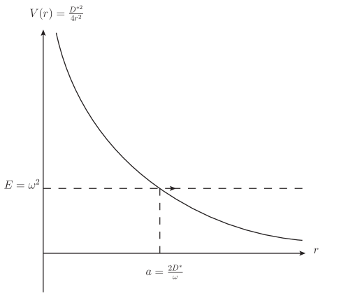
Figure 1: Potential for allowed and disallowed regions .

The most general WKB solution to this equation in the classically disallowed region is given by

$$\begin{split}\psi(\omega,r)=~{}&\frac{\sqrt{D^{*}}B}{\sqrt{2}\left(\frac{D^{*2}}{4r^{2}}-\omega^{2}\right)^{\frac{1}{4}}}\left(\frac{D^{*}}{2\omega r}-\sqrt{\frac{D^{*2}}{4\omega^{2}r^{2}}-1}\right)^{-\frac{D^{*}}{2}}\left(\frac{D^{*}}{\omega}\right)^{-\frac{D^{*}}{2}}e^{\frac{D^{*}}{2}-\sqrt{\frac{D^{*2}}{4}-\omega^{2}r^{2}}}\\ +&\frac{\sqrt{D^{*}}A}{\sqrt{2}\left(\frac{D^{*2}}{4r^{2}}-\omega^{2}\right)^{\frac{1}{4}}}\left(\frac{D^{*}}{2\omega r}-\sqrt{\frac{D^{*2}}{4\omega^{2}r^{2}}-1}\right)^{\frac{D^{*}}{2}}\left(\frac{D^{*}}{\omega}\right)^{-\frac{D^{*}}{2}}e^{\frac{D^{*}}{2}+\sqrt{\frac{D^{*2}}{4}-\omega^{2}r^{2}}}.\end{split}$$ (403)

In the limit $2r\omega\ll D^{*}$ this solution reduces to

$$\psi(\omega,r)=\frac{B}{r^{\frac{D-4}{2}}}+A\left(\frac{e\omega}{D}\right)^{D-3}r^{\frac{D-2}{2}},$$ (404)

in agreement with (30). In order to obtain (404) , we have used $D^{*}=\left(D-3\right)+{\cal O}(1/D)$ and have ignored this higher order correction. We have also used

$$\Omega_{n}=\frac{2\pi^{\frac{n+1}{2}}}{\Gamma(\frac{n+1}{2})}.$$ (405)

In the classically allowed region, on the other hand,

$$\psi(\omega,r)=\frac{Ee^{i{\frac{D^{*}\pi}{4}}}e^{-i\frac{D^{*}}{2}\sin^{-1}\left(\frac{D^{*}}{2\omega r}\right)}e^{-i\sqrt{\omega^{2}r^{2}-\frac{D^{*2}}{4}}}+Ce^{-i{\frac{D^{*}\pi}{4}}}e^{i\frac{D^{*}}{2}\sin^{-1}\left(\frac{D^{*}}{2\omega r}\right)}e^{i\sqrt{\omega^{2}r^{2}-\frac{D^{*2}}{4}}}}{\left(\omega^{2}-\frac{D^{*2}}{4r^{2}}\right)^{\frac{1}{4}}}.$$ (406)

In the limit $2\omega r\gg D^{*}$ (406) reduces to

$$\psi(\omega,r)=\frac{1}{\sqrt{\omega}}\left(Ee^{i{\frac{D^{*}\pi}{4}}}e^{-i\omega r}+Ce^{-i{\frac{D^{*}\pi}{4}}}e^{i\omega r}\right),$$ (407)

in agreement with (32).

The usual WKB crossing formulae relate the four constants $A$ $B$ $C$ $E$. Using Equation 7.35 of Merzbacher:1998rr we have

$$\begin{split}C&=e^{-\frac{i\pi}{4}}\left(A+\frac{iB}{2}\right)\sqrt{\frac{D^{*}}{2}}\left(\frac{D^{*}}{\omega}\right)^{-\frac{D^{*}}{2}}e^{\frac{D^{*}}{2}},\\ E&=e^{\frac{i\pi}{4}}\left(A-\frac{iB}{2}\right)\sqrt{\frac{D^{*}}{2}}\left(\frac{D^{*}}{\omega}\right)^{-\frac{D^{*}}{2}}e^{\frac{D^{*}}{2}}.\end{split}$$ (408)

As we have explained in the main text, the constant $B$ is universal and is given by $B=\frac{1}{(D-3)\Omega_{D-2}}$. If we now specialize to the case of the retarded Greens function we have $E=0$. From (408) it follows that

$$\begin{split}C&=\frac{(1+i)}{\sqrt{2}}B\sqrt{\frac{D^{*}}{2}}\left(\frac{D^{*}}{\omega}\right)^{-\frac{D^{*}}{2}}e^{\frac{D^{*}}{2}}=\frac{(1+i)}{\sqrt{2}}\left(2\right)^{-\frac{D}{2}}\frac{\omega^{\frac{D-3}{2}}}{\pi^{\frac{D-2}{2}}},\\ A&=\frac{iB}{2}=\frac{i}{2(D-3)\Omega_{D-2}}.\end{split}$$ (409)

It follows that in the classically allowed region

$$\psi(\omega,r)=-\left(2i\right)^{-\frac{D^{*}}{2}}\frac{\omega^{\frac{D-3}{2}}}{\pi^{\frac{D-2}{2}}}\frac{e^{i\left(\sqrt{\omega^{2}r^{2}-\frac{D^{*2}}{4}}+\frac{D^{*}}{2}\sin^{-1}\left(\frac{D^{*}}{2\omega r}\right)\right)}}{\left(\omega^{2}-\frac{D^{*2}}{4r^{2}}\right)^{\frac{1}{4}}}.$$ (410)

It is easily verified that (410) matches both the leading and first subleading terms in (22) when expanded at large $r$.

In the classically disallowed region , where $D^{*}>2{\omega}r$ we find the explicit formula

$$\begin{split}\psi(\omega,r)=&~{}\frac{1}{(D-3)\Omega_{D-2}}\bigg{(}\frac{e^{\frac{D^{*}}{2}-\sqrt{\frac{D^{*2}}{4}-\omega^{2}r^{2}}}}{\left(\frac{D^{*2}}{4r^{2}}-\omega^{2}\right)^{\frac{1}{4}}}\left(\frac{D^{*}}{\omega}\left(\frac{D^{*}}{2\omega r}-\sqrt{\frac{D^{*2}}{4\omega^{2}r^{2}}-1}\right)\right)^{-\frac{D^{*}}{2}}\\ &~{}~{}~{}~{}~{}~{}~{}~{}~{}~{}~{}~{}~{}~{}~{}~{}~{}~{}~{}~{}+\frac{i}{2}\frac{e^{\frac{D^{*}}{2}+\sqrt{\frac{D^{*2}}{4}-\omega^{2}r^{2}}}}{\left(\frac{D^{*2}}{4r^{2}}-\omega^{2}\right)^{\frac{1}{4}}}\left(\frac{1}{2r}-\sqrt{\frac{1}{4r^{2}}-\frac{\omega^{2}}{D^{*2}}}\right)^{\frac{D^{*}}{2}}\bigg{)}\\ =&\frac{1}{(D-3)\Omega_{D-2}}\left(\frac{1}{r^{\frac{D-4}{2}}}+\frac{i}{2}\left(\frac{e\omega}{D}\right)^{D-3}{r^{\frac{D-2}{2}}}\right),\end{split}$$ (411)

where the second expression applies at small $\omega r$. So the Greens Function can be written as

$$G(\omega,r)=\frac{1}{(D-3)\Omega_{D-2}r^{\frac{D-3}{2}}}\left(\frac{1}{r^{\frac{D-3}{2}}}+\frac{i}{2}\left(\frac{e\omega}{D}\right)^{D-3}{r^{\frac{D-3}{2}}}\right).$$ (412)

It may be verified that this result matches the small $r$ asymptotics of the exact formula (20) in the following sense. From (20) the exact Greens function is given by

$$G(\omega,r)=\frac{i}{4}\left(\frac{\omega}{2\pi r}\right)^{\frac{D-3}{2}}\left(J_{\frac{D-3}{2}}(\omega r)+iN_{\frac{D-3}{2}}(\omega r)\right),$$ (413)

where $N_{n}$ is the Neumann function. At small $\omega r$ we use the small $\omega r$ expansion of the Bessel and Neumann functions to obtain

$$\begin{split}G(\omega,r)&=\frac{i}{4}\frac{1}{(D-3)\Omega_{D-2}}\left(\frac{\omega}{2\pi r}\right)^{\frac{D-2}{2}}\left(-4i\left(\frac{2\pi}{\omega r}\right)^{\frac{D-3}{2}}+\frac{2}{e}\left(\frac{2\pi e\omega r}{D}\right)^{\frac{D-3}{2}}\right)\\ &=\frac{1}{(D-3)\Omega_{D-2}r^{\frac{D-3}{2}}}\left(\frac{1}{r^{\frac{D-3}{2}}}+\frac{i}{2e}\left(\frac{e\omega}{D}\right)^{D-3}{r^{\frac{D-3}{2}}}\right),\end{split}$$ (414)

in agreement with (411).

We will now explain in what sense the WKB approximation may be thought of as the first term in a systematic large $D$ approximation of the Greens function. The first correction to any WKB approximation is of order of the fractional change in the wavenumber over a distance scale of order one wavelength. In formulae, the first correction to this approximation is of order $\frac{1}{k(r)}\partial_{r}\ln k(r)$ where $k(r)$ is the local WKB wave number. In the classically allowed region $k(r)=\sqrt{\omega^{2}-\frac{D^{2}}{4r^{2}}}$. So the fractional correction, $E(r)$, to the WKB approximation can be estimated to be of order

$$E(r)=\frac{\frac{{D^{*}}^{2}}{r^{3}}}{\left(\sqrt{\omega^{2}-\frac{{D^{*}}^{2}}{4r^{2}}}\right)^{3}}.$$

Provided that $\sqrt{\omega^{2}-\frac{{D^{*}}^{2}}{4r^{2}}}$ is of order unity (i.e. provided we don’t get too near the turning point) it follows that $E(r)={\cal O}\left(1/D\right)$ (recall that $\omega r>D/2$). This conclusion works all the way down to $\omega r-\frac{D}{2}\sim\frac{1}{D^{\frac{2}{3}}}$. In a similar manner the fractional error to the WKB approximation in the classically disallowed region is once again estimated as

$$E(r)\sim\frac{1}{D\sqrt{1-\frac{4\omega^{2}r^{2}}{D^{2}}}},$$

and is once again of order $\frac{1}{D}$ provided we stay away from the turning point. In summary, the WKB approximation provides an excellent approximation to the Greens function at large $D$ except within a distance of order $\frac{1}{D^{\frac{2}{3}}}$ of the turning point.

We end this subsection with a qualitative description of the retarded Green’s function in the large $D$ limit. There are four qualitatively distinct regions in the Greens function. Deep into the classically allowed region, for $r\omega\gg D^{2}$, the Greens function is in the radiation zone. In this regime (22) applies, and the modulus of Greens function is proportional to $\frac{e^{i\omega r}}{r^{\frac{D-2}{2}}}$. It follows that the mod squared Greens function is proportional to the inverse volume of the $D-2$ sphere of radius $r$ in this region, and so represents radiation whose integrated flux is independent of $r$.

Moving further in we reach the intermediate radiation zone $\frac{D}{2}<\frac{\omega r}{2}\ll D^{2}$. In this region the Greens function represents an oscillating radiation field that has not propagated far enough to settle into its large $r$ asymptotic value.

Moving to smaller $r$ we pass the turning point of the potential and enter the classically forbidden region. In this intermediate static regime $\sqrt{D}\ll\frac{\omega r}{2}\ll\frac{D}{2}$, $\psi$ no longer oscillates as a function of $r$. Instead the Greens function turns into a sum of a term that grows as $r$ increases and another that decays as $r$ decreases. The decaying and growing pieces are comparable in magnitude near the turning point. However the decaying term grows towards small $r$ and quickly dominates.

Moving to still smaller $r$ we reach the static zone $\frac{\omega r}{2}\ll\sqrt{D}$. In this region the first of (22) applies, and $G(\omega,r)$ becomes independent of $\omega$ (justifying the name static zone). The decaying term in (411) is much larger than the growing term in this region; in particular the the ratio of the growing term to the decaying term of order $\frac{1}{D^{D}}$ when $\omega r$ is of order unity.

Appendix F Action of the Greens function on scalars, vectors and tensors in a spherical basis

F.0.1 Results for the off centred Green’s function

In our analysis of radiation we will will find it useful to have a generalization of the exact expression (20) to a Greens function whose source point is displaced away from the origin. In the next subsection we demonstrate that

$$G(\omega,|{\vec{r}}-{\vec{r}}^{\prime}|)=\frac{i\pi}{2}\sum_{l=0}^{\infty}\frac{1}{(r^{\prime}r)^{\frac{D-3}{2}}}H_{\frac{D-3+2l}{2}}^{(1)}(\omega r)J_{\frac{D-3+2l}{2}}(\omega r^{\prime}){\mathcal{P}}_{l}(\theta,\theta^{\prime}).$$ (415)

This result applies provided $|r|>|r^{\prime}|^{\prime}$, i.e. provided that the observation point is located further from the origin than the source point. The Hankel function $H^{(1)}(r)$ which appears in (238) is the unique solution to the Bessel function that is is purely outgoing at infinity. On the other hand the Bessel function $J(r^{\prime})$ that also appears in this expression is the unique solution to the Bessel equation that is regular at the origin. $\theta$ collectively denotes all the angles of the point ${\vec{r}}$ on $S^{D-2}$, $\theta^{\prime}$ similarly denotes all angles of the point ${\vec{r}^{\prime}}$ and $\mathcal{P}_{l}(\theta,\theta^{\prime})$ is the projector onto the angular dependence of the $l^{th}$ spherical harmonic defined in (349).

It is easily verified that (238) reduces to (20) in the limit $r^{\prime}\to 0$. As a consistency check on this formula we have explicitly verified that the expansion (238) is translationally invariant, i.e. that

$$(\partial_{{\vec{r}}}+\partial_{{\vec{r}}^{\prime}})G(\omega,|{\vec{r}}-{\vec{r}}^{\prime}|)=0.$$ (416)

Note also that in the limit $\omega\rightarrow 0$,

$$G(0,|\vec{r}-\vec{r}^{\prime}|)=\frac{1}{r^{D-3}}\sum_{l=0}^{\infty}\left(\frac{r^{\prime}}{r}\right)^{l}\frac{1}{2l+D-3}{\mathcal{P}}_{l}(\theta,\theta^{\prime}).$$ (417)

F.0.2 Derivation

The expression (238) may be derived as follows. Provided that ${\vec{r}}\neq{\vec{r}}^{\prime}$ (and so in particular when $|{\vec{r}}|>|{\vec{r}}^{\prime}|$ ) the Greens function is annihilated by the action of

$$\left(\omega^{2}+{\vec{\nabla}}^{2}\right),$$

separately on the variables ${\vec{r}}$ and ${\vec{r}}^{\prime}$. The most general solution of the equation

$$\left(\omega^{2}+{\vec{\nabla}}^{2}\right)\phi(\omega,\vec{r})=0,$$ (418)

is a linear superposition of modes of the form $\phi_{l}(\omega,r)Y_{lm}(\theta)$ , where $Y_{lm}$ represents an arbitrary scalar spherical harmonic in the representation $(l,0,0,\ldots,0)$ of $SO(D-1)$. Using the fact that

$$\nabla^{2}Y_{lm}=-l(l+D-3)Y_{lm},$$ (419)

where the Laplacian is taken on the unit sphere, see (348)) it follows from (418) that

$$\left(\omega^{2}+\frac{1}{r^{D-2}}\partial_{r}(r^{D-2}\partial_{r})-\frac{l(l+D-3)}{r^{2}}\right)\phi_{l}(\omega,r)=0.$$ (420)

Solving this equation we find that

$$\phi_{l}(\omega,r)=\frac{1}{r^{\frac{D-3}{2}}}\left(A_{l,\omega}H_{\frac{D-3+2l}{2}}^{(1)}(\omega r)+B_{l,\omega}J_{\frac{D-3+2l}{2}}(\omega r)\right).$$ (421)

The boundary conditions on our Greens function require it to be regular at every finite value of ${\vec{r}}^{\prime}$ other than ${\vec{r}}$; and requires the Greens function to be an outgoing function of ${\vec{r}}$; these considerations force us to use the Hankel function with argument $r$ and the Bessel function with argument $r^{\prime}$. The Greens function must also be rotationally invariant under simultaneous rotations of $\theta$ and $\theta^{\prime}$. As we have explained above, the unique rotationally invariant function of two angles constructed using functions only in in the $l^{th}$ spherical harmonic sector is the projector ${\cal P}_{l}$ defined in (349). It follows from all these considerations that the Greens function must be given by an expression of the form

$$G(\omega,|{\vec{r}}-{\vec{r}}^{\prime}|)=\sum_{l=0}^{\infty}\frac{a_{l}}{(r^{\prime}r)^{\frac{D-3}{2}}}H_{\frac{D-3+2l}{2}}^{(1)}(\omega r)J_{\frac{D-3+2l}{2}}(\omega r^{\prime}){\cal P}_{l}(\theta,\theta^{\prime}),$$ (422)

for some as yet unknown coefficients $a_{l}$. We will now demonstrate that

$$a_{l}=\frac{i\pi}{2};~{}~{}~{}{\rm for~{}all~{}}l$$ (423)

using which (238) follows.

In order to obtain (423) we use the large argument expansion of the Hankel function (21). (422) simplifies to

$$G(\omega,|{\vec{r}}-{\vec{r}}^{\prime}|)\approx i\sqrt{\frac{\pi}{2}}\left(\frac{-i\omega}{r}\right)^{\frac{D-2}{2}}e^{i\omega r}\sum_{l}J_{\frac{D-3+2l}{2}}(\omega r^{\prime})(\omega r^{\prime})^{-\frac{D-3}{2}}{\cal P}_{l}(\theta,\theta^{\prime})$$ (424)

We also specialize (422) to the case in which the source and observation points are at the same angle. In this special case the LHS of (238) is simply $G(\omega,(r-r^{\prime}))$ (see (20)) and (422) reduces to

$$G(\omega,(r-r^{\prime}))=\sum_{l=0}^{\infty}\frac{a_{l}{\mathcal{P}}_{l}(0)}{(r^{\prime}r)^{\frac{D-3}{2}}}H_{\frac{D-3+2l}{2}}^{(1)}(\omega r)J_{\frac{D-3+2l}{2}}(\omega r^{\prime})$$ (425)

(where $G(\omega,r)$ is defined in (20) and ${\mathcal{P}}_{l}(0)$ is presented in (354)). In order to determine the coefficients $a_{l}$ it is sufficient to further specialize (425) to large $r$ and retain only leading order terms on both sides in the $\frac{1}{r}$ expansion. (425) reduces to

$$\begin{split}&\frac{i}{4}\left(\frac{\omega}{2\pi r}\right)^{\frac{D-3}{2}}\left(i^{-\frac{D-2}{2}}\sqrt{\frac{2}{\pi\omega r}}e^{i\omega(r-r^{\prime})}\right)\\ &=i^{-\frac{D-2}{2}}\sqrt{\frac{2}{\pi\omega r}}\left(\frac{\omega}{r}\right)^{\frac{D-3}{2}}\frac{e^{i\omega r}}{\omega}\sum_{l}i^{-l}a_{l}{\mathcal{P}}_{l}(0)J_{\frac{D-3+2l}{2}}(\omega r^{\prime})(\omega r^{\prime})^{-\frac{D-3}{2}}\\ &{\rm i.e.}~{}~{}~{}e^{ix}=-4i(2\pi)^{\frac{D-3}{2}}\sum_{l}a_{l}{\mathcal{P}}_{l}(0)J_{\frac{D-3+2l}{2}}(x)(x)^{\frac{D-3}{2}}\\ \end{split}$$ (426)

(where we have used (22), and $x=\omega r^{\prime}$). Taylor expanding the LHS and RHS in $x$ about $x=0$ and using the well known series expansion for the Bessel function

$$J_{\frac{D-3+2l}{2}}(x)(x)^{\frac{D-3}{2}}=\sum_{m=0}^{\infty}\frac{(-1)^{m}}{m!\Gamma\left(l+m+\frac{D-1}{2}\right)}\frac{(x)^{l+2m}}{2^{l+2m+\frac{D-3}{2}}},$$ (427)

we find the following recursion relations

$$\tilde{a}_{n}=\Gamma\left(n+\frac{D-1}{2}\right)\left(\frac{2^{n}}{n!}-\sum_{m=1}^{\lfloor\frac{n}{2}\rfloor}\frac{\tilde{a}_{n-2m}}{m!~{}\Gamma\left(n-m+\frac{D-1}{2}\right)}\right),$$ (428)

where

$$\tilde{a}_{l}=-4i\pi^{\frac{D-3}{2}}{\cal P}_{l}(0)a_{l}.$$ (429)

Using the explicit value of ${\cal P}_{l}(0)$ listed in (354) it may be verified that

$$a_{l}=\frac{i\pi}{2},$$ (430)

solves the recursion relation (428), establishing (423).

F.1 Action of the retarded Greens function on the arbitrary spherically decomposed vector field

We will now use the results the previous subsections together with those of Appendix D to present the general solution to the equation

$$\left(-\nabla^{2}-\omega^{2}\right){\vec{E}}={\vec{J}}_{\rm eff},$$ (431)

where the field $J_{\rm eff}$ is a general vector field in $R^{D-1}$ that admits the expansion (370). We search for the unique solution to this problem subject to the restriction that it behaves as $e^{i\omega r}$ at infinity.

In Cartesian coordinates the solution to this problem is simply given by

$${\vec{E}}({\vec{r}})=\int dr^{\prime}G(\omega,|{\vec{r}}-{\vec{r}}^{\prime}|){\vec{J}}_{\rm eff}(r^{\prime}),$$ (432)

where the Green’s function $G(\omega,|{\vec{r}}-{\vec{r}}^{\prime}|)$ was defined in (238). Using (373) the solution (432) can be rewritten in terms of a spherical decomposition as

$${\vec{E}}(\omega,{\vec{r}})={\vec{\mathcal{A}}}^{-}[\xi_{\alpha}]+{\vec{\mathcal{A}}}^{+}[\xi_{\beta}]+\vec{\upsilon}_{\gamma},$$ (433)

where

$$\begin{split}\xi_{\alpha}(\omega,{\vec{r}})&=\sum_{l}\frac{i\pi}{2}\frac{H^{(1)}_{\frac{D-3+2(l-1)}{2}}(\omega r)}{r^{\frac{D-3}{2}}}\int dr^{\prime}J_{\frac{D-3+2(l-1)}{2}}(\omega r^{\prime})~{}r^{\prime\frac{D-1}{2}}\alpha_{l}(\omega,r^{\prime},\theta),\\ \xi_{\beta}(\omega,{\vec{r}})&=\sum_{l}\frac{i\pi}{2}\frac{H^{(1)}_{\frac{D-3+2(l+1)}{2}}(\omega r)}{r^{\frac{D-3}{2}}}\int dr^{\prime}J_{\frac{D-3+2(l+1)}{2}}(\omega r^{\prime})~{}r^{\prime\frac{D-1}{2}}\beta_{l}(\omega,r^{\prime},\theta),\\ {\vec{\upsilon}}_{\gamma}(\omega,{\vec{r}})&=\sum_{l}\frac{i\pi}{2}\frac{H^{(1)}_{\frac{D-3+2l}{2}}(\omega r)}{r^{\frac{D-3}{2}}}\int dr^{\prime}J_{\frac{D-3+2l}{2}}(\omega r^{\prime})~{}r^{\prime\frac{D-1}{2}}{\vec{\gamma}}_{l}(\omega,r^{\prime},\theta).\\ \end{split}$$ (434)

F.2 Action of the retarded Greens function on the arbitrary spherically decomposed tensor field

In this brief subsection we study the equation

$$\left(-\nabla^{2}-\omega^{2}\right){{\cal H}_{ij}}=T_{ij},$$ (435)

where $T_{ij}$ is a given symmetric tensor field. We will find the unique solution to (435) subject to the condition that ${\cal H}_{ij}$ is outgoing at infinity.

Let the source function $T_{ij}$ have the spherical decomposition listed in (379). Proceeding as in the previous subsection, it is easy to verify that the unique outgoing solution to (435) is given by

$${\cal H}_{ij}(\omega,{\vec{r}})={\mathcal{C}}_{ij}^{-}[\xi_{\alpha}]+{\mathcal{C}}_{ij}^{+}[\xi_{\beta}]+{\mathcal{C}}_{ij}^{0}[\xi_{\gamma}]+\delta_{ij}\xi_{\kappa}+{\mathcal{B}}_{ij}^{-}[\vec{\upsilon}_{\phi}]+{\mathcal{B}}_{ij}^{+}[\vec{\upsilon}_{\psi}]+\tau^{\chi}_{ij},$$ (436)

where

$$\begin{split}\xi_{\alpha}(\omega,{\vec{r}})&=\sum_{l}\frac{i\pi}{2}\frac{H^{(1)}_{\frac{D-3+2(l-2)}{2}}(\omega r)}{r^{\frac{D-3}{2}}}\int dr^{\prime}J_{\frac{D-3+2(l-2)}{2}}(\omega r^{\prime})~{}r^{\prime\frac{D-1}{2}}\alpha_{l}(\omega,r^{\prime},\theta),\\ \xi_{\beta}(\omega,{\vec{r}})&=\sum_{l}\frac{i\pi}{2}\frac{H^{(1)}_{\frac{D-3+2(l+2)}{2}}(\omega r)}{r^{\frac{D-3}{2}}}\int dr^{\prime}J_{\frac{D-3+2(l+2)}{2}}(\omega r^{\prime})~{}r^{\prime\frac{D-1}{2}}\beta_{l}(\omega,r^{\prime},\theta),\\ \xi_{\gamma}(\omega,{\vec{r}})&=\sum_{l}\frac{i\pi}{2}\frac{H^{(1)}_{\frac{D-3+2l}{2}}(\omega r)}{r^{\frac{D-3}{2}}}\int dr^{\prime}J_{\frac{D-3+2l}{2}}(\omega r^{\prime})~{}r^{\prime\frac{D-1}{2}}\gamma_{l}(\omega,r^{\prime},\theta),\\ \xi_{\kappa}(\omega,{\vec{r}})&=\sum_{l}\frac{i\pi}{2}\frac{H^{(1)}_{\frac{D-3+2l}{2}}(\omega r)}{r^{\frac{D-3}{2}}}\int dr^{\prime}J_{\frac{D-3+2l}{2}}(\omega r^{\prime})~{}r^{\prime\frac{D-1}{2}}\kappa_{l}(\omega,r^{\prime},\theta),\\ \vec{\upsilon}_{\phi}(\omega,{\vec{r}})&=\sum_{l}\frac{i\pi}{2}\frac{H^{(1)}_{\frac{D-3+2(l-1)}{2}}(\omega r)}{r^{\frac{D-3}{2}}}\int dr^{\prime}J_{\frac{D-3+2(l-1)}{2}}(\omega r^{\prime})~{}r^{\prime\frac{D-1}{2}}\vec{\phi}_{l}(\omega,r^{\prime},\theta),\\ \vec{\upsilon}_{\psi}(\omega,{\vec{r}})&=\sum_{l}\frac{i\pi}{2}\frac{H^{(1)}_{\frac{D-3+2(l+1)}{2}}(\omega r)}{r^{\frac{D-3}{2}}}\int dr^{\prime}J_{\frac{D-3+2(l+1)}{2}}(\omega r^{\prime})~{}r^{\prime\frac{D-1}{2}}\vec{\chi}_{l}(\omega,r^{\prime},\theta),\\ \tau^{\chi}_{ij}(\omega,{\vec{r}})&=\sum_{l}\frac{i\pi}{2}\frac{H^{(1)}_{\frac{D-3+2l}{2}}(\omega r)}{r^{\frac{D-3}{2}}}\int dr^{\prime}J_{\frac{D-3+2l}{2}}(\omega r^{\prime})~{}r^{\prime\frac{D-1}{2}}(\chi_{l})_{ij}(\omega,r^{\prime},\theta).\end{split}$$ (437)

Appendix G Details relating to the general theory of radiation

G.1 Static Limit of Electromagnetic Radiation

It is useful to separately consider the scalar part of the electric field (first line of (259)) and the vector part (second line of (259)). Let us first focus on the scalar part of this field. Using (261) and the fact that $H_{n}(x)\sim x^{-n}$ , we see that the first term in the first line of (259) is negligible compared to the second term in the same line and at small $\omega$ and we find

$$\begin{split}{\vec{E}}(\omega,\vec{x})&=\sum_{l=0}^{\infty}\left(\frac{H_{\frac{D+2l-1}{2}}(\omega r)}{r^{\frac{D-3}{2}}}{\vec{\cal A}}^{+}[S^{+}_{l}(\omega,\theta)]\right)\\ &=\frac{-i}{\pi}\sum_{l=0}^{\infty}\left(2^{\frac{2l+D-1}{2}}\frac{\Gamma\left(\frac{2l+D-1}{2}\right)\left((l+D-3)\hat{r}S^{+}_{l}-r\vec{\tilde{\nabla}}S^{+}_{l}\right)}{\omega^{\frac{2l+D-1}{2}}r^{l+D-2}}\right)\\ &=-\vec{\nabla}\Phi^{E},\end{split}$$ (438)

where

$$\Phi^{E}=\frac{-i}{\pi}\sum_{l=0}^{\infty}\left(2^{\frac{2l+D-1}{2}}\frac{\Gamma\left(\frac{2l+D-1}{2}\right)}{\omega^{\frac{2l+D-1}{2}}}\frac{S^{+}_{l}}{r^{l+D-3}}\right),$$ (439)

$$\begin{split}S^{+}_{l}&=\frac{i\pi}{2}\int dr^{\prime}(r^{\prime})^{\frac{D-1}{2}}J_{\frac{2l+D-1}{2}}(\omega r^{\prime})\mathfrak{b}_{l}(\omega,r^{\prime},\theta)\\ &=\frac{i\pi}{2}\frac{\omega^{\frac{2l+D-1}{2}}}{2^{\frac{2l+D-1}{2}}\Gamma\left(\frac{2l+D+1}{2}\right)}\int dr^{\prime}(r^{\prime})^{l+D-1}\mathfrak{b}_{l}(\omega,r^{\prime},\theta).\end{split}$$ (440)

(438) is simply the statement that the electric field in the stationary limit is the gradient of a scalar potential. There is, of course, a simple explanation and interpretation of this fact. Recall that t he effective source ${\vec{\mathcal{J}}}_{eff}$ - from which $\mathfrak{b}$ is built - is a linear combination of two terms. One of the two terms is the time derivative of the spatial current, and is subleading compared to the other term (the spatial derivative of the charge current) in the small $\omega$ limit. In this limit, consequently, the formula for the electric field reduces to

$$\begin{split}{\vec{E}}&=\int G(\omega\to 0,|{\vec{r}}-{\vec{r}}^{\prime}|\nabla^{\prime}{\mathcal{J}}_{0}(r^{\prime})\\ &=\nabla\left(\int G(\omega\to 0,|{\vec{r}}-{\vec{r}}^{\prime}|{\mathcal{J}}_{0}(r^{\prime})\right)\\ &=-\nabla\Phi_{E},\\ &\Phi_{E}=-\int G(\omega\to 0,|{\vec{r}}-{\vec{r}}^{\prime}|{\mathcal{J}}_{0}(r^{\prime}).\end{split}$$ (441)

This is simply Coulomb’s law. Indeed it may directly be verified that $\Phi_{E}$ defined in (439) and (441) agree with each other. .

In the static limit magnetic field can be written using the Bianchi identity as:

$$F_{ij}(0,r,\theta)=\lim_{\omega\to 0}\frac{i(\nabla_{i}{\vec{E}}_{j}(\omega,r,\theta)-\nabla_{j}{\vec{E}}_{i}(\omega,r,\theta))}{\omega}.$$ (443)

The only term in (263) that contributes to the RHS of (443) is the pure vector piece $\mathfrak{c}$, which only receives contributions from the the term in ${\vec{\mathcal{J}}}_{eff}$ equal to $\partial_{0}{\vec{\mathcal{J}}}$.

In the limit of small $\omega$ ${\tilde{\vec{\mathfrak{c}}}}$ and ${\vec{\mathfrak{c}}}$ differ only by a factor of $\omega$ at it is easily verified that

$$\begin{split}F_{ij}(\omega,r,\theta)&=(\nabla_{i}{\vec{A}}_{j}(\omega,r,\theta)-\nabla_{j}{\vec{A}}_{i}(\omega,r,\theta)),\\ &{\vec{A}}=\lim_{\omega\to 0}\frac{i\vec{E}}{\omega}\\ \therefore&{\vec{A}}=\sum_{l}\frac{i}{(2l+D-3)r^{D-3}}\int dr^{\prime}(r^{\prime})^{D-2}\left(\frac{r^{\prime}}{r}\right)^{l}({\tilde{\vec{\mathfrak{c}}}}_{l}(0,r^{\prime},\theta)).\end{split}$$ (444)

In other words the magnetic field is given by $dA$ where $\nabla^{2}{\vec{A}}={\vec{\mathcal{J}}}$, and we recover the usual formulae of magnetostatics.

G.2 Constraints from current conservation and $\nabla\cdot E=0$

As we have explained in the main text the fact that $\nabla.{\vec{E}}$ vanishes in vacuum implies that the scalar functions ${\mathcal{S}}^{\pm}$ that characterize a general radiation field (see (259)) are not independent but are related by (261). In (264), however, we have presented separate formulae for ${\mathcal{S}}^{\pm}$ in terms of integrals over scalar components of charge currents. The consistency of (264) requires that these results for ${\mathcal{S}}^{\pm}$ automatically obey (261). We will now demonstrate that this is indeed the case.

At the structural level the way this works is very simple. If we take the divergence of (256) and use (265) we obtain (266), which guarantees that $\nabla.E$ vanishes in vacuum. In this section we will rerun this structural argument on the explicit formulae (264). The fact that we land on our feet serves as a consistency check of the algebra that led to (264) and (261).

In the rest of this subsection we proceed to algebraically demonstrate that

• The equation $\nabla\cdot E=0$ implies that the coefficient functions in (259) obey (261)

• That the relations (264) automatically obey (261) once we account for the fact that the current is conserved.

Demonstration that $\nabla\cdot E=0$ implies (261)

According to (259) the vacuum electromagnetic solution is given by

$$\vec{E}=\sum_{l}\left(\frac{H^{(1)}_{l+\frac{D-5}{2}}(\omega r)}{r^{\frac{D-3}{2}}}\vec{\mathcal{A}^{-}}[S^{-}_{l}(\omega,\theta)]+\frac{H^{(1)}_{l+\frac{D-1}{2}}(\omega r)}{r^{\frac{D-3}{2}}}\vec{\mathcal{A}^{+}}[S^{+}_{l}(\omega,\theta)]+\frac{H^{(1)}_{l+\frac{D-3}{2}}(\omega r)}{r^{\frac{D-3}{2}}}\vec{V}_{l}(\omega,\theta)\right).$$ (445)

Using

$$\begin{split}\nabla\cdot\vec{\mathcal{A}}^{-}[S^{-}_{l}(\omega,\theta)]&=lr^{l-1}\partial_{r}\left(\frac{H^{(1)}_{l+\frac{D-5}{2}}(\omega r)}{r^{l+\frac{D-5}{2}}}\right)S^{-}_{l}(\omega,\theta)\\ &=-lS^{-}_{l}(\omega,\theta)\frac{H^{(1)}_{l+\frac{D-3}{2}}(\omega r)}{r^{\frac{D-3}{2}}}\\ \nabla\cdot\vec{\mathcal{A}}^{+}[S^{+}_{l}(\omega,\theta)]&=\frac{l+D-3}{r^{l+D-2}}\partial_{r}\left(H^{(1)}_{l+\frac{D-1}{2}}(\omega r)r^{l+\frac{D-1}{2}}\right)S^{+}_{l}(\omega,\theta)\\ &=+(l+D-3)S^{+}_{l}(\omega,\theta)\frac{H^{(1)}_{l+\frac{D-3}{2}}(\omega r)}{r^{\frac{D-3}{2}}}\\ \nabla\cdot\vec{V}_{l}(\omega,\theta)&=0,\end{split}$$ (446)

it follows that $\nabla\cdot E=0$ provided

$$-lS^{-}_{l}(\omega,\theta)+(l+D-3)S^{+}_{l}(\omega,\theta)=0.$$ (447)

Proof that current conservation satisfies this requirement

Recall that according to (263) the effective current admits the following decomposition

$$\vec{\mathcal{J}}_{eff}=\sum_{l}\left(\mathcal{A}^{-}[\mathfrak{a}_{l}(\omega,r^{\prime},\theta^{\prime})]+\mathcal{A}^{+}[\mathfrak{b}_{l}(\omega,r^{\prime},\theta^{\prime})]+\vec{\mathfrak{c}}_{l}(\omega,r^{\prime},\theta^{\prime})\right).$$ (448)

Using (378) yields

$$\nabla^{\prime}\cdot\vec{\mathcal{J}}_{eff}=\sum_{l}\left(l{r^{\prime}}^{l-1}\partial_{r^{\prime}}\left(\frac{\mathfrak{a}_{l}(\omega,r^{\prime},\theta^{\prime})}{{r^{\prime}}^{l-1}}\right)+\frac{l+D-3}{{r^{\prime}}^{l+D-2}}\partial_{r^{\prime}}\left(\mathfrak{b}_{l}(\omega,r^{\prime},\theta^{\prime}){r^{\prime}}^{l+D-2}\right)\right).$$ (449)

From (265) we conclude that

$$l{r^{\prime}}^{l-1}\partial_{r^{\prime}}\left(\frac{\mathfrak{a}_{l}(\omega,r^{\prime},\theta^{\prime})}{{r^{\prime}}^{l-1}}\right)+\frac{l+D-3}{{r^{\prime}}^{l+D-2}}\partial_{r^{\prime}}\left(\mathfrak{b}_{l}(\omega,r^{\prime},\theta^{\prime}){r^{\prime}}^{l+D-2}\right)-\Box^{\prime}(J_{0})_{l}=0.$$ (450)

Multiplying by $\frac{i\pi}{2}J_{l+\frac{D-3}{2}}(\omega r^{\prime}){r^{\prime}}^{\frac{D-1}{2}}$ integrating by parts w.r.t. $r^{\prime}$ and noting also that $\int dr^{\prime}\Box^{\prime}\left(J_{l+\frac{D-3}{2}}(\omega r^{\prime}){r^{\prime}}^{\frac{D-1}{2}}\right)=0$ we get ,

$$\frac{i\pi l}{2}\int dr^{\prime}J_{l+\frac{D-5}{2}}(\omega r^{\prime}){r^{\prime}}^{\frac{D-1}{2}}\mathfrak{a}_{l}(\omega,r^{\prime},\theta^{\prime})-\frac{i\pi(l+D-3)}{2}\int dr^{\prime}J_{l+\frac{D-1}{2}}(\omega r^{\prime}){r^{\prime}}^{\frac{D-1}{2}}\mathfrak{b}_{l}(\omega,r^{\prime},\theta^{\prime})=0$$ (451)

Which from (264) translates to

$$lS^{-}_{l}(\omega,\theta)-(l+D-3)S^{+}_{l}(\omega,\theta)=0.$$ (452)

G.3 Static Limit of Gravitational Radiation

It is useful to separately consider the scalar vector and tensor parts of the curvature given in (277).

Focusing first on the scalar part we see from (277), (281) and the fact that $h_{n}(x)\sim x^{-n}$ , that in the limit $\omega\to 0$ the scalar part of (277) reduces to

$$\begin{split}R_{0i0j}(\omega,\vec{x})&=\lim_{\omega\to 0}\sum_{l=0}^{\infty}\left(\frac{H_{\frac{D+2l+1}{2}}(\omega r)}{r^{\frac{D-3}{2}}}\mathcal{C}^{+}_{ij}[S^{+}_{l}(\omega,\theta)]\right)\\ &=\frac{-i}{\pi}\lim_{\omega\to 0}\sum_{l=0}^{\infty}\left(2^{\frac{2l+D+1}{2}}\frac{\Gamma\left(\frac{2l+D+1}{2}\right)\left((l+D-2)\hat{r}-r\vec{\tilde{\nabla}}\right)\left((l+D-3)\hat{r}S^{+}_{l}-r\vec{\tilde{\nabla}}S^{+}_{l}\right)}{\omega^{\frac{2l+D+1}{2}}r^{l+D-1}}\right)\\ &=\nabla_{i}\nabla_{j}\Phi^{G},\end{split}$$ (453)

where

$$\begin{split}\Phi^{G}&=\frac{-i}{\pi}\sum_{l=0}^{\infty}\left(2^{\frac{2l+D+1}{2}}\frac{\Gamma\left(\frac{2l+D+1}{2}\right)}{r^{l+D-3}}\right)\lim_{\omega\to 0}\frac{S^{+}_{l}}{\omega^{\frac{2l+D+1}{2}}}\\ &=\sum_{l=0}^{\infty}\frac{1}{(2l+D+1)r^{l+D-3}}\int dr^{\prime}(r^{\prime})^{l+D}\mathfrak{b}_{l}(0,r^{\prime},\theta),\end{split}$$ (454)

where we have used

$$\lim_{\omega\to 0}\frac{S^{+}_{l}}{\omega^{\frac{2l+D+1}{2}}}=\frac{i\pi}{2}\frac{1}{2^{\frac{2l+D+1}{2}}\Gamma\left(\frac{2l+D+3}{2}\right)}\int dr^{\prime}(r^{\prime})^{l+D}\mathfrak{b}_{l}(0,r^{\prime},\theta).$$ (455)

(454) is simply the statement that $R_{0i0j}$ in the stationary limit is the double gradient of a suitably scaled version of the Newtonian potential $\phi^{G}$. Indeed it is easily verified that $\phi^{G}$ is given by

$$\nabla^{2}\phi^{G}=-8\pi\left(\mathcal{T}_{00}+\frac{\mathcal{T}}{D-2}\right)$$ (456)

Let us now turn to the vector part of $R_{0i0j}$. Once again using (277), (281) and the small argument expansion of the Hankel function we see that the vector part of $R_{0i0j}$ simplifies to

$$\begin{split}R_{0i0j}(\omega,\vec{x})&=\sum_{l=0}^{\infty}\left(\frac{H_{\frac{D+2l-1}{2}}(\omega r)}{r^{\frac{D-3}{2}}}\mathcal{B}^{+}_{ij}[V^{+}_{l}(\omega,\theta)]\right)\\ &=\frac{-i}{\pi}\sum_{l=0}^{\infty}\left(2^{\frac{2l+D-1}{2}}\frac{\Gamma\left(\frac{2l+D-1}{2}\right)\left((l+D-3)\hat{r}_{i}(V^{+}_{l})_{j}-r\tilde{\nabla}_{i}(V^{+}_{l})_{j}\right)}{\omega^{\frac{2l+D-1}{2}}r^{l+D-2}}\right)+\{i\leftrightarrow j\}\\ &=-i\omega\left(\nabla_{i}A^{G}_{j}+\nabla_{j}A^{G}_{i}\right),\end{split}$$ (458)

so that (using the Bianchi identity)

$$\begin{split}R_{0ijk}&=\frac{i}{\omega}\left(\nabla_{j}R_{0i0k}-\nabla_{k}R_{0i0j}\right)\\ &=-\nabla_{i}\left(\nabla_{j}A^{G}_{k}-\nabla_{k}A^{G}_{j}\right),\end{split}$$ (459)

where

$$A^{G}_{i}=\frac{1}{2\pi}\left(\frac{2}{\omega}\right)^{\frac{2l+D+1}{2}}\Gamma\left(\frac{2l+D-1}{2}\right)\frac{(V^{+}_{l})_{i}}{r^{l+D-3}}.$$ (460)

It is easily verified that

$$\nabla^{2}A^{G}_{i}=-8\pi T_{0i}.$$

Note that ${\vec{A}}^{G}$ obeys the same equation obeyed by the ‘vector potential’ magnetostatics with the role of the current being played by $T_{0i}$. Indeed (459) asserts that $R_{0ijk}$ is proportional to $\nabla_{i}F^{G}_{jk}$ where $F^{G}_{jk}$ is the magnetic field constructed from the effective vector potential $A^{G}_{i}$.

Finally we turn to the tensor part of $R_{0i0j}$. It follows immediately from

$$\nabla^{2}R_{0i0j}=8\pi\omega^{2}T_{ij}$$

In the small $\omega$ limit the contribution of tensor sources to to $R_{ijkm}$ takes the form

$$\begin{split}R_{0ijk}&=\frac{i}{\omega}\left(\nabla_{j}R_{0i0k}-\nabla_{k}R_{0i0j}\right),\\ R_{ijkm}&=\frac{i}{\omega}\left(\nabla_{i}R_{0jkm}-\nabla_{j}R_{0ikm}\right)\\ &=\nabla_{i}\nabla_{k}\mathfrak{T}_{jm}+\nabla_{j}\nabla_{m}\mathfrak{T}_{ik}-\nabla_{j}\nabla_{k}\mathfrak{T}_{im}-\nabla_{i}\nabla_{m}\mathfrak{T}_{jk},\\ \mathfrak{T}_{ij}&=\frac{-R_{0i0j}}{\omega^{2}}.\end{split}$$ (461)

The tensor contribution from the source is

$$\mathfrak{z}_{ij}=-8\pi\omega^{2}\left(\mathcal{T}_{ij}-\delta_{ij}\frac{\mathcal{T}^{k}_{k}}{D-2}\right).$$ (462)

The scalar sector also contributes to $R_{ijkm}$, but its closed form is a bit ugly unlike the other beautiful results in this section, and that can be obtained from the scalar contribution to $R_{0i0j}$. We don’t present it here.

G.4 Tracelessness and divergenceless of gravitational radiation

In this subsection we rerun some of the discussion of section G.2 but this time in the context of gravitational radiation. In particular we will explain how the explicit gravitational radiation formulae ensure that gravitational radiation is traceless and divergence free. At the formal level these results follow immediately once we use that fact that when a box of something (e.g. $\Box\zeta$) is convoluted with Green’s function, the resulting integral vanishes. We will now use this fact to demonstrate

Result 1: Gravitational Radiation is traceless.

$$h_{ij}(\omega,\vec{x})=-\frac{2}{\omega^{2}}\int G(\omega,|\vec{x}-\vec{x}^{\prime}|)\hat{\mathcal{T}}_{ij}(\omega,\vec{x^{\prime}})d^{D-1}x^{\prime}.$$ (463)

Hence

$$h_{ij}\eta^{ij}(\omega,\vec{x})=-\frac{2}{\omega^{2}}\int G(\omega,|\vec{x}-\vec{x}^{\prime}|)(\eta^{ij}\hat{\mathcal{T}}_{ij}(\omega,\vec{x^{\prime}}))d^{D-1}x^{\prime}.$$ (464)

Using Conservation of stress tensor, we have

$$\eta^{ij}\hat{\mathcal{T}}_{ij}=-\Box^{\prime}\left(\mathcal{T}_{00}+\frac{\mathcal{T}}{D-2}\right),$$ (465)

hence the integration vanishes, i.e. $h_{ij}\eta^{ij}=0$

Result 2: Gravitational Radiation is divergenceless.
Taking spatial divergence of (463),

$$\begin{split}\partial_{i}h_{ij}(\omega,\vec{x})&=-\frac{2}{\omega^{2}}\partial_{i}\int G(\omega,|\vec{x}-\vec{x}^{\prime}|)\hat{\mathcal{T}}_{ij}(\omega,\vec{x^{\prime}})d^{D-1}x^{\prime}\\ &=-\frac{2}{\omega^{2}}\int G(\omega,|\vec{x}-\vec{x}^{\prime}|)\left(\partial_{i}\hat{\mathcal{T}}_{ij}(\omega,\vec{x^{\prime}})\right)d^{D-1}x^{\prime}.\end{split}$$ (466)

Using Conservation of stress tensor, we have

$$\partial_{i}^{\prime}\hat{\mathcal{T}}_{ij}=-\Box^{\prime}\left(i\omega\mathcal{T}_{0j}+\mathcal{T}_{00}+\frac{\mathcal{T}}{D-2}\right),$$ (467)

hence the integration vanishes, i.e. $\partial_{i}h_{ij}=0.$

Appendix H Variation of the first order gravitational counterterm action

In this brief Appendix we demonstrate that the variation of (97) yields the stress tensor (98).

Varying the first term inside the bracket in (97) we find

$$\begin{split}\int\delta\sqrt{{\cal R}}=&~{}\int\frac{\delta{\cal R}}{2\sqrt{{\cal R}}}\\ =&~{}\int\frac{1}{2\sqrt{{\cal R}}}\left[-{\cal R}_{\mu\nu}{\delta g}^{\mu\nu}+\hat{\nabla}_{\mu}\hat{\nabla}_{\nu}{\delta g}^{\mu\nu}-\hat{\nabla}^{2}{\delta g}\right]\\ =&~{}\int\frac{1}{2}\left[-\left(\frac{{\cal R}_{\mu\nu}}{\sqrt{{\cal R}}}\right)+\left(\hat{\nabla}_{\mu}\hat{\nabla}_{\nu}-g^{(in)}_{AB}\hat{\nabla}^{2}\right)\left(\frac{1}{\sqrt{{\cal R}}}\right)\right]{\delta g}^{\mu\nu}\\ =&~{}\int\frac{1}{2}\left[-\left(\frac{{\cal R}_{\mu\nu}}{\sqrt{{\cal R}}}\right)-g^{(in)}_{\mu\nu}\hat{\nabla}^{2}\left(\frac{1}{\sqrt{{\cal R}}}\right)+{\cal O}\left(\frac{1}{D}\right)\right]{\delta g}^{\mu\nu}\\ =&~{}\int\frac{1}{2}\left[-\left(\frac{{\cal R}_{\mu\nu}}{\sqrt{{\cal R}}}\right)+g^{(in)}_{\mu\nu}\left(\frac{\hat{\nabla}^{2}{\cal R}}{2{\cal R}^{\frac{3}{2}}}\right)+{\cal O}\left(\frac{1}{D}\right)\right]{\delta g}^{\mu\nu},\end{split}$$ (468)

where for convenience, we have used the notation $\delta g^{(ind)}_{\mu\nu}=\delta g_{\mu\nu}$ and we have used the formula

$$\begin{split}&\delta{\cal R}_{\mu\nu}=\frac{1}{2}\left[\hat{\nabla}_{\alpha}\hat{\nabla}_{\mu}{\delta g}^{\alpha}_{\nu}+\hat{\nabla}_{\alpha}\hat{\nabla}_{\nu}{\delta g}^{\alpha}_{\mu}-\hat{\nabla}_{\mu}\hat{\nabla}_{\nu}{\delta g}-\hat{\nabla}^{2}{\delta g}_{\mu\nu}\right]\\ \Rightarrow~{}&\delta{\cal R}=-{\delta g}^{\mu\nu}{\cal R}_{\mu\nu}+\left(\hat{\nabla}_{\mu}\hat{\nabla}_{\nu}-g^{(ind)}_{\mu\nu}\hat{\nabla}^{2}\right)h^{AB},\\ \text{where}~{}~{}&{\delta g}=g_{(ind)}^{\mu\nu}{\delta g}_{\mu\nu},~{}~{}\delta g^{\mu\nu}=g_{(ind)}^{\mu\alpha}~{}\delta g_{\alpha\beta}~{}g_{(ind)}^{\alpha\nu}.\end{split}$$ (469)

Varying the second term inside the bracket in (97) we find

$$\begin{split}&\frac{1}{2}~{}~{}\delta\left(\frac{{\cal R}_{\mu\nu}{\cal R}^{\mu\nu}}{{\cal R}^{\frac{3}{2}}}\right)\\ =&~{}-\frac{3}{4}{\cal R}^{-\frac{5}{2}}~{}{\cal R}_{\mu\nu}{\cal R}^{\mu\nu}~{}\delta{\cal R}-\frac{{\cal R}_{\mu\alpha}{\cal R}^{\alpha}_{\nu}~{}{\delta g}^{\mu\nu}}{{\cal R}^{\frac{3}{2}}}+\frac{{\cal R}^{\mu\nu}~{}\delta{\cal R}_{\mu\nu}}{{\cal R}^{\frac{3}{2}}}.\end{split}$$ (470)

Now from equation (469) it follows that

$$\begin{split}&\int{\cal R}^{-\frac{5}{2}}~{}{\cal R}_{\mu\nu}{\cal R}^{\mu\nu}~{}\delta R\\ =~{}&\int{\cal R}^{-\frac{5}{2}}~{}{\cal R}_{\alpha\beta}{\cal R}^{\alpha\beta}\left[-{\delta g}^{\mu\nu}{\cal R}_{\mu\nu}+\left(\hat{\nabla}_{\mu}\hat{\nabla}_{\nu}-g^{(ind)}_{\mu\nu}\hat{\nabla}^{2}\right){\delta g}^{\mu\nu}\right]\\ =~{}&\int{\delta g}^{\mu\nu}\left[-{\cal R}^{-\frac{5}{2}}~{}{\cal R}_{\alpha\beta}{\cal R}^{\alpha\beta}{\cal R}_{\mu\nu}+\left(\hat{\nabla}_{\mu}\hat{\nabla}_{\nu}-g_{\mu\nu}\hat{\nabla}^{2}\right)\left({\cal R}^{-\frac{5}{2}}~{}{\cal R}_{\alpha\beta}{\cal R}^{\alpha\beta}\right)\right]\\ =~{}&\int{\delta g}^{\mu\nu}\left[{\cal O}\left(\frac{1}{D}\right)\right]\end{split}.$$ (471)

Similarly the second term in equation (470) is also of order ${\cal O}\left(\frac{1}{D}\right)$. In the third term of equation (470) if we substitute the formula equation (469) we get one term which is of order ${\cal O}(1)$.

$$\begin{split}&\int\frac{{\cal R}^{\mu\nu}~{}\delta{\cal R}_{\mu\nu}}{{\cal R}^{\frac{3}{2}}}\\ =~{}&\int\left[-g^{(ind)}_{\mu\nu}\left(\frac{\hat{\nabla}_{\alpha}\hat{\nabla}_{\beta}{\cal R}^{\alpha\beta}}{R_{(in)}^{\frac{3}{2}}}\right)+{\cal O}\left(\frac{1}{D}\right)\right]\delta g^{\mu\nu}\\ =~{}&\int\left[-g^{(ind)}_{\mu\nu}\left(\frac{\hat{\hat{\nabla}}^{2}{\cal R}}{2{\cal R}^{\frac{3}{2}}}\right)+{\cal O}\left(\frac{1}{D}\right)\right]\delta g^{\mu\nu}.\end{split}$$ (472)

Using equation (468), (470), (471) and (472) we find the equation (98)

Appendix I Perturbative solution for $\rho$

In this section we find the solution of (100). In order to do this we find it convenient to use the following coordinate system. Choose any point on the membrane. We treat this point as the origin of our coordinate system. We now erect a Cartesian coordinate system about this point, making sure to orient a special coordinate, $z$, so that the normal to the membrane at that point is $dz$. Let the remaining Cartesian coordinates (which are all orthogonal to each other and to $z$ but are otherwise arbitrary) be denoted by $x^{\mu}$). It follows that, in this coordinate system, the equation of the membrane takes the following form

$$z(y_{\mu})=-\frac{K_{\mu\nu}}{2}y_{\mu}y_{\nu}-\frac{C_{\mu\nu\sigma}}{3}y_{\mu}y_{\nu}y_{\sigma}-\frac{D_{\mu\nu\sigma\rho}}{4}y_{\mu}y_{\nu}y_{\sigma}y_{\rho}+\cdots$$ (473)

Now consider a point outside the membrane whose coordinates are $(z,x_{\mu})$. At least in a neighbourhood of the membrane any such point may uniquely be associated with a point $(z(y_{\mu}),y_{\mu})$ on the membrane by the requirement that a straight line drawn normal through this membrane point passes through $(z,x_{\mu})$.

Let $y_{\mu}(z,x_{\mu})$ denote the coordinates of the membrane point associated with an arbitrary bulk point in this manner, and let $s(z,x_{\mu})$ denote the distance along this line from the given bulk point to the membrane. We will now determine $y_{\mu}(z,x_{\mu})$ and $s(z,x_{\mu})$ in a Taylor series expansion in $x_{\mu}$.

Working in a Taylor expansion in $y_{\mu}$, the normal at any point on the membrane is given by

$$n=\frac{dz+\left({K_{\mu\nu}}y_{\nu}+{C_{\mu\nu\sigma}}y_{\nu}y_{\sigma}+{D_{\mu\nu\sigma\rho}}y_{\nu}y_{\sigma}y_{\rho}\right)dy_{\mu}}{\mathcal{N}},$$ (474)

where the normalization $\mathcal{N}$ is chosen to ensure that $n.n=1$. To solve for $y_{\mu}$ in terms of the $x_{\mu}$ and $z$ we note that, by definition

$$\begin{split}\frac{x_{\mu}-y_{\mu}}{z-z_{0}}&=\frac{n_{\mu}}{n_{z}},\\ \frac{x_{\mu}-y_{\mu}}{z-z_{0}}&=\left(K_{\mu\nu}y_{\nu}+{C_{\mu\nu\sigma}}y_{\nu}y_{\sigma}+{D_{\mu\nu\sigma\rho}}y_{\nu}y_{\sigma}y_{\rho}\right).\end{split}$$ (475)

These equations are easily solved in a Taylor series expansion in $x_{\mu}$ (but to all orders in $z$). To the cubic order in $x_{\mu}$ we have

$$\begin{split}y_{\mu}&=(Px)_{\mu}-z(P\cdot C)_{\mu\nu\sigma}(Px)_{\nu}(Px)_{\sigma}+2z^{2}(P.C.C)_{\mu\nu\sigma\rho}(Px)_{\nu}(Px)_{\sigma}(Px)_{\rho}\\ &-z(P.D))_{\mu\nu\sigma\rho}(Px)_{\nu}(Px)_{\sigma}(Px)_{\rho}-z(P.K)_{\sigma\rho}K_{\mu\nu}Px)_{\nu}(Px)_{\sigma}(Px)_{\rho},\end{split}$$ (476)

where we have defined

$$P_{\mu\nu}=\left(\frac{1}{1+zK}\right)_{\mu\nu}.$$

We now turn to the determination of $s(x_{\mu},z)$. First note that

$$\begin{split}s(x_{\mu},z)&=\sqrt{(z-z_{0})^{2}+(x-y)^{2}}\\ &=(z-z_{0})\sqrt{(1+\frac{(x-y)^{2}}{(z-z_{0})^{2}}}.\end{split}$$ (477)

Using (475) and retaining terms to cubic order in $y$ we obtain

$$s(x_{\mu},z)=z+\frac{1}{2}\left(K_{\mu\nu}+z(K\cdot K)_{\mu\nu}\right)y_{\mu}y_{\nu}+\left(\frac{1}{3}C_{\mu\nu\sigma}+z(K\cdot C)_{\mu\nu\sigma}\right)y_{\mu}y_{\nu}y_{\sigma}+\cdots$$ (478)

Substituting the expansion of $y$ in (478) and retaining terms to the cubic order in $x$

$$\begin{split}s(x_{\mu},z)&=z+\frac{1}{2}\left(K_{\mu\nu}+z(K\cdot K)_{\mu\nu}\right)\left((Px)_{\mu}(Px)\nu-2z(P\cdot C)_{\mu\sigma\rho}(Px)_{\nu}(Px)_{\sigma}(Px)_{\rho}\right)\\ &+\left(\frac{1}{3}C_{\mu\nu\sigma}+z(K\cdot C)_{\mu\nu\sigma}\right)(Px)_{\mu}(Px)_{\nu}(Px)_{\sigma}+\cdots\end{split}$$ (479)

We now turn to the determination of the function $\rho$. Using the Cartesian coordinate system employed in this Appendix it is not difficult to solve for $\rho$ in a Taylor series expansion in $x_{\mu}$. Once that is achieved one can re-express the result in terms of $y_{\mu}$ and $s$ using (476) and (479). The algebra involved is tedious and we omit all details. Our final result for $\rho$ is

$$\begin{split}&\rho(x^{\mu})-1=s(x^{\mu})\frac{K(y^{\mu})}{D-2}+\\ &\left(\frac{2s(x^{\mu})}{K}+s(x^{\mu})^{2}\right)\left(\frac{1}{2K}{\hat{\nabla}}^{2}\left(\frac{K}{D-2}\right)+\frac{K^{2}}{2(D-2)^{2}}+\frac{K_{MN}K^{MN}}{K}\right)\\ &+{\cal O}\left(\frac{1}{(D-2)^{3}}\right).\end{split}$$ (480)

Appendix J Evolution of the Einstein Constraint Equations

In this Appendix we derive the equation (87) assuming that the dynamical Einstein equations hold everywhere.
Since all components of the Einstein equation are already linear in the metric fluctuation, in this appendix we would simply replace all covariant derivatives $\nabla$ by partial derivatives $\partial$.

Now the dynamical equations are true everywhere and therefore their divergence also vanishes and we find

$$\begin{split}0&=\partial_{A}\left[E^{A}_{B}-n^{A}X_{B}-n_{B}X^{A}-n^{A}n_{B}Y\right]\\ &=-{K}~{}X_{B}-(n\cdot\partial)X_{B}-X^{A}K_{AB}-n_{B}(\partial\cdot X)\\ &~{}~{}~{}-n_{B}\left[{K}~{}Y+(n\cdot\partial Y\right]-Y(n\cdot\partial)n_{B}.\end{split}$$ (481)

Simplifying (481) further using the expression for $(\nabla\cdot X)$.

$$\begin{split}\partial\cdot X&=\partial_{A}\left[\Pi^{AC}E_{CC^{\prime}}n^{c^{\prime}}\right]\\ &=\partial_{A}\left[E^{A}_{C}n^{C}-n^{A}Y\right]\\ &=E^{AC}\partial_{A}n_{C}-\left[{K}~{}Y+(n\cdot\partial)Y\right]\\ &=X^{C}(n\cdot\partial)n_{C}-\left[{K}~{}Y+(n\cdot\partial)Y\right].\\ \end{split}$$ (482)

Substituting equation (482) into equation (481) we obtain

$$\begin{split}0&=\partial_{A}\hat{E}^{AB}=\partial_{A}\left[\Pi^{CA}\Pi^{C^{\prime}}_{B}E_{CC^{\prime}}\right]\\ &=\partial_{A}\left[\Pi^{CA}\Pi^{C^{\prime}}_{B}E_{CC^{\prime}}\right]\\ &=-{K}~{}X_{B}-(n\cdot\partial)X_{B}-X^{A}K_{AB}-n_{B}\left[X^{C}(n\cdot\partial)n_{C}\right]-Y(n\cdot\partial)n_{B}\\ &=-{K}~{}X_{B}-(n\cdot\partial)X_{B}-X^{A}K_{AB}+n_{B}\left[n^{C}(n\cdot\partial)X_{C}\right]-Y(n\cdot\partial)n_{B}\\ &=-{K}~{}X_{B}-\Pi_{B}^{C}(n\cdot\partial)X_{C}-X^{A}K_{AB}-Y(n\cdot\partial)n_{B}.\end{split}$$ (483)

It follows that

$$\partial\cdot X+\left[{K}~{}Y+(n\cdot\partial)Y\right]-X^{C}(n\cdot\partial)n_{C} = 0,$$ (484)

$${K}~{}X_{B}+\Pi_{B}^{C}(n\cdot\partial)X_{C}+X^{A}K_{AB}+Y(n\cdot\partial)n_{B} = 0$$ (485)

These are the equations (87).

Appendix K Derivation of the large D foliation adapted solution to Maxwell’s equations and Charge Current

In this Appendix we present the derivation of some of the results reported in subsections 5.3.1 and 5.3.2.

K.1 $\rho>1$

As reported in (125), the Maxwell field in the region $\rho>1$ is assumed to take the form

$${\cal A}_{M}=\rho^{-(D-3)}G_{M}=\rho^{-(D-3)}\sum_{k}(\rho-1)^{k}G_{M}^{(k)}.$$

Maxwell’s equations take the form

$$\begin{split}0={\partial}_{A}{F^{A}}_{B}&=2({\partial}_{A}\rho^{-(D-3)})({\partial}^{A}G_{B})-({\partial}_{B}\rho^{-(D-3)})({\partial}\cdot G)+\rho^{-(D-3)}{\partial}_{A}({\partial}^{A}G_{B}-{\partial}_{B}G^{A}).\end{split}$$ (486)

To derive expression for ${\partial}_{A}{F^{A}}_{B}$ in (486) we have used the subsidiary condition (128), the gauge choice (126) and the harmonicity condition (99). Note also that

$$\begin{split}n^{A}G_{A}=0\Rightarrow(\partial_{A}\partial_{B}\rho)G^{A}=-(\partial_{A}\rho)(\partial_{B}G^{A}).\end{split}$$ (487)

It is convenient to rewrite the Maxwell equation (486) in the form

$$T^{(1)}_{B}+T^{(2)}_{B}+T^{(3)}_{B}=0,$$ (488)

where

$$\begin{split}T^{(1)}_{B}=&2({\partial}^{A}\rho^{-(D-3)})({\partial}_{A}G_{B})\\ &=-\frac{2(D-3)}{\rho^{D-3}}\left[\sum_{k=0}^{\infty}k\frac{(\rho-1)^{k-1}}{\rho}N^{2}G_{B}^{(k)}+\sum_{k=0}^{\infty}\frac{{(\rho-1)}^{k}}{\rho}N(n.{\partial})G_{B}^{(k)}\right],\\ \\ T^{(2)}_{B}=&-({\partial}_{B}\rho^{-(D-3)})\left({\partial}_{A}G^{A}\right)=\frac{(D-3)}{\rho^{D-2}}(Nn_{B})\sum_{k=0}^{\infty}(\rho-1)^{k}(\partial^{A}G_{A}^{(k)}),\\ \\ T^{(3)}_{B}=&\rho^{-(D-3)}{\partial}_{A}({\partial}^{A}G_{B}-{\partial}_{B}G^{A})\\ =&{\rho}^{-(D-3)}\sum_{k=0}^{\infty}\Bigg{\{}k{(\rho-1)}^{(k-1)}\bigg{\{}\left(\left(n\cdot\partial\right)\left(NG_{B}^{(k)}\right)+{K}NG_{B}^{(k)}+2Nn_{B}(\partial\cdot G^{(k)})\right)\\ &~{}~{}~{}-n_{B}(G^{(k)}\cdot\partial)N-Nn_{B}(\partial\cdot G^{(k)})\bigg{\}}+{(\rho-1)}^{k}{\partial^{A}}F_{AB}^{(k)}\Bigg{\}},\\ \text{where}&~{}~{}F_{AB}^{(k)}=\partial_{A}G_{B}^{(k)}-\partial_{B}G_{A}^{(k)}.\end{split}$$ (489)

We now simply plug (489) into (488) and equate the coefficients of distinct powers of $(\rho-1)$. As explained in the main text, at this stage we are only interested in solving the dynamical Maxwell equations (70). We find the first nontrivial constraint by equating to zero the coefficient of $(\rho-1)^{0}$ in the projected version ((70)) of the Maxwell equation (488). This procedure yields the equation

$$\begin{split}0=&~{}\rho^{(D-3)}\Pi^{C}_{B}\partial^{A}F_{AC}\\ =&-2(D-3)N^{2}G_{B}^{(1)}+\left[{K}N+(n\cdot\partial)N\right]G_{B}^{(1)}+\Pi^{C}_{B}\partial^{A}F^{(0)}_{AC}+2N^{2}G_{B}^{(2)}\\ &+{\cal O}(\rho-1).\end{split}$$ (490)

Solving equation (490) at leading order in $\left(\frac{1}{D}\right)$ we get

$$\begin{split}G_{B}^{(1)}&=\frac{\Pi_{B}^{C}~{}\partial^{A}F_{AC}^{(0)}}{2(D-3)N^{2}-N{K}}+{\cal O}\left(\frac{1}{D}\right)\\ &=\frac{\Pi_{B}^{C}~{}\partial^{A}F_{AC}^{(0)}}{N{K}}+{\cal O}\left(\frac{1}{D}\right).\\ \end{split}$$ (491)

In the second line we have used the fact that ${K}=DN+{\cal O}(1)$.

As we have explained around (116), the solution (491) for $G_{B}^{(1)}$ is only valid on the membrane i.e. at $\rho=1$. $G_{B}^{(1)}$ can be determined off the membrane using (127) to evolve the result (491) off the membrane.

K.1.1 Exterior current

The exterior current for the solution determined above is given by

$$J_{B}=n_{A}{F^{A}}_{B}\bigg{|}_{\rho=1}.$$ (492)

In order to explicitly evaluate this current we note that

$$n_{A}{F^{A}}_{B} = -(D-3)\left(\frac{{\rho}^{-(D-3)}}{\rho}\right)NG_{B}+{\rho}^{-(D-3)}\left[(n.\partial)G_{B}-n_{A}\partial_{B}G^{A}\right]$$ (493)

$$= -(D-3)\left(\frac{{\rho}^{-(D-3)}}{\rho}\right)N\sum_{k=0}^{\infty}(\rho-1)^{k}G_{B}^{(k)}+{\rho}^{-(D-3)}\sum_{k=0}^{\infty}k(\rho-1)^{(k-1)}NG_{B}^{(k)}$$

$$+ {\rho}^{-(D-3)}\sum_{k=0}^{\infty}(\rho-1)^{(k)}{{K}^{A}}_{B}G_{A}^{(k)}.$$

In the derivation of the last equation we have used

$$-n_{A}\partial_{B}G^{A} = -\partial_{B}(n_{A}G^{A})+(\partial_{B}n_{A})G^{A}$$ (494)

$$= \delta^{C}_{B}(\partial_{C}n_{A})G^{A}$$

$$= \left(\Pi^{C}_{B}+n^{C}n_{B}\right)(\partial_{C}n_{A})G^{A}$$

$$= K_{BA}G^{A}+n_{B}G^{A}{(n.\partial)n_{A}}$$

$$= {K^{A}}_{B}G_{A}-n_{B}n^{A}{(n.\partial)G_{A}}.$$

Setting $\rho=1$ in (493) we obtain

$$J_{B}^{(out)}=-(D-3)NG^{(0)}_{B}+NG_{B}^{(1)}+K_{B}^{A}G_{A}^{(0)}$$ (495)

K.2 $\rho<1$

For $\rho<1$ the form of the gauge field is given by

$$A^{(in)}_{M}=\tilde{G}_{M}=\sum_{k}(\rho-1)^{k}\tilde{G}_{M}^{(k)}.$$

Maxwell equation takes the form

$$\begin{split}\partial^{A}F^{(in)}_{AB}=&\sum_{k=0}^{\infty}\bigg{[}k{(\rho-1)}^{(k-1)}\bigg{\{}\tilde{G}_{B}^{(k)}\left(n\cdot\partial\right)N+2N(n\cdot\partial){\tilde{G}_{B}^{(k)}}+{K}N\tilde{G}_{B}^{(k)}+Nn_{B}(\partial\cdot\tilde{G}^{(k)})\bigg{\}}\\ &~{}~{}~{}~{}~{}+k(k-1){(\rho-1)}^{(k-2)}N^{2}\tilde{G}_{B}^{(k)}+{(\rho-1)}^{k}{\partial^{A}}\tilde{F}_{AB}^{(k)}\bigg{]},\\ \text{where}&~{}~{}\tilde{F}_{AB}^{(k)}=\partial_{A}\tilde{G}_{B}^{(k)}-\partial_{B}\tilde{G}_{A}^{(k)}.\end{split}$$ (496)

Here also we could determine $\tilde{G}_{B}^{(k)},~{}~{}k>0$ in terms of $\tilde{G}_{B}^{(0)}=G_{B}^{(0)}$ using equation (496) projected in the direction perpendicular to $n_{B}$. The leading order $\tilde{G}_{B}^{(1)}$ could be determined from $\left(\Pi^{C}_{B}\partial^{A}F^{(in)}_{AC}\right)$ by setting the coefficient of $(\rho-1)^{0}$ to zero :

$$\begin{split}\left[{K}N+(n\cdot\partial)N\right]\tilde{G}_{B}^{(1)}+\Pi^{C}_{B}\partial^{A}F^{(0)}_{AC}+N^{2}\tilde{G}_{B}^{(2)}=0.\end{split}$$ (497)

Here all lowering and raising of indices have been done using the flat metric $\eta_{AB}$ .

$$\begin{split}\tilde{G}_{B}^{(1)}&=-\frac{\Pi_{B}^{C}~{}\partial^{A}F_{AC}^{(0)}}{N{K}}+{\cal O}\left(\frac{1}{D}\right).\\ \end{split}$$ (498)

K.2.1 Inside current

The inside current on the $\rho=1$ surface is given as

$$J^{(in)}_{B}=n^{A}F^{(in)}_{AB}\bigg{|}_{\rho=1},$$ (499)

so that

$$n^{A}F^{(in)}_{AB} = \sum_{k=0}^{\infty}k(\rho-1)^{(k-1)}N\tilde{G}_{B}^{(k)}+\sum_{k=0}^{\infty}(\rho-1)^{(k)}{{K}^{A}}_{B}\tilde{G}_{A}^{(k)}.$$ (500)

Here also to simplify we have used the equation (494). Substituting $\rho=1$ in equation (500) we find the inside current

$$J_{B}^{(in)}=N\tilde{G}^{(1)}_{B}+{K^{A}}_{B}{G}_{A}^{(0)}.$$ (501)

Appendix L Derivation of the large D foliation adapted solution to Einstein’s equations

L.1 $\rho>1$

As explained in subsection 5.4.1, the metric in the region $\rho>1$ is assumed to take the form (153) which we repeat here for convenience

$$\begin{split}g_{AB}=\eta_{AB}+\rho^{-(D-3)}{\mathfrak{h}}_{AB}=\eta_{AB}+\rho^{-(D-3)}\sum_{k}(\rho-1)^{k}h^{(k)}_{AB}.\end{split}$$ (502)

Einstein’s equations (linearized around $\eta_{AB}$) take the form :

$$\begin{split}0=R^{(out)}_{AB}=t^{(1)}_{AB}+t^{(2)}_{AB}+t^{(3)}_{AB},\end{split}$$ (503)

where

$$t^{(1)}_{AB} = {\partial_{A}}\left[\left(\partial_{C}\rho^{-(D-3)}\right)~{}{\mathfrak{h}}^{C}_{B}+\rho^{-(D-3)}{\partial_{C}}{\mathfrak{h}}^{C}_{B}\right]+(A\leftrightarrow B)$$ (504)

$$= \left[{\partial_{A}}\rho^{-(D-3)}\right]\left[{\partial_{C}}{\mathfrak{h}}^{C}_{B}\right]+\rho^{-(D-3)}{\partial_{A}}{\partial_{C}}{\mathfrak{h}}^{C}_{B}+(A\leftrightarrow B),$$

$$t^{(2)}_{AB} = -\partial^{2}{\left[\rho^{-(D-3)}{\mathfrak{h}}_{AB}\right]}$$ (505)

$$= -2\left[\partial_{C}\rho^{-(D-3)}\right][\partial^{C}{\mathfrak{h}}_{AB}]-\rho^{-(D-3)}\partial^{2}{\mathfrak{h}}_{AB},$$

$$t^{(3)}_{AB} = -{\partial_{A}}{\partial_{B}}\left[\rho^{-(D-3)}{\mathfrak{h}}\right]$$ (506)

$$= -[\partial_{A}\partial_{B}\rho^{-(D-3)}]{\mathfrak{h}}-(\partial_{A}\rho^{-(D-3)}){\partial_{B}{\mathfrak{h}}}$$

$$-(\partial_{B}\rho^{-(D-3)}){\partial_{A}{\mathfrak{h}}}-\rho^{-(D-3)}(\partial_{A}\partial_{B}{\mathfrak{h}}).$$

In deriving equations (504), (505) and (506) we have used (154), (155) and (99).

We now substitute equation (502) in equation (503) and expand it in powers of $(\rho-1)$. Equating powers of $\rho-1$ in the dynamical equation allows us to solve for the unknown coefficients $h_{AB}^{(k)},~{}~{}k>0$ in terms of $h_{AB}^{(0)}$, order by order in $\left(\frac{1}{D}\right)$. In particular $h_{AB}^{(1)}$ is determined at leading order in $\left(\frac{1}{D}\right)$ by equating terms of order $(\rho-1)^{0}$ on both sides of the projected Einstein equation

$$0=\rho^{D-3}\Pi^{C}_{B}\Pi^{C^{\prime}}_{A}R^{(out)}_{CC^{\prime}}$$ (507)

$$= \left(\frac{D-3}{2}\right)NK_{AB}h^{(0)}+(D-3)N^{2}h_{AB}^{(1)}-\left(\frac{1}{2}\right)\left((n.\partial)N+N{K}\right)h_{AB}^{(1)}$$

$$+\frac{1}{2}\Pi^{C}_{B}\Pi^{C^{\prime}}_{A}\bigg{[}{\partial_{C}}\partial^{M}h_{MC^{\prime}}^{(0)}+\partial_{C^{\prime}}{\partial^{M}}h_{MC}^{(0)}-\partial^{2}h^{(0)}_{CC^{\prime}}-\partial_{C}\partial_{C^{\prime}}h^{(0)}\bigg{]}$$

$$+{\cal O}(\rho-1).$$

Solving equation (507) at leading order in $\left(\frac{1}{D}\right)$ we get ,

$$\begin{split}&h_{AB}^{(1)}\\ =&-\Pi^{C}_{B}\Pi^{C^{\prime}}_{A}\left[\frac{{\partial_{C}}\partial^{M}h_{MC^{\prime}}^{(0)}+\partial_{C^{\prime}}{\partial^{M}}h_{MC}^{(0)}-\partial^{2}h^{(0)}_{CC^{\prime}}-\partial_{C}\partial_{C^{\prime}}h^{(0)}+(D-3)h^{(0)}K_{CC^{\prime}}}{2(D-3)N^{2}-N{K}}\right]\\ &+{\cal O}\left(\frac{1}{D}\right)\\ =&-\Pi^{C}_{B}\Pi^{C^{\prime}}_{A}\left[\frac{{\partial_{C}}\partial^{M}h_{MC^{\prime}}^{(0)}+\partial_{C^{\prime}}{\partial^{M}}h_{MC}^{(0)}-\partial^{2}h^{(0)}_{CC^{\prime}}-\partial_{C}\partial_{C^{\prime}}h^{(0)}+Dh^{(0)}K_{CC^{\prime}}}{N{K}}\right]\\ &+{\cal O}\left(\frac{1}{D}\right).\\ \end{split}$$ (508)

In equation (508) naively it seems that the last term is of order ${\cal O}(D)$. But we shall see that for our case $h^{(0)}$ is actually of order ${\cal O}\left(\frac{1}{D}\right)$, so the last two terms do not even contribute to the leading solution for $h_{AB}^{(1)}$.

L.1.1 External stress tensor

The stress tensor $T_{AB}^{out}$ is given by

$$\begin{split}T_{AB}^{(out)}&=\left[{\cal K}^{(out)}_{AB}-{\cal K}^{(out)}~{}{\mathfrak{p}}^{(out)}_{AB}\right],\end{split}$$ (509)

where ${\cal K}^{(out)}_{AB}$ is the extrinsic curvature of the $(\rho=1)$ surface (approached from the outside) viewed as a submanifold of the full space-time with bulk metric $g_{AB}=\eta_{AB}+\rho^{-(D-3)}{\mathfrak{h}}_{AB}$. The trace of ${\cal K}^{(out)}_{AB}$ is denoted by ${\cal K}^{(out)}$ and ${\mathfrak{p}}^{(out)}_{AB}$ is the projector onto the surface $(\rho=1)$. Let the normal to the surface is denoted by $n^{(out)}_{A}=\frac{\partial_{A}\rho}{\sqrt{g^{AB}(\partial_{A}\rho)(\partial_{B}\rho)}}$. It follows from the gauge condition (154) that the denominator of this expression - the norm of the one-form $\partial_{A}\rho$ in the metric $g_{AB}$ - differs from the norm of the same oneform in the metric $\eta_{AB}$ only at quadratic order in $h_{AB}$. If we work only to linear order in $h_{AB}$ it follows that $(n^{(out)}_{A}=n_{A})$ and also since $n_{A}{\mathfrak{h}}^{AB}=0$, it implies $g^{AB}n_{B}^{(out)}=g^{AB}n_{B}=n^{A}$.
It thus also follows that

$$\begin{split}&{\mathfrak{p}}^{(out)}_{AB}\equiv g_{AB}-n^{(out)}_{A}n^{(out)}_{B}=g_{AB}-n_{A}n_{B}=\Pi_{AB}+\rho^{-(D-3)}{\mathfrak{h}}_{AB},\\ &[{\mathfrak{p}}^{(out)}]^{C}_{A}=\delta^{C}_{A}-n^{C}n_{A}=\Pi^{C}_{A}.\end{split}$$

Where in the last step we have used the definition $\Pi_{AB}=\eta_{AB}-n_{A}n_{B}$ and the definition $g_{AB}=\eta_{AB}+\frac{{\mathfrak{h}}_{AB}}{\rho^{D-3}}$.

The extrinsic curvature evaluates to

$$\begin{split}{\cal K}^{(out)}_{AB}&=[{\mathfrak{p}}^{(out)}]^{C}_{A}[{\mathfrak{p}}^{(out)}]^{C^{\prime}}_{B}{{\nabla}_{C}n_{C^{\prime}}}|_{\rho=1}\\ &=\Pi^{C}_{A}~{}\Pi^{C^{\prime}}_{B}\left({{\partial}_{C}n_{C^{\prime}}-n_{q}{\Gamma}^{q}_{CC^{\prime}}}\right)|_{\rho=1}\\ &=K_{AB}-\Pi^{C}_{A}\Pi^{C^{\prime}}_{B}~{}(n_{q}{{\Gamma}^{q}_{CC^{\prime}}})|_{\rho=1},\end{split}$$ (510)

where $K_{AB}$ is the extrinsic curvature of $(\rho=1)$ surface as embedded in flat Minkowski space-time $\eta_{AB}$. The last term in equation (510) can be evaluated by determining the Christoffel symbol with respect to the metric $g_{AB}$ to linear order in ${\mathfrak{h}}_{AB}$. We find

$$\begin{split}&-\Pi^{C}_{A}\Pi^{C^{\prime}}_{B}~{}n_{q}{{\Gamma}^{q}_{CC^{\prime}}}{\mid}_{\rho=1}\\ =&-\left(\frac{\Pi^{C}_{A}\Pi^{C^{\prime}}_{B}}{2}\right)n^{q}\left[\partial_{C}\left(\rho^{-(D-3)}{\mathfrak{h}}_{C^{\prime}q}\right)+\partial_{C^{\prime}}\left(\rho^{-(D-3)}{\mathfrak{h}}_{Cq}\right)-\partial_{q}\left(\rho^{-(D-3)}{\mathfrak{h}}_{C^{\prime}C}\right)\right]_{\rho=1}\\ =&~{}\bigg{[}\frac{N}{2}h_{AB}^{(1)}-\frac{N}{2}(D-3)h_{AB}^{(0)}+\frac{1}{2}\left(h^{(0)}_{Aq}K^{q}_{B}+h^{(0)}_{Bq}K^{q}_{A}\right)\bigg{]}_{\rho=1}\\ \end{split}$$ (511)

In the last step of equation (511) we have used the following manipulation :

$$\begin{split}\Pi^{AC}\Pi^{B{C^{\prime}}}n_{q}{\partial_{C}}h^{q}_{C^{\prime}}&=-\Pi^{AC}\Pi^{B{C^{\prime}}}{\mathfrak{h}}^{q}_{C^{\prime}}({\partial_{C}}n_{q})\\ &=-{\Pi}^{AC}{\Pi}^{B{C^{\prime}}}{\mathfrak{h}}^{q}_{C^{\prime}}K_{Cq}\\ &=-h^{qB}K^{A}_{q}.\end{split}$$ (512)

Substituting equation (511) in equation (510) we finally get

$${\cal K}^{(out)}_{AB}=K_{AB}+\bigg{[}\frac{N}{2}h_{AB}^{(1)}-\frac{N}{2}(D-3)h_{AB}^{(0)}+\frac{1}{2}\left(h^{(0)}_{Aq}K^{q}_{B}+h^{(0)}_{Bq}K^{q}_{A}\right)\bigg{]}_{\rho=1}.$$ (513)

It follows that the trace of the trace of the external extrinsic curvature is given by

$$\begin{split}{\cal K}^{(out)}=\left[\eta^{AB}-h^{AB}_{(0)}\right]{\cal K}^{(out)}_{AB}={K}+\bigg{[}\frac{N}{2}h^{(1)}-\frac{N}{2}(D-3)h^{(0)}\bigg{]}_{\rho=1},\end{split}$$ (514)

where ${K}=\eta^{AB}K_{AB}=$ Trace of the extrinsic curvature of $(\rho=1)$ surface as embedded in flat space-time and $h^{(k)}$ denotes $\left[\eta^{AB}h_{AB}^{(k)}\right]$.
Note, if we assume the membrane to be embedded in an auxiliary space with metric $(\eta_{AB}+h^{(0)}_{AB})$ and denote the extrinsic curvature as $\tilde{K}_{AB}$, then ${\cal K}^{(out)}_{AB}$ and ${\cal K}^{(out)}$ could simply be written as

$${\cal K}^{(out)}_{AB}=\tilde{K}_{AB}+\frac{N}{2}\bigg{[}h_{AB}^{(1)}-(D-3)h_{AB}^{(0)}\bigg{]},~{}~{}~{}{\cal K}^{(out)}=\tilde{K}+\frac{N}{2}\bigg{[}h^{(1)}-(D-3)h^{(0)}\bigg{]}$$ (515)

Substituting equations (513), (514) and (515) in equation (509) we obtain our final expression for the stress tensor from outside $(\rho=1)$ surface as given in (158).

L.2 $\rho<1$

For $\rho<1$ the metric is assumed to take the form (161) which we reproduce for convenience

$$\tilde{g}_{AB}=\eta_{AB}+\tilde{h}_{AB}=\eta_{AB}+\sum_{k}(\rho-1)^{k}\tilde{h}_{AB}^{(k)}.$$

Einstein equation takes the form

$$\begin{split}R^{(in)}_{AB}&=\left(\frac{1}{2}\right)\left[\partial_{C}\partial_{A}\tilde{h}^{C}_{B}+\partial_{C}\partial_{B}\tilde{h}^{C}_{A}-\partial^{2}\tilde{h}_{AB}-\partial_{A}\partial_{B}\tilde{h}\right]=0.\end{split}$$ (516)

As in the previous subsection $\tilde{h}_{AB}^{(k)},~{}~{}k>0$ can be determined in terms of $\tilde{h}_{AB}^{(0)}=h_{AB}^{(0)}$ using the dynamical Einstein equations. In particular $\tilde{h}_{AB}^{(1)}$ may be determined from the coefficient of $(\rho-1)^{0}$ in

$$\begin{split}0=\left(\Pi^{C}_{B}\Pi^{C^{\prime}}_{A}R^{(in)}_{CC^{\prime}}\right)=&\left(\frac{\Pi^{C}_{A}\Pi^{C^{\prime}}_{B}}{2}\right)\left[\partial^{M}\partial_{C^{\prime}}\tilde{h}^{(0)}_{MC}+\partial^{M}\partial_{C}\tilde{h}^{(0)}_{MC^{\prime}}-\partial^{2}\tilde{h}^{(0)}_{CC^{\prime}}-\partial_{C}\partial_{C^{\prime}}\tilde{h}^{(0)}\right]\\ &-\left(\frac{1}{2}\right)[N{K}+(n\cdot\partial)N]~{}\tilde{h}^{(1)}_{AB}-K_{AB}~{}\tilde{h}^{(1)}+{\cal O}(\rho-1)\end{split}$$ (517)

(Here all lowering and raising of indices have been done using the flat metric $\eta_{AB}$). Solving equation (517) in leading order in ${\cal O}\left(\frac{1}{D}\right)$ we find :

$$\begin{split}\tilde{h}^{(1)}_{AB}&=\left(\frac{\Pi^{C}_{A}\Pi^{C^{\prime}}_{B}}{N{K}}\right)\left[\partial^{M}\partial_{C^{\prime}}\tilde{h}^{(0)}_{MC}+\partial^{M}\partial_{C}\tilde{h}^{(0)}_{MC^{\prime}}-\partial^{2}\tilde{h}^{(0)}_{CC^{\prime}}-\partial_{C}\partial_{C^{\prime}}\tilde{h}^{(0)}\right]+{\cal O}\left(\frac{1}{D}\right).\end{split}$$ (518)

L.2.1 Interior stress tensor

The interior stress tensor is given by

$$T^{(in)}_{AB}={\cal K}^{(in)}_{AB}-{\cal K}^{(in)}{\mathfrak{p}}^{(in)}_{AB}\bigg{|}_{\rho=1},$$ (519)

where ${\cal K}^{(in)}_{AB}$ is the extrinsic curvature of the $\rho=1$ surface (as approached from the interior) viewed as a submanifold of the full space-time with bulk metric $\tilde{g}_{AB}=\eta_{AB}+\tilde{h}_{AB}$. The trace of ${\cal K}^{(in)}_{AB}$ is denoted by ${\cal K}^{(in)}$ and ${\mathfrak{p}}^{(in)}_{AB}$ is the projector onto the surface $(\rho=1)$. As in the previous subsection, working to linear order in the metric fluctuations

$$n^{(in)}_{A}=n_{A};~{}~{}~{}{\mathfrak{p}}^{(in)}_{AB}=\Pi_{AB}+\tilde{h}_{AB}.$$

The extrinsic curvature evaluates to

$$\begin{split}{\cal K}^{(in)}_{AB}&=[{\mathfrak{p}}^{(in)}]^{C}_{A}[{\mathfrak{p}}^{(in)}]^{C^{\prime}}_{B}{{\nabla}_{C}\hat{n}_{C^{\prime}}}|_{\rho=1}\\ &=\Pi^{C}_{A}\Pi^{C^{\prime}}_{B}\left({{\partial}_{C}n_{C^{\prime}}-n_{q}{\Gamma}^{q}_{CC^{\prime}}}\right)|_{\rho=1}\\ &=K_{AB}-\Pi^{C}_{A}\Pi^{C^{\prime}}_{B}n_{q}{{\Gamma}^{q}_{CC^{\prime}}}|_{\rho=1},\end{split}$$ (520)

where $K_{AB}$ is the extrinsic curvature of $(\rho=1)$ surface as embedded in flat Minkowski space-time $\eta_{AB}$. The last term in equation (520) is simplified further by evaluating the Christoffel symbol as :

$$\begin{split}&-\Pi^{C}_{A}\Pi^{C^{\prime}}_{B}n_{q}{{\Gamma}^{q}_{CC^{\prime}}}{\mid}_{\rho=1}\\ =&-\left(\frac{1}{2}\right)\Pi^{C}_{A}\Pi^{C^{\prime}}_{B}n^{q}\left[\partial_{C}\tilde{h}_{C^{\prime}q}+\partial_{C^{\prime}}\tilde{h}_{Cq}-\partial_{q}\tilde{h}_{C^{\prime}C}\right]_{\rho=1}\\ =&~{}\bigg{[}\frac{N}{2}\tilde{h}_{AB}^{(1)}+\frac{1}{2}\left(\tilde{h}^{(0)}_{Aq}K^{q}_{B}+\tilde{h}^{(0)}_{Bq}K^{q}_{A}\right)\bigg{]}_{\rho=1}\\ =&~{}\bigg{[}\frac{N}{2}\tilde{h}_{AB}^{(1)}+\frac{1}{2}\left(h^{(0)}_{Aq}K^{q}_{B}+h^{(0)}_{Bq}K^{q}_{A}\right)\bigg{]}_{\rho=1}.\\ \end{split}$$ (521)

Substituting equation (521) in equation (520) we finally get

$$\begin{split}{\cal K}^{(in)}_{AB}&=K_{AB}+\bigg{[}\frac{N}{2}\tilde{h}_{AB}^{(1)}+\frac{1}{2}\left(h^{(0)}_{Aq}K^{q}_{B}+h^{(0)}_{Bq}K^{q}_{A}\right)\bigg{]}_{\rho=1}\\ &=\tilde{K}_{AB}+\left(\frac{N}{2}\right)\tilde{h}_{AB}^{(1)}.\end{split}$$ (522)

The trace of the extrinsic curvature is given by

$$\begin{split}{\cal K}^{(in)}=\left[\eta^{AB}-\tilde{h}^{AB}_{(0)}\right]{\cal K}^{(in)}_{AB}=\bigg{[}{\tilde{K}}+\left(\frac{N}{2}\right)\tilde{h}^{(1)}\bigg{]}_{\rho=1},\end{split}$$ (523)

where ${\tilde{K}}=\left(\eta^{AB}-h^{AB}_{(0)}\right)\tilde{K}_{AB}$ and $\tilde{h}^{(k)}$ denotes $\left[\eta^{AB}\tilde{h}_{AB}^{(k)}\right]$.

Substituting equations (522) and (523) in equation (519) we get the final expression for the stress tensor from interior of the $(\rho=1)$ surface as given in equation (166).

Appendix M Details Related to the Large D black hole membrane current

In this Appendix we first perform the consistency check described in subsection 6.3. We then go onto supply some of the algebraic details of the derivation of the final form of the charge current on the large D black hole membrane (183).

M.1 Details of the consistency check described in subsection 6.3

M.1.1 Gauge Transformation

In this subsection we gauge transform the gauge field presented in (178) to put it in the gauge employed in subsection 5.3.1.

Let us apply a gauge transformation parametrized by the gauge function $\Lambda$ on the gauge field of (178), where

$$\begin{split}\Lambda&=\rho^{-(D-3)}\left[\Lambda^{(0)}+(\rho-1)\Lambda^{(1)}+(\rho-1)^{2}\Lambda^{(2)}+\cdots\right],\\ \tilde{M}_{B}&=\partial_{B}\Lambda+M_{B},~{}~{}0=n^{B}\tilde{M}_{B}=n^{B}M_{B}+(n\cdot\partial)\Lambda\\ \Rightarrow&(n\cdot\partial)\Lambda=-n^{B}M_{B}.\end{split}$$ (524)

Equating different powers of $(\rho-1)$ on both sides of the last equation in (524) we get the following equations for $\Lambda^{(0)}$, $\Lambda^{(1)}$ and $\Lambda^{(2)}$.

$$\begin{split}&-(D-3)N\Lambda^{(0)}+(n\cdot\partial)\Lambda^{(0)}+N\Lambda^{(1)}=-\sqrt{2}Q\\ &-(D-3)N[\Lambda^{(1)}-\Lambda^{(0)}]+(n\cdot\partial)\Lambda^{(1)}+N\Lambda^{(2)}=-\sqrt{2}\left(\frac{D}{K}\right)\left(\frac{\bar{\nabla}^{2}Q}{K}\right),\\ \end{split}$$ (525)

where $\bar{\nabla}^{2}Q=\Pi^{AB}\partial_{A}\left[\Pi_{B}^{C}\partial_{C}Q\right].$ Solving equation (525)

$$\begin{split}\Lambda^{(0)}&=\left(\frac{1}{D-3}\right)\frac{\sqrt{2}Q}{N}+\left(\frac{1}{D}\right)^{2}\left(\frac{\sqrt{2}}{N}\right)\left[Q+(n\cdot\partial)\left(\frac{Q}{N}\right)+\left(\frac{D}{K}\right)\left(\frac{\bar{\nabla}^{2}Q}{K}\right)\right]\\ &+{\cal O}\left(\frac{1}{D}\right)^{3},\\ \Lambda^{(1)}&=\left(\frac{1}{D-3}\right)\left(\frac{\sqrt{2}}{N}\right)\left[Q+\left(\frac{D}{K}\right)\left(\frac{\bar{\nabla}^{2}Q}{K}\right)\right]+{\cal O}\left(\frac{1}{D}\right)^{2}.\\ \end{split}$$ (526)

Now after applying the gauge transformation

$$\begin{split}\tilde{M}_{B}&=M_{B}+\partial_{B}\Lambda=\rho^{-(D-3)}\left[\tilde{M}_{B}^{(0)}+(\rho-1)\tilde{M}_{B}^{(1)}+\cdots\right];\\ \tilde{M}_{B}^{(0)}&=-\sqrt{2}Q~{}u_{B}+\frac{\sqrt{2}Q^{3}}{D}\left(\frac{D}{K}\right)\left(\frac{\partial_{A}{K}}{K}-(u\cdot\partial)u_{A}\right)P^{A}_{B}\\ &+\frac{\sqrt{2}}{D}\Pi^{A}_{B}\left[\frac{\partial_{A}Q}{N}-\frac{Q\partial_{A}N}{N^{2}}\right]+{\cal O}\left(\frac{1}{D}\right)^{2},\\ \tilde{M}_{B}^{(1)}&=-\sqrt{2}\left(\frac{D}{K}\right)\left(\frac{\bar{\nabla}^{2}Q}{K}\right)u_{B}-\sqrt{2}Q\left(\frac{D}{K}\right)\left(\frac{\bar{\nabla}^{2}u_{A}}{K}+u^{C}K_{CA}\right)p^{A}_{B}+{\cal O}\left(\frac{1}{D}\right),\end{split}$$ (527)

where

$$\begin{split}&\bar{\nabla}^{2}u_{A}\equiv\Pi^{CB}\partial_{C}\left[\Pi^{A^{\prime}}_{A}\Pi^{B^{\prime}}_{B}\partial_{B^{\prime}}u_{A^{\prime}}\right],~{}~{}\bar{\nabla}^{2}Q\equiv\Pi^{AB}\partial_{A}\left[\Pi^{B^{\prime}}_{B}\partial_{B^{\prime}}Q\right]\\ \end{split}$$ (528)

Note that $\tilde{M}_{B}$ now satisfies the gauge condition of the previous section, i.e., $n^{B}\tilde{M}_{B}=0$.

M.1.2 Change in the subsidiary condition

In this section we re-expand the coefficients of the gauge field of the previous subsection so that these coefficients obey the subsidiary conditions of subsection 5.3.1.

$\tilde{M}_{B}$ satisfies the gauge condition imposed in the previous section, and consequently can be identified with the field $G_{B}$ of (125). However the expansion coefficients ${\tilde{M}_{B}^{(k)}}$ cannot yet be identified with the expansion coefficients $G_{B}^{(k)}$ of (125) as ${\tilde{M}_{B}^{(k)}}$ do not obey (128), i.e.

$$P^{B}_{A}(n\cdot\partial)\tilde{M}_{B}^{(k)}\neq 0.$$

The coefficient functions $G_{B}^{(k)}$ are easily extracted from the expansion of $\sqrt{16\pi}G_{B}={\tilde{M}_{B}}$ by following a recursive procedure we now outline. On the surface $\rho=1$, the quantity $\sqrt{16\pi}{G_{B}}^{(0)}$ simply equals ${\tilde{M}_{B}^{(0)}}$. Away from $\rho=1$, $\sqrt{16\pi}{G_{B}}^{(0)}$ (which no longer agrees with ${\tilde{M}_{B}^{(0)}}$) can be determined from knowledge of its value on the $\rho=1$ surface using the equation

$$P^{B}_{A}(n\cdot\partial)G_{B}^{(0)}=0.$$

Now that $G_{B}^{(0)}$ is known everywhere consider

$$G-G_{B}^{(0)}$$

This expression is a known power series expansion in $(\rho-1)$ which starts at $(\rho-1)^{1}$. On the surface $\rho=1$ the quantity $G_{B}^{(1)}$ is simply the coefficient of the linear term in $(\rho-1)$ in this expansion. We have thus determined $G_{B}^{(1)}$ at $\rho=1$. However this information together with the subsidiary condition

$$P^{B}_{A}(n\cdot\partial)G_{B}^{(1)}=0,$$

determines $G_{B}^{(1)}$ everywhere.

Now that we know $G_{B}^{(1)}$ also everywhere consider the quantity

$$G-G_{B}^{(0)}-G_{B}^{1}(\rho-1).$$

This quantity is a known power series that starts at order $(\rho-1)^{2}$. The coefficient of $(\rho-1)^{2}$ is simply $G_{B}^{(2)}$ evaluated at $\rho=1$ …, and so on. We can thus proceed to evaluate $G_{B}^{(n)}$ for all $n$.

As the black hole membrane solution is known only to a very low order, we need to implement the recursive procedure described above only to very low order. This is very easily done. Clearly

$$\sqrt{16\pi}G_{B}^{(0)}={\tilde{M}_{B}^{(0)}}-(\rho-1)C_{B}^{(0)}+{\cal O}(\rho-1)^{2},$$

for some as yet unknown function $C_{B}^{(0)}$. Now the operator $P^{A}_{B}(n\cdot\partial)$ annihilates the LHS so it must also kill the RHS. Applying this operator to both sides of this equation, Taylor expanding in $\rho-1$ and equating the coefficient of $(\rho-1)^{0}$ to zero we find

$$C_{A}^{(0)}=\frac{1}{N}P^{B}_{A}(n\cdot\partial)\tilde{M}_{B}^{(0)}.$$

It follows that

$$\sqrt{16\pi}G_{B}=G_{B}^{(0)}+\left({\tilde{M}_{B}^{(1)}}+C_{B}^{(0)}\right)(\rho-1).$$

so that on the surface $\rho=1$

$$G_{B}^{(1)}=\left({\tilde{M}_{B}^{(1)}}+C_{B}^{(0)}\right).$$ (529)

From the explicit black hole membrane solution we know ${\tilde{M}_{B}^{(1)}}$ only to leading order in the $1/D$ expansion (though we know ${\tilde{M}_{B}^{(0)}}$ and so $C_{B}^{(0)}$ to first subleading order). It follows that our current knowledge of the black hole membrane solution is detailed enough only to allow to determine $G_{B}^{(1)}$ only at leading order in $1/D$ on the membrane surface.

We now turn to simplifying the expression for $C_{B}^{(0)}$. Plugging in the actual value of $\tilde{M}_{B}^{(0)}$ for the black hole membrane we may simplify this expression as follows :

$$\begin{split}C_{A}^{(0)}&=\frac{1}{N}\Pi^{B}_{A}(n\cdot\partial)\tilde{M}_{B}^{(0)}\\ &=-\frac{\sqrt{2}Q}{N}\Pi^{B}_{A}(n\cdot\partial)u_{B}+{\cal O}\left(\frac{1}{D}\right)\\ &=-\frac{\sqrt{2}Q}{N}P^{B}_{A}(n\cdot\partial)u_{B}+{\cal O}\left(\frac{1}{D}\right)\\ &=\frac{\sqrt{2}Q}{N}P^{B}_{A}(u\cdot\partial)n_{B}+{\cal O}\left(\frac{1}{D}\right)\\ &=\frac{\sqrt{2}Q}{N}u^{C}K_{CB}~{}P^{B}_{A}+{\cal O}\left(\frac{1}{D}\right),\end{split}$$ (530)

where we have plugged in the explicit expressions listed in (527). In the second and last line of equation (530) we have used the fact that the membrane charge density and velocity field in Bhattacharyya:2015fdk obey the subsidiary conditions

$$(n\cdot\partial)Q=0,~{}~{}P^{B}_{A}(n\cdot\partial)u_{B}+p^{B}_{A}(u\cdot\partial)n_{B}=0.$$

From equation (527) and (530) it is not difficult to read off the values of $\tilde{M}_{B}^{(1)}$ and $C_{B}^{(0)}$ . Using

$${K}=DN+{\cal O}(1)~{}~{}~{}~{}\text{and}~{}~{}~{}~{}\frac{\bar{\nabla}^{2}u_{A}}{K}=\frac{P^{B}_{A}\bar{\nabla}^{2}u_{B}}{K}+{\cal O}\left(\frac{1}{D}\right),$$

we find

$$\begin{split}\sqrt{16\pi}G_{B}^{(0)}&=-\sqrt{2}Q~{}u_{B}+\frac{\sqrt{2}Q^{3}}{D}\left(\frac{D}{K}\right)\left(\frac{\partial_{A}{K}}{K}-(u\cdot\partial)u_{A}\right)p^{A}_{B}\\ &+\frac{\sqrt{2}}{D}\Pi^{A}_{B}\left[\frac{\partial_{A}Q}{N}-\frac{Q\partial_{A}N}{N^{2}}\right]+{\cal O}\left(\frac{1}{D}\right)^{2},\\ \sqrt{16\pi}G_{B}^{(1)}&=\left[\tilde{M}_{B}^{(1)}+C_{B}^{(0)}\right]=-\sqrt{2}\left(\frac{D}{K}\right)\left(\frac{\bar{\nabla}^{2}Q}{K}\right)u_{B}-\sqrt{2}Q\left(\frac{D}{K}\right)\left(\frac{\bar{\nabla}^{2}u_{A}}{K}\right)+{\cal O}\left(\frac{1}{D}\right).\end{split}$$ (531)

M.1.3 Consistency

In the previous subsubsections we have transformed the linearized part of the large D black gauge field into gauge and subsidiary conditions used in subsubsection 5.3.1, and have thus managed to read off the expressions for the quantities $G_{B}^{(0)}$ and $G_{B}^{(1)}$ listed in that subsection. However, according to the analysis of subsubsection 5.3.1 the quantities $G_{B}^{(0)}$ and $G_{B}^{(1)}$ are not independent. In fact $G_{B}^{(1)}$ is given in terms of $G_{B}^{(0)}$ by the equations (135) and (137).

In other words the linearized part of the large $D$ black hole metric is fits into the general framework of subsubsection 5.3.1 if and only if the explicit results (531) obey (135) upto corrections of order ${\cal O}\left(\frac{1}{D}\right)$. We have explicitly verified that this is indeed the case. This completes our check of the consistency of the large D black hole solutions at linearized order.

M.2 Details of the derivation of equation 6.13

M.2.1 The Membrane Current from Outside

Now that we have recast the solution (178) in the form of the solutions presented in subsection 5.3.1 we can use any of the formulae of that subsection to evaluate the membrane current. The external contribution to the current, $J^{out}$, is most simply obtained from the equation (138) which we quote again here for convenience

$$J^{out}_{B}=-(D-3)NG^{(0)}_{B}+NG_{B}^{(1)}+K_{B}^{A}G_{A}^{(0)}.$$

Substituting $G_{B}^{(0)}$ and $G_{B}^{(1)}$ from equation (531) we find that upto corrections of order ${\cal O}\left(\frac{1}{D}\right),$

$$\begin{split}\sqrt{16\pi}J^{out}_{B}=&~{}\sqrt{2}Q\left[(1-Q^{2})\left(\frac{\partial_{A}{K}}{K}\right)+(1+Q^{2})(u\cdot\partial)u_{A}-\left(\frac{\bar{\nabla}^{2}u_{A}}{K}\right)-~{}K^{C}_{A}u_{C}\right]P^{A}_{B}\\ &+\sqrt{2}\left[(D-3)NQ+(u\cdot\partial)Q-\left(\frac{\partial^{2}Q+Q(u\cdot\partial){K}}{K}\right)+Q(u\cdot K\cdot u)\right]u_{B}\\ &-\sqrt{2}Q\left[\left(\frac{\partial_{A}Q}{Q}\right)+(u\cdot\partial)u_{A}\right]P^{A}_{B}+{\cal O}\left(\frac{1}{D}\right).\\ \end{split}$$ (532)

In the next subsection we shall see that the first line in the final expression of $J_{B}^{out}$ (the third step) vanishes as consequence of the stress tensor conservation equation on the membrane. So the final form of the outside current after removing the first line

$$\begin{split}\sqrt{16\pi}J^{out}_{B}=&~{}\sqrt{2}\bigg{[}Q\left({K}+\frac{\bar{\nabla}^{2}{K}}{{K}^{2}}-\frac{2K}{D}\right)+(u\cdot\partial)Q\\ &~{}~{}~{}~{}~{}~{}-\left(\frac{\bar{\nabla}^{2}Q+Q(u\cdot\partial){K}}{K}\right)+Q(u\cdot K\cdot u)\bigg{]}u_{B}\\ &-\sqrt{2}Q\left[\left(\frac{\partial_{A}Q}{Q}\right)+(u\cdot\partial)u_{A}\right]P^{A}_{B}+{\cal O}\left(\frac{1}{D}\right).\\ \end{split}$$ (533)

To simplify in equation (533) we have used the identities (see equations (565), (566), (567), (568) and (569) for derivation) that

$$(D-3)N={K}+\frac{\bar{\nabla}^{2}{K}}{{K}^{2}}-\frac{2K}{D}+{\cal O}\left(\frac{1}{D}\right).$$

M.2.2 The membrane current from inside

In order to compute $J^{in}_{B}$ we use (145) which we quote here again for convenience

$$J_{B}^{in}=N\tilde{G}^{(1)}_{B}+K_{B}^{A}{{G}}_{A}^{(0)}.$$ (534)

By comparing (143) and (135) we see that it is a general feature of the solutions obtained in subsections 5.3.1 and 5.3.2 that

$$\tilde{G}_{B}^{(1)}=-G_{B}^{(1)}+{\cal O}\left(\frac{1}{D}\right).$$

It follows that (534) can be rewritten as

$$J_{B}^{in}=-NG^{(1)}_{B}+K_{B}^{A}{{G}}_{A}^{(0)}.$$ (535)

Using (531) it follows that

$$\begin{split}\sqrt{16\pi}J^{(in)}_{B}&=\sqrt{2}\bigg{[}\left(\frac{\bar{\nabla}^{2}Q}{K}\right)u_{B}+Q\left(\frac{P^{A}_{B}\bar{\nabla}^{2}u_{A}}{K}\right)-QK_{B}^{A}~{}u_{A}\bigg{]}+{\cal O}\left(\frac{1}{D}\right).\\ \end{split}$$ (536)

Appendix N Details Related to the large D black hole Membrane Stress Tensor

This Appendix mirrors the previous one except for the fact that it focuses on the membrane stress tensor rather than the charge current. In the first part of this Appendix we check that the large $D$ black hole metrics - upon linearization - do indeed fit into the general structure of linearized solutions to Einstein’s equations at large $D$ developed in this paper. In the second part of the Appendix we provided details of our computation of the precise form of the large $D$ black hole stress tensor.

N.1 Consistency

As we have described above, the large $D$ black hole metric of Bhattacharyya:2015fdk simplifies in the ‘matching’ region to the linearized form (192) with (193). For the convenience of the reader we reproduce those equations here:

$$G_{AB}=\eta_{AB}+\rho^{-(D-3)}M_{AB}=\eta_{AB}+\rho^{-(D-3)}\sum_{n}(\rho-1)^{n}M_{AB}^{(n)},$$ (537)

where

$$\begin{split}M_{AB}^{(0)}&=(1+Q^{2})O_{A}O_{B}+2Q^{4}\left(O_{A}V_{B}^{(2)}+O_{B}V_{A}^{(2)}\right)-Q^{2}O_{A}O_{B}-2Q^{2}{\tau}_{AB}\\ &+{\cal O}\left(\frac{1}{D}\right)^{2},\\ M_{AB}^{(1)}&=2Q^{2}S^{(1)}O_{A}O_{B}-(1+Q^{2})\left[V_{A}^{(1)}O_{B}+O_{A}V_{B}^{(1)}\right]\\ &+{\cal O}\left(\frac{1}{D}\right),\\ \end{split}$$ (538)

with

$$\begin{split}&V_{A}^{(1)}=\left(\frac{D}{{K}}\right)\left[\frac{\bar{\nabla}^{2}u_{B}}{{K}}+u^{C}K_{CB}\right]~{}{P}^{B}_{A},\\ &V_{A}^{(2)}=\left(\frac{D}{K}\right)\left[\frac{\partial_{C}{K}}{K}-(u\cdot\partial)u_{C}\right]P_{A}^{C},\\ &S^{(1)}=\left(\frac{D}{K^{2}}\right)\bar{\nabla}^{2}Q,\\ &\tau_{AB}={P}_{A}^{A^{\prime}}~{}\left(\frac{D}{{K}}\right)\left[\frac{\partial_{A^{\prime}}O_{B^{\prime}}+\partial_{B^{\prime}}O_{A^{\prime}}}{2}-\eta_{A^{\prime}B^{\prime}}\left(\frac{\partial\cdot O}{D-2}\right)\right]~{}{P}_{B}^{B^{\prime}},\\ &\text{where}\\ &\bar{\nabla}^{2}Q=\Pi^{A}_{B}\partial_{A}\left[\Pi^{BC}\partial_{C}Q\right],~{}~{}\bar{\nabla}^{2}u_{A}=\Pi_{AA^{\prime}}\Pi^{B}_{C}\partial_{B}\left[\Pi^{CC^{\prime}}\Pi^{A^{\prime}A^{\prime\prime}}(\partial_{C^{\prime}}u_{A^{\prime\prime}})\right].\end{split}$$ (539)

In this section we will recast the results (537) and (538) into the general form obtained subsection 5.4.1. As in the previous Appendix, this requires us to perform first a coordinate (gauge) transformation on the solution (537), (538). We then read off the expansion coefficients of the general solution described in subsection 5.4.1 by imposing the subsidiary conditions defined in that subsection.

N.1.1 Gauge transformation

Starting with the solution (537) and (538) we perform the infinitesimal coordinate transformation

$$x_{A}\rightarrow x^{A}+\rho^{-(D-3)}\xi^{A},$$

which recasts the solution into the form

$$\tilde{M}_{AB}=M_{AB}+\rho^{(D-3)}\partial_{A}\left({\rho}^{-(D-3)}\xi_{B}\right)+\partial_{B}\left({\rho}^{-(D-3)}\xi_{A}\right).$$ (540)

We wish to choose our coordinate transformation to ensure that $\hat{h}_{ab}$ satisfies the gauge condition of subsubsection 5.4.1, namely

$$n^{A}\tilde{M}_{AB}=0.$$ (541)

It follows that the infinitesimal coordinate transformation must be chosen to ensure that

$$\begin{split}-n^{A}M_{AB}=(n\cdot\partial)\left[\rho^{-(D-3)}\xi_{B}\right]+n^{A}\partial_{B}\left[\rho^{-(D-3)}\xi_{A}\right].\end{split}$$ (542)

Our general strategy for determining the vector field $\xi_{A}$ that satisfied (542) is to assume that like $h_{AB}$, the vector $\xi_{A}$ generating the coordinate transformation also admits an expansion in the powers of $(\rho-1)$ :

$$\xi_{A}=\sum_{m=0}^{\infty}(\rho-1)^{m}\xi_{A}^{(m)}.$$ (543)

We then substitute the expansion equations (192) and (543) into (542) and determine the expansion coefficients $\xi^{(m)}$, order by order in the $\left(\frac{1}{D}\right)$ expansion by equating powers of $(\rho-1)$ on both sides for the equation (542).

For the practical purposes of this paper we only need to implement this programme to the first couple of orders. Equating the coefficient of $(\rho-1)^{0}$ on both sides of equation (542) we find

$$\begin{split}n^{A}M_{AB}^{(0)}=&~{}(D-3)N\left[\xi_{B}^{(0)}+n_{B}(n\cdot\xi^{(0)})\right]-\left[(n\cdot\partial)\xi_{B}^{(0)}+n^{A}\partial_{B}\xi_{A}^{(0)}\right]\\ &-N\left[\xi_{B}^{(1)}+n_{B}(n\cdot\xi^{(1)})\right].\end{split}$$ (544)

Similarly equating the coefficient of $(\rho-1)^{1}$ we find

$$\begin{split}n^{A}M_{AB}^{(1)}=&~{}(D-3)N\left[(\xi_{B}^{(1)}-\xi_{B}^{(0)})+n_{B}(\xi_{A}^{(1)}-\xi_{A}^{(0)})n^{A}\right]\\ &-\left[(n\cdot\partial)\xi_{B}^{(1)}+n^{A}\partial_{B}\xi_{A}^{(1)}\right]-2N\left[\xi_{B}^{(2)}+n_{B}(n\cdot\xi^{(2)})\right].\end{split}$$ (545)

Solving equation (544) and (545) simultaneously we find ,

$$\begin{split}\xi_{A}^{(1)}&=\left[\frac{1}{(D-3)N}\right]\bigg{[}n^{B}[M^{(1)}_{AB}+M^{(0)}_{AB}]-\left(\frac{n_{A}}{2}\right)\left(n\cdot[M^{(1)}+M^{(0)}]\cdot n\right)\bigg{]}\\ &+{\cal O}\left(\frac{1}{D}\right),\\ \xi^{(0)}_{A}&=\xi^{(0,1)}_{A}+\left(\frac{1}{D}\right)\xi_{A}^{(0,2)}+\left(\frac{1}{D}\right)^{2},\\ \text{where}~{}~{}&\\ \xi^{(0,1)}_{A}&=\left[\frac{D}{(D-3)N}\right]\bigg{[}n^{B}M^{(0)}_{AB}-\left(\frac{n_{A}}{2}\right)\left(n\cdot[M^{(0)}]\cdot n\right)\bigg{]},\\ \xi_{A}^{(0,2)}&=\left[\frac{1}{(D-3)N}\right]\bigg{[}n^{B}\left(\partial_{A}\xi^{(0,1)}_{B}+\partial_{B}\xi^{(0,1)}_{A}\right)-n_{A}\left(n^{C}[\partial_{C}\xi^{(0,1)}_{C^{\prime}}]n^{C^{\prime}}\right)\bigg{]}\\ &+\left[\frac{D}{(D-3)^{2}N^{2}}\right]\bigg{[}n^{B}[M^{(1)}_{AB}+M^{(0)}_{AB}]-\left(\frac{n_{A}}{2}\right)\left(n\cdot[M^{(1)}+M^{(0)}]\cdot n\right)\bigg{]}.\\ \end{split}$$ (546)

After substituting equation (546) in equation (540) we find

$$\begin{split}\tilde{M}_{AB}&=\Pi^{C}_{A}\Pi^{C^{\prime}}_{B}\left[M_{CC^{\prime}}^{(0)}+\partial_{C}\xi^{(0)}_{C^{\prime}}+\partial_{C^{\prime}}\xi^{(0)}_{C}+(\rho-1)M^{(1)}_{CC^{\prime}}+{\cal O}(\rho-1)^{2}\right].\end{split}$$ (547)

N.1.2 Change in subsidiary condition

In order to extract the expansion coefficients $h^{(m)}_{MN}$ defined in subsection 5.4.1 we need to ‘Taylor’ expand the metric (547) in a power series expansion in $\rho$ while ensuring that the Taylor coefficients of this expansion obey the subsidiary conditions (155). This is easily accomplished using the method outlined in the previous Appendix for the case of the gauge field. Let ${\tilde{M}}_{MN}^{(j)}$ represent the expansion coefficients of the metric (547) where these coefficients don’t necessarily obey the subsidiary condition (155), i.e.

$$\Pi^{C}_{A}\Pi^{C^{\prime}}_{B}~{}(n\cdot\partial)~{}\tilde{M}_{CC^{\prime}}^{(k)}\neq 0.$$

It must be that

$$h_{AB}^{(0)}=\tilde{M}_{AB}^{(0)}-(\rho-1)C_{AB}^{(0)}+{\cal O}(\rho-1)^{2},$$

for some as yet unknown function $C_{AB}^{(0)}$. Now the operator $\Pi^{C^{\prime}}_{A}\Pi^{C}_{B}(n\cdot\partial)$ annihilates the LHS so it must also kill the RHS. Applying this operator to both sides of this equation, Taylor expanding in $\rho-1$ and equating the coefficient of $(\rho-1)^{0}$ to zero we find

$$C_{AB}^{(0)}=\frac{1}{N}\Pi^{C^{\prime}}_{A}\Pi^{C}_{B}~{}(n\cdot\partial)\tilde{M}_{CC^{\prime}}^{(0)}.$$

It follows that

$$h_{AB}=h_{AB}^{(0)}+\left({\tilde{M}_{AB}^{(1)}}+C_{AB}^{(0)}\right)(\rho-1),$$

so that on the surface $\rho=1$

$$h_{AB}^{(1)}=\left({\tilde{M}_{AB}^{(1)}}+C_{AB}^{(0)}\right).$$ (548)

Using equations (547) and (548) it follows that the coefficients $h_{AB}^{(0)}$ and $h_{AB}^{(1)}$ corresponding to metric (547) are given by :

$$\begin{split}h_{AB}^{(0)}&=(1+Q^{2})~{}u_{A}u_{B}\\ &+\left(\frac{1}{D}\right)\bigg{[}-2Q^{4}\left(u_{A}V_{B}^{(2)}+u_{B}V_{A}^{(2)}\right)-Q^{2}u_{A}u_{B}-2Q^{2}~{}{\tau}_{AB}\\ &~{}~{}~{}~{}~{}~{}~{}~{}~{}~{}~{}~{}~{}~{}~{}+\Pi^{C}_{A}\left[\nabla_{C}\xi_{C^{\prime}}+\nabla_{C^{\prime}}\xi_{C}\right]\Pi^{C^{\prime}}_{B}\bigg{]}+{\cal O}\left(\frac{1}{D}\right)^{2},\\ h_{AB}^{(1)}&=\left(\frac{D}{{K}^{2}}\right)\left[2Q\bar{\nabla}^{2}Q~{}u_{A}u_{B}+(1+Q^{2})~{}\Pi^{C}_{B}\Pi^{C^{\prime}}_{A}\left(u_{C^{\prime}}\bar{\nabla}^{2}u_{C}+u_{C}\nabla^{2}u_{C^{\prime}}\right)\right]\\ &+{\cal O}\left(\frac{1}{D}\right),\\ \end{split}$$ (549)

where

$$\begin{split}\xi_{A}&=(1+Q^{2})\left(\frac{D}{K}\right)\left(\frac{n_{A}}{2}-u_{A}\right),\\ V_{A}^{(2)}&=\left(\frac{D}{K}\right)\left[\frac{\partial_{C}{K}}{K}-(u.\partial)u_{C}\right]P_{A}^{C},\\ {\tau}_{AB}&=\left(\frac{D}{K}\right)P_{A}^{C}\bigg{[}K_{CD}-\left(\frac{{\partial_{C}}u_{D}+{\partial_{D}}u_{C}}{2}\right)\\ &~{}~{}~{}~{}~{}~{}~{}~{}~{}~{}~{}~{}~{}~{}~{}~{}~{}~{}~{}-\eta_{CD}\left(\frac{{K}-(\partial\cdot u)}{D-3}\right)\bigg{]}P_{B}^{D}.\\ \end{split}$$ (550)

Here $\bigg{[}p_{AB}=\eta_{AB}-n_{A}n_{B}+u_{A}u_{B}\bigg{]}$ and $\nabla$ denotes covariant derivative with respect to the intrinsic metric on the membrane as embedded in flat space.
Note that the trace of $h^{(0)}_{AB}$ vanishes till order ${\cal O}(1)$ in our $\left(\frac{1}{D}\right)$ expansion.

$$\begin{split}\therefore h^{(0)}=\eta^{AB}h_{AB}^{(0)}&=-(1+Q^{2})+\frac{\Pi^{AB}\nabla_{A}\xi_{B}}{D}+{\cal O}\left(\frac{1}{D}\right)\\ &=-(1+Q^{2})+2\left(\frac{1+Q^{2}}{D}\right)\left(\frac{D}{K}\right)\nabla_{A}\left(\frac{n^{A}}{2}-u^{A}\right)+{\cal O}\left(\frac{1}{D}\right)\\ &={\cal O}\left(\frac{1}{D}\right).\\ \end{split}$$ (551)

N.1.3 Consistency

As in the previous Appendix, it is not difficult to verify that the second equation in (549) is consistent with (156) upto corrections of order ${\cal O}\left(\frac{1}{D}\right)$.

N.1.4 Derivation of equation 6.36

$$\begin{split}E\equiv&~{}u^{\mu}\hat{\nabla}_{\nu}[T^{(NT)}]^{\nu}_{\mu}\\ =&~{}\left(\frac{K}{2}\right)(1+Q^{2})(\hat{\nabla}\cdot u)+\left(\frac{1+Q^{2}}{2}\right)(u\cdot\hat{\nabla}){K}+\left(\frac{K}{2}\right)(u\cdot\hat{\nabla})Q^{2}\\ &-\left(\frac{1-Q^{2}}{2}\right)u_{\mu}\hat{\nabla}_{\nu}K^{\mu\nu}+u_{\nu}\hat{\nabla}_{\mu}\left(\frac{\hat{\nabla}^{\nu}u^{\mu}+\hat{\nabla}^{\mu}u^{\nu}}{2}\right)-(\hat{\nabla}\cdot{\cal V})+{\cal O}(1)\\ \\ =&~{}\left(\frac{K}{2}\right)(1+Q^{2})(\hat{\nabla}\cdot u)+Q^{2}(u\cdot\hat{\nabla}){K}+\left(\frac{K}{2}\right)(u\cdot\hat{\nabla})Q^{2}\\ &+{K}(u^{\alpha}K_{\alpha\beta}u^{\beta})-(\hat{\nabla}\cdot{\cal V})+{\cal O}(1)\\ \\ =&~{}\left(\frac{K}{2}\right)(1+Q^{2})(\hat{\nabla}\cdot u)-(1+Q^{2})(u\cdot\hat{\nabla}){K}+\left(\frac{K}{2}\right)(u\cdot\hat{\nabla})Q^{2}\\ &-Q\hat{\nabla}^{2}Q-\left(\frac{2Q^{4}-Q^{2}-1}{2}\right)\left(\frac{\hat{\nabla}^{2}{K}}{K}\right)+\left(1+\frac{Q^{2}+2Q^{4}}{2}\right){K}~{}(u^{\alpha}K_{\alpha\beta}u^{\beta})\\ &+{\cal O}(1).\\ \end{split}$$ (552)

In the second last line we have used identities (558) and (562). In the last line we have used identity (564).
Now we could simplify equation (552) further by using the current conservation equation equation (190). For convenience we are quoting the equation here.

$$\hat{\nabla}^{2}Q=Q{K}(\hat{\nabla}\cdot u)+{K}(u\cdot\hat{\nabla})Q+Q(u\cdot\hat{\nabla}){K}-Q{K}(u^{\alpha}K_{\alpha\beta}u^{\beta})+{\cal O}(1).$$ (553)

Substituting equation (553) in equation (552) we find

$$\begin{split}E=&~{}-\left(\frac{1+2Q^{2}}{2}\right)\left[2(u\cdot\hat{\nabla}{K})-(1-Q^{2})\left(\frac{\hat{\nabla}^{2}{K}}{K}\right)-(1+Q^{2}){K}(u^{\alpha}K_{\alpha\beta}u^{\beta})\right]\\ &+\left(\frac{K}{2}\right)(1-Q^{2})(\hat{\nabla}\cdot u)+{\cal O}(1)\end{split}.$$ (554)

Now we shall show that the term in the first line of equation (554) could be re-expressed as $\bigg{[}-\left(\frac{1+2Q^{2}}{{K}}\right)(\hat{\nabla}_{\mu}E^{\mu})\bigg{]}$, where $E^{\mu}$ is the projection of stress tensor conservation equation in the direction perpendicular to $u^{\mu}$.

$$\begin{split}E^{A}&=-\left(\frac{K}{2}\right)\bigg{[}(1+Q^{2})(u\cdot\nabla)u^{A}+(1-Q^{2})p^{AC}\left(\frac{\nabla_{C}{K}}{K}\right)\\ &~{}~{}~{}~{}~{}~{}~{}~{}~{}~{}~{}~{}-p^{AC}\left(\frac{\nabla^{2}u_{C}}{K}+K_{CB}u^{B}\right)\bigg{]}+{\cal O}(1).\\ \end{split}$$

Taking the divergence of the above equation we find

$$\begin{split}\hat{\nabla}_{\mu}E^{\mu}&=-\left(\frac{K}{2}\right)\hat{\nabla}_{\mu}\bigg{[}(1+Q^{2})(u\cdot\hat{\nabla})u^{\mu}+(1-Q^{2})p^{\mu\nu}\left(\frac{\hat{\nabla}_{\nu}{K}}{K}\right)\\ &~{}~{}~{}~{}~{}~{}~{}~{}~{}~{}~{}~{}-p^{\mu\nu}\left(\frac{\hat{\nabla}^{2}u_{\nu}}{K}+K_{\nu\alpha}u^{\alpha}\right)\bigg{]}+{\cal O}(D)\\ &=-\left(\frac{K}{2}\right)\bigg{[}(1+Q^{2}){K}(u^{\alpha}K_{\alpha\beta}u^{\beta})+(1-Q^{2})\left(\frac{\hat{\nabla}^{2}{K}}{K}\right)-2(u\cdot\hat{\nabla}){K}\bigg{]}+{\cal O}(D).\\ \end{split}$$ (555)

Here in the last line we have used identities (558), (563) and (560). Substituting equation (555) in equation (554) we get equation (206).

Appendix O Identities

In this appendix we shall prove several identities and equations that we have used at different steps in our calculations.

O.1 Membrane embedded in flat-spacetime

In this subsection all identities are derived on $\rho=1$ hypersurface as embedded in flat space-time. Usually all contractions (often denoted by ‘$\cdot$’) are with respect to flat Minkowski metric $\eta_{AB}$. In few cases we have to use contraction and covariant derivative with respect to the induced metric on the membrane. In those cases we have used Greek indices and the covariant derivatives are denoted as $\hat{\nabla}$. Sometimes we have used $\bar{\nabla}_{A}$ to denote $\hat{\nabla}$ in the language of the embedding space. For example,

$$\hat{\nabla}_{\mu}u_{\nu}\rightarrow\bar{\nabla}_{A}u_{B}\equiv\Pi_{A}^{A^{\prime}}\Pi_{B}^{B^{\prime}}\nabla_{A^{\prime}}u_{B^{\prime}},$$

where $\Pi_{AB}$ is the projector on the membrane.

Identity-1:

$$\begin{split}&\hat{\nabla}_{\mu}\left[(u^{\nu}\hat{\nabla}_{\nu})u^{\mu}\right]\\ =&~{}\partial_{B}[\Pi^{AB}(u\cdot\partial)u_{A}]-n_{B}(n\cdot\partial)[\Pi^{AB}(u\cdot\partial)u_{A}]\\ =&~{}\partial_{B}\left[(u\cdot\partial)u^{B}\right]-\partial_{B}\left[n^{B}n^{C}(u\cdot\partial)u^{c}\right]+{\cal O}(1)\\ =&~{}\partial_{B}\left[(u\cdot\partial)u^{B}\right]+\partial_{B}\left[n^{B}u^{C}(u\cdot\partial)n^{c}\right]+{\cal O}(1)\\ =&~{}\partial_{B}\left[(u\cdot\partial)u^{B}\right]+\partial_{B}\left[n^{B}u^{C}(u\cdot\partial)n^{c}\right]+{\cal O}(1)\\ =&~{}(u\cdot\partial)\left[\partial\cdot u\right]+(\partial_{A}u^{B})(\partial_{B}u^{A})+\partial_{B}\left[n^{B}(u^{A}u^{A^{\prime}}K_{AA^{\prime}})\right]+{\cal O}(1)\\ =&~{}{K}(u^{A}u^{A^{\prime}}K_{AA^{\prime}})+{\cal O}(1).\\ \end{split}$$ (556)

Here $\hat{\nabla}_{\mu}$ denotes covariant derivative with respect to the induced metric on the membrane as embedded in the flat space, $g^{(ind,f)}_{\mu\nu}$.
Identity-2:

$$\begin{split}n^{A}\partial^{2}u_{A}=&~{}\partial_{C}(n^{A}\partial^{C}u_{A})+{\cal O}(1)\\ =&-\partial_{C}(u^{A}\partial^{C}n_{A})+{\cal O}(1)\\ =&-\partial_{C}(n^{C}u^{k}(n\cdot\partial)n_{k}+K^{C}_{A}u^{A})+{\cal O}(1)\\ =&-(u\cdot\partial){K}-\partial_{A}(K^{C}_{A}u^{A})+{\cal O}(1)\\ =&-(u\cdot\partial){K}-\partial_{A}(K^{C}_{A})u^{A}+{\cal O}(1)\\ =&-2(u\cdot\partial){K}+{\cal O}(1).\\ \end{split}$$ (557)

Identity-3:

$$\begin{split}&\Pi^{A^{\prime}}_{A}\partial_{A^{\prime}}\left[K^{AB}-K\Pi^{AB}\right]=0\\ \Rightarrow&~{}\Pi^{A^{\prime}}_{A}\partial_{A^{\prime}}K^{AB}=\Pi^{AB}\partial_{A}{K}.\end{split}$$ (558)

Identity-4:

$$\begin{split}&u_{A}\bar{\nabla}^{2}u^{A}=-\Pi^{BB^{\prime}}(\partial_{B}u_{A})(\partial_{B^{\prime}}u^{A})={\cal O}(1),\\ &\text{since}~{}{\Pi^{AB}\partial_{A}u_{B}}\sim{\cal O}\left(\frac{1}{D}\right).\end{split}$$ (559)

Here $\bar{\nabla}^{2}u_{A}$ denotes the following.

$$\bar{\nabla}^{2}u_{A}\equiv\Pi_{A}^{A^{\prime}}\Pi^{BB^{\prime}}\partial_{B}\left(\Pi_{B^{\prime}}^{B^{\prime\prime}}\Pi_{A^{\prime}}^{C}\partial_{B^{\prime\prime}}u_{C}\right).$$

Identity-5:

$$\begin{split}\bar{\nabla}_{A}\bar{\nabla}^{2}u^{A}&=\Pi^{A}_{A^{\prime}}\partial_{A}\left[\Pi^{A^{\prime}A^{\prime\prime}}\bar{\nabla}^{2}u_{A^{\prime\prime}}\right]\\ &=-{K}n^{A}\bar{\nabla}^{2}u_{A}+{\cal O}(D)\\ &=-{K}\left[\partial_{B}(n^{A}\partial^{B}u_{A})-(\partial_{B}n^{A})\partial^{B}u_{A})\right]+{\cal O}(D)\\ &=-{K}\left[\partial_{B}(n^{A}\partial^{B}u_{A})\right]+{\cal O}(D)\\ &={K}\left[\partial_{B}(u^{A}\partial^{B}n_{A})\right]+{\cal O}(D)\\ &={K}\left[\partial_{B}(K^{B}_{A}u^{A})\right]+{\cal O}(D)\\ &={K}\left[(u\cdot\partial){K}\right]+{\cal O}(D).\\ \end{split}$$ (560)

In the last line we have used identity (558).

Identity-6:

$$\begin{split}&\Pi^{B^{\prime}}_{B}\partial_{B^{\prime}}\left[p^{AB}Q\left(\frac{\bar{\nabla}^{2}u_{A}}{K}-K^{C}_{A}u_{C}\right)\right]\\ =&~{}Q~{}\Pi^{B^{\prime}}_{B}\partial_{B^{\prime}}\left[p^{AB}\left(\frac{\bar{\nabla}^{2}u_{A}}{K}-K^{C}_{A}u_{C}\right)\right]+{\cal O}(1)\\ =&~{}{\cal O}(1).\\ \end{split}$$ (561)

Here $p_{AB}$ denotes the projector perpendicular to both $n_{A}$ and $u_{A}$.

$$p_{AB}=\eta_{AB}-n_{A}n_{B}+u_{A}u_{B}.$$

In the last step of equation (561) we have used the identities (557), (558), (559) and (560).

Identity-7:

$$\begin{split}\bar{\nabla}_{A}\bar{\nabla}_{B}u^{A}&\equiv\Pi^{B^{\prime}}_{B}\Pi^{A}_{A^{\prime}}\partial_{A}\left[\Pi^{A^{\prime}A^{\prime\prime}}\Pi_{B^{\prime}}^{B^{\prime\prime}}\left(\partial_{B^{\prime\prime}}u_{A^{\prime\prime}}\right)\right]\\ &=-{K}\left[\Pi^{B^{\prime}}_{B}n^{A}\partial_{B^{\prime}}u_{A}\right]+{\cal O}(1)\\ &={K}\left[\Pi^{B^{\prime}}_{B}u^{A}\partial_{B^{\prime}}n_{A}\right]+{\cal O}(1)\\ &={K}(u^{A}K_{BA})+{\cal O}(1).\\ \end{split}$$ (562)

Identity-8:

$$\begin{split}\bar{\nabla}_{A}(u\cdot\bar{\nabla})u^{A}&\equiv\Pi^{A^{\prime}}_{A}\partial_{A^{\prime}}\left[\Pi^{AA^{\prime\prime}}(u^{B}\partial_{B})u_{A^{\prime\prime}}\right]\\ &=-{K}~{}n^{A}(u\cdot\partial)u_{A}+{\cal O}(1)\\ &={K}~{}(u\cdot K\cdot u)+{\cal O}(1).\\ \end{split}$$ (563)

Identity-9:

$$\begin{split}{\cal V}_{A}=&~{}Q~{}\Pi_{A}^{B}\partial_{B}Q+Q^{2}(u^{C}K_{CA})+\left(\frac{2Q^{4}-Q^{2}-1}{2}\right)\left(\frac{\Pi_{A}^{B}\partial_{B}{K}}{K}\right)\\ &-\left(\frac{Q^{2}+2Q^{4}}{2}\right)(u\cdot\partial)u_{A}+\left(\frac{1+Q^{2}}{K}\right)\bar{\nabla}^{2}u_{A}.\\ \\ \therefore\Pi^{AB}\partial_{A}{\cal V}_{B}=&~{}Q\bar{\nabla}^{2}Q+(1+Q^{2})(u\cdot\partial){K}+\left(\frac{2Q^{4}-Q^{2}-1}{2}\right)\left(\frac{\bar{\nabla}^{2}{K}}{K}\right)\\ &-\left(\frac{Q^{2}+2Q^{4}}{2}\right){K}~{}(u^{A}u^{B}K_{AB})+{\cal O}(1).\end{split}$$ (564)

Here $\bar{\nabla}^{2}Q$ and $\bar{\nabla}^{2}K$ denote

$$\bar{\nabla}^{2}Q=\Pi^{AB}\partial_{A}\partial_{B}Q,~{}~{}~{}~{}\bar{\nabla}^{2}K=\Pi^{AB}\partial_{A}\partial_{B}K.$$

In the last line of (564) we have used identities (558), (563) and (560).

Identity-10:

$$\begin{split}&\partial^{2}\rho^{-(D-3)}=0\\ \Rightarrow&~{}\partial_{A}\left[\rho^{-(D-2)}Nn^{A}\right]=0\\ \Rightarrow&~{}{K}N-\frac{(D-2)N^{2}}{\rho}+(n\cdot\partial)N=0\\ \Rightarrow&~{}{K}N-(D-2)N^{2}+(n\cdot\partial)N=0~{}~{}~{}~{}\because~{}\rho=1\\ \Rightarrow&~{}(D-3)N={K}-N+\frac{(n\cdot\partial)N}{N}\\ \Rightarrow&~{}(D-3)N={K}-\frac{K}{D}+\frac{(n\cdot\partial){K}}{K}+{\cal O}\left(\frac{1}{D}\right).\end{split}$$ (565)

Identity-11

$$\begin{split}\partial_{A}N&=\frac{\partial_{A}\left[(\partial_{B}\rho)(\partial^{B}\rho)\right]}{2N}=\frac{(\partial^{B}\rho)\partial_{A}\partial_{B}\rho}{N}\\ &=\frac{(\partial^{B}\rho)\partial_{B}\partial_{A}\rho}{N}=(n\cdot\partial)(Nn_{A})\\ \Rightarrow~{}(n\cdot\partial)n_{A}&=\frac{\Pi^{B}_{A}\partial_{B}N}{N}=\frac{\Pi^{B}_{A}\partial_{B}{K}}{K}+{\cal O}\left(\frac{1}{D}\right).\end{split}$$ (566)

Identity-12:

$$\begin{split}(n\cdot\partial){K}&=n^{A}\partial_{A}\partial_{B}n^{B}\\ &=n^{A}\partial_{B}\partial_{A}n^{B}\\ &=\partial_{B}\left[(n\cdot\partial)n^{B}\right]-(\partial_{B}n^{A})(\partial_{A}n^{B})\\ &=\partial_{B}\left(\frac{\Pi^{BA}\partial_{A}{K}}{K}\right)-K_{AB}K^{AB}\\ &=\frac{\bar{\nabla}^{2}{K}}{K}-\frac{{K}^{2}}{D}+{\cal O}(1).\end{split}$$ (567)

Here in the last line we have used identity (566). Combining (565). (566) and (567) we find

Identity-13:

$$\begin{split}(D-3)N={K}+\left(\frac{\bar{\nabla}^{2}{K}}{{K}^{2}}\right)-2\left(\frac{{K}}{D}\right)+{\cal O}\left(\frac{1}{D}\right).\end{split}$$ (568)

Identity-14:

$$\begin{split}\partial^{2}Q&=\partial_{A}\left(\Pi^{AB}\partial_{B}Q\right)~{}~{}~{}~{}\because~{}(n\cdot\partial)Q=0\\ &=\bar{\nabla}^{2}Q+{\cal{O}}(1).\end{split}$$ (569)

O.2 Relating intrinsic and extrinsic curvature of membrane with curvature of embedding space-time

Here we shall relate the intrinsic curvatures of a timelike membrane with the extrinsic curvature of the membrane and the curvatures of the full space-time. For our derivation we shall follow Wald:1984rg .
Define the coordinates along the full-space time as

$$\{X^{A}\}\equiv\{\rho,x^{\mu}\},~{}~{}~{}A=\{1,2,\cdots,D\},~{}~{}~{}\mu=\{2,\cdots,D\}$$

The equation of the membrane is given by $(\rho=1)$. $\{x^{\mu}\}$ are the coordinates that can vary along the membrane. The unit normal to the surface is denoted as $n_{A}$ .
Suppose $\omega_{A}$ is a vector tangent to the membrane. $\hat{\nabla}_{A}$ denotes the covariant derivative with respect to the intrinsic metric of the membrane and $\nabla_{A}$ denotes the covariant derivative with respect to the full space-time metric. It follows that

$$\begin{split}[\hat{\nabla}_{A},\hat{\nabla}_{B}]\omega_{C}&={{\cal R}^{P}}_{CBA}~{}\omega_{P}\\ [\nabla_{A},\nabla_{B}]\omega_{C}&={R^{P}}_{CBA}~{}\omega_{P},\\ \end{split}$$ (570)

where ${{\cal R}^{P}}_{CBA}$ denotes the intrinsic Riemann tensor of the membrane and ${R^{P}}_{CBA}$ is the Riemann tensor of the full space-time. We shall use $~{}{\mathfrak{p}}_{AB}~{}$ as the projector on the membrane surface.

$$\begin{split}&~{}\hat{\nabla}_{A}\hat{\nabla}_{B}\omega_{C}\\ =&~{}{\mathfrak{p}}^{A^{\prime}}_{A}{\mathfrak{p}}^{B^{\prime}}_{B}{\mathfrak{p}}^{C^{\prime}}_{C}\nabla_{A^{\prime}}\left({\mathfrak{p}}^{B^{\prime\prime}}_{B^{\prime}}{\mathfrak{p}}^{C^{\prime\prime}}_{C^{\prime}}\nabla_{B^{\prime\prime}}\omega_{C^{\prime\prime}}\right)\\ =&~{}{\mathfrak{p}}^{A^{\prime}}_{A}{\mathfrak{p}}^{B^{\prime}}_{B}{\mathfrak{p}}^{C^{\prime}}_{C}\nabla_{A^{\prime}}\nabla_{B^{\prime}}\omega_{C^{\prime}}+{\mathfrak{p}}^{A^{\prime}}_{A}{\mathfrak{p}}^{B^{\prime}}_{B}{\mathfrak{p}}^{C^{\prime}}_{C}\nabla_{A^{\prime}}\left({\mathfrak{p}}^{B^{\prime\prime}}_{B^{\prime}}{\mathfrak{p}}^{C^{\prime\prime}}_{C^{\prime}}\right)\left(\nabla_{B^{\prime\prime}}\omega_{C^{\prime\prime}}\right)\\ =&~{}{\mathfrak{p}}^{A^{\prime}}_{A}{\mathfrak{p}}^{B^{\prime}}_{B}{\mathfrak{p}}^{C^{\prime}}_{C}\nabla_{A^{\prime}}\nabla_{B^{\prime}}\omega_{C^{\prime}}+{\cal K}_{AC}{\cal K}_{BC^{\prime}}\omega^{C^{\prime}}-{\cal K}_{AB}\left[(n\cdot\nabla)\omega_{C^{\prime}}\right]{\mathfrak{p}}^{C^{\prime}}_{C}.\end{split}$$ (571)

Here in the last line we have used the fact that $n^{C}\omega_{C}=0$
Using equations (570) and (571) we find

$$\begin{split}{\cal R}_{PCBA}~{}\omega^{P}={\mathfrak{p}}^{A^{\prime}}_{A}{\mathfrak{p}}^{B^{\prime}}_{B}{\mathfrak{p}}^{C^{\prime}}_{C}R_{PC^{\prime}B^{\prime}A^{\prime}}~{}\omega^{P}+\left[{\cal K}_{AC}{\cal K}_{BP}-{\cal K}_{AP}{\cal K}_{BC}\right]\omega^{P}.\end{split}$$ (572)

Since equation (572) is true for any $\omega^{P}$ we find

$$\begin{split}{\cal R}_{PCBA}={\mathfrak{p}}^{A^{\prime}}_{A}{\mathfrak{p}}^{B^{\prime}}_{B}{\mathfrak{p}}^{C^{\prime}}_{C}R_{PC^{\prime}B^{\prime}A^{\prime}}+\left[{\cal K}_{AC}{\cal K}_{BP}-{\cal K}_{AP}{\cal K}_{BC}\right].\end{split}$$ (573)

Contracting equation (573) with ${\mathfrak{p}}^{AC}$ and ${\mathfrak{p}}^{AC}{\mathfrak{p}}^{BP}$ we find

$$\begin{split}&{\mathfrak{p}}^{C}_{A}~{}{\mathfrak{p}}^{C^{\prime}}_{B}R_{CC^{\prime}}={\cal R}_{AB}-{\cal K}{\cal K}_{AB}+{\cal K}_{AC}{\cal K}^{C}_{B}+R_{AkBk^{\prime}}~{}n^{k}n^{k^{\prime}},\\ &R={\cal R}+2R_{CC^{\prime}}~{}n^{C}n^{C^{\prime}}-{\cal K}^{2}+{\cal K}_{AB}{\cal K}^{AB}.\end{split}$$ (574)

Note that the second equation of (574) could be rewritten as

$$\begin{split}\left[R_{CC^{\prime}}-\frac{R}{2}G_{CC^{\prime}}\right]n^{C}n^{C^{\prime}}\equiv n^{C}n^{C^{\prime}}{\cal E}_{CC^{\prime}}=-{\cal R}+{\cal K}^{2}-{\cal K}_{AB}{\cal K}^{AB}.\end{split}$$ (575)

Note also that for Ricci flat geometries equation (574) reduces to

$$\begin{split}&0={\cal R}_{AB}-{\cal K}{\cal K}_{AB}+{\cal K}_{AC}{\cal K}^{C}_{B}+R_{AkBk^{\prime}}~{}n^{k}n^{k^{\prime}}\\ &\therefore 0={\cal R}-{\cal K}^{2}+{\cal K}_{AB}{\cal K}^{AB}.\end{split}$$ (576)

References

- (1) S. Bhattacharyya, A. De, S. Minwalla, R. Mohan, and A. Saha, A membrane paradigm at large D, JHEP 04 (2016) 076, [arXiv:1504.0661].
- (2) S. Bhattacharyya, M. Mandlik, S. Minwalla, and S. Thakur, A Charged Membrane Paradigm at Large D, JHEP 04 (2016) 128, [arXiv:1511.0343].
- (3) R. Emparan, R. Suzuki, and K. Tanabe, The large D limit of General Relativity, JHEP 1306 (2013) 009, [arXiv:1302.6382].
- (4) R. Emparan, D. Grumiller, and K. Tanabe, Large-D gravity and low-D strings, Phys.Rev.Lett. 110 (2013), no. 25 251102, [arXiv:1303.1995].
- (5) R. Emparan and K. Tanabe, Holographic superconductivity in the large D expansion, JHEP 1401 (2014) 145, [arXiv:1312.1108].
- (6) R. Emparan and K. Tanabe, Universal quasinormal modes of large D black holes, Phys.Rev. D89 (2014), no. 6 064028, [arXiv:1401.1957].
- (7) R. Emparan, R. Suzuki, and K. Tanabe, Instability of rotating black holes: large D analysis, JHEP 1406 (2014) 106, [arXiv:1402.6215].
- (8) R. Emparan, R. Suzuki, and K. Tanabe, Decoupling and non-decoupling dynamics of large black holes, JHEP 1407 (2014) 113, [arXiv:1406.1258].
- (9) R. Emparan, R. Suzuki, and K. Tanabe, Quasinormal modes of (Anti-)de Sitter black holes in the 1/D expansion, arXiv:1502.0282.
- (10) R. Emparan, T. Shiromizu, R. Suzuki, K. Tanabe, and T. Tanaka, Effective theory of Black Holes in the 1/D expansion, JHEP 06 (2015) 159, [arXiv:1504.0648].
- (11) R. Suzuki and K. Tanabe, Stationary black holes: Large analysis, arXiv:1505.0128.
- (12) K. Tanabe, Instability of the de Sitter Reissner–Nordstrom black hole in the expansion, Class. Quant. Grav. 33 (2016), no. 12 125016, [arXiv:1511.0605].
- (13) K. Tanabe, Charged rotating black holes at large D, arXiv:1605.0885.
- (14) Y. Dandekar, A. De, S. Mazumdar, S. Minwalla, and A. Saha, The large D black hole Membrane Paradigm at first subleading order, arXiv:1607.0647.
- (15) R. Emparan, R. Suzuki, and K. Tanabe, Evolution and endpoint of the black string instability: Large D solution, Phys. Rev. Lett. 115 (2015) 091102, [arXiv:1506.0677].
- (16) R. Suzuki and K. Tanabe, Non-uniform black strings and the critical dimension in the expansion, JHEP 10 (2015) 107, [arXiv:1506.0189].
- (17) K. Tanabe, Black rings at large D, arXiv:1510.0220.
- (18) R. Emparan, K. Izumi, R. Luna, R. Suzuki, and K. Tanabe, Hydro-elastic Complementarity in Black Branes at large D, JHEP 06 (2016) 117, [arXiv:1602.0575].
- (19) K. Tanabe, Elastic instability of black rings at large D, arXiv:1605.0811.
- (20) Y. Dandekar, S. Mazumdar, S. Minwalla, and A. Saha, Unstable ‘black branes’ from scaled membranes at large , arXiv:1609.0291.
- (21) A. Sadhu and V. Suneeta, Nonspherically symmetric black string perturbations in the large dimension limit, Phys. Rev. D93 (2016), no. 12 124002, [arXiv:1604.0059].
- (22) C. P. Herzog, M. Spillane, and A. Yarom, The holographic dual of a Riemann problem in a large number of dimensions, arXiv:1605.0140.
- (23) M. Rozali and A. Vincart-Emard, On Brane Instabilities in the Large Limit, arXiv:1607.0174.
- (24) B. Chen, Z.-Y. Fan, P. Li, and W. Ye, Quasinormal modes of Gauss-Bonnet black holes at large D, JHEP 01 (2016) 085, [arXiv:1511.0870].
- (25) G. Giribet, Large D limit of dimensionally continued gravity, Phys. Rev. D87 (2013), no. 10 107504, [arXiv:1303.1982].
- (26) P. D. Prester, Small black holes in the large D limit, JHEP 06 (2013) 070, [arXiv:1304.7288].
- (27) B. Chen and P.-C. Li, Instability of Charged Gauss-Bonnet Black Hole in de Sitter Spacetime at Large , arXiv:1607.0471.
- (28) J. M. Maldacena, The Large N limit of superconformal field theories and supergravity, Int. J. Theor. Phys. 38 (1999) 1113–1133, [hep-th/9711200]. [Adv. Theor. Math. Phys.2,231(1998)].
- (29) S. Bhattacharyya, R. Loganayagam, I. Mandal, S. Minwalla, and A. Sharma, Conformal Nonlinear Fluid Dynamics from Gravity in Arbitrary Dimensions, JHEP 12 (2008) 116, [arXiv:0809.4272].
- (30) S. Bhattacharyya, V. E. Hubeny, S. Minwalla, and M. Rangamani, Nonlinear Fluid Dynamics from Gravity, JHEP 02 (2008) 045, [arXiv:0712.2456].
- (31) P. Kovtun, D. T. Son, and A. O. Starinets, Viscosity in strongly interacting quantum field theories from black hole physics, Phys. Rev. Lett. 94 (2005) 111601, [hep-th/0405231].
- (32) S. Bhattacharyya, V. E. Hubeny, R. Loganayagam, G. Mandal, S. Minwalla, T. Morita, M. Rangamani, and H. S. Reall, Local Fluid Dynamical Entropy from Gravity, JHEP 06 (2008) 055, [arXiv:0803.2526].
- (33) M. M. Caldarelli, O. J. C. Dias, R. Emparan, and D. Klemm, Black Holes as Lumps of Fluid, JHEP 04 (2009) 024, [arXiv:0811.2381].
- (34) E. Poisson, A Relativist’s Toolkit. 2004.
- (35) R. M. Wald, General Relativity. 1984.
- (36) B. Kol and M. Smolkin, Black hole stereotyping: Induced gravito-static polarization, JHEP 02 (2012) 010, [arXiv:1110.3764].
- (37) E. Merzbacher, Quantum Mechanics:3rd Edition. John Wiley, 1998.