Discovery and Follow-up Observations of the Young Type Ia Supernova 2016coj

Abstract

The Type Ia supernova (SN Ia) 2016coj in NGC 4125 (redshift $z=0.004523$) was discovered by the Lick Observatory Supernova Search 4.9 days after the fitted first-light time (FFLT; 11.1 days before $B$-band maximum). Our first detection (pre-discovery) is merely $0.6\pm 0.5$ day after the FFLT, making SN 2016coj one of the earliest known detections of a SN Ia. A spectrum was taken only 3.7 hr after discovery (5.0 days after the FFLT) and classified as a normal SN Ia. We performed high-quality photometry, low- and high-resolution spectroscopy, and spectropolarimetry, finding that SN 2016coj is a spectroscopically normal SN Ia, but with a high velocity of Si II $\lambda$6355 ($\sim 12,600$ km s^-1 around peak brightness). The Si II $\lambda$6355 velocity evolution can be well fit by a broken-power-law function for up to a month after the FFLT. SN 2016coj has a normal peak luminosity ($M_{B}\approx-18.9\pm 0.2$ mag), and it reaches a $B$-band maximum $\sim\!\!$ 16.0 d after the FFLT. We estimate there to be low host-galaxy extinction based on the absence of Na I D absorption lines in our low- and high-resolution spectra. The spectropolarimetric data exhibit weak polarization in the continuum, but the Si II line polarization is quite strong ($\sim 0.9\%\pm 0.1\%$) at peak brightness.

1. Introduction

Type Ia supernovae (SNe Ia; see Filippenko 1997 for a review of supernova classification) are the thermonuclear runaway explosions of carbon/oxygen white dwarfs (see, e.g., Hillebrandt & Niemeyer 2000 for a review). They can be used as standardizable candles with many important applications, including measurements of the expansion rate of the Universe (Riess et al. 1998; Perlmutter et al. 1999). Two general scenarios are favored as the progenitor system for SNe Ia. One is the single-degenrate model (Hoyle & Fowler 1960; Hachisu et al. 1996; Meng et al. 2009; Röpke et al. 2012), which consists of a single white dwarf accreting material from a companion. The other is the double-degenerate scenario involving the merger of two white dwarfs (Webbink 1984; Iben & Tutukov 1984; Pakmor et al. 2012; Röpke et al. 2012). However, our understanding of their progenitor systems and explosion mechanisms remains substantially incomplete.

Very early discovery and detailed follow-up observations are essential for understanding those problems. For example, Bloom et al. (2012) were able to constrain the companion-star radius to be $\lesssim 0.1\,{\rm R}_{\sun}$ from an optical nondetection just 4 hr after the explosion of SN 2011fe (Nugent et al. 2011). Cao et al. (2015) found strong but declining ultraviolet emission in SN Ia iPTF14atg in early-time Swift observations, consistent with theoretical expectations of the collision between supernova (SN) ejecta and a companion star (Kasen 2010). Im et al. (2015) found evidence of a “dark phase” in SN 2015F, which can last for a few hours to days between the moment of explosion and the first observed light (e.g., Rabinak, Livne, & Waxman 2012; Piro & Nakar 2013, 2014); see also Cao et al. (2016) for the case of iPTF14pdk. Differences in the duration of the “dark phase” could be caused by a varying distribution of ⁵⁶Ni near the surface of a SN Ia. For example, Piro & Morozova (2016) show that it is short (with a steep rise) when the ⁵⁶Ni is shallow, and longer (with a more gradual rise) when the ⁵⁶Ni is deeper (see their Figure 7).

Spectra of SNe Ia not only reveal the ejecta composition from nuclear burning, but also provide a way to measure the ejecta expansion velocity. Benetti et al. (2005) separated SN Ia samples into different groups according to their velocity gradient and found that high-velocity-gradient objects tend to have a higher velocity of the Si II $\lambda$6355 line near maximum light. Nugent et al. (1995) quantified the spectral diversity using line-strength ratios, finding a good correlation between the absorption-depth ratio of Si II $\lambda$5972 to Si II $\lambda$6355) and the brightness decline rate. Wang et al. (2009; 2013) and Foley et al. (2011a) separated SNe Ia into high-velocity and normal-velocity groups with a boundary at 11,800 km s^-1 at peak brightness, and found that the former are $\sim 0.1$ mag (on average) redder in $B-V$ than the latter.

Meanwhile, high-resolution spectral observations provide a powerful way to study absorption along the line of sight, both from the interstellar medium and circumstellar material. Patat et al. (2007) found a complex of Na I D lines that showed evolution in SN 2006X (Wang et al. 2008). Two additional cases of time-variable Na absorption are provided by Blondin et al. (2009) and Simon et al. (2009). Sternberg et al. (2014) found that in their sample with high-resolution spectra, $\sim 18$% of SNe Ia exhibit time-variable Na, indicating the presence of circumstellar material and suggesting that it may be more common than expected in SNe Ia, though some objects do not show evolution (e.g., SN 2014J; Graham et al. 2015).

Spectropolarimetry can be used to probe the geometry of SNe Ia (see Wang & Wheeler 2008 for a review). The continuum polarization, an indication of the photosphere’s shape, was found to be quite low in SNe Ia, on the order of a few tenths of a percent (Höflich 1991; Wang et al. 1997). But for individual SNe Ia, significant line polarization is sometimes observed (e.g., Wang et al. 2003; Kasen et al. 2003). Wang et al. (2007) also found a correlation between the degree of polarization of Si II $\lambda$6355 and the brightness decline rate.

Observationally, there are numerous efforts to discover SNe Ia at very early times, which can benefit follow-up observations in many ways. Recent examples of early-observed and well-studied SNe Ia include SN 2009ig (Foley et al. 2012), SN 2011fe (Nugent et al. 2011; Li et al. 2011), SN 2012cg (Silverman et al. 2012a), SN 2013dy (Zheng et al., 2013), iPTF13ebh (Hsiao et al. 2015), SN 2014J (Zheng et al. 2014; Goobar et al. 2014; Graham et al. 2015), and ASASSN-14lp (Shappee et al. 2016); like SN 2016coj discussed here, they were either discovered or detected shortly after exploding.

In 2011, the observing strategy for our Lick Observatory Supernova Search (LOSS; Filippenko et al. 2001; Filippenko 2005; Leaman et al. 2011) with the 0.76 m Katzman Automatic Imaging Telescope (KAIT) was modified to monitor fewer galaxies but at a more rapid cadence, with the objective of promptly identifying very young SNe (hours to days after explosion). In the past few years, this strategy has led to discoveries of all types of young SNe, where we define a SN to be “young” if there was a KAIT nondetection 1–3 days before the first detection or if it was spectroscopically confirmed to be within a few days after explosion. SN 2012cg (Silverman et al. 2012a) was the first case, followed by more than a dozen others (e.g., SN 2012ck, Kandrashoff et al. 2012; SN 2012ea, Cenko et al. 2012; SN 2013ab, Blanchard et al. 2013; SN 2013dy, Zheng et al. 2013; SN 2013ej, Dhungana et al. 2016; SN 2013gh, Hayakawa et al. 2013; SN 2013fv, Kim et al. 2013a; SN 2013gd, Casper et al. 2013; SN 2013gy, Kim et al. 2013b; SN 2014C, Kim et al. 2014a; SN 2014J, though not discovered by KAIT, but with KAIT early detections, see Zheng et al. 2014; SN 2014ce, Kim et al. 2014b; SN 2014eh, Kumar et al. 2014; SN 2015N, Stegman et al. 2015a; SN 2015U, Shivvers et al. 2016; SN 2015X, Hughes et al. 2015; SN 2015O, Ross et al. 2015; SN 2015be, Stegman et al. 2015b; and SN 2016esw, Halevi et al. 2016;).

SN 2016coj was another SN discovered by KAIT when very young, merely $0.6\pm 0.5$ day after the fitted first-light time (FFLT). Here we present the first 40 days of our optical photometric, low- and high-resolution spectroscopic, and spectropolarimetric follow-up observations and analysis of it.

2. Discovery and Observations

SN 2016coj was discovered in an 18 s unfiltered KAIT image taken at 04:39:05 on 2016 May 28 (UT dates are used throughout this paper), at $14.98\pm 0.03$ mag (close to the $R$ band; see Li et al. 2003). It was reported to the Transient Name Server (TNS) shortly after discovery by Yuk, Zheng, & Filippenko (see also Zheng et al. 2016). We measure its J2000.0 coordinates to be $\alpha=12^{\mathrm{h}}08^{\mathrm{m}}06\farcs 80$, $\delta=+65^{\circ}10\hbox{${}^{\prime}$}38\farcs 2$, with an uncertainty of $0\farcs 5$ in each coordinate. SN 2016coj is $5\farcs 0$ east and $10\farcs 8$ north of the nucleus of the host galaxy NGC 4125, which has redshift $z=0.004523$ according to the NASA/IPAC Extragalactic Database (NED), an early-type peculiar elliptical morphology (E6 pec; de Vaucouleurs et al. 1991), and a stellar mass of $2.4\times 10^{11}$ M_☉ from its 3.6 ${\mu}m$ flux (Wilson et al. 2013).

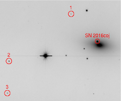
Figure 1.— KAIT unfiltered image showing the location of SN 2016coj. Three reference stars are also marked with circles.

KAIT performed photometric follow-up observations of SN 2016coj with nearly daily cadence after discovery. The data were reduced using our image-reduction pipeline (Ganeshalingam et al. 2010). We applied an image-subtraction procedure to remove host-galaxy light, and point-spread-function photometry was then obtained using DAOPHOT (Stetson 1987) from the IDL Astronomy User’s Library. The unfiltered instrumental magnitudes, which are found to be close to the $R$ band (Li et al. 2003), are calibrated to local SDSS standards (see Figure 1) transformed into Landolt $R$-band magnitudes. Here we publish our unfiltered photometry (Table 1). We have also obtained a filtered data sequence, but we are still awaiting high-quality galaxy template images in those bands.

Figure 2.— Left panels: Arbour’s image taken on May 23. Middle panels: KAIT unfiltered image taken on May 24. Right panels: KAIT unfiltered image taken on May 28. Upper panels show the original image and lower panels show the residual after subtraction; SN 2016coj is marked.

Interestingly, we find that SN 2016coj was detected in a KAIT prediscovery image taken at 04:30:35 on May 24 (see middle panels of Figure 2) with an unfiltered mag of $18.02\pm 0.22$, which means the SN had brightened $\sim 3.0$ mag in the following four days until it was discovered. In addition, an unfiltered prediscovery detection was obtained at 21:48:57 on May 23, 6.7 hr earlier than KAIT’s first detection, by R. Arbour with a 0.35 m $f/6$ Schmidt-Cassegrain reflector (see left panels of Figure 2). Using a template image taken on 2016 April 5, we performed the same subtraction and calibration methods as for the KAIT unfiltered images. We find a SN unfiltered brightness of $18.06\pm 0.42$ mag, consistent with KAIT’s first detection. A $\sim 5$ mag detection before peak magnitude, along with our analysis in the following section, confirms that SN 2016coj is one of the youngest SNe Ia ever detected.

Table 1Unfiltered Photometry of SN 2016coj

MJD	UT	Mag	Error	From
57520.2370	May 12.2370	$>$19.6	-	KAIT
57522.2513	May 14.2513	$>$19.4	-	KAIT
57524.2240	May 16.2240	$>$19.4	-	KAIT
57525.2479	May 17.2479	$>$19.3	-	KAIT
57527.2708	May 18.2708	$>$19.2	-	KAIT
57531.9092	May 23.9092	18.06	0.42	R. Arbour
57532.1877	May 24.1877	18.02	0.22	KAIT
57536.2694	May 28.2694	14.98	0.03	KAIT
57537.2196	May 29.2196	14.50	0.04	KAIT
57538.1827	May 30.1827	14.11	0.03	KAIT
57539.1814	May 31.1814	13.85	0.03	KAIT
57540.2518	June 01.2518	13.54	0.04	KAIT
57541.2022	June 02.2022	13.39	0.06	KAIT
57542.2075	June 03.2075	13.18	0.03	KAIT
57543.2120	June 04.2120	13.16	0.03	KAIT
57544.1995	June 05.1995	13.02	0.03	KAIT
57545.2245	June 06.2245	13.00	0.03	KAIT
57546.2200	June 07.2200	12.95	0.03	KAIT
57547.2051	June 08.2051	12.93	0.03	KAIT
57548.2197	June 09.2197	12.94	0.04	KAIT
57549.2162	June 10.2162	12.99	0.05	KAIT
57550.2638	June 11.2638	12.97	0.02	KAIT
57551.2201	June 12.2201	13.01	0.03	KAIT
57552.2516	June 13.2516	13.03	0.03	KAIT
57553.2115	June 14.2115	13.15	0.03	KAIT
57555.2189	June 16.2189	13.27	0.03	KAIT
57556.2284	June 17.2284	13.30	0.03	KAIT
57558.2110	June 19.2110	13.52	0.02	KAIT
57559.2229	June 20.2229	13.61	0.04	KAIT
57560.2189	June 21.2189	13.66	0.04	KAIT
57561.2097	June 22.2097	13.70	0.04	KAIT

Two classification spectra of SN 2016coj were obtained shortly ($\sim 3.7$ hr) after the SN was discovered ($\sim$ 5.0 days after the FFLT). The spectra were taken with the Kast double spectrograph (Miller & Stone 1993) on the Shane 3 m telescope at Lick Observatory and the FLOYDS robotic spectrograph on the Las Cumbres Observatory Global Telescope Network (LCOGT; Brown et al. 2013) 2.0 m Faulkes Telescope North on Haleakala, Hawaii. We obtained nearly daily spectra of SN 2016coj with different instruments including Kast, FLOYDS, the BFOSC spectrograph on the 2.16 m telescope at Xinglong station of NAOC (China), the Low Resolution Imaging Spectrometer (LRIS; Oke et al. 1995) on the 10 m Keck I telescope, and the Kitt Peak Ohio State Multi-Object Spectrograph (KOSMOS; Martini et al. 2014) on the KPNO Mayall 4 m telescope. Data were reduced following standard techniques for CCD processing and spectrum extraction using IRAF. The spectra were flux calibrated through observations of appropriate spectrophotometric standard stars. All Kast and LRIS spectra were taken at or near the parallactic angle (Filippenko 1982) to minimize differential light losses caused by atmospheric dispersion. Low-order polynomial fits to calibration-lamp spectra were used to calibrate the wavelength scale, and small adjustments derived from night-sky lines in the target frames were applied. Flux calibration and telluric-band removal were done with our own IDL routines; details are described by Silverman et al. (2012d).

We also obtained four epochs of Lick/Shane spectropolarimetry using the polarimetry mode of the Kast spectrograph on May 30, June 8, June 16, and July 6. The spectra were observed at each of four waveplate angles ($0^{\circ}$, $45^{\circ}$, $22.5^{\circ}$, and $67.5^{\circ}$) with several waveplate sequences coadded to improve the signal-to-noise ratio (S/N). Each night, both low- and high-polarization standard stars were also observed in order to calibrate the data. All of the spectropolarimetric reductions and calculations follow the method described by Mauerhan et al. (2015), and the polarimetric parameters are defined in the same manner (Stokes parameters $q$ and $u$, debiased polarization $P$, and sky position angle $\theta$).

In addition, we observed SN 2016coj on May 31, June 2, 4, and 6 with the 2.4 m Automated Planet Finder (APF) telescope at Lick Observatory. The APF hosts the Levy Spectrograph, a high-resolution optical echelle spectrograph with resolution $R$(5500 Å) $\approx$ 110,000 with a slit width of 1^′′ (Vogt et al. 2014). At each epoch we obtained three 1800 s spectra with the M decker (1$\farcs$0 wide, 8$\farcs$0 long to allow for background subtraction), reduced the data with a custom pipeline, and corrected for the redshift of the host galaxy ($z=0.004523$) and for the barycentric velocity ($\sim-15$ km s^-1). Because the apparent magnitude (peaking at $\sim 13$ mag) of SN 2016coj is a bit faint for APF, the S/N of our spectra was $\lesssim 10$ at best, significantly lower than obtained with APF spectra of the bright (peak $\sim 10$ mag), nearby SN Ia 2014J (Graham et al. 2015).

Figure 3.— KAIT unfiltered (red) light curve of SN 2016coj. The solid black line is the $t^{2.0}$ model fit to the red solid circles. The blue cross marks the earliest detection at $0.6\pm 0.5$ d after the fitted first light observed by R. Arbour. Red triangles show the KAIT upper limits before explosion.

3. Analysis and Results

3.1. Light Curve

Figure 3 shows our unfiltered light curve of SN 2016coj. In order to determine the first-light time $t_{0}$ (note that the SN may exhibit a “dark phase”), one can assume that the SN luminosity scales as the surface area of the expanding fireball, and therefore increases quadratically with time ($L\propto t^{2}$, commonly known as the $t^{2}$ model; Arnett 1982; Riess et al. 1999). The $t^{2}$ model fits well for several SNe Ia with early-time observations (e.g., SN 2011fe, Nugent et al. 2011; SN 2012ht, Yamanaka et al. 2014). Some studies also adopt a $t^{n}$ model ($n$ varies from $\sim 1.5$ to $\sim 3.0$; e.g., Conley et al. 2006; Ganeshalingam et al. 2011; Firth et al. 2015). Interestingly, Zheng et al. (2013, 2014) use a broken-power-law model to estimate the first-light time of SN 2013dy and SN 2014J. However, since our early-time photometric coverage of SN 2016coj is not as good as that of SN 2013dy and SN 2014J, we simply apply the $t^{2}$ model to fit the KAIT unfiltered data for the first few days (red solid circles in Figure 3); thereafter, the light curve starts deviating from the $t^{2}$ model. We also exclude Arbour’s unfiltered detection (blue cross), considering the different response curve compared to the KAIT unfiltered data: Arbour’s unfiltered band is closer to $V$ (see Botticella et al. 2009), while KAIT’s is closer to $R$ (see Li et al. 2003).

We find that the best $t^{2}$ model fit gives the first-light time to be MJD $=57531.33\pm 0.50$, around May 23.33. Here the uncertainty (not including the “dark phase”) is estimated by calculating the reduced $\chi^{2}$ ratio with the minimum reduced $\chi^{2}$ at 90% confidence level, when $t_{0}$ changes around the best-fitted value while all the other parameters are fixed with the best-fitted value. Note that the uncertainty does not include any systematic error caused by the $t^{2}$ model fitting. For example, if we include (or exclude) one data point before and after the dataset we used, the best-fit first-light time deviates $-0.4$ to 1.0 days from the above first-light time. Therefore, there could be a systematic error of up to 1.0 d from this method, which we did not include in the following analysis. Our results show that the first detection (from an image by R. Arbour) was merely $0.6\pm 0.5$ d after first light, or 0.9 d from KAIT’s first detection on May 24. This makes SN 2016coj one of the earliest detected SNe Ia — slightly later than SN 2013dy ($\sim 2.4$ hr after first light; Zheng et al. 2013) and SN 2011fe ($\sim 11.0$ hr after first light; Nugent et al. 2011), but similar to SN 2009ig ($\sim 17$ hr after first light; Foley et al. 2012).

Applying a low-order polynomial fit, we find that SN 2016coj reached a peak magnitude of $12.91\pm 0.03$ at MJD $=57547.31$ in KAIT unfiltered data. Although we do not present $B$-band data because no $B$-band template image is currently available, the fit allows us to determine the $B$-band peak time: MJD $=57547.35$, similar to the result with unfiltered data. This means SN 2016coj was discovered only 4.9 d after the fitted first light, or 11.1 d before maximum light.

The distance modulus of the host galaxy NGC 4125 is quite uncertain owing to different measurements given in NED. However, some of them are outdated, or adopted an inappropriate H₀ value. The one with the smallest uncertainty (and also the latest estimate) is $31.90\pm 0.14$ mag (Tully et al. 2013), which was based on H${}_{0}=74.4$ km s^-1 Mpc^-1, quite close to the current widely accepted value of H${}_{0}\approx 70$. We therefore adopt this distance for the following ananlysis. With $E(B-V)_{\textrm{MW}}=0.02$ mag (Schlafly et al. 2011) and very small (even negligible) host-galaxy extinction (see §3.2 and §3.5), this implies SN 2016coj has $M_{R}=-19.0\pm 0.2$ mag at peak brightness. Our preliminary measurement of $B$-band data, assuming the host background contamination is small, shows that the $B$-band peak is $\sim 13.1\pm 0.1$ mag and $\Delta m_{15}(B)=1.25\pm 0.12$ mag. This gives $M_{B}\approx-18.9\pm 0.2$ mag, but we expect $M_{B}\approx-19.1$ mag from the Phillips (1993) relation with the above value of $\Delta m_{15}(B)$; thus, SN 2016coj is a normal-brightness SN Ia. Its $\Delta m_{15}(B)=1.25\pm 0.12$ mag is also typical of normal SNe Ia (see also §3.3 for the spectral classification).

3.2. Optical Spectra

We obtained optical spectra of SN 2016coj nearly daily for a month (Fig. 4), sometimes obtaining multiple spectra in a given night.

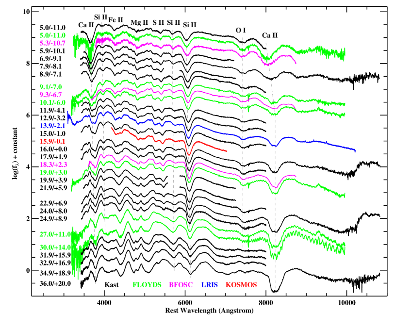
Figure 4.— Spectral sequence of SN 2016coj over the first month after discovery. Each spectrum is labeled with its age relative to both the fitted first light and to the $B$-band maximum light. Some major spectral features are labeled at the top. Spectra taken by different instruments are shown in different colors. Three Lick/Kast spectra have no coverage around 5500–5900 Å; those sections are left blank. Dashed lines are meant to help guide the eye when examining absorption features.

We first examine the Na I D absorption feature, which is often converted into reddening but with large scatter over the empirical relationship (Poznanski et al. 2011), in several of our high-S/N spectra. The absorption is not clearly detected at both the Na I D rest-frame wavelength and the redshifted wavelength of SN 2016coj. However, there appears to be a weak absorption feature consistent with the rest-frame Na I D wavelength. If real, this could be caused by a Milky Way component, which has $E(B-V)_{\textrm{MW}}=0.02$ mag according to Schlafly et al. (2011). Since we do not detect similar absorption at the redshifted wavelength of SN 2016coj, we can put an upper limit of $E(B-V)\lesssim 0.02$ mag of host-galaxy extinction. However, if the weak absorption feature is caused by noise instead of Milky Way gas, we can determine an upper limit on $E(B-V)$ through comparison with our spectra of SN 2013dy (Zheng et al. 2013), where we clearly detect the Na I D absorption with the same instrument setting. For SN 2013dy, the equivalent width ($W_{\lambda}$) is $\sim 0.5$ Å from both the Milky Way and host galaxy, giving $E(B-V)=0.15$ mag. Our similar-quality data on SN 2016coj should allow a detection of 1/3 (or less) of Na I D absorption if it exists, yielding an upper limit of $E(B-V)\lesssim 0.05$ mag of host-galaxy extinction. Lastly, we also estimate a $3\sigma$ upper limit on the $W_{\lambda}$ of an undetected feature in a spectrum using the equation presented by Leonard (2007): $W_{\lambda}(3\sigma)=3\Delta\lambda\ \Delta I\sqrt{W_{\rm line}/\Delta\lambda}\sqrt{1/B},$ where $\Delta\lambda$ is the spectral resolution element (in Å), $\Delta I$ is the 1$\sigma$ root-mean-square fluctuation of the flux around a normalized continuum level, $W_{\rm line}$ is the full-width at half-maximum intensity (FWHM) of the expected line feature, and $B$ is the number of bins per resolution element. For our high-S/N Kast spectra, we measure $\Delta\lambda\approx 4.0$ Å, $\Delta I\approx 0.015$, $W_{\rm line}\approx 12.0$ Å, and $B=1$, which gives $W_{\lambda}(3\sigma)\approx 0.3$ Å, and $E(B-V)\lesssim 0.09$ mag of host-galaxy extinction.

All of the above suggests that the host-galaxy extinction of SN 2016coj is likely to be very small, consistent with the nondetection of Na I D absorption in our high-resolution spectra (see §3.5). However, note that since the Na I D vs. extinction relation has large scatter, even a nondetection of Na I D does not fully exclude the possibility that there may be some dust along the SN line of sight.

The spectra show absorption features from ions typically seen in SNe Ia including Ca II, Si II, Fe II, Mg II, S II, and O I. We do not find a clear C II feature (e.g., Zheng et al. 2013), which is found in over one-fourth of all SNe Ia (e.g., Parrent et al. 2011; Thomas et al. 2011; Folatelli et al. 2012; Silverman et al. 2012b). Strong absorption features of Si II, including Si II $\lambda$4000, Si II $\lambda$5972, and Si II $\lambda$6355, are clearly seen in all spectra. The Si II $\lambda$5972 feature in SN 2016coj is quite strong relative to those in SN 2012cg and SN 2013dy, though it is relatively small if compared with a large SN Ia sample (see Silverman et al. 2012c).

We measure the individual line velocities from the minimum of the absorption features (see Silverman et al. 2012c, for details) and show them in Figure 6. The velocities all Si II features decrease from $\sim 13,000$–15,000 km s^-1 at discovery to $\sim 11,000$–13,000 km s^-1 around maximum light, and they continue to decrease thereafter.

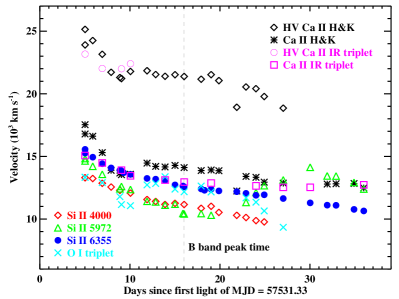
Figure 5.— The expansion velocity evolution of different lines measured from the spectra of SN 2016coj. The black dashed line marks the time of $B$-band maximum light.

In addition to the usual photospheric-velocity feature (PVF) of Ca II H&K, SN 2016coj exhibits a high-velocity feature (HVF; e.g., Mazzali et al. 2005; Maguire et al. 2012; Folatelli et al. 2013; Childress et al. 2014; Maguire et al. 2014; Silverman et al. 2015) in nearly all of the early-time spectra. This HVF appears to be detached from the rest of the photosphere, with a velocity of $\sim 25,000$ km s^-1 at discovery and slowing down to $\sim 20,000$ km s^-1 at $\sim 8$ d after the fitted first-light time. The HVF feature of Ca II H&K stays for a long time, being distinct until roughly age +11 d; thereafter, it is a high-velocity shoulder of the Ca II H&K absorption.

A Ca II near-infrared (NIR) triplet HVF is also found in the first few spectra that covered the wavelength range before maximum light, and the velocity of $\gtrsim 22,000$ km s^-1 is in good agreement with that of the Ca II H&K HVF at early times, though it is slightly smaller in the first-epoch spectrum. Such HVFs are seen in a few other well-observed SNe Ia, including SN 2005cf (Wang et al. 2009) and SN 2012fr (e.g., Maund et al. 2013; Childress et al. 2013; Zhang et al. 2014). However, in SN 2016coj, the Ca II NIR triplet HVF becomes weaker around peak brightness, and it completely disappears $\sim 8$ d later and thereafter. This is different from the Ca II H&K HVF, which is seen for a much longer time. It is not obvious why the HVF of the Ca II NIR triplet goes away after peak brightness while the HVF of Ca II H&K persists. One possibility is that the apparent HVF of Ca II H&K after peak could actually be Si II $\lambda$3858 (e.g., Foley 2013). In fact, it is possible that the early-time apparent HVF of Ca II H&K could be a mixture of Si II $\lambda$3858 (including both the HVF and PVF) plus the true HVF of Ca II H&K. If so, the velocity of the Ca II H&K HVF could be smaller than that shown in Figure 6, and thus more consistent with the velocity of the Ca II NIR triplet HVF, but this case is too complicated to verify.

One note about the O I triplet feature is that we adopted only one component in our fit. However, our early-time spectra before peak brightness reveal that the O I triplet has a double absorption profile. Following the Zhao et al. (2016) method to fit the O I triplet with both HVF and PVH (Zhao et al. also adopted a second, faster HVF, but that is not clear in SN 2016coj), we find an HVF O I triplet velocity of $\sim 16,000$ km s^-1 and a PVF O I triplet velocity of $\sim 12,000$ km s^-1. The HVF velocity is smaller than that of both Ca II H&K and the Ca II NIR triplet. If the HVF really exists in the O I triplet, it suggests that the oxygen in the outer layers is not completely burned (see Zhao et al. 2016).

The strong absorption of Si II $\lambda$6355 is commonly used to estimate the photospheric velocity. As shown in Figure 6, the Si II $\lambda$6355 velocity of SN 2016coj decreases rapidly from $\sim 15,500$ km s^-1 at discovery to $\sim 12,600$ km s^-1 around peak brightness, and then slowly decreases to $\sim 11,600$ km s^-1 at +11.0 d after peak. A velocity of $\sim 12,600$ km s^-1 at peak brightness is $\sim 1500$ km s^-1 higher than average in SNe Ia (e.g., Wang et al. 2013; $>2.5\sigma$ away from the mean of their SN Ia velocity distribution fitted with a Gaussian). Here, we compare the photospheric velocity measurement of SN 2016coj with the three well-observed SNe Ia 2009ig (Foley et al. 2012; Marion et al. 2013), 2012cg (Silverman et al. 2012a), and 2013dy (Zheng et al. 2013). Note that while both SN 2012cg and SN 2009ig have an HVF identified for Si II $\lambda$6355, we consider only the photospheric component.

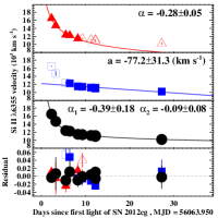
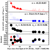
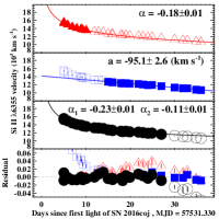
Figure 6.— Photospheric velocity (measured from the strong Si II $\lambda$6355 absorption) evolution of SN 2016coj (right panel), compared to those of the well-observed SN 2009ig (left panel), SN 2012cg (middle-left panel), and SN 2013dy (middle-right panel). For all SNe Ia, the top panels show the result of a power-law function fit to the early-time data, the middle-top panels display the result of a linear function fit to the later-time data, the middle-bottom panels give the result of a broken-power-law function fit to all the data, and the bottom panels show the residuals for each fit. Solid points are included in the fitting while open points are not.

Figure 6 displays the photospheric velocity evolution over time for the four SNe Ia. Overall, the photospheric velocity evolution is similar to the evolution seen in most SNe Ia (e.g., Benetti et al. 2005; Foley et al. 2011b; Silverman et al. 2012c): the velocity drops rapidly at early times (within the first week after explosion), and then slowly but steadily decreases thereafter. For each of these four SNe, we consequently try to fit the early-time velocities (typically within 10 d after first light) with a power-law function, $v=C_{1}t^{\prime\alpha}$, where $t^{\prime}$ is the time after first light ($t_{0}$); the results are shown in the top panel of Fig. 6 for each SN. This is very similar to the method Silverman et al. (2015, Fig. 12) adopted, but they used a natural exponential function to fit the velocities before +5 d after peak brightness and also obtained reasonable fitting results. In fact, Piro & Nakar (2013, Eq. 13) mathematically show that the photospheric velocity could decay as a power law at early times. For the later velocities (typically $>10$ d after first light), we then fit them with a linear function, $v=at^{\prime}+C_{2}$ (results shown in the middle-top panel); Silverman et al. (2012c, Fig. 5) also use the same method to fit their data around peak brightness. As seen in Figure 6, both the power-law function and the linear function can fit the corresponding data well, but only in their respective regimes — early-time data for the power-law function and later-time data for the linear function.

As with the early-time light-curve (Zheng et al. 2013, 2014), we find that a broken-power-law function is useful for fitting the photospheric velocity evolution; a low-index power-law function approximates the linear function found at late times. Specifically,

$$v=A\left(\frac{t^{\prime}}{t_{b}}\right)^{{\alpha}_{1}}\Big{[}1+\left(\frac{t^{\prime}}{t_{b}}\right)^{s({\alpha}_{1}-{\alpha}_{2})}\Big{]}^{-1/s},$$ (1)

where $v$ is the photospheric velocity, $A$ is a scaling constant, $t^{\prime}$ is the time after first light ($t_{0}$), $t_{b}$ is the break time, ${\alpha}_{1}$ and ${\alpha}_{2}$ are the two power-law indices before and after the break (respectively), and $s$ is a smoothing parameter. We apply this broken-power-law function to the entire dataset of photospheric velocities for all four SNe until about a month after the explosion. Our fitting results (we fixed $s$ to be $-10$) are listed in Table 2 and shown in the middle-bottom panels in Figure 6.

Table 2Photospheric Velocity Fitting Results

	$\alpha$	a	$\alpha_{1}$	$\alpha_{2}$	reduced $\chi^{2}$
SN	power law	lineara	broken power lawb
SN 2009ig	-0.16$\pm$0.04	-32$\pm$31	-0.20$\pm$0.14	0.03$\pm$0.23	0.04
SN 2012cg	-0.28$\pm$0.05	-77$\pm$32	-0.39$\pm$0.18	-0.09$\pm$0.08	0.04
SN 2013dy	-0.22$\pm$0.03	-54$\pm$32	-0.34$\pm$0.16	-0.11$\pm$0.06	0.14
SN 2016coj	-0.18$\pm$0.01	-95$\pm$3	-0.23$\pm$0.01	-0.11$\pm$0.01	1.72

The power-law indices from both the power-law fitting ($\alpha$) and broken-powerlaw fitting ($\alpha_{1}$) at early times are consistent with the value of $-0.22$ adopted by Piro & Nakar (2014) when fitting three SNe Ia (SNe 2009ig, 2011fe, and 2012cg), and are also the value adopted by Shappee et al. (2016) when fitting ASASSN-14lp. The index from the broken power law ($\alpha_{1}$) is slightly steeper than that from the power law ($\alpha$). At late times (around maximum light) with linear fitting, the rate of velocity decrease from the fitting is slightly larger than the average rate of $-38$ km s^-1 d^-1 found by Silverman et al. (2012c) for a large sample of SNe Ia.

Overall, the broken-power-law function can fit the photospheric velocity evolution well for all four SNe until a month after explosion (see the small residuals at the bottom panel of Figure 6 and the reduced $\chi^{2}$ given in Table 2). This function also has the potential to fit the photospheric velocity evolution of most other SNe Ia as well, given that most SNe Ia have very similar velocity evolution (e.g., Silverman et al. 2012b, 2012c). High-cadence spectroscopy is required to verify this, especially at early times. However, currently it remains unclear whether there is a good physical explanation behind the fitting; Piro & Nakar (2013) show that the photospheric velocity could decay as a power law at early times, but our broken-power-law function fitting extends to a much later time.

3.3. Classification

We use the SuperNova IDentification code (SNID; Blondin & Tonry 2007) to spectroscopically classify SN 2016coj. For nearly all of the spectra presented here, we find that SN 2016coj is spectroscopically similar to many normal SNe Ia. Compared to SN 1992A ($M_{B}=-18.79$ mag and $\Delta m_{15}(B)=1.47$ mag; Della Valle et al. 1998) and SN 2002er ($M_{B}=-19.35$ mag and $\Delta m_{15}(B)=1.33$ mag; Pignata et al. 2004), for example, SN 2016coj has similar spectra, absolute magnitude, and $\Delta m_{15}(B)$. Another spectroscopic comparison is the so-called Si II ratio, $\Re$(Si II) (the ratio of Si II $\lambda$5972 to Si II $\lambda$6355), defined by Nugent et al. (1995) using the depths of spectral features and later by Hachinger et al. (2006) using their pseudo-equivalent widths. Hachinger et al. (2006) found a good correlation between the $\Re$(Si II) and $\Delta m_{15}(B)$ (see their Figure 13). We measure SN 2016coj to have $\Re$(Si II) $=0.11\pm 0.4$, with $\Delta m_{15}(B)=1.25$ mag, placing SN 2016coj in the normal SN Ia region in Figure 13 of Hachinger et al. (2006), very close to SN 2002er. Thus, we conclude that SN 2016coj is a spectroscopically normal SN Ia, consistent with the photometric analysis given in §3.1.

3.4. Spectropolarimetry

Figure 7.— Four epochs of spectropolarimetry of SN 2016coj. Top panel: observed total-flux spectrum, color coded for each epoch. Middle panel: Debiased polarization ($P$), with several major features labeled. Bottom panel: Position angle ($\theta$) for the corresponding epochs. $\theta$ is underdetermined where $P/\sigma P>1.5$; those points are omitted.

3.4.1 Interstellar and Instrumental Polarization

The interstellar polarization (ISP) appears to be low in the direction of SN 2016coj. Indeed, the estimated value of $E(B-V)=0.02$ mag indicates that the extinction from the Milky Way and host galaxy are not substantial; a small contribution from ISP is thus to be expected. According to Serkowski et al. (1975), an upper limit to the ISP is given by $9\times E(B-V)$, which implies $P_{\rm ISP}<0.18\%$ for SN 2016coj. To obtain a direct estimate of the Galactic component of ISP, we observed three Galactic stars in the vicinity of the SN position: HD 104436 (A3 V), HD 106998 (A5 V), and HD 108907 (M3 III). We measure respective $V$-band polarization and $\theta$ values of $P=(0.12\%,0.09\%,0.09\%)$ and $\theta=(36^{\circ},34^{\circ},30^{\circ})$. Under the reasonable assumption of low intrinsic polarization for these stars, the resulting average values of $P\approx 0.1$%, $\theta\approx 33^{\circ}$ confirm the low Galactic polarization. Furthermore, the lack of Na I D absorption lines in our low- and high-resolution spectra (see §3.2 and §3.5) indicates low extinction from the early-type host galaxy, and thus implies that the host ISP is probably even lower than the small Galactic value.

The instrumental polarization of the Kast instrument is also low. Measurements of the low-polarization standard star BD$+$33 2642 at each epoch indicate an average $V$-band polarization of $\sim 0.15$%, with a standard deviation of 0.05% between all four epochs; the average value is consistent with that reported by Schmidt et al. (1992) for this star, which indicates that the low level is intrinsic to the source and that Kast contributes an insignificant amount of instrumental polarization to the measurements. The standard deviation is near the systematic uncertainty level we typically experience using the spectropolarimetry mode of Kast. Our observations therefore constrain the average instrumental polarization to $<0.05\%$. Based on the low values of ISP and instrumental polarization, we move forward without attempting to subtract their minor contributions from the data.

3.4.2 Intrinsic Polarization

Our spectropolarimetry results are shown in Figure 7 and the integrated broadband measurements are listed in Table 3. On day 6.9, the source exhibits weak polarization in the continuum at a level of $\sim 0.3$%, integrated over the wavelength range 6700–7150 Å. This is consistent with the weak levels of continuum polarization that are typically associated with SNe Ia (Wang & Wheeler 2008), although we note that some fraction of the polarization, perhaps half, could potentially be contributed by ISP. Strong polarization is exhibited across prominent line features, particularly Si II $\lambda$6355 and the Ca II NIR triplet, at levels of $\sim 0.9$% and $\sim 0.6$%, respectively. The Ca II polarization feature appears to exhibit two peaks, perhaps associated with the high- and low-velocity components. The position angles across the polarized line features, particularly Si II, are close to that of the continuum, which suggests an axisymmetric configuration for the SN.

By day 16.0, the continuum polarization is consistent with having no change relative to day 6.9, while Si II has increased in strength slightly to peak at this epoch. A Gaussian fit to the Si II feature indicates a line polarization of $0.9\pm 0.1\%$ with respect to the continuum level. For Ca II polarization, the enhancement of the high-velocity component from day 6.9 has disappeared and the peak of the lower-velocity component has increased by $\sim 0.3$%.

By day 24.0, the continuum and Si II line polarization appears to have dropped substantially for wavelengths shortward of 7000 Å, with no significant change apparent at longer wavelengths; polarization in the continuum region is undetected at this epoch. If real, such a continuum polarization drop roughly one week after peak would be reminiscent of the evolution of SN 2001el (Wang et al. 2003). However, by day 44.0 the continuum polarization appears to have regained the strength exhibited on day 16.0 and earlier. Si II has restrengthened as well, while declining in radial velocity along with the minimum of the weakening absorption profile. Based on this unexpected restrengthening, we exercise caution regarding the temporarily weakened polarization on day 24.0, as we are concerned that this could be the result of a systematic error. The drop in polarization appears to have only affected the Stokes $q$ parameter (derived from exposures with polarimeter waveplate angles at 0^∘ and 45^∘). Each of our three $q$ sequences of the SN are consistent, and we see no such change in the $q$ parameter of our standard-star observations from the same night. Thus, if the change on day 24.0 is the result of systematic error (e.g., some unknown temporary source of instrumental polarization above our typical limit of $<0.05$%), then it must have occurred over an hourly timescale. Alternatively, a subsequent rise in continuum polarization on day 44.0 could result from the appearance of weak line features in the our chosen continuum region (6700–7150 Å), but in this case we would not expect the simultaneous rise in the Si II feature. As a final possibility, the temporary influence of a separate light-echo component, possibly associated with dust in the host ISM, could result in the observed fluctuation; this possibility has the advantage of accounting for the brief change in the continuum and line polarization simultaneously, and it would also explain why the reddest wavelengths are not significantly affected.

Overall, the spectropolarimetric character of SN 2016coj is consistent with the trends exhibited by “normal” SNe Ia. For example, Maund et al. (2010) reported a correlation between the polarization of the Si II $\lambda$6355 feature, measured near or before peak luminosity, and the radial-velocity decline rate of the absorption minimum (also see Leonard et al. 2006), physically interpreted as evidence for a single geometric configuration for normal SNe Ia. At peak brightness on day 16.0, the line polarization of $0.9\pm 0.1\%$ combined with our measured value of $-95$ km s^-1 day^-1 for the velocity evolution, shows that SN 2016coj falls where expected on the correlated distribution of SNe Ia reported by Maund et al. (2010), and within the range of high-velocity explosions.

Table 3Polarization of SN 2016coj

Epoch	$P_{V}\tablenotemark{a}$(%)	$\theta_{V}$(deg)	$P_{\textrm{\tiny{cont}}}$	$\theta_{\textrm{\tiny{cont}}}$(deg)
6.9	0.27(0.01)	54.3(0.8)	0.51(0.01)	55.4(0.9)
16.0	0.20(0.01)	52.6(0.8)	0.38(0.01)	53.4(0.8)
24.0	0.16(0.01)	39.2(1.6)	0.06(0.02)	09.0(4.3)
44.0	0.39(0.04)	41.0(1.3)	0.28(0.03)	30.0(2.2)

3.5. High-Resolution Spectra

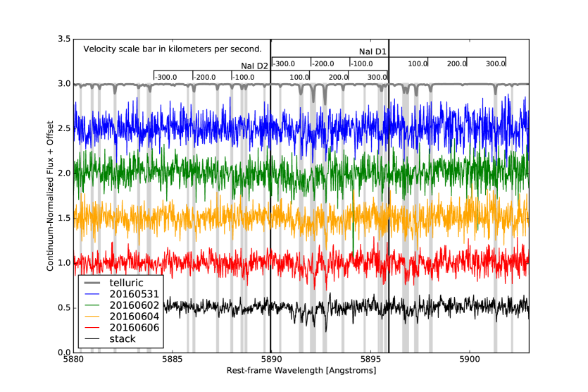
Figure 8.— High-resolution spectra of SN 2016coj in the region of Na I D absorption from the APF obtained at four epochs (2016-05-31, blue; 2016-06-02, green; 2016-06-04, orange; 2016-06-06, red). The bottom (black) shows the stacked spectrum from the data of these epochs. A mean barycentric velocity of $\sim 15$ km s^-1 has been applied for all epochs of SN 2016coj spectra. The atmospheric absorption lines are shown in gray, which has been redshifted into the frame of SN 2016coj. The most significant features are highlighted with vertical bars in order to identify their presence in the spectra of SN 2016coj. A rest-frame velocity scale bar is provided for each Na I D feature along the top of the plot.

We examine the APF high-resolution spectra for narrow absorption features, such as those that were identified in APF spectra of SN 2014J (Graham et al. 2015). We began spectral monitoring with the APF based on an early classification and the assumption of a host-galaxy distance smaller than that adopted here. The object’s peak apparent brightness ended up being $\sim 3$ mag fainter than that of SN 2014J, and fainter than the projected minimum we typically require for triggering the APF. For this reason, the S/N of our SN 2016coj APF spectra is quite low. Instead of ceasing our APF monitoring we obtained multiple observations over several nights in order to stack our spectra, but ultimately we do not identify any absorption features of Na I D $\lambda\lambda$5889.95, 5895.92, Ca II H&K $\lambda\lambda$3933.7, 3968.5, K I $\lambda\lambda$7664.90, 7698.96, H$\alpha$ $\lambda$6562.801, H$\beta$ $\lambda$4861.363, or the diffuse interstellar bands ($\lambda\approx 5780$, 5797, 6196, 6283, 6613 Å).

Since the Na I D feature is most useful for constraining the presence of circumstellar material and line-of-sight host-galaxy dust extinction, and owing to grating blaze is in a region of relatively higher S/N ($\sim 10$), we estimate an upper limit on its $W_{\lambda}$ in the following way. The flux of the continuum-normalized stacked APF spectra in the region of Na I D, shown in black in Figure 8, has a standard deviation of $\sigma\approx 0.038$. As an upper limit on the depth of an absorption feature that we could have detected, we use $3\sigma\approx 0.11$. Our instrumental configuration for the Levy spectrograph results in a spectral resolution of $\Delta\lambda\approx 0.03$ Å, from which we estimate that the minimum FWHM of a detected feature is $3\Delta\lambda\approx 0.1$ Å. Assuming a Gaussian profile for this hypothetical absorption, we constrain the Na I D feature to have $W_{\lambda}\lesssim 0.56$ Å. Based on Figure 9 of Phillips et al. (2013), this puts an upper limit on host-galaxy extinction of $A_{V}\lesssim 0.2$ mag (with $E(B-V)=0.07$ mag assuming $R_{V}=3.1$). Although this is a rather large upper limit, it is consistent with the small host-galaxy extinction constrained from our low-resolution spectra (see §3.2) and also with the low extinction expected given the early type of the host, NGC 4125.

4. Conclusions

In this paper we have presented optical photometric, low- and high-resolution spectroscopic, and spectropolarimetric observations of SN 2016coj, one of the youngest discovered and best-observed SNe Ia. Our clear-band light curve shows that our first detection is merely $0.6\pm 0.5$ d after the fitted time of first light, making it one of the earliest detected SNe Ia. We estimate that SN 2016coj took $\sim 16.0$ d after the fitted first-light time to reach $B$-band maximum. Its maximum brightness has a normal luminosity, $B=-18.9\pm 0.2$ mag. An estimated $\Delta m_{15}(B)$ value of 1.25 mag along with spectral information support its normal SN Ia classification. In the well-observed low-resolution spectral sequence, we identify a high-velocity feature from both Ca II H&K and the Ca II NIR triplet, and also possibly from the O I triplet. SN 2016coj has a Si II $\lambda$6355 velocity of $\sim 12,600$ km s^-1 at peak brightness, $\sim\,1500$ km s^-1 higher than that of typical SNe Ia. We find that the Si II $\lambda$6355 velocity decreases rapidly during the first few days and then slowly decreases after peak brightness, very similar to that of other SNe Ia. A broken-power-law function can well fit the Si II $\lambda$6355 velocity for up to about a month after first light. We estimate there to be very small host-galaxy extinction based on the lack of Na I D lines from the host galaxy in our low- and high-resolution spectra. Our four epochs of spectropolarimetry show that SN 2016coj exhibits weak polarization in the continuum, but the Si II line polarization is quite strong ($\sim 0.9\pm 0.1$%) at peak brightness.

References

- (1) Blanchard, P., Zheng, W., Cenko, S. B., et al. 2013, CBET, 3422
- (2) Benetti, S., et al. 2005, ApJ, 623, 1011
- Blondin & Tonry (2007) Blondin, S., & Tonry, J. L. 2007, ApJ, 666, 1024
- (4) Blondin, S., et al. 2009, ApJ, 693, 207
- (5) Bloom, J., et al. 2012, ApJL, 744, L17
- (6) Botticella, M. T., et al. 2009, 398, 1041
- (7) Brown, T. M., et al. 2013, PASP, 125, 1031
- (8) Casper, C., et al. 2013, CBET, 3700
- (9) Cao, Y., et al. 2015, Nature, 521, 328
- (10) Cao, Y., et al. 2016, arXiv:1606.05655
- (11) Cenko, S. B., et al. 2012, CBET, 3199
- (12) Childress, M., et al. 2013, ApJ, 770, 29
- (13) Childress, M., et al. 2014, MNRAS, 437, 338
- (14) Conley, A., et al. 2006, ApJ, 132, 1707
- (15) de Vaucouleurs, G., de Vaucouleurs, A., Corwin, H. G., Jr., Buta, R. J., Paturel, G., & Fouqué, P. 1991, RC3.9, “Third Reference Catalogue of Bright Galaxies,” version 3.9 (New York: Springer)
- (16) Della Valle, M. 1998, MNRAS, 299, 267
- (17) Dhungana, G., et al. 2016, ApJ, 822, 6
- (18) Filippenko, A. V. 1982, PASP, 94, 715
- (19) Filippenko, A. V. 1997, ARA&A, 35, 309
- (20) Filippenko, A. V. 2005, in 1604–2004, Supernovae as Cosmological Lighthouses, ed. M. Turatto, et al. (San Francisco: ASP), 87
- Filippenko et al. (2001) Filippenko, A. V., Li, W. D., Treffers, R. R., & Modjaz, M. 2001, in Small-Telescope Astronomy on Global Scales., ed. B. Paczyński, W. P. Chen, & C. Lemme (San Francisco: ASP), 121
- (22) Firth, R. E., et al. 2015, MNRAS, 446, 3895
- (23) Folatelli, G., et al. 2012, ApJ, 745, 74
- (24) Folatelli, G., et al. 2013, ApJ, 773, 53
- (25) Foley, R. J., et al. 2011a, ApJ, 729, 55
- (26) Foley, R. J., et al. 2011b, ApJ, 742, 89
- Foley et al. (2012) Foley, R. J., et al. 2012, ApJ, 744, 38
- (28) Foley, R. J. 2013, MNRAS, 435, 273
- Ganeshalingam et al. (2010) Ganeshalingam, M., et al. 2010, ApJS, 190, 418
- (30) Ganeshalingam, M., Li, W., & Filippenko, A. V. 2011, MNRAS, 416, 2607
- (31) Goobar, A., et al. 2014, 784, L12
- (32) Graham, M., et al. 2015, 801, 136
- (33) Hachinger, S. et al. 2006, MNRAS, 370, 299
- (34) Hachisu, I., et al. 1996, ApJL, 470, L97
- (35) Hayakawa, K., et al. 2013, CBET, 3706
- (36) Hillebrandt, W., & Niemeyer, J. C. 2000, ARA&A, 38, 191
- (37) Höflich, P. 1991, A&A, 246, 481
- (38) Hoyle, F., & Fowler, W. A. 1960, ApJ, 132, 565
- (39) Humphrey, P. J. 2009, ApJ, 690, 512
- (40) Hsiao, E. Y., et al. 2015, A&A, 578, 9
- (41) Hughes, A., et al. 2015, CBET, 4169
- (42) Iben, I., Jr., & Tutukov, A. V. 1984, ApJS, 54, 335
- (43) Kandrashoff, M., et al. CBET, 3121
- (44) Kasen, D., et al. 2003, ApJ, 593, 788
- Kasen (2010) Kasen, D. 2010, ApJ, 708, 1025
- (46) Kim, M., et al. 2013a, CBET, 3678
- (47) Kim, H., et al. 2013b, CBET, 3743
- (48) Kim, M., Zheng, W., Li, W., & Filippenko, A. V. 2014a, CBET, 3777
- (49) Kim, H., et al. 2014b, CBET, 3942
- (50) Kumar, S., et al. 2014, CBET, 4165
- (51) Leaman, J., Li, W., Chornock, R., & Filippenko, A. V. 2011, MNRAS, 412, 1419
- (52) Leonard, D. 2007, ApJ, 670, 1275
- (53) Li, W., et al. 2003, PASP, 115, 844
- (54) Li, W., et al. 2011, Nature, 480, 348
- (55) Maguire, K., et al. 2012, MNRAS, 426, 2359
- (56) Maguire, K., et al. 2014, MNRAS, 444, 3258
- (57) Martini, P., et al. 2014, SPIE, 9147, 91470Z-11
- (58) Mauerhan J. C., et al. 2015, MNRAS, 453, 4467
- Maund et al. (2010) Maund, J. R., Höflich, P., Patat, F., et al. 2010, ApJL, 725, L167
- (60) Maund, J. R., et al. 2013, MNRAS, 433, L20
- (61) Mazzali, P. A., et al. 2005, ApJ, 623, L37
- (62) Meng, X., et al. 2009, MNRAS, 395, 2103
- Miller & Stone (1993) Miller, J. S., & Stone, R. P. S. 1993, Lick Obs. Tech. Rep. 66 (Santa Cruz: Lick Obs.)
- (64) Nugent, P., et al. 1995, ApJ, 455, L147
- Nugent et al. (2011) Nugent, P. E., et al. 2011, Nature, 480, 344
- (66) Oke, J. B., et al. PASP, 107, 375
- (67) Pakmor, R., et al. 2012, ApJL, 747, L10
- (68) Parrent, J. T., et al. 2011, ApJ, 732, 30
- (69) Patat, F., et al. 2007, Science, 317, 924
- Perlmutter et al. (1999) Perlmutter, S., et al. 1999, ApJ, 517, 565
- (71) Pignata, G., et al. 2004, MNRAS, 355, 178
- (72) Piro, A., & Morozova, V. S. 2016, ApJ, 826, 96
- (73) Piro, A., & Nakar, E. 2013, ApJ, 769, 67
- (74) Piro, A., & Nakar, E. 2014, ApJ, 784, 85
- Poznanski et al. (2011) Poznanski, D., Ganeshalingam, M., Silverman, J. M., & Filippenko, A. V. 2011, MNRAS, 415, L81
- (76) Rabinak, I., Livne, E., & Waxman, E. 2012, ApJ, 757
- Riess et al. (1998) Riess, A. G., et al. 1998, AJ, 116, 1009
- (78) Rópke, F. K., et al. 2012, ApJL, 750, L19
- (79) Ross, T. W., et al. 2015, CBET, 4125
- (80) Schlafly, E., et al. 2011, ApJ, 737, 103
- Schmidt et al. (1992) Schmidt, G. D., Elston, R., & Lupie, O. L. 1992, AJ, 104, 1563
- Serkowski et al. (1975) Serkowski, K., Mathewson, D. S., & Ford, V. L. 1975, ApJ, 196, 261
- (83) Shappee, B. J., et al. 2016, ApJ, 826, 144
- (84) Shivvers, I., et al. 2016, MNRAS, 461, 3057
- Silverman et al. (2012a) Silverman, J. M., et al. 2012a, ApJ, 756, L7
- Silverman et al. (2012b) Silverman, J. M., et al. 2012b, MNRAS, 425, 1917
- Silverman et al. (2012c) Silverman, J. M., et al. 2012c, MNRAS, 425, 1819
- (88) Silverman, J. M., et al. 2012d, MNRAS, 425, 1789
- (89) Silverman, J. M., et al. 2015, MNRAS, 451, 1973
- (90) Simon, J. D., et al. 2009, ApJ, 702, 1157
- (91) Stegman, S., Zheng, W., & Filippenko, A. V. 2014a, CBET, 4124
- (92) Stegman, S., Zheng, W., & Filippenko, A. V. 2014b, CBET, 4128
- (93) Sternberg, A., et al. 2014, MNRAS, 443, 1849
- (94) Thomas, R. C., et al. 2011, ApJ, 743, 27
- (95) Vogt, S., et al. 2014, PASP, 126, 359
- (96) Wang, L., et al. 1997, ApJ, 476, L27
- (97) Wang, L., et al. 2003, ApJ, 591, 1110
- (98) Wang, L., et al. 2007, Science, 315, 212
- Wang & Wheeler (2008) Wang, L., & Wheeler, J. C. 2008, ARA&A, 46, 433
- (100) Wang, X., et al. 2008, ApJ, 675, 626
- (101) Wang, X., et al. 2009, ApJ, 697, 380
- (102) Wang, X., et al. 2013, Science, 340, 170
- (103) Webbink, R. F. 1984, ApJ, 277, 355
- (104) Wilson, C. D., et al. 2013, ApJ, 776, 30
- (105) Yamanaka, M., et al. 2014, ApJ, 782, L35
- (106) Zhang, J., et al. 2014, AJ, 148, 1
- (107) Zhao, X. L., Maeda, K., Wang, X., et al. 2016, ApJ, 826, 211
- (108) Zheng, W., et al. 2013, ApJ, 778, L15
- (109) Zheng, W., et al. 2014, ApJ, 783, L24
- (110) Zheng, W., et al. 2016, ATel, 9095