Pulsar Timing Array Based Search for Supermassive Black Hole Binaries
in the Square Kilometer Array Era

Abstract

The advent of next generation radio telescope facilities, such as the Square Kilometer Array (SKA), will usher in an era where a Pulsar Timing Array (PTA) based search for gravitational waves (GWs) will be able to use hundreds of well timed millisecond pulsars rather than the few dozens in existing PTAs. A realistic assessment of the performance of such an extremely large PTA must take into account the data analysis challenge posed by an exponential increase in the parameter space volume due to the large number of so-called pulsar phase parameters. We address this problem and present such an assessment for isolated supermassive black hole binary (SMBHB) searches using a SKA era PTA containing $10^{3}$ pulsars. We find that an all-sky search will be able to confidently detect non-evolving sources with redshifted chirp mass of $10^{10}$ $M_{\odot}$ out to a redshift of about $28$ (corresponding to a rest-frame chirp mass of $3.4\times 10^{8}$ $M_{\odot}$). We discuss the important implications that the large distance reach of a SKA era PTA has on GW observations from optically identified SMBHB candidates. If no SMBHB detections occur, a highly unlikely scenario in the light of our results, the sky-averaged upper limit on strain amplitude will be improved by about three orders of magnitude over existing limits.

Introduction –

Several major efforts are progressing in parallel to open the gravitational wave (GW) window in astronomy across a wide range of frequencies. Success has been achieved in the high-frequency band ($\sim 10-1000$ Hz) with the landmark detection of signals from two binary black hole mergers by the Advanced Laser Interferometer Gravitational-Wave Observatory (aLIGO) (Abbott et al., 2016, 2016). Space-based detectors (Seoane et al., 2013; Sato et al., 2009; Luo et al., 2016), for scanning the $\sim 10^{-4}-1$ Hz band are in various stages of planning. Sensitivities of Pulsar Timing Array (PTA) based GW searches in the $\sim 10^{-9}-10^{-6}$ Hz band continue to improve Shannon et al. (2015); Lentati et al. (2015); Arzoumanian et al. (2016); Verbiest et al. (2016); Arzoumanian et al. (2014); Zhu et al. (2014); Babak et al. (2016).

PTA based GW astronomy will experience a sea change when next generation radio telescopes with larger collecting areas and better backend systems, such as FAST (Hobbs et al., 2014) and SKA (Smits et al., 2009), start observations. Simulations based on pulsar population models predict that up to 14000 canonical and 6000 millisecond pulsars (MSPs) can be discovered by SKA (Smits et al., 2009). Due to their high intrinsic rotational stability, combined with the improved sensitivity of SKA, a timing uncertainty of $<100$ ns Kramer et al. (2004); Manchester (2010) is likely for a substantial fraction of the MSPs.

The most promising class of GW sources for PTAs is that of Supermassive Black Hole Binaries (SMBHBs). While the number of optically identified SMBHB candidates now ranges in the hundreds Tsalmantza et al. (2011); Eracleous et al. (2012); Graham et al. (2015a); Charisi et al. (2016), the only unambiguous confirmation of the true nature of a candidate is its GW signal. If the constraints (Shannon et al., 2015) on models of the unresolved SMBHB population (Sesana et al., 2009) continue to improve in the absence of a detection of the associated stochastic signal – implying a sparser distribution of sources – the search for isolated sources becomes increasingly important.

We carry out a quantitative assessment of the performance one can expect for isolated SMBHB searches with an extremely large SKA era PTA containing $10^{3}$ pulsars. In order to make the assessment realistic, the exponential growth in the volume of the parameter space defining a GW signal must be taken into account. This happens because, as explained later, every pulsar in the array introduces a so-called pulsar phase parameter whose value is not known a priori. This problem is addressed in our analysis by using the algorithm proposed in Wang et al. (2015).

Preliminaries –

Let $d^{I}(t)$ denote the timing residual from the $I^{\rm th}$ pulsar, obtained by subtracting a fiducial timing model from the recorded pulse arrival times. The data from an $N$ pulsar PTA can be expressed as (Zhu et al., 2016),

$$\textbf{d}(t) = \textbf{A}\Delta\textbf{h}(t)+\textbf{n}(t)\;.$$ (1)

Here, $\textbf{d}(t)$ is the column vector whose $I^{\rm th}$ element is $d^{I}(t)$, and $\textbf{n}(t)$ is the corresponding column vector of noise in the observations. The $I^{\rm th}$ row of the $N$-by-2 response matrix A is comprised of the antenna pattern functions $F^{I}_{+}(\alpha,\delta)$ and $F^{I}_{\times}(\alpha,\delta)$ (their functional forms can be found in Wang et al. (2014)), with $\alpha$ and $\delta$ being the Right Ascension (RA) and Declination (DEC) of the GW source. $\Delta\textbf{h}(t)=(\Delta h_{+}(t),\Delta h_{\times}(t))^{T}$,

$$\Delta h_{+,\times}(t) = h_{+,\times}(t)-h_{+,\times}(t-\tau_{I}(\alpha,\delta))\,.$$ (2)

The last term in Eq. 2 is called the pulsar term. The time delay $\tau_{I}(\alpha,\delta)$ depends on the Earth-pulsar distance and the direction of the source relative to the line of sight to the pulsar.

The condition number of A, shown in Fig. 1, determines the degree of ill-posedness inherent in the inverse problem (Engl and Neubauer, 1996) of estimating signal parameters from the data.

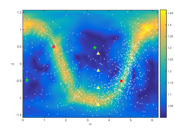
Figure 1: The condition number of the response matrix A as a function of RA ($\alpha$) and DEC ($\delta$), both expressed in radians. The dots show the locations of the MSPs constituting the simulated SKA era PTA used in this paper. The stars show the Galactic poles (North on top) and the squares show the Galactic Center (right) and anti-center (left). From top to bottom, the triangles denote the four source locations A, B, C, and D respectively that are used in the simulations. The condition numbers corresponding to these locations in the same order are: 1.0139, 1.0486, 1.1832, and 1.3159.

Simulated SKA era PTA –

We construct a realistic SKA era PTA using the simulated pulsar catalog in (Smits et al., 2009) and selecting $10^{3}$ MSPs within 3 kpc from us. Fig. 1 shows the locations of the simulated MSPs.

We generate data realizations using a uniform cadence for simplicity. It is set to two weeks, in order to match the typical cadence used in current PTAs. The span of the simulated timing residuals is 5 years. Noise realizations are drawn from an i.i.d. $\mathcal{N}(0,\sigma^{2})$ (zero mean white Gaussian noise) process, with $\sigma=100$ ns for all pulsars. The higher observational frequency band of SKA may also improve data quality by mitigating the problem of red noise Shannon et al. (2015).

Optimal Signal to Noise Ratio –

It is convenient to characterize a PTA using its network signal-to-noise ratio (SNR), $\rho$, defined as

$$\rho = \left[\sum_{I=1}^{N}\rho_{I}^{2}\right]^{1/2}\;,$$ (3)

$$\rho_{I} = \|F_{+}^{I}(\alpha,\delta)\Delta h_{+}+F_{\times}^{I}(\alpha,\delta)\Delta h_{\times}\|/\sigma_{I}\;.$$ (4)

Here, $\rho_{I}$ is the individual optimal SNR for the $I^{\rm th}$ pulsar, $\sigma_{I}=\sigma$ in our simulations, and $\|v\|^{2}=\sum_{i=1}^{k}v_{i}^{2}$ for $v\in\mathbb{R}^{k}$.

Fig. 2 shows the cumulative network SNR for a representative SMBHB system when the $\rho_{I}$ are arranged in descending order. It can be seen that a substantial fraction of pulsars must be included in order to avoid a significant loss of network SNR. Almost independently of the source location, contributions from $>200$ pulsars are needed to reach 90% of the total SNR. Taking only the top 20 pulsars, one gets less than 40% of the total SNR. Non-uniformly distributed noise levels ($\sigma_{I}$) in a real PTA will enhance the location dependence of the required fraction of pulsars but, qualitatively, give the same result.

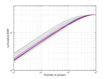
Figure 2: Cumulative network SNR for a uniformly spaced 6-by-6 grid of source locations (grey) and the four locations, A (blue), B (black), C (red), and D (magenta), used in the simulations. The total network SNR, $\rho$, is $30$ for this plot. The curve for any other $\rho$ can be obtained by using an overall scale factor of $\rho/30$.

It should be noted that while the metric $\rho$ is simple to compute, it pertains to the best-case scenario for a search where the GW signal parameters are known a priori. In reality, detection requires the global maximum, over all the signal parameters, of the joint log-likelihood function of the full data from a PTA. The resulting effect of the parameter space volume on the false alarm probability of the detection statistic is not accounted for in $\rho$.

Pulsar phase parameters –

For the large fraction of SMBHB sources that are expected to evolve slowly Rosado et al. (2015), $h_{+,\times}(t)$ is approximately monochromatic. The time delay $\tau_{I}(\alpha,\delta)$ (c.f. Eq 2) then transforms into a fixed phase offset, $\varphi_{I}$, called the pulsar phase parameter. Uncertainty in our knowledge of the Earth-pulsar distance makes $\varphi_{I}$ an a priori unknown quantity even if $\alpha$ and $\delta$ are known. Hence, every pulsar in a PTA contributes a new parameter to the joint log-likelihood. For a SKA era PTA, this leads to an infeasible optimization problem over hundreds of unknown parameters since, as discussed earlier, the bulk of the pulsars must be included in a search.

A solution to the pulsar phase problem is provided by a judicious choice of the parameters that are maximized over (semi-)analytically in the optimization process. Choosing the pulsar phase parameters as this subset Wang et al. (2014) leads to the MaxPhase algorithm (Wang et al., 2015). The remaining optimization, involving a fixed 7-dimensional search space, is carried out using Particle Swarm Optimization (PSO) Eberhart and Kennedy (1995); Wang and Mohanty (2010); Wang et al. (2014). (The PSO algorithm used here is slightly modified to improve performance for angular variables.) The applicability of the alternative approach of numerically optimizing over the pulsar phase parameters Zhu et al. (2016) has not been established for $\gtrsim 30$ pulsars. A method Taylor et al. (2014) that obtains a 7 dimensional search space by marginalizing over the pulsar phases has been applied to 41 MSPs in Babak et al. (2016).

Results –

We assess the detection and estimation performance of MaxPhase for the simulated PTA in the context of (i) an all-sky search, with unknown source location, and (ii) known candidate SMBHB systems. For the latter, we take PG 1302-102 Graham et al. (2015b) and PSO J334+01 Liu et al. (2015) as examples. While PSO J334+01 may be near coalescence by the time SKA starts (around 2025), it serves as a prototype for similar candidates that may be found when the Large Synoptic Survey Telescope (LSST) begins operation on roughly the same timescale (around 2023).

In order to quantify the effect of ill-posedness discussed earlier, we pick simulated source locations as shown in Fig. 1, that correspond to a range of condition numbers. These source locations, denoted as A, B, C, and D, have DEC (in radians) of $0.3$, $-0.2$, $-0.7$, and $-1.2$ respectively but the same RA of $3.5$ radian.

Besides source location, the parameters defining a SMBHB GW signal consist of the observer frame quantities $\zeta$ (the overall timing residual amplitude), $f_{\rm gw}$ (GW signal frequency), $\iota$ (the inclination angle), $\psi$ (polarization angle), and $\varphi_{0}$ (the initial orbital phase of the binary). We scale $\zeta$ to get the desired network SNR $\rho$ and keep identical values for the remaining parameters across the four simulated sources: $f_{\rm{gw}}=2\times 10^{-8}$ Hz, $\iota=0.5$, $\psi=0.5$ and $\varphi_{0}=2.89$.

Consider a subset of the SKA era PTA with $\sim 30$ pulsars, the maximum that methods based on numerical optimization over pulsar phase parameters can handle at present (Zhu et al., 2016). Assuming a marginal detection network SNR $\rho\simeq 10$ for such a subset, we see from Fig. 2 that the same source will have $\rho\simeq 30$ for the full PTA. We set this as the fiducial value for the discussion of detection performance below.

As discussed earlier, $\rho$ alone does not quantify the actual performance of a detection statistic. To make a proper assessment, simulations were carried out with 200 realizations of data containing only noise, and 50 realizations for each source location containing signal plus noise. We find that the distributions of the MaxPhase statistic are fit well by (i) a log-Normal distribution ${\rm ln}\,\mathcal{N}(6.44,3.80\times 10^{-4})$ for the noise-only case, and (ii) by Normal distributions for all the simulated sources. For a conservative estimate of detection probability, we pick the Normal distribution with the lowest mean value ($\mathcal{N}(1067.25,2045.82)$). From these fits, the detection probability is $99.99\%$ at a false alarm probability of $10^{-4}$.

Having established that $\rho=30$ corresponds to a high confidence detection, we use the relations given below to translate $\rho$ into quantities of astrophysical interest.

$$\zeta = 4.8\times 10^{-10}\left(\frac{\mathcal{M}_{c}}{10^{9}~{}M_{\odot}}\right)^{5/3}\left(\frac{D}{7.2~{}\text{Gpc}}\right)^{-1}$$ (5)

$$\times\left(\frac{f_{\text{gw}}}{2\times 10^{-8}~{}\text{Hz}}\right)^{-1/3}\text{sec}\,,$$

$$\left(\frac{\rho}{30}\right) = \kappa\,\mathcal{G}(\alpha,\delta)\left(\frac{\zeta}{5.1\times 10^{-10}}\right)\;,$$ (6)

$$\left(\frac{\rho}{30}\right) = \kappa\,\mathcal{G}(\alpha,\delta)\left(\frac{h}{6.4\times 10^{-17}}\right)\left(\frac{f_{\text{gw}}}{2\times 10^{-8}~{}\text{Hz}}\right)^{-1}$$ (7)

where, $\kappa=\left(T/5\,\text{yr}\right)^{1/2}\left(\sigma/100\,\text{ns}\right)^{-1}$. Here, (i) $\mathcal{M}_{c}=(1+z)M_{c}$ is the observed (redshifted) chirp mass, with $M_{c}=(m_{1}m_{2})^{3/5}/(m_{1}+m_{2})^{1/5}$ being the chirp mass in the rest frame of a source having component masses $m_{1}$ and $m_{2}$, (ii) $D$ is the luminosity distance (related to redshift $z$ through standard values of cosmological parameters Planck Collaboration et al. (2015)), (iii) $T$ is the observation span, (iv) $h$ is the overall GW strain amplitude, and (v) $\mathcal{G}$ is a geometrical factor that arises, after averaging over $\psi$ and $\iota$, from the antenna pattern functions and ranges over $[0.87,1.6]$ for the simulated PTA, with a sky-averaged value of $1.2$.

For $\rho=30$, a SMBHB with the fiducial parameters used in Eq. 5 will be detectable in a redshift range, corresponding to the variation in $\mathcal{G}$, of $[0.95,1.55]$. A system with $\mathcal{M}_{c}=10^{10}$ $M_{\odot}$, on the other hand, will be visible with this $\rho$ out to $z=28.03$, which is well beyond $z\simeq 2$ where the SMBHB formation rate is thought to peak Volonteri et al. (2003); Ross et al. (2013).

In the absence of a detection, an upper limit can be set on the GW strain amplitude averaged across the sky. If $\rho=30$ is used as a detection threshold, a non-detection can rule out a GW strain of $\geq 5.2\times 10^{-17}$ at $f_{\text{gw}}=2\times 10^{-8}$ Hz, a significant improvement over the most stringent PTA based upper limit for continuous waves to date ($\approx 10^{-14}$ at $f_{\text{gw}}=2\times 10^{-8}$ Hz) (Babak et al., 2016).

Table 1 lists the relevant parameters obtained from optical observations of the candidate systems. Based on these values and Eq. 7 (with $\mathcal{G}$ set to its sky-averaged value), the predicted GW strain amplitudes range over $(6\times 10^{-18},4\times 10^{-16})$ for PG 1302-102 and $(6\times 10^{-16},2\times 10^{-15})$ for PSO J334+01 corresponding to their respective uncertainties in redshifted chirp mass. These are well below the upper limits, $\gtrsim 1.0\times 10^{-14}$ set by current PTAs Zhu et al. (2014) at the respective GW emission frequencies (twice the orbital frequencies) of these systems. However, these are well within the reach of a SKA era PTA.

Candidate	$\alpha$ (rad)	$\delta$ (rad)	$P$ (yr)	$\mathcal{M}_{c}$ ($M_{\odot}$)	$z$
PG 1302-102	3.4252	-0.1841	5.2	$10^{8.0}-10^{9.1}$	0.2784
PSO J334+01	0.9338	0.0246	1.48	$10^{9.6}-10^{10.0}$	2.06

Table 1: Relevant parameters of the candidate SMBHB systems considered in this letter. $P$ denotes the observed orbital period.

A non-detection of the GW signal at $\rho\geq 30$ from PG 1302-102 with a SKA era PTA will rule out, with very high confidence, a value of $\mathcal{M}_{c}\geq 10^{8.67}$ ${\rm M}_{\odot}$. The corresponding upper limit on the rest frame total mass is $\leq 10^{9.01}$ ${\rm M}_{\odot}$. For PSO J334+01, the signal will have $\rho>100$ regardless of the uncertainty in the chirp mass. MaxPhase is sub-optimal for evolving signals, but any reasonably sub-optimal algorithm can confidently detect such a strong signal. Therefore, such a system should be a guaranteed source for a SKA era PTA.

The location of the global maximum of the log-likelihood provides the Maximum Likelihood point estimate for the GW signal parameters. To study the dependence of the estimation errors on signal strength, we carried out additional simulations for $\rho=60$ and $100$, with 50 data realizations for each of the locations A, B, C and D. As expected, the frequency $f_{\rm gw}$ is the best estimated parameter with a standard deviation ranging from $\sim 1\%$ to $\sim 0.1\%$ (relative to the estimated mean) for the lowest ($\rho=30$) to the highest value of $\rho$ respectively. The corresponding range for the parameter $\zeta$, are $[11.0\%,7.5\%]$, respectively. The estimates of $\iota$, $\psi$, and $\varphi_{0}$ show a non-negligible bias while their standard deviation typically ranges over a few ten percents. In the following, we focus on the localization of a SMBHB source on the sky.

Fig. 3 shows the estimated sky positions for the different values of $\rho$ and source locations used in our simulations. The condition number of the antenna pattern matrix A is seen to have an important effect on both estimation bias and variance. It affects the noise only case ($\rho=0$) by concentrating the estimated locations around the two galactic poles where its value approaches unity. These two locations also act as attractors when $\rho>0$ by introducing a bias in the estimation. This is most clearly seen for locations B and D where the estimates are attracted towards the galactic north and south poles respectively. However, except for location B, the true locations fall within the 95% confidence regions associated with the estimates.

At $\rho=30$, and excluding location B, the standard deviations $\sigma_{\alpha}$ and $\sigma_{\delta}$ of $\alpha$ and $\delta$ respectively are $\sigma_{\alpha}=(4.76^{\circ},6.25^{\circ},15.2^{\circ})$, and $\sigma_{\delta}=(3.90^{\circ},9.57^{\circ},6.70^{\circ})$ for Loc A, C and D respectively. Making the conservative but simple choice of $(2\sigma_{\alpha})(2\sigma_{\delta})\cos\delta$ as the error area, the sources can be localized to within $\sim 70$ to $\sim 180$ ${\rm deg}^{2}$. As demonstrated in the search for PSO J334 (Liu et al., 2015), which used a $\sim 80$ ${\rm deg}^{2}$ field from the Pan-STARRS1 Medium Deep Survey, this may be accurate enough to permit host galaxy identification in optical follow-ups. The joint operation of SKA with LSST will further boost the prospects of such multi-messenger studies of SMBHBs.

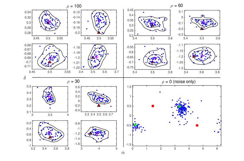
Figure 3: Maximum likelihood estimates (blue dots) of the GW source location in equatorial coordinates with 50 data realizations for the network SNR $\rho\neq 0$ and 200 for $\rho=0$ (noise only). The subpanels for each $\rho\neq 0$ panel correspond to the true locations A (top left), B (top right), C (bottom left) and D (bottom right), respectively. The true and estimated mean locations are marked by red triangles and magenta crosses respectively. The solid black lines show regions in which the probability of getting an estimated location is 68% and 95% (estimated using Kernel Density Estimation Botev et al. (2010)). In the $\rho=0$ panel, the center and anti-center of the Galaxy and its poles are marked by red squares and green stars respectively.

Limitations of the study and future work –

As is common in studies of isolated sources Ellis et al. (2012); Zhu et al. (2015), the signal from unresolved SMBHBs was ignored under the implicit assumption that it simply elevates the noise level. Future studies should test this assumption.

The fixed observed frequency of the signal in our simulation translates at a sufficiently high redshift into a rest frame frequency corresponding to a rapidly evolving phase of the binary Rosado et al. (2016). However, for the redshifted chirp masses considered here, this effect will only manifest itself at redshifts $z\gg 2$, the epoch of peak SMBHB formation rate, and may be ignored.

In the future, we plan to incorporate some form of regularization Rakhmanov (2006); Mohanty et al. (2006) in MaxPhase to mitigate the adverse effects of ill-posedness seen on source localization. The algorithm will be refined further by taking uncertainties in the measured noise parameters (Arzoumanian et al., 2016) into account. Additionally, it will be extended to include non-monochromatic signal models.