Entangled States of Two Quantum Dots Mediated by Majorana Fermions

Abstract

With the assistance of a pair of Majorana fermions, we propose schemes to entangle two quantum dots by Lyapunov control in the charge and spin degrees of freedom. Four different schemes are considered, i.e., the teleportation scheme, the crossed Andreev reflection scheme, the intra-dot spin flip scheme, and the scheme beyond intra-dot spin flip. We demonstrate that the entanglement can be generated by modulating the chemical potential of quantum dots with square pulses, which is easily realized in practice. In contrast to Lyapunov control, the preparation of entangled states by adiabatic passage is also discussed. There are two advantages in the scheme by Lyapunov control, i.e., it is flexible to choose a control Hamiltonian, and the control time is much short with respect to the scheme by adiabatic passage. Furthermore, we find that the results are quite different by different adiabatic passages in the scheme beyond intra-dot spin flip, which can be understood as an effect of quantum destructive interference.

I Introduction

Majorana fermions (MFs), which are predicted to exist at the boundary or in the vortex core of a topological superconductor (TS), have been widely studied recently both in theories kitaev01 ; qi11 ; alicea12 ; beenakker13 and experiments das2012 ; mourik12 ; rokhinoson12 ; lee13 ; perge14 . For example, MFs have been applied into topological quantum computation kitaev03 ; nayak08 due to their robustness against perturbations.

From the other aspect, two spatially separated MFs can form a Dirac fermion. This non-locality feature can offer the MFs an opportunity as the medium to entangle quantum systems such as quantum dots (QDs). The advantages to entangle QDs via MFs are twofold. Firstly, conventional schemes to entangle QDs are limited by spatial distance due to direct proximity coupling with each other loss98 ; petta05 ; koppens05 . As a result it is difficult to manipulate quantum states in such a small distance. The entanglement preparation mediated by MFs can effectively solve this drawback. Secondly, from the side of topological quantum computation, the MFs are difficult to couple together as the wave-function overlap of two MFs decays exponentially with spatial distance between them. Additionally, braiding operations solely are insufficient in the universal quantum computation for Majorana-based qubits nayak08 . Those difficulties can be availably overcomed in hybrid systems hassler11 ; sau10a ; jiang11 ; bonerson11 ; leijnse12a ; kovalev14 ; xue14 , where the combination of the robustness of topological qubits (e.g., Majorana-based qubit) and the universality of conventional qubits (e.g., QD-based qubit, flux qubit, etc.) can form an universal computation.

The adiabatic passage, which is widely applied to quantum information processing, is one way to prepare entanglement. The main idea is as follows. Given a quantum system that its ground state is separable and easy to prepare, one can adiabatically manipulate some physical parameters such that the system evolves into the ground state of the new Hamiltonian, which is the target entangled state. Since the adiabatic dynamics is protected, it is then immune to some types of perturbations. However, the price one should pay is the long time needed to finish the evolution. To overcome this difficulty, a shortcut to adiabaticity demirplak03 ; berry09 is introduced. The key point is that the time-dependent Hamiltonian $H_{1}(t)$ is brought into the Schrödinger equation. Nevertheless it is always hard to implement such a Hamiltonian for most systems, and $H_{1}(t)$ may not exist in complicated systems. This gives rise to a question—are there any other control strategies for the quantum system better than adiabatic passage?

In this work, we will focus on this issue. We propose to entangle two QDs by Lyapunov control, which has been employed in manipulating quantum states beauchard07 ; coron09 ; wang09 ; wang10a ; yi09 ; shi15 . The basic principle of Lyapunov control is to design control fields to drive a quantum system to approach the target state. Note that the target state must be a steady state such that the system cannot evolve when control fields vanish. In order to design control fields, a Lyapunov function has to be defined. To be specific, one first defines a Lyapunov function $V$ for the given target state $|\psi_{T}\rangle$. Then by restricting non-positivity of the time derivative of the Lyapunov function $V$ (i.e., $\dot{V}\leq 0$), one can obtain the control fields $f_{k}(t).$ Driven by these control fields, the system would evolve to the target state $|\psi_{T}\rangle$ with time.

The system we considered is a hybrid quantum system primarily consisting of two QDs and a TS wire with MFs. The two QDs are well spatially separated so that they do not have direct interaction, but they are coupled to a common TS wire. The entanglement between the two QDs is then induced via the non-locality property of the Dirac fermion defined by MFs. We adopt the Lyapunov control to explore entanglement generation in the following. For comparison, the entanglement generated by adiabatic passage is also presented and discussed.

II Model

The system under consideration is illustrated in Fig. 1(a), which consists of a TS wire coupled to two QDs and another bulk superconductor via tunneling. The free Hamiltonian of such a system contains two parts. The first part of the free Hamiltonian is for the TS wire ($\hbar=1$),

$$H_{0}^{TS}=\mathcal{H}_{TS}+\mathcal{H}_{TS}^{\prime},$$ (1)

where $\mathcal{H}_{TS}=\sum\xi_{k}\gamma_{k}^{{\dagger}}\gamma_{k}$. The energy spectrum is $\xi_{k}$, and the Bogoliubov quasiparticle operators $\gamma_{k}$ are related to the electron operators $c(x)$ of the TS wire in the standard way, where $x$ denotes the electron coordinate in the TS wire alicea12 . Note that we have dropped the spin subscript in this section as the spin degeneracy in the TS wire is broken due to Zeeman effect, which suggests that we might consider only one spin direction. Considering the situation that the TS wire is in the topological nontrivial phase, there is a pair of MFs $\gamma_{1}$ and $\bar{\gamma}_{1}$ at the ends of TS wire oreg10 ; lutchyn10 . This two zero-energy MFs can form a non-local Dirac fermion, i.e., $f=\frac{\gamma_{1}+i\bar{\gamma}_{1}}{2}$, where $f$ is the annihilation operator of Dirac fermion. When the energy scale of TS wire is smaller than the superconductor gap, there are no other quasiparticle excitations except for the zero-energy MFs in the TS wire. As a result we can safely ignore the Hamiltonian $\mathcal{H}_{TS}$ in the model. Note that when the TS wire is of mesoscopic size and is linked to a capacitor earth grounded, there exists an additional Hamiltonian $\mathcal{H}_{TS}^{\prime}$ describing the finite charging energy. The corresponding Hamiltonian takes fu10

$$\mathcal{H}_{TS}^{\prime}=E_{c}(2\hat{N}_{c}-n_{g}+n_{f})^{2},$$ (2)

where ${N}_{c}$ is the number of Cooper pairs, $n_{g}$ denotes the dimensionless gate charge determined by the gate voltage $V_{3}$, and $n_{f}=f^{{\dagger}}f$ stands for the number of Dirac fermion formed by MFs. The single electron charging energy is $E_{c}=\frac{e^{2}}{2C}$ with capacitance $C$. It has been shown that the single electron charging energy $E_{c}$ plays a key role in the long-range entanglement generation of two QDs plugge15 .

The second part of the free Hamiltonian is for the QDs,

$$H_{0}^{QD}=\sum_{n=1}^{2}\epsilon_{n}d_{n}^{{\dagger}}d_{n},$$ (3)

where $d_{n}$ and $d_{n}^{{\dagger}}$ are the annihilation and creation operations of electrons in the $n$-th QD. $\epsilon_{n}$ denotes the chemical potential which can be changed by the gate voltage $V_{n}$ ($n=1,2$). We should emphasize that we have assumed both QDs in the Coulomb block regime in Hamiltonian $H_{0}^{QD}$, i.e., the electron can only occupy single fermion level. This requires that $U_{n}$ [see in Eq. (22)] is large compared to the other relevant energy in the system.

Next we turn to the interaction Hamiltonian of system. The first term describes the Cooper pair exchange between the TS wire and the bulk superconductor,

$$H_{e}^{TS}=E_{J}\cos{\hat{\phi}}=\frac{E_{J}}{2}(e^{-i\hat{\phi}}+e^{i\hat{\phi}}).$$ (4)

$E_{J}$ is the Josephson coupling and $\phi$ is the phase difference between the two superconductors. Here the phase of bulk superconductor have been set to zero for simplicity. The operator $e^{-i\hat{\phi}}$ ($e^{i\hat{\phi}}$) represents the creation (annihilation) of a Cooper pair, i.e., $e^{-i\hat{\phi}}=\sum_{N_{c}}|N_{c}+1\rangle\langle N_{c}|$. The number operator of Cooper pairs and the phase of superconductor are canonically conjugate, i.e., $[\hat{N}_{c},e^{-i\hat{\phi}}]=e^{-i\hat{\phi}}$.

The second term of interaction Hamiltonian describes the electron tunneling between the TS wire and the QDs. For later use, we write down the electron operator $c(x)$ in terms of quasiparticle operator $\gamma_{k}$ in the TS wire, i.e., $c(x)=g_{1}\gamma_{1}+\bar{g}_{1}\bar{\gamma}_{1}+\cdots$, where $g_{k}$ is the wave function of spatial coordinate. As we have mentioned before, there are no other quasiparticles except for the MFs in the TS wire. This allows us to consider the first two terms in the expression of $c(x)$, i.e., $c(x)=g_{1}\gamma_{1}+\bar{g}_{1}\bar{\gamma}_{1}$. In addition, if the length of TS wire is large enough, there are no overlap between $g_{1}$ and $\bar{g}_{1}$, i.e., no coupling between $\gamma_{1}$ ($\bar{\gamma}_{1}$) and $d_{2}$ ($d_{1}$). As a consequence, the effective Hamiltonian describing tunnel coupling between electron in the QDs and Dirac fermion formed by the MFs is given by substituting $c(x)$ into the bare tunneling terms $\sim\int dxt_{n}d_{n}^{{\dagger}}c(x)+h.c.$ zazunov11 ; hutzen12 ; didier13 ,

$$H_{t}^{TQ}=\sum_{n=1}^{2}\lambda_{n}[f^{{\dagger}}+(-1)^{n-1}e^{-i\hat{\phi}}f]d_{n}+h.c.,$$ (5)

where $\lambda_{n}$ represents the coupling strength. In the derivation of Hamiltonian $H_{t}^{TQ}$, we have considered charge conservation since it cannot create or annihilate charge $2e$ without any energy cost in the TS wire with $E_{c}\neq 0$. In later discussion, the terms $f^{{\dagger}}d_{n}$ (or $d_{n}^{{\dagger}}f$) and $fd_{n}$ (or $d_{n}^{{\dagger}}f^{{\dagger}}$) are referred to the “normal” and “anomalous” tunneling process, respectively.

As we study the long-range entanglement generation in this paper, the length of TS wire is considered so sufficiently long that there does not exist direct coupling between the two MFs. Therefore the interaction Hamiltonian $H_{i}^{MF}=i\lambda_{f}\gamma_{1}\bar{\gamma}_{1}$ has also been neglected throughout this work.

Collecting these terms, we can write down the Hamiltonian for the whole system

$$H_{0}=H_{0}^{TS}+H_{0}^{QD}+H_{e}^{TS}+H_{t}^{TQ}.$$ (6)

In order to prepare maximally entangled state of the two QDs, e.g., Bell states, we choose $\epsilon_{1}=\epsilon_{2}=\epsilon$ and $\lambda_{1}=\lambda_{2}=\lambda$, and work in the large-$E_{c}$ limit (compared to the parameters $\epsilon$ and $\lambda$) which can always be satisfied by changing the size of TS wire. Since the total fermion parity, which is quantized by the number of the electrons in two QDs plus the Dirac fermion formed by MFs, is conserved in this model, we will study the even-parity case in the following. The extension from the even-parity case to the odd-parity case is straightforward.

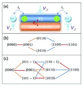
Figure 1: (a) Schematic illustration of the setup. A TS wire with strong spin orbit interaction is coupled to two QDs and a bulk superconductor via tunneling. The TS wire is deposited on a s-wave superconductor. When the TS wire is in the topological nontrivial phase due to the proximity effect and a Zeeman field, there exist a pair of MFs at the ends of TS wire. The chemical potentials of QDs can be changed by the gate voltage $V_{1,2}$, while the gate charge $n_{g}$ depends on the gate voltage $V_{3}$ of the capacitor (not shown in figure). (b) The transitions between distinct states with $n_{g}=1$. The red line represents the Josephson coupling while the orange and blue lines describe the “anomalous” and “normal” tunneling process, respectively. (c) The transition between distinct states with $n_{g}=0$.

III Teleportation scheme

The teleportation (TP) refers to nonlocal transfer of fermions across the TS wire plugge15 ; fu10 . As an example, we briefly present the physical process that electrons transfer from the first QD to the second QD via the TS wire. When an electron tunnels from the first QD to the TS wire, the charges in the TS wire increase one unit with energy cost $E_{c}$. If $E_{c}$ can not match $\epsilon$, the tunneling process is virtual. In order to keep the conservation of charge in the TS wire, the electron may transfer to the second QD. We first consider a case in which the Josephson coupling $E_{J}=0$ and the gate charge $n_{g}=1$. The ground state corresponds to that the number of Cooper pair $N_{c}=0$, Dirac fermion $n_{f}=1$, and the electrons $n_{1}+n_{2}=1$ in the even-parity case [cf., Eqs.(2)-(3)]. Namely, the ground states are $|0110\rangle$ and $|1010\rangle$. We have employed the notation $|n_{1}n_{2}n_{f}N_{c}\rangle$ to describe the system state, where $n_{1}$ ($n_{2}$) is the number of electrons in the first (second) QD, $n_{f}$ is the number of Dirac fermion formed by MFs, and $N_{c}$ is the number of Cooper pairs in the TS wire. $|0001\rangle$ and $|1100\rangle$ are the low excited states coupled directly to the ground state. We ignore the higher-energy excited states due to large gaps to the ground state. Since the entanglement generation is based on the nonlocality of the Dirac fermion defined by MFs [cf., Fig. 1(b)], we refer this proposal to teleportation scheme.

According to the transitions shown in Fig. 1(b), the Hilbert space is spanned by {$|0001\rangle$, $|0110\rangle$, $|1010\rangle$, $|1100\rangle$}. In this space, the Hamiltonian $H_{0}$ can be written as a $4\times 4$ matrix, i.e.,

$$H_{0}=\left(\begin{array}[]{cccc}E_{c}&-\lambda&\lambda&0\\ -\lambda&\epsilon&0&\lambda\\ \lambda&0&\epsilon&\lambda\\ 0&\lambda&\lambda&E_{c}+2\epsilon\\ \end{array}\right).$$ (11)

The system eigenstates then can be found analytically,

$$|E_{1}\rangle = \mathcal{N}_{1}(|1010\rangle-|0110\rangle-A_{1}|0001\rangle),$$

$$|E_{2}\rangle = \mathcal{N}_{2}(|1010\rangle-|0110\rangle+A_{2}|0001\rangle),$$

$$|E_{3}\rangle = \mathcal{N}_{3}(-\frac{A_{3}}{2}|1010\rangle-\frac{A_{3}}{2}|0110\rangle+|1100\rangle),$$

$$|E_{4}\rangle = \mathcal{N}_{4}(\frac{1}{A_{3}}|1010\rangle+\frac{1}{A_{3}}|0110\rangle+|1100\rangle),$$ (12)

and the corresponding eigenvalues are given by $E_{1}=\epsilon-\lambda A_{1}$, $E_{2}=E_{c}+\lambda A_{1}$, $E_{3}=E_{c}+2\epsilon-\lambda A_{3}$, $E_{4}=\epsilon+\lambda A_{3}$, where $A_{1}=\frac{\epsilon-E_{c}+\sqrt{(E_{c}-\epsilon)^{2}+8\lambda^{2}}}{2\lambda}$, $A_{2}=\frac{E_{c}-\epsilon+\sqrt{(E_{c}-\epsilon)^{2}+8\lambda^{2}}}{2\lambda}$, $A_{3}=\frac{E_{c}+\epsilon+\sqrt{(E_{c}+\epsilon)^{2}+8\lambda^{2}}}{2\lambda}$. $\mathcal{N}_{j}$ ($j=1,2,3,4$) is the normalization constant. One can find in Eq.(III) that $|E_{1}\rangle\simeq|0001\rangle$ if $\epsilon\gg E_{c}$, while if $\epsilon\ll E_{c}$, $|E_{1}\rangle\simeq\frac{1}{\sqrt{2}}(|10\rangle-|01\rangle)|10\rangle=|\psi_{T}\rangle,$ which is the Bell state of the two QDs. This observation paves the way towards preparing the Bell state $|\psi_{T}\rangle$ by adiabatic passage. To be explicit, we first initialize the system in state $|0001\rangle$. Then we adiabatically decrease the chemical potential $\epsilon$. The system would stay in the eigenstate $|E_{1}\rangle$, and arrive at the Bell state $|\psi_{T}\rangle$ finally. Similarly, when the initial state is $|1100\rangle$, the system would follow the eigenstate $|E_{3}\rangle$ to arrive at the Bell state.

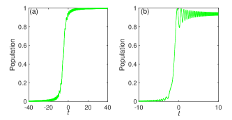
Figure 2: Population of the Bell state $|\psi_{T}\rangle$ as a function of time, where the population is defined as $|\langle\psi(t)|\psi_{T}\rangle|^{2}$. We have set the chemical potentials of the two QDs decrease with time linearly, e.g., $f(t)=-\frac{40}{T}t+20$. As a result the total manipulation time is $2T$. All parameters are in units of tunnel coupling $\lambda$. $E_{c}=30$, $\epsilon=5$. (a) $T=40$. (b) $T=10$.

In order to compare adiabatic passage with Lyapunov control, we reformulate the aforementioned results from the point of quantum control. That is, consider the chemical potentials of two QDs being manipulated in adiabatic passage, the control Hamiltonians read,

$$H_{1} = d_{1}^{{\dagger}}d_{1},$$

$$H_{2} = d_{2}^{{\dagger}}d_{2}.$$ (13)

Hence the system evolution is governed by the following Schrödinger equation,

$$i|\dot{\psi}\rangle=[H_{0}+\sum_{k=1}^{2}f_{k}(t)H_{k}]|\psi\rangle,$$ (14)

where $f_{k}(t)$ denotes the chemical potential changing with time. We refer $f_{k}(t)$ as control field hereafter, and set two control fields the same to simplify experimental realizations, i.e., $f_{1}(t)=f_{2}(t)=f(t)$. We plot in Fig. 2 the time evolution when linearly decreasing the chemical potentials of two QDs . It suggests that one can indeed achieve the Bell state $|\psi_{T}\rangle$ when the control fields $f(t)$ change sufficiently slowly with time [for instance, in Fig. 2(a)], but it takes long manipulation time. With increasing the change rate of chemical potentials, shown in Fig. 2(b), the performance gets worse due to the breakdown of adiabatic condition. Therefore the fact that it is difficult to decrease the manipulation time becomes a bottleneck for adiabatic passage.

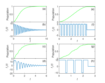
Figure 3: The system evolution as a function of time. Panel (a) is the population of Bell state $|\psi_{T}\rangle$ and the corresponding control field $f_{1}(t)$ is depicted in panel (b). The meaning of panels (c)-(d), panels (e)-(f), and panels (g)-(h) are the same as panels (a)-(b) except for different $B_{1}$ or $F$. All parameters are in units of the tunnel coupling $\lambda$. $E_{c}=20$, $\epsilon=5$. (b) $B_{1}=200$. (d) $B_{1}=300$. (f) $F=5$. (h) $F=10$.

Next we employ Lyapunov control to speedup the entanglement generation. In order to determine the form of control fields, one has to choose a Lyapunov function $V$ first, e.g.,

$$V=1-|\langle\psi_{T}|\psi\rangle|^{2},$$ (15)

where $|\psi_{T}\rangle$ is the target state (i.e., the Bell state). The first-order derivative of $V$ yields

$$\dot{V} = -2\sum_{k}f_{k}(t)\textrm{{Im}}[\langle\psi|\psi_{T}\rangle\langle\psi_{T}|H_{k}|\psi\rangle]$$

$$= -2\sum_{k}|\langle\psi|\psi_{T}\rangle|f_{k}(t)\textrm{{Im}}[e^{i\arg\langle\psi|\psi_{T}\rangle}\langle\psi_{T}|H_{k}|\psi\rangle],$$

where $\textrm{{Im}}(...)$ stands for the imaginary part of $(...)$ and $\textrm{arg}\langle\psi|\psi_{T}\rangle$ is the phase difference between $|\psi\rangle$ and $|\psi_{T}\rangle$. Thus, the condition $\dot{V}\leq 0$ can be satisfied naturally if we choose the control fields

$$f_{k}(t)=-B_{k}\textrm{{Im}}[e^{i\arg\langle\psi|\psi_{T}\rangle}\langle\psi_{T}|H_{k}|\psi\rangle],~{}~{}k=1,2,$$ (17)

where the constant $B_{k}>0$. Fig. 3(a)-(b) demonstrates how the system arrives at the Bell state $|\psi_{T}\rangle$ by control fields $f_{k}(t)$ when the initial state is $|0001\rangle$. In particular we have designed the control fields for both QDs to be the same, i.e., $f_{2}(t)=f_{1}(t)$. We further observe that the total manipulation time is related to the constant $B_{1}$, e.g., Fig. 3(c)-(d) are plotted with $B_{1}=300$. An inspection of Fig. 3(a)-(d) shows that the amplitude of control fields is time-dependent, which may make difficult for experimental realization. Actually, by the virtue of the fundamental principle of Lyapunov control, the dynamics performance is insensitive to the amplitude of control fields. Instead, it depends sharply on the sign of control fields. Due to this flexibility feature, the time-dependent amplitude of control fields can be replaced by square pulses as follows,

$$f_{k}(t)=\left\{\begin{array}[]{rl}F,~{}~{}~{}f_{k}(t)>0,\\ -F,~{}~{}~{}f_{k}(t)<0.\\ \end{array}\right.$$ (20)

Fig. 3 (e)-(h) show the performance to realize the Bell state $|\psi_{T}\rangle$ by square pluses, where the form of control fields are much simpler than that given by Eq. (17). Furthermore, the control time is also shortened by square pluses.

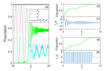
Figure 4: Population of the Bell state $|\psi_{T}\rangle$ (green-solid line) as a function of time in presence of the Josephson coupling $E_{J}=0.5$. Panel (a) demonstrates the results by adiabatic passage, while panels (b)-(e) demonstrate the system evolution by Lyapunov control. The red-dash (cyan-dash) line denotes the population of $|0000\rangle$ ($|0001\rangle$). $P\simeq 1$ (purple-solid) shows it has two major distinct physical mechanisms during the evolution, since the population of other states almost vanish. The other parameters are the same as in Fig. 3. (a) $T=20$. The control field in panel (c) is given by Eq.(17) with $B_{1}=300$, while it is calculated by Eq.(20) with $F=5$ in panel (e).

Now we turn to the case when existing the Josephson coupling. The Hilbert space is now spanned by $\{|0000\rangle,|0001\rangle,|0110\rangle,|1010\rangle,|1100\rangle,|1101\rangle\}$, as sketched in Fig. 1(b). We have neglected the higher-energy excited states once more. At first we decrease the chemical potentials of two QDs adiabatically when the initial state is $|0001\rangle$. The dynamical behaviors are plotted in Fig. 4(a). It can be observed that adiabatic passage is invalid for perfectly generating the Bell state $|\psi_{T}\rangle$ since the population cannot reach one. The reason can be found as follows. The evolution process mainly contains two physical mechanisms: (i) the Rabi oscillation between $|0000\rangle$ and $|0001\rangle$ for the existence of Josephson coupling; (ii) the population adiabatic transfer from $|0001\rangle$ to the Bell state $|\psi_{T}\rangle$. The population adiabatic transfer dominates only in the middle-stage and the throughout existence of Rabi oscillation lead to failure generation of the Bell state $|\psi_{T}\rangle$. But when employing Lyapunov control, we find in Fig. 4(b)-(e) that whether system exists the Josephson coupling makes no difference in the entanglement generation since the Bell state $|\psi_{T}\rangle$ is still the system eigenstate. The only difference from the aforementioned case is the shape of control field $f_{1}(t)$.

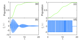
Figure 5: The population of the Bell state $|\psi_{T}\rangle$ as a function of time, where the control Hamiltonian is the Cooper pair exchange. (b) $B_{3}=100$. (d) $F=2$.

Alternatively, we can utilize the Cooper pair exchange between the TS wire and the bulk superconductor to be the control Hamiltonian in Lyapunov control, i.e.,

$$H_{3}=\cos\hat{\phi}=\frac{1}{2}(e^{-i\hat{\phi}}+e^{i\hat{\phi}}).$$ (21)

As shown in Fig. 5, the control field $f_{3}(t)$ designed by Eq.(17) or Eq.(20) can steer the system into the Bell state $|\psi_{T}\rangle$. Thus we can generate the Bell state $|\psi_{T}\rangle$ by modulating the strength of Cooper pairs exchange between the TS wire and the bulk superconductor.

IV Crossed Andreev reflection scheme

Crossed Andreev reflection (CAR), also known as nonlocal Andreev reflection, occurs when two spatially separated electrodes in normal state form two separate junctions with a superconductor. In our model a CAR process refers to the situation that two electrons from different QDs tunnel into the TS wire to form a Cooper pair plugge15 ; recher01 ; lesovik01 ; nilsson08 . Inversely, two electrons separated from a Cooper pair in the TS wire would tunnel into the QDs separately. Note that local Andreev reflection is absent since it cannot occupy two electrons for the same QD in the Coulomb block regime.

Recently, it has been shown that a strong and long-range coupling between two spatially separated QDs can be induced by a superconductor via CAR leijnse13 . Here in presence of MFs and charging energy $E_{c}$, we demonstrate that CAR can also be used to prepare long-range entanglement in two QDs when the parameters are $n_{g}=0$ and $\epsilon_{1}=-\epsilon_{2}=\epsilon$. The Hilbert space spanned by low-energy eigenstates is $\{|0000\rangle,|0001\rangle,|011-1\rangle,|0110\rangle,|1010\rangle,|101-1\rangle,|110-1\rangle,|1100\rangle\}$. Here we use the same notation $|n_{1}n_{2}n_{f}N_{c}\rangle$ as in the first case. With this basis, the Hamiltonian $H_{0}$ can be written as a $8\times 8$ matrix. As illustrated in Fig. 1(c), the entanglement can not be prepared without the Josephon coupling $E_{J}$. In other words, it requires Cooper pair exchange between the TS wire and the bulk superconductor. Hence we refer this process as crossed Andreev reflection scheme. Although the eigenstates can be calculated analytically, the expressions are tedious. Hence we adopt numerical solutions to discuss the occupation of the two lowest eigenstates of the Hamiltonian $H_{0}$.

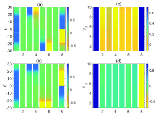
Figure 6: The probability amplitude of each basis appear in the two lowest eigenstates as a function of the chemical potential (panels (a)-(b)) and the Josephson coupling constant(panels (c)-(d)). The horizontal axis denotes the eight basis ordered as {$|0000\rangle$, $|0001\rangle$, $|011-1\rangle$, $|0110\rangle$, $|1010\rangle$, $|101-1\rangle$, $|110-1\rangle$, $|1100\rangle$}.

Fig. 6 shows that the eigenstate is nearly the Bell state $|\psi_{T}^{\pm}\rangle=(|00\rangle\pm|11\rangle)|00\rangle$ when $|\epsilon|<20$, and there is not an eigenstate that approximately equals one of the basis. This indicates that it is difficult to prepare the Bell state by adiabatic passage. To prepare the Bell state $|\psi_{T}^{+}\rangle$ by Lyapunov control, we first explore a situation that the control Hamiltonians are the particle number of the two QDs (i.e., $H_{n}=d_{n}^{{\dagger}}d_{n}$, $n=1,2$). With the control fields given by Eq.(17), we plot the results in Fig. 7(a). We find that the final state can be approximately expressed as $|\psi\rangle\approx\frac{1}{\sqrt{2}}(|00\rangle+|11\rangle)|00\rangle$, which is actually the Bell state. For the situation that the control Hamiltonian is the Cooper pair exchange (i.e., $H_{3}=\cos\hat{\phi}$), the results are plotted in Fig. 7(b). We find that the final state is not a Bell state, indicating it is fail to prepare the Bell state $|\psi_{T}^{+}\rangle$ in this situation. Further observations reveal that the populations on the basis {$|0000\rangle$, $|011-1\rangle$, $|0110\rangle$, $|1100\rangle$} nearly equal each other, which implies that the Bell state $|\psi_{T}^{+}\rangle$ may be obtained by measuring the parity of Dirac fermion. Indeed, further examination yields that if $n_{f}=0$, the final state collapses to $|\psi_{T}^{+}\rangle=\frac{1}{\sqrt{2}}(|00\rangle+|11\rangle)|00\rangle$. If $n_{f}=1$, the final state collapses to $|\psi\rangle\approx\frac{1}{\sqrt{2}}(|011-1\rangle+|0110\rangle)$, leading to the failure for generation of the Bell state $|\psi_{T}^{+}\rangle$.

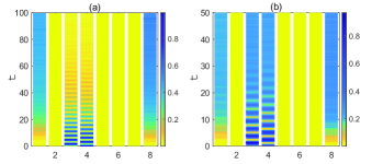
Figure 7: The population on each basis as a function of time. The eight basis are ordered as {$|0000\rangle$, $|0001\rangle$, $|011-1\rangle$, $|0110\rangle$, $|1010\rangle$, $|101-1\rangle$, $|110-1\rangle$, $|1100\rangle$} in horizontal axis. The initial state is $|0110\rangle$ and the target state is $|\psi_{T}^{+}\rangle=\frac{1}{\sqrt{2}}(|00\rangle+|11\rangle)|00\rangle$. The control Hamiltonians are (a) $H_{1}=d_{1}^{{\dagger}}d_{1}$, $H_{2}=d_{2}^{{\dagger}}d_{2}$, (b) $H_{3}=\cos\hat{\phi}$. All control fields are designed by Eq.(17).

V Scheme with intra-dot spin flip

In the last section, we propose a scheme to entangle two QDs regardless of electron spin states. We can also employ the spin up and spin down to encode quantum information due to their long coherence time loss98 ; petta05 ; koppens05 . In the following, we will investigate this issue.

As sketched in Fig. 8(a), the system differs not so much from the setup in Fig. 1(a). It does not have the bulk superconductor and the gate charge. In particular, in order to keeps spin degeneracy in QDs, we do not apply magnetic fields but employ a magnetic insulator contacting with the TS wire to induce the effective Zeeman coupling fu08 ; sau10 . The Hamiltonian reads flensberg11 ; leijnse11 ; tewari08 ; ke15

$$H_{0}^{\prime} = \sum_{n=1}^{2}\left(\sum_{\nu}\epsilon d_{n\nu}^{{\dagger}}d_{n\nu}+U_{n}d_{n\uparrow}^{{\dagger}}d_{n\uparrow}d_{n\downarrow}^{{\dagger}}d_{n\downarrow}+td_{n\uparrow}^{{\dagger}}d_{n\downarrow}\right)$$ (22)

$$+\lambda_{1}(f^{{\dagger}}+f)d_{1\downarrow}+\lambda_{2}(f^{{\dagger}}-f)d_{2\uparrow}+h.c.$$

The first term describes the energy of two QDs with the chemical potential $\epsilon$ for spin projection $\nu=\uparrow,\downarrow$. The second term describes two electrons occupying the same QD with Coulomb interaction $U_{n}$. In the Coulomb block regime, the electron can only occupy single fermion level in the two QDs, and we focus on this regime in the following. The third term describes the intra-dot spin flip with strength $t$, which stems from spin-orbit interactions and has been studied in Ref. khaetskii00 . Note that the spin of QD is no more a good quantum number as the transitions are allowed between distinct spin states. Since the spin flip term plays an essential role in the entanglement generation, as shown by the green line in Fig. 8(b), we will call this process the intra-dot spin flip scheme. The fourth (fifth) term describes the tunnel coupling between the Dirac fermion and the spin down (up) electron in the first (second) QD with strength $\lambda_{1}$ ($\lambda_{2}$).

In general, the MFs always have a definite spin polarization at the two ends of TS wire. Thus the wire can only send or receive electrons with the same spin polarization. The spin polarization of MFs are determined by the boundary between topological and non-topological regions sticlet12 ; kjaergaard12 , which are antiparallel at the two ends of TS wire oreg10 ; fu08 in an ideal case. We should emphasize that the spin polarization is not antiparallel in real cases, which would cause an error in the entanglement preparation leijnse12a . Nevertheless, we can manipulate the chemical potentials around the ends of TS wire to achieve nearly perfect antiparallel spin polarization. This is the reason why in the fourth (fifth) term we have assumed the electron state is spin down (up) on the left (right) MF $\gamma_{1}$ ($\bar{\gamma}_{1}$), and it can be only coupled to the spin down (up) electron in the first (second) QD via tunneling.

When we consider the even-parity case, the Hilbert space is spanned by {$|000\rangle$, $|\downarrow 01\rangle$, $|0\uparrow 1\rangle$, $|\uparrow 01\rangle$, $|0\downarrow 1\rangle$, $|\downarrow\uparrow 0\rangle$, $|\uparrow\uparrow 0\rangle$, $|\uparrow\downarrow 0\rangle$, $|\downarrow\downarrow 0\rangle$}. We have employed the label $|n_{1}n_{2}n_{f}\rangle$ to describe system state, where $n_{1}(n_{2})=0,\uparrow,\downarrow$ denotes the electron state in the first (second) QD and $n_{f}$ denotes the number of Dirac fermion combined by MFs. Note that the Hamiltonian $H_{0}^{\prime}$ can be represented by a $9\times 9$ matrix in these basis. As the analytical expressions of system eigenstates are involved, we choose to show the behaviors of two lowest eigenstates by numerical calculations.

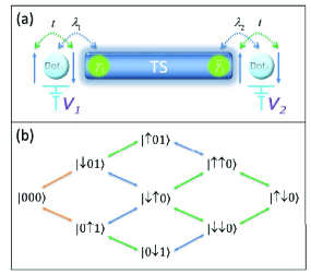
Figure 8: The schematic setup consisting of a TS wire tunnel coupling to two QDs. Only spin down (up) electron in the first (second) QD can be tunnel coupled to the TS wire since the left (right) MF $\gamma_{1}$ ($\bar{\gamma}_{1}$) is spin down (up) as well. At the same time, there exists the intra-dot spin flip process in two QDs. (b) The transition between distinct states. The green line represents the intra-dot spin flip process.

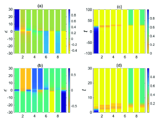
Figure 9: The amplitude of each basis in two lowest eigenstates as a function of the chemical potential in panels (a)-(b). The horizontal axis denotes the nine basis ordered as {$|000\rangle$, $|\downarrow 01\rangle$, $|0\uparrow 1\rangle$, $|\uparrow 01\rangle$, $|0\downarrow 1\rangle$, $|\downarrow\uparrow 0\rangle$, $|\uparrow\uparrow 0\rangle$, $|\uparrow\downarrow 0\rangle$, $|\downarrow\downarrow 0\rangle$}. One can find that the amplitude mainly locates at basis $|000\rangle$ when $\epsilon\gg 0$ in panel (a), while the amplitude mainly equal-weighted locates at basis $|\uparrow\uparrow 0\rangle$ and $|\downarrow\downarrow 0\rangle$ when $\epsilon\ll 0$ in panel (b). The population of each basis as a function of time in panels (c)-(d). $\epsilon=-10$. The control fields are (c) $f(t)=-\frac{2}{5}t+20$ in adiabatic passage, (d) designed by Eq.(17) with $B_{1}=1000$ in Lyapunov control. After completing controls, the amplitude of final state mainly equal-weighted locates at basis $|\uparrow\uparrow 0\rangle$ and $|\downarrow\downarrow 0\rangle$.

Fig. 9(a)-(b) describes the amplitude of each basis in two lowest eigenstates as a function of the chemical potential. It demonstrates that the eigenstate approximately equals to the state $|000\rangle$ when the chemical potential $\epsilon\gg 0$, while the eigenstate nearly becomes the Bell state $|\psi_{T}^{\prime}\rangle=(|\uparrow\uparrow\rangle-|\downarrow\downarrow\rangle)|0\rangle$ when the chemical potential $\epsilon\ll 0$. In addition to this we find in Fig. 8(b) that the transition path $|000\rangle\leftrightarrow|\uparrow\uparrow 0\rangle$ and the transition path $|000\rangle\leftrightarrow|\downarrow\downarrow 0\rangle$ are completely symmetric so that it is possible to generate the Bell state by adiabatic passage. The main control procedures are as follows. The system is initialized in the state $|000\rangle$ with large chemical potential. Then we adiabatically decrease the chemical potential. The system would evolve to the Bell state $|\psi_{T}^{\prime}\rangle=(|\uparrow\uparrow\rangle-|\downarrow\downarrow\rangle)|0\rangle$ finally, which is plotted in Fig. 9(c). An universal drawback of adiabatic passage is that it takes long control time in order to meet adiabatic condition. To reduce the control time we turn to Lyapunov control, where the control fields are designed by Eq.(17) instead of decreasing gradually (in adiabatic control). The dynamics evolution is demonstrated in Fig. 9(d). One can find the total control time of implementing the Bell state $|\psi_{T}^{\prime}\rangle$ by Lyapunov control is much shorter than that by adiabatic passage.

VI Scheme beyond intra-dot spin flip

We can also prepare the Bell states based on a scheme beyond intra-dot spin flip. The system considered is composed of two TS wires coupling to two common QDs, as illustrated in Fig. 10(a). The Hamiltonian describing such a system reads flensberg11 ; leijnse11 ; tewari08

$$H_{0}^{\prime\prime} = \sum_{n=1}^{2}\Big{(}\sum_{\nu}\epsilon d_{n\nu}^{{\dagger}}d_{n\nu}+U_{n}d_{n\uparrow}^{{\dagger}}d_{n\uparrow}d_{n\downarrow}^{{\dagger}}d_{n\downarrow}+\lambda_{n+1}[f_{n}^{{\dagger}}-$$

$$(-1)^{n-1}f_{n}]d_{n+1\uparrow}+\lambda_{n}[f_{n}^{{\dagger}}+(-1)^{n-1}f_{n}]d_{n\downarrow}+h.c.\Big{)},$$

where the notation is the same as in Eq.(22), and we adopt the convention $n\mod 2$ if $n>2$. We use $|n_{1}n_{2}n_{f_{1}}n_{f_{2}}\rangle$ to denote system state, where $n_{1}(n_{2})=0,\uparrow,\downarrow$ stands for an electron state in the first (second) QD and $n_{f_{1}}=f_{1}^{{\dagger}}f_{1}$ ($n_{f_{2}}=f_{2}^{{\dagger}}f_{2}$) denotes the number of Dirac fermion defined by MFs in the left (right) TS wire.

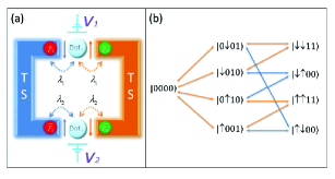
Figure 10: (a) The schematic setup consisting of two TS wires tunnel coupling to two QDs. (b) The transition between distinct states.

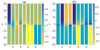
Figure 11: The amplitude of each basis in two lowest eigenstates as a function of the chemical potential. The horizontal axis denotes the nine basis ordered as {$|0000\rangle$, $|0\downarrow 01\rangle$, $|\downarrow 010\rangle$, $|0\uparrow 10\rangle$, $|\uparrow 001\rangle$, $|\downarrow\downarrow 11\rangle$, $|\uparrow\downarrow 00\rangle$, $|\downarrow\uparrow 00\rangle$, $|\uparrow\uparrow 11\rangle$}.

Similar to the analysis presented in the last section, we first analyze the behaviors of the two lowest eigenstates as a function of chemical potential with numerical simulations. When $\epsilon\gg 0$, the eigenstate is very close to the basis $|0000\rangle$ [see Fig. 11(a)]. When $\epsilon\ll 0$, the eigenstate is approximately a superposition of $|\downarrow\downarrow 11\rangle$ and $|\uparrow\uparrow 11\rangle$ with almost equal weight [see Fig. 11(b)]. It is believed that the system can be steered into the Bell state by adiabatic passage when the initial state is $|0000\rangle$. Here we explore this issue by two different adiabatic passages. The first is to simultaneously decrease the chemical potentials of the two QDs with the same rate, as shown in Fig. 12(a). The system finally is driven into the Bell state $|\psi_{1}\rangle=\frac{1}{\sqrt{2}}(|\downarrow\downarrow\rangle+|\uparrow\uparrow\rangle)|11\rangle$. Another method is to adiabatically decrease the chemical potential of the first QD while the chemical potential of the second QD remains unchanged. After completing this operation, the system state becomes $|\psi^{\prime}\rangle=\frac{1}{\sqrt{2}}(|\downarrow 010\rangle+|\uparrow 001\rangle)$. We then adiabatically decrease the chemical potential of the second QD while the chemical potential of the first QD remains unchanged. The results are shown in Fig. 12(b). The final state of system becomes $|\psi\rangle=\frac{1}{2}(|\uparrow\downarrow\rangle+|\downarrow\uparrow\rangle)|00\rangle-\frac{1}{2}(|\downarrow\downarrow\rangle+|\uparrow\uparrow\rangle)|11\rangle$, which is actually not the Bell state of the two QDs. However, with the help of measurement results on the Dirac fermion parity (e.g., $n_{f_{1}}$), the system would collapse into Bell state $|\psi_{2}\rangle=\frac{1}{\sqrt{2}}(|\uparrow\downarrow\rangle+|\downarrow\uparrow\rangle)|00\rangle$ if $n_{f_{1}}=0$, while the system would collapse to Bell state $|\psi_{1}\rangle=\frac{1}{\sqrt{2}}(|\downarrow\downarrow\rangle+|\uparrow\uparrow\rangle)|11\rangle$ if $n_{f_{1}}=1$. Remarkably, the control results are quite different for the two adiabatic passages. This originates from the fact that it exists quantum destructive interference in the first adiabatic passage. To clarify this point, we examine the transition paths between $|0000\rangle$ and $|\uparrow\downarrow 00\rangle$ in Fig. 10(b), i.e.,

$$|0000\rangle \xlongleftrightarrow{-\lambda_{2}} |0\downarrow 01\rangle\xlongleftrightarrow{\lambda_{1}}|\uparrow\downarrow 01\rangle,$$

$$|0000\rangle \xlongleftrightarrow{\lambda_{1}} |\uparrow 001\rangle\xlongleftrightarrow{\lambda_{2}}|\uparrow\downarrow 01\rangle.$$

Due to the presence of minus sign in the coupling constant, these two transition paths destructively interfere in the first method (The mechanism is same for the transition paths between $|0000\rangle$ and $|\downarrow\uparrow 00\rangle$). But this effect cannot happen in the second method.

From the aspect of Lyapunov control, since both $|\psi_{1}\rangle$ and $|\psi_{2}\rangle$ are the eigenstates of the system when $\epsilon\ll 0$ ($|\psi_{2}\rangle$ is not shown in Fig. 11), it is then possible to generate Bell states by Lyapunov control, where the control fields are designed by Eq.(17). The results are presented in Fig. 12(c)-(d). Compared with the adiabatic control, a specific type of Bell states (e.g., $|\psi_{1}\rangle$ and $|\psi_{2}\rangle$) can be prepared without measurement.

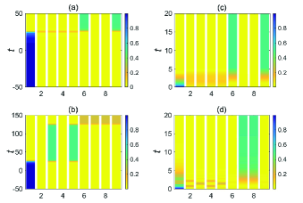
Figure 12: The population on each basis as a function of time when the initial state is $|0000\rangle$. The horizontal axis denotes the nine bases ordered as {$|0000\rangle$, $|0\downarrow 01\rangle$, $|\downarrow 010\rangle$, $|0\uparrow 10\rangle$, $|\uparrow 001\rangle$, $|\downarrow\downarrow 11\rangle$, $|\uparrow\downarrow 00\rangle$, $|\downarrow\uparrow 00\rangle$, $|\uparrow\uparrow 11\rangle$}. It presents two distinct adiabatic methods: (a) simultaneously decreasing the chemical potential of two QDs with the same rate, i.e., $f_{1}(t)=f_{2}(t)=-\frac{6}{5}t+30$. (b) decreasing the chemical potential of two QDs in turns, i.e., $f_{1}(t)=-\frac{6}{5}t+30,t\in[-50,50]$, and $f_{2}(t)=-\frac{6}{5}(t-100)+30,t\in[50,150]$. $f_{1}(t)=f_{2}(t)=0$ for other evolution time. Deterministic generation of two Bell states $|\psi_{1}\rangle$ and $|\psi_{2}\rangle$ in Lyapunov control while the target state is (c) $|\psi_{1}\rangle=(|\downarrow\downarrow\rangle+|\uparrow\uparrow\rangle)|11\rangle$, (d) $|\psi_{2}\rangle=(|\uparrow\downarrow\rangle+|\downarrow\uparrow\rangle)|00\rangle$.

VII Discussion and conclusion

Before concluding, we discuss the validity of the assumptions made in our model and the experimental feasibility of our proposal.

The first assumption in this work is that there are no other quasiparticles in the TS wire except for MFs. This assumption is true if the gap $\Delta$ in the superconductor is sufficiently large. Recent experiments das2012 ; mourik12 ; deng12 ; finck13 ; higginbotham15 report the observation of MFs in the TS wire (e.g., InAs or InSb nanowire) and the superconducting gap $\Delta$ is in the order of 0.1-1 meV, which is much larger than thermal fluctuations $\sim k_{B}T$ with temperature $\lesssim$100 mK.

In the second assumption, we suppose that both QDs are in the Coulomb block regime. Experimentally, the two QDs can be constructed at the two ends of the same TS wire. The electrostatic gates underneath the TS wire create a confinement potential for electron to form a QD. It have been demonstrated that the Coulomb interaction $U$ in such QD device is in the order of 1-10 meV fasth07 ; nilsson09 , which is much larger than the superconducting gap $\Delta$ and the thermal fluctuation at operating temperature. Therefore the QDs in the Coulomb block regime is realistic in our model.

Besides, the charging energy $E_{c}$ is also an essential parameter for generating long-range entanglement, which is in the order of $1$ meV higginbotham15 . To meet the condition $E_{c}<\Delta$, one can increase the length of TS wire or capacitance to reduce the charging energy $E_{c}$. If the charging energy $E_{c}$ is larger than the superconducting gap $\Delta$, quasiparticles would appear in the TS wire, which participate in the entanglement preparation. When such quasiparticles are in the bulk of TS wire, i.e., no remarkable overlap with MFs, they do not have effect on the Bell state preparation. Nevertheless, when the quasiparticles are located near the ends of TS wire, it may be invalid to prepare the Bell states by adiabatic passage or Lyapunov control.

Since the chemical potential of QDs can be modulated by electrostatic gates, we mainly discuss how to change the gate voltage to simulate the control fields. To prepare the Bell states by adiabatic passage, we just need to decrease the gate voltage with time linearly, which is easily realized in experiments. In Lyapunov control, it may not be easy to manipulate the gate voltage to simulate the time-dependent amplitude of control fields [e.g., Fig. 3(b)], but it is quite easy to realize the square pulses required by the control fields [e.g., Fig. 3(f)]. One may notice that the tunnel coupling $\lambda$ is fixed in our calculation. In fact, the tunnel coupling depends on both the chemical potential of QDs and tunneling barriers. As the tunnel coupling changes with the chemical potentials of QDs, but one can employ additional electrostatic gates on tunnel barriers to keep the tunnel coupling fixed perge10 .

Finally, we discuss the effect of decoherence on the preparation of Bell states in charge qubit, since the spin qubit has a coherence time (in the order of microseconds) longer than charge qubit. Due to the electron-phonon interactions, an intrinsic decoherence mechanism in QDs, the lifetime of charge qubit is in the order of $16$ ns petta04 ; petersson10 . In realistic situations, the tunnel coupling $\lambda$ can be modulated by electrostatic gates and reach the order of 1-10 $\mu$eV, so the total manipulation time is in the order of 6-60 ns by adiabatic passage. Hence the adiabatic passage would be invalid for Bell states preparation if the tunnel coupling $\lambda$ is too weak. However the manipulation time is in the order of 0.7-7 ns by Lyapunov control, which is much shorter than the lifetime of charge qubit. Therefore Lyapunov control is feasible for entangled state preparation when the tunnel coupling is not very large.

In conclusion, by the teleportation scheme, the crossed Andreev reflection scheme, the intra-dot spin flip scheme, and the scheme beyond intra-dot spin flip, we show how to entangle two QDs mediated by a pair of MFs. The Bell states can be prepared in both the charge degrees and spin degrees of QDs by Lyapunov control. In contrast, we compare our results with those by adiabatic passage. The Lyapunov control manifests advantages over adiabatic passage at flexibility designing control fields and accelerating control time.

In the teleportation scheme, the system can be driven into Bell state $|\psi_{T}\rangle=\frac{1}{\sqrt{2}}({|10\rangle-|01\rangle})|10\rangle$ by both adiabatic passage and Lyapunov control when the initial state is $|0001\rangle$. When the Josephson coupling is taken into account, it is not available to prepare Bell states perfectly by adiabatic passage due to the existence of Rabi oscillation. However, the Lyapunov control can still work well by modulating the shape of control fields. In addition, we find that the Cooper pair exchange can also be served as the control Hamiltonian to generate Bell states. In the crossed Andreev reflection scheme, since it does not exist a low-energy eigenstate whose amplitude mainly locates at one of the basis, we directly turn to Lyapunov control. The results show that the system can reach the Bell state $|\psi_{T}^{+}\rangle=\frac{1}{\sqrt{2}}(|00\rangle+|11\rangle)|00\rangle$ when we regulate the chemical potentials of two QDs. However, if we choose the Cooper pair exchange as control Hamiltonian, whether it can generate the Bell state successfully or not depends on parity measurement results of the Dirac fermion formed by MFs.

As to the entanglement in the spin degree of freedom, we have studied the system in the presence of intra-dot spin flip process. Through exploring the low-energy eigenstates of the system, it demonstrates that one can achieve the Bell state $|\psi_{T}^{\prime}\rangle=(|\uparrow\uparrow\rangle-|\downarrow\downarrow\rangle)|0\rangle$ by both adiabatic passage and Lyapunov control. For the scheme beyond intra-dot spin flip, the system consists of two TS wires and two QDs. Interestingly, we find that the results are quite different in distinct adiabatic passages, i.e., decreasing the chemical potentials of two QDs simultaneously or in turns. This diversity originates from whether existing quantum destructive interference in adiabatic evolution. Finally we have showed that the system can be certainly driven into distinct Bell states by Lyapunov control.

References

- (1) A. Kitaev, Phys. Usp. 44, 131 (2001).
- (2) X. L. Qi and S. C. Zhang, Rev. Mod. Phys. 83, 1057 (2011).
- (3) J. Alicea, Rep. Prog. Phys. 75, 076501 (2012).
- (4) C. W. J. Beenakker, Annu. Rev. Condens. Mat. Phys. 4, 113 (2013).
- (5) A. Das, Y. Ronen, Y. Most, Y. Oreg, M. Heiblum, and H. Shtrikman, Nat. Phys. 8, 887 (2012).
- (6) V. Mourik, K. Zuo, S. M. Frolov, S. R. Plissard, E. P. A. M. Bakkers, and L. P. Kouwenhoven, Science, 336, 1003 (2012).
- (7) L. P. Rokhinson, X. Liu, and J. K. Furdyna, Nat. Phys. 8, 795 (2012).
- (8) E. J. H. Lee, X.Jiang, M. Houzet, R. Aguado, C. M. Lieber, and S. D. Franceschi, Nat. Nanotech. 9, 79-84 (2014).
- (9) S. N. Perge, I. K. Drozdov, J. Li, H. Chen, S. Jeon, J. Seo, A. H. MacDonald, B. A. Bernevig, and A. Yazdani, Science, 346, 602 (2014).
- (10) A. Y. Kitaev, Ann. Phys. 303, 2 (2003).
- (11) C. Nayak, S. H. Simon, A. Stern, M. Freedman, and S. Das Sarma, Rev. Mod. Phys. 80, 1083 (2008).
- (12) D. Loss, D. P. Di Vincenzo, Phys. Rev. A 57, 120 (1998).
- (13) J. R. Petta, A. C. Johnson, J. M. Taylor, E. A. Laird, A. Yacoby, M. D. Lukin, C. M. Marcus, M. P. Hanson, A. C. Gossard, Science 309, 2180 (2005).
- (14) F. H. L. Koppens, J. A. Folk, J. M. Elzerman, R. Hanson, L. H. W. van Beveren, I. T. Vink, H. P. Tranitz, W. Wegscheider, L. P. Kouwenhoven, L. M. K. Vandersypen, Science 309, 1346 (2005).
- (15) F. Hassler, A. R. Akhmerov, C. Y. Hou, and C. W. J. Beenakker, New J. Phys. 12, 125002 (2010).
- (16) J. D. Sau, S. Tewari, and S. D. Sarma, Phys. Rev. A 82, 052322 (2010).
- (17) L. Jiang, C. L. Kane, and J. Preskill, Phys. Rev. Lett. 106, 130504 (2011).
- (18) P. Bonderson and R. M. Lutchyn, Phys. Rev. Lett. 106, 130505 (2011).
- (19) M. Leijnse and K. Flensberg, Phys. Rev. B 86, 104511 (2012).
- (20) A. A. Kovalev, A. De, and K. Shtengel, Phys. Rev. Lett. 112, 106402 (2014).
- (21) Z. Y. Xue, M. Gong, J. Liu, Y. Hu, S. L. Zhu, and Z. D. Wang, Sci. Rep. 5, 12233 (2015).
- (22) M. Demirplak and S. A. Rice, J. Phys. Chem. A 107, 9937 (2003).
- (23) M. V. Berry, J. Phys. A: Math. Theor. 42, 365303 (2009).
- (24) K. Beauchard, J. M. Coron, M. Mirrahimi, and Z. Rouchon, Systems and Control Letters. 56, 388 (2007).
- (25) J. M. Coron, A. Grigoriu, C. Lefter, and G. Turinici, New J. Phys. 11, 105034 (2009).
- (26) X. T. Wang and S. G. Schirmer, Phys. Rev. A 80, 042305 (2009).
- (27) X. X. Yi, X. L. Huang, C. F. Wu and C. H. Oh, Phys. Rev. A 80, 052316 (2009).
- (28) X. T. Wang, A. Bayat, S. Bose, and S. G. Schirmer, Phys. Rev. A 82, 012330 (2010).
- (29) Z. C. Shi, X. L. Zhao, and X. X. Yi, Phys. Rev. A 91, 032301 (2015).
- (30) Y. Oreg, G. Refael, and F. von Oppen, Phys. Rev. Lett. 105, 177002 (2010).
- (31) R. M. Lutchyn, J. D. Sau, and S. Das Sarma, Phys. Rev. Lett. 105, 077001 (2010).
- (32) L. Fu, Phys. Rev. Lett. 104, 056402 (2010).
- (33) S. Plugge, A. Zazunov, P. Sodano, and R. Egger, Phys. Rev. B 91, 214507 (2015).
- (34) A. Zazunov, A. L. Yeyati, and R. Egger, Phys. Rev. B 84, 165440 (2011).
- (35) R. Hützen, A. Zazunov, B. Braunecker, A. L. Yeyati, and R. Egger, Phys. Rev. Lett. 109, 166403 (2012).
- (36) N. Didier, M. Gibertini, A. G. Moghaddam, J. König, and R. Fazio, Phys. Rev. B 88, 024512 (2013).
- (37) P. Recher, E. V. Sukhorukov, and D. Loss, Phys. Rev. B 63, 165314 (2001).
- (38) G. B. Lesovik, T. Martin, and G. Blatter, Eur. Phys. J. B 24, 287 (2001).
- (39) J. Nilsson, A. R. Akhmerov, and C. W. J. Beenakker, Phys. Rev. Lett. 101, 120403 (2008).
- (40) M. Leijnse and K. Flensberg, Phys. Rev. Lett. 111, 060501 (2013).
- (41) L. Fu and C. L. Kane, Phys. Rev. Lett. 100, 096407 (2008).
- (42) J. D. Sau, R. M. Lutchyn, S. Tewari, and S. D. Sarma, Phys. Rev. Lett. 104, 040502 (2010).
- (43) S. Tewari, C. Zhang, S. Das Sarma, C. Nayak, and D. H. Lee, Phys. Rev. Lett. 100, 027001 (2008).
- (44) K. Flensberg, Phys. Rev. Lett. 106, 090503 (2011).
- (45) M. Leijnse and K. Flensberg, Phys. Rev. Lett. 107, 210502 (2011).
- (46) S. S. Ke, H. F. Lv, H. J. Yang, Y. Guo, H. W. Zhang, Phys. Lett. A 379, 170 (2015).
- (47) A. V. Khaetskii and Y. V. Nazarov, Phys. Rev. B 61, 12639 (2000).
- (48) D. Sticlet, C. Bena, and P. Simon, Phys. Rev. Lett. 108, 096802 (2012).
- (49) M. Kjaergaard, K. Wölms, and K. Flensberg, Phys. Rev. B 85, 020503 (2012).
- (50) M. T. Deng, C. L. Yu, G. Y. Huang, M. Larsson, P. Caroff, H. Q. Xu, Nano Lett. 12, 6414 (2012).
- (51) A. D. K. Finck, D. J. Van Harlingen, P. K. Mohseni, K. Jung, X. Li, Phys. Rev. Lett. 110, 126406 (2013).
- (52) A. P. Higginbotham, S. M. Albrecht, G. Kirsanskas, W. Chang, F. Kuemmeth, P. Krogstrup, T. S. Jespersen, J. Nygard, K. Flensberg, and C. M. Marcus, arXiv:1501.05155 (2015).
- (53) C. Fasth, A. Fuhrer, L. Samuelson, V. N. Golovach, and D. Loss, Phys. Rev. Lett. 98, 266801 (2007).
- (54) H. A. Nilsson, P. Caroff, C. Thelander, M. Larsson, J. B. Wagner, L. E. Wernersson, L. Samuelson, and H. Q. Xu, Nano Lett. 9, 3151 (2009).
- (55) S. Nadj-Perge, S. M. Frolov, E. P. A. M. Bakkers, and L. P. Kouwenhoven, Nature, 468, 1084 (2010).
- (56) J. R. Petta, A. C. Johnson, C. M. Marcus, M. P. Hanson, and A. C. Gossard, Phys. Rev. Lett. 93, 186802 (2004).
- (57) K. D. Petersson, J. R. Petta, H. Lu, and A. C. Gossard, Phys. Rev. Lett. 105, 246804 (2010).