Laughlin’s argument for the quantized thermal Hall effect

Abstract

We extend Laughlin’s magnetic-flux-threading argument to the quantized thermal Hall effect. A proper analogue of Laughlin’s adiabatic magnetic-flux threading process for the case of the thermal Hall effect is given in terms of an external gravitational field. From the perspective of the edge theories of quantum Hall systems, the quantized thermal Hall effect is closely tied to the breakdown of large diffeomorphism invariance, that is, a global gravitational anomaly. In addition, we also give an argument from the bulk perspective in which a free energy, decomposed into its Fourier modes, is adiabatically transferred under an adiabatic process involving external gravitational perturbations.

I Introduction

The thermal Hall conductivity is quantized in gapped $(2+1)$-dimensional topological phases Prange and Girvin (1987); Hasan and Kane (2010); Qi and Zhang (2011) of charged and charge-neutral excitation systems. Integer and fractional quantum Hall systems Kane and Fisher (1997) and chiral p-wave topological superconductors Read and Green (2000) are examples of such systems. More precisely, the thermal Hall conductivity in these systems is given by

$$\kappa_{H}=c\frac{\pi k_{\text{B}}^{2}T}{6\hbar},$$ (1)

where $c$ is the chiral central charge of the gapless boundary modes. Hence, $\kappa_{H}$ is quantized in units of $\pi k_{\text{B}}^{2}T/6\hbar$. For example, an integer quantum Hall system with the bulk Chern number $\nu$ of the filled electronic energy bands has $\nu$ complex-fermionic boundary modes with $c=\nu$, and a topological superconductor with the Chern number $\nu$ of the Bogoliubov quasiparticles has $\nu$ Majorana boundary modes with $c=\nu/2$.

The quantized thermal Hall effect in two-dimensional topological insulators and topological superconductors (superfluids) has been discussed both from bulk and boundary points of view. From the perspective of chiral gapless boundary theories, the thermal Hall effect has been studied in terms of the chiral Luttinger liquid Kane and Fisher (1997), the conformal field theory Cappelli et al. (2002); Bradlyn and Read (2015a), the gravitational Chern-Simons theory Stone (2012), and the equilibrium partition function Nakai et al. (2016). On the other hand, the thermal Hall effect in the quantum Hall bulk is much controversial. Various studies using the Kubo formula Smrcka and Streda (1977); Cooper et al. (1997); Qin et al. (2011), the non-equilibrium Green’s function Shitade (2014), and the Středa formula Nomura et al. (2012) have concluded that the bulk fermionic states show the quantized thermal Hall effect. However, from the point of view of equilibrium thermal field theories, the thermal Hall current in the bulk is exponentially small when the temperature is much smaller than the bulk energy gap Mañes and Valle (2013). Also, an induced gravitational field theory derived from a fully gapped fermionic system in a thermal equilibrium cannot describe the quantized thermal Hall effect Bradlyn and Read (2015b). These results may imply that, while for chiral edge theories one can develop an argument for the quantized thermal Hall effect, parallel to the quantum Hall effect, the bulk picture of the quantized thermal Hall effect may be distinct from that for the quantum Hall effect.

In this paper, we extend the gauge invariance/noninvariance argument presented by Laughlin Laughlin (1981) to the thermal Hall effect in quantum Hall systems. Laughlin’s argument provides a fundamental and robust theory of adiabatic responses in gapped topological phases. We will make an attempt to follow as closely as possible the original Laughlin’s argument, by making one-to-one correspondence between electromagnetism and gravity (or more precisely, not full Einstein gravity but gravitoelectromagnetism). We will discuss the adiabatic responses of the chiral boundary fermion modes and the bulk quantum Hall states against the gravitational counterpart of the magnetic-flux threading.

From the edge-theoretical point of view, we elucidate the role of quantum anomalies connecting the boundary theories and Laughlin’s argument. In particular, we will make use of the global gravitational anomaly of the boundary theories, as opposed to the perturbative gravitational anomaly. While the perturbative gravitational anomaly correctly accounts for the non-conservation of the energy-momentum of the chiral edge theories, and hence the necessity of having the bulk system, it is not entirely obvious how one could relate the non-conservation of the energy-momentum to the thermal transport. As we will discuss, the connection to the thermal transport is more transparent if we base our discussion on the global gravitational anomaly. It should however be noted that the global gravitational anomaly, i.e., the anomalous phase of the partition function, has an ambiguity $2\pi\times\mbox{integer}$. One may then worry that the global gravitational anomaly may not have an ability to fix the thermal transport coefficient entirely. Nevertheless, this ambiguity can be lifted by requiring consistency with the perturbative gravitational anomaly.

As for the bulk point of view, our thermal extension of Laughlin’s argument reveals a picture quite analogous to the quantized charge Hall current that flows adiabatically through the bulk, i.e., the creeping of Landau orbitals as one threads a magnetic flux adiabatically. In particular, to explain the thermal Hall effect, it seems that it is possible to avoid the use of non-equilibrium frameworks, and confine our discussion entirely within the thermal effective field theory, as in other anomaly-related transport phenomena.

This paper is organized as follows. In Sec. II, we start by reviewing the Laughlin’s original argument of flux-threading. In Sec. III, Laughlin’s argument is recast into the language of the chiral boundary theories. In particular, we distinguish two types of quantum anomalies, perturbative and global U(1) gauge anomalies. While at the level of the quantized charge transport, both anomalies lead to the same conclusion (the quantized Hall effect), the distinction between the perturbative and global anomalies is an important prerequisite for the later application. In Sec. IV, we first show that the flux threading in the gravitational case is described by a modular transformation of the base manifold. Then the thermal Hall effect is explained by a global gravitational anomaly regarding the modular invariance of the boundary theory. In Sec. V, the thermal Hall effect is quantitatively explained from the bulk point of view. Finally in Sec. VI, we summarize our results.

II Bulk argument for the quantum Hall effect (Laughlin’s original argument)

Let us start by reviewing some notations and fundamentals of the quantum Hall effect by following the Laughlin’s original argument. Laughlin’s argument explains the quantized Hall effect from the bulk point of view. Consider an electronic system confined on the cylindrical surface (Fig. 1) of the $x$-$y$ plane.

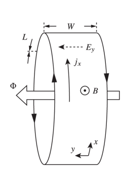
Figure 1: The cylindrical geometry for Laughlin’s argument. Electrons are confined on the cylindrical surface in the presence of a magnetic field $B$ applied perpendicular to the surface. A magnetic flux $\Phi$ is threaded through the hole of the cylinder, and an electric field $E_{y}$ is applied.

A magnetic field $B>0$ is applied in the out-of-plane ($z$) direction. Consider a two-dimensional electron gas ($e<0$) described by a quadratic single-particle Hamiltonian

$$\mathcal{H}=\frac{1}{2m}\left(-i\hbar\bm{\partial}-e\bm{A}\right)^{2},$$ (2)

with the Landau gauge vector potential $\bm{A}=(-By,0)$, which is consistent with the periodic boundary in the $x$ direction. The electronic system has translational invariance in the $x$ direction, and thus eigenstates are labeled by the wave number $k_{x}$. The Hamiltonian (2) has the discrete energy spectrum consisting of the Landau levels,

$$\epsilon_{N}=\hbar\omega_{c}\left(N+\frac{1}{2}\right),$$ (3)

where $N$ is a non-negative integer labeling the Landau levels, and $\omega_{c}=|e|B/m$ is the cyclotron frequency. When the Fermi level lies in the energy gap between the Landau levels $\nu$ and $\nu+1$, that is, the eigenstates up to the Landau level $\nu$ are occupied, the electrons below the Fermi level carry a quantized Hall conductivity as $\sigma_{\text{H}}=\nu e^{2}/2\pi\hbar$. The eigenstate wave functions are given by

$$\phi_{N,k_{x}}(x,y)\propto e^{ik_{x}x}e^{-(y-y_{0})^{2}/2l^{2}}H_{N}(y-y_{0}),$$ (4)

where $l=(\hbar/|e|B)^{1/2}$ is the magnetic length and $H_{N}(y)$ is the Hermite polynomial of degree $N$. The wave functions (4) are localized in the $y$ direction about a point $y_{0}$, and extended in the $x$ direction. Here the localized position $y_{0}$ is uniquely determined by $k_{x}$ via

$$y_{0}=\hbar k_{x}/|e|B.$$ (5)

When the circumference of the cylinder is $L$, the wave number is discretized as $k_{x}=2\pi n/L\,(n\in\mathbb{Z})$ and accordingly, localized positions of the Landau levels take discrete values with the interval $\delta y=2\pi\hbar/|e|BL$.

In Laughlin’s argument, one considers an adiabatic process in which a magnetic flux quantum $\Phi_{0}=2\pi\hbar/|e|$ is threaded through the cylinder. Corresponding change in the vector potential is $\bm{A}\to\bm{A}+(2\pi\hbar/|e|L,0)$. If an electron state is coherent along a closed loop in the $x$ direction, a magnetic flux induces a phase shift by $\psi\to e^{2\pi ix/L}\psi$ that results in a shift of the momentum by $k_{x}\to k_{x}+2\pi/L$. According to (5), the momentum shift is accompanied by an adiabatic shift of the electron position from $y_{0}$ to $y_{0}+\delta y$. Such an adiabatic motion of electrons forced by threading a magnetic flux is the key property in the bulk argument. Note that electrons without coherence undergo trivial changes in their phase factors without any real-space motions. When the length of the cylinder is infinite, or when two boundaries of the cylinder are connected to make a 2-torus, all coherent electrons are shifted to their neighboring positions by one magnetic flux quantum $2\pi\hbar/|e|$, and thus totally the electron state turns back to the original state.

When the electric field is applied in the $y$ direction, an electron localized at $y_{0}$ gains an energy by $\delta E=eE_{y}\delta y$ during a shift to $y_{0}+\delta y$. The charge current is given by $e\bm{j}=\partial\epsilon/\partial\bm{A}$, where $\epsilon$ is the electron energy per unit area. When electrons fill up to the $\nu$th Landau level, the current density is evaluated as

$$ej_{x}=\frac{1}{L\delta y}\frac{\partial E}{\partial A_{x}}\simeq\frac{1}{\delta y}\frac{\delta E}{\Phi_{0}}=\nu\frac{e^{2}}{2\pi\hbar}(-E_{y}),$$ (6)

since all filled Landau levels contribute equally to the Hall current. In (6), a differential is approximated by a difference in the second equality.

III Boundary argument for the quantum Hall effect

In this section, we revisit Laughlin’s argument for the quantum Hall effect in terms of the $c=1$ chiral boundary theory

$$S=\int d^{2}x\,\bar{\psi}i\hbar\left(\partial_{t}+\partial_{x}\right)\psi,$$ (7)

and its intrinsic anomalies. Here and henceforth we set the Fermi velocity as $v_{\text{F}}=1$. The chiral boundary theories cannot exist as an isolated $(1+1)$-dimensional system, and are always accompanied with the higher-dimensional bulk. The quantum anomaly in the U(1) gauge symmetry and the resulting breakdown of the charge conservation are peculiarities in such systems, and are shown to have a close connection with the quantum Hall effect in the bulk. [Here, we consider the sharp boundary with thickness much shorter than the magnetic length $l$ to rule out the possibility of edge reconstructionChamon and Wen (1994). While the subsequent calculations are presented in terms of the simplest edge theory (7), the edge reconstruction is not expected to change the quantum anomaly (the chiral central charge).]

III.1 From perturbative U(1) gauge anomaly

Figure 2: The cylindrical geometry for the boundary picture of Laughlin’s argument. On the cylindrical surface, solid arrows represent electric currents and dashed arrows are the electric field. (a) Electric Hall current in the $x$ direction is induced by an applied voltage $V$. (b) Charge pumping between boundaries as an electric Hall current in the $y$ direction is induced by a temporal change of the magnetic flux $\Phi$.

III.1.1 Charge pumping and anomaly

Consider electrons forming a $\nu=1$ quantum Hall state on the cylindrical geometry [Fig. 2(a)]. The axial length and the circumference of the cylinder are $W$ and $L$, respectively. When a magnetic flux $\Phi_{0}$ is threaded through the cylinder, coherent electrons in the bulk flow adiabatically along the cylinder. At interfaces between boundaries and the bulk, bulk electrons flow into the left boundary, and simultaneously, bulk electrons are supplied by the right boundary.

When we focus on the two boundaries, such a process is interpreted by increase and decrease of the electron numbers in the (1+1)-dimensional electronic systems. The right-(left-)moving chiral boundary fermion mode resides on the left(right) boundary. In the following, we denote “right” and “left” in the subscript of any physical quantities to represent boundary sides, not the moving directions. Combining two chiral modes, the boundary action is given by

$$S_{\text{left}+\text{right}}= \int d^{2}x\,\bar{\psi}(-i)\gamma^{\mu}(\hbar\partial_{\mu}-ieA_{\mu})\psi,$$ (8)

where $\psi=(\psi_{\text{left}},\psi_{\text{right}})$, $\bar{\psi}=\psi^{\dagger}\gamma^{0}$, $\gamma^{0}=i\sigma^{x}$, $\gamma^{1}=\sigma^{y}$ satisfying $\{\gamma^{\mu},\gamma^{\nu}\}/2=\eta^{\mu\nu}=\text{diag}[-1,+1]$, and $\partial_{\mu}=(\partial_{t},\partial_{x})$.

As electrons flow into/from the left/right boundary, the chiral U(1) particle number conservation is violated. This is quantified by the chiral U(1) anomalyBertlmann (1996); Fujikawa and Suzuki (2004) equation

$$\partial_{\mu}j_{5}^{\mu}=-\frac{e}{\pi\hbar}\epsilon^{\mu\nu}\partial_{\mu}A_{\nu},$$ (9)

where $\mu,\nu=t,x$ and $j_{5}^{\mu}=j_{\text{left}}^{\mu}-j_{\text{right}}^{\mu}$ is the axial current composed of the particle current on left and right boundaries. Integrating (9) over the boundary space, one obtains

$$\dot{N}_{\text{left}}-\dot{N}_{\text{right}}=-\frac{e}{\pi\hbar}\dot{\Phi},$$ (10)

where $N_{\text{left(right)}}$ is the total electron number of the left (right) boundary defined by the electron density $j^{0}_{\text{left(right)}}$, and $\Phi$ is the magnetic flux threaded at the center of the boundary circle. On the other hand, the U(1) gauge symmetry of the combination of left and right boundary electrons imposes the conservation of the total electron number $\partial_{t}(N_{\text{left}}+N_{\text{right}})=0$. Therefore, through adiabatically threading a magnetic flux, the electron number changes as

$$\delta N_{\text{left}}=-\delta N_{\text{right}}=-\frac{e}{2\pi\hbar}\Phi.$$ (11)

A relation (11) governing non-conservation of the boundary electron has the same form as the Středa formula for the quantum Hall effectStředa (1982)

$$\sigma_{H}=\nu\frac{e^{2}}{2\pi\hbar}=e\frac{\partial N}{\partial\Phi},$$ (12)

with $\nu=-1$ for the left boundary and $\nu=+1$ for the right one, although (12) considers a magnetic flux $\Phi$ that is applied perpendicularly to the two-dimensional electrons, while that in (11) is threaded through the cylinder. However, the Středa formula (12) and the relation (11) can be identified as follows, provided that the total electrons number $N$ in (12) is completely due to the chiral boundary modes. Consider quantum Hall states on two disks $D_{\text{left}}$ and $D_{\text{right}}$ perpendicular to threaded magnetic flux, which have common boundaries with the cylinder as shown in Fig. 3. Focusing only on the boundary mode, the chiral boundary modes of the $\nu=1$ quantum Hall state on the cylindrical surface are equivalent to those of the $\nu=-1$ quantum Hall state on $D_{\text{left}}$ and the $\nu=1$ quantum Hall state on $D_{\text{right}}$, where, in the latter geometry, electrons on the cylindrical surface are absent. This explains the reason why the boundary electrons obey the Středa formula.

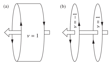
Figure 3: A quantum Hall states on the cylindrical surface have the same boundary electronic modes as those on two disks.

III.1.2 The quantized Hall current induced by the electrostatic potential

Let us now relate (11) to the Hall conductance. When an magnetic flux $\Phi$ is applied, the number of electrons on the left boundary at the electric potential $V$ changes by $\delta N_{\text{left}}$ and that on the right boundary at the electric potential $0$ by $\delta N_{\text{right}}$. The electric potential energy gains by $\delta E_{\text{pot}}=eV\delta N_{\text{left}}$, and, in turn, the total (kinetic) energy of electrons increases by

$$\delta E=-eV\delta N_{\text{left}}.$$ (13)

The electric Hall current is determined by equating the energy supplied by applied voltage and the interaction energy of the electric current with the vector potential resulting from the threaded magnetic flux $A_{x}=\Phi/L$. Thus, using (11), the electronic current is given by

$$eJ_{x}\equiv e\int_{0}^{W}dyj_{x}=\frac{1}{L}\frac{\partial\delta E}{\partial A_{x}}=\frac{e^{2}}{2\pi\hbar}V.$$ (14)

The above argument can be regarded as a boundary picture of Laughlin’s argument on the quantum Hall effect.

Notice that the boundary argument in this subsection cannot tell whether the Hall current flows in the bulk or along the boundary, since it predicts only the total electric Hall current flowing perpendicular to the applied voltage $eJ_{x}\equiv e\int_{0}^{W}dyj_{x}$, i.e., we have computed the Hall conductance, but not the Hall conductivity. Provided that the electric current is uniformly distributed in the bulk, we would conclude that the electric Hall conductivity is quantized as in (6), from (14) (recalling $E_{y}=-V/W$).

Alternatively, one can consistently make an argument based on the electric Hall current flowing along the boundary Halperin (1982); Büttiker (1988). This way of describing the Hall current results from a quantization of the boundary electric current

$$e\frac{\partial j_{\text{bdry}}}{\partial\mu}=\pm\frac{e}{2\pi\hbar},$$ (15)

where $+(-)$ is for the right-(left-)moving chiral fermion. Then the Hall current is calculated solely by a summation of the boundary current on left and right boundaries as

$$J_{x}=j_{\text{left}}+j_{\text{right}}=\frac{\mu_{\text{left}}-\mu_{\text{right}}}{2\pi\hbar}=\frac{e}{2\pi\hbar}V,$$ (16)

which is equivalent to (14). It should be noted, however, the relation (16) does not assert that the Hall current is carried only by the chiral boundary modes. This is because (16) considers only the difference of the electric currents on two boundaries flowing in opposite directions. An absolute value of the boundary electric current is not well-defined for the (1+1)-dimensional Dirac system: it depends on the momentum cutoff $\Lambda$ as

$$j_{\text{left/right}}\equiv\frac{\langle\hat{v}\rangle}{L}\simeq\frac{1}{2\pi}\int_{\pm\Lambda}^{\pm\mu/\hbar}dk=\pm\left(\frac{\mu}{2\pi\hbar}-\frac{\Lambda}{2\pi}\right),$$ (17)

while such a high-frequency regime is not well-defied as the boundary property, and should be attributed to the bulk electronic states. Therefore, the boundary argument in this section does not provide any information about the distribution of the electric Hall current.

III.1.3 The quantized Hall current induced by the time-dependent magnetic flux

Another point to be mentioned is that one can also regard an adiabatic electron transfer between two edges as the electric Hall current flowing in the $y$ direction [Fig. 2(b)], which flows perpendicularly to the Hall current (14) flowing in the $x$ direction [Fig. 2(a)]. The Hall current in this case is induced by a temporal change of the magnetic flux which works as the electric field in the $x$ direction: $E_{x}=-\dot{A_{x}}=-\dot{\Phi}/L$. The voltage between two boundaries is absent in this case ($V=0$), and therefore the bulk electronic states are still in equilibrium during threading the magnetic flux. The electric current density in the bulk is determined by imposing electron number conservation $Lj_{y}-\delta\dot{N}_{\text{left}}=0$ at the left boundary. By using (11), the charge current is related to the electric field as

$$ej_{y}=\frac{e\delta\dot{N}_{\text{left}}}{L}=-\frac{e^{2}}{2\pi\hbar}\frac{\dot{\Phi}}{L}=\frac{e^{2}}{2\pi\hbar}E_{x}$$ (18)

which is equivalent to (14) by rotating $\pi/2$ in the $x$-$y$ plane.

III.2 From global U(1) gauge anomaly

The charge pumping relation (11) derived from the chiral U(1) gauge anomaly can also be derived from another type of anomaly that occurs in the (1+1)-dimensional chiral fermionic system, that is, the global U(1) gauge anomaly.

The U(1) gauge symmetry of the fermionic system refers to invariance under a U(1) gauge transformation

$$\psi(x)\to\psi^{\prime}(x)=e^{2\pi ia(x)}\psi(x).$$ (19)

In order for the fermionic system on a closed one-dimensional space of the circumference $L$ to be invariant, the U(1) gauge transformation must preserve the boundary condition in the spatial direction, which is dictated as $a(L)-a(0)\in\mathbb{Z}$. U(1) gauge transformations satisfying $a(L)-a(0)=0$ can be continuously deformed to the identity transformation ($a(x)=0$), referred to as infinitesimal or small U(1) gauge transformations. The relation (11) is a consequence of an anomaly regarding transformations of this class, which is referred to as the perturbative anomaly. On the other hand, when $a(L)-a(0)=n$ is a nonzero integer, such transformations cannot be continuously deformed to the identity transformation, and are referred to as large U(1) gauge transformations. Threading a magnetic flux is equivalent to a large U(1) gauge transformation, when the magnetic flux is an integer multiple of the flux quantum, $a(L)-a(0)=\Phi/\Phi_{0}$.

Laughlin’s original argument on the quantum Hall state considers a large U(1) gauge transformation for the bulk electronic states induced by threading a magnetic flux quantum. We review the consequence of the same transformation on the boundary theoriesRyu and Zhang (2012); Witten (2016). Consider the (1+1)-dimensional right-moving chiral fermion on a circle with the circumference $L$ given by

$$H=\int_{0}^{L}dx\psi^{\dagger}(x)(-i)\left(\hbar\partial_{x}-ieA_{x}\right)\psi(x),$$ (20)

where the electromagnetic vector potential is induced by the magnetic flux $\Phi$ threaded into the center of the circle, and is related via $A_{x}=\Phi/L$. We incorporate the effect of $A_{x}$ as a twisted boundary condition in the $x$ direction. More generically, we consider the Hamiltonian

$$H=\int_{0}^{L}dx\psi^{\dagger}(-i\hbar\partial_{x})\psi$$ (21)

together with a twisted boundary condition in time as well:

$$\psi(t,x+L)=e^{2\pi i(a-1/2)}\psi(t,x),$$ (22)

$$\psi(t+\hbar\beta,x)=e^{2\pi i(b-1/2)}\psi(t,x).$$ (23)

Parameters $a,b$ play the role of the spatial and temporal flux, specifically, as $a-1/2=\Phi/\Phi_{0}$. In the canonical formalism, the temporal twist is realized by an operation of $\exp(2\pi ibN)$, where $N$ is the total fermion number operator

$$N=\int_{0}^{L}dx\psi^{\dagger}\psi.$$ (24)

Observe that the classical system, as defined by the Hamiltonian (action) and the boundary conditions (22) and (23), is invariant under $a\to a+1$ and $b\to b+1$. This large gauge invariance, however, may be lost once we quantize the theory. In particular, the partition function may acquire an anomalous phase factor (= global U(1) gauge anomaly) under $a\to a+1$ and $b\to b+1$.

The partition function of the (1+1)-dimensional chiral complex fermion (21) with the twisted boundary conditions can be explicitly computed as follows. The fermion field operator is expanded by wave functions satisfying (22) as

$$\psi(x)=\sum_{r\in\mathbb{Z}+a-1/2}e^{2\pi irx/L}\psi_{r},$$ (25)

and the ground state is defined by filling all negative-energy states. When $a\in[-1/2,1/2)$, normal-ordering of the Hamiltonian and the fermion number operator gives

$$H =\frac{2\pi\hbar}{L}\left[\sum_{r\in\mathbb{Z}+a-1/2}r:\psi_{r}^{\dagger}\psi_{r}:-\frac{1}{24}+\frac{a^{2}}{2}\right],$$ (26)

$$N =\sum_{r\in\mathbb{Z}+a-1/2}:\psi_{r}^{\dagger}\psi_{r}:+a,$$ (27)

where extra terms are resulting from the normal-ordering regularized by the Riemann zeta function. Recall that the partition function of the (1+1)-dimensional chiral fermion without twisting ($a=1/2,b=0$) is given by tracing $e^{-\beta H}$ over the Hilbert space satisfying the periodic boundary condition $\psi(x+L)=\psi(x)$. The partition function in the present case is given by

$$Z_{[a,b]} \equiv\text{Tr}\left[e^{-\beta H}e^{2\pi ibN}\right]$$

$$=q^{-1/24+a^{2}/2}e^{2\pi iab}$$

$$\quad\times\prod_{n\in\mathbb{N}}\left(1+q^{n-1/2+a}e^{2\pi ib}\right)\left(1+q^{n-1/2-a}e^{-2\pi ib}\right).$$ (28)

where the tracing refers to the boundary condition (22) and $q=\exp(-2\pi\hbar\beta/L)$.

By inspection, one verifies

$$Z_{[a,b]}=Z_{[a+1,b]}=e^{-2\pi ia}Z_{[a,b+1]}$$ (29)

and hence there is a global U(1) gauge anomaly. From the anomaly, we can read off the charge pumping formula. We normalize the particle number such that the ground state particle number at $a=0$ ($\Phi=-\Phi_{0}/2$) as 0. At $a=0$, by changing the chemical potential $b\to b+1$ one does not earn any phase. On the other hand, at $a\neq 0$, the partition function acquires a non-zero phase factor. This phase is indicative of the change of the ground state fermion number as compared to the fermion number at $a=0$. Since the free energy changes by $\delta F=-2\pi ia/\beta$ during the change of the chemical potential $\delta\mu=2\pi i/\beta$, the particle number is evaluated as $N=-\delta F/\delta\mu=a$. (Note that, from (28), the “imaginary” chemical potential is identified as $\beta\mu=2\pi ib$.) Then,

$$\frac{\partial N}{\partial\Phi}=\frac{1}{\Phi_{0}}\frac{\partial N}{\partial a}=\frac{|e|}{2\pi\hbar},$$ (30)

which is equivalent to the consequence of the perturbative U(1) gauge anomaly (11), although broken symmetries are distinct.

To give a more microscopic view on the global U(1) gauge anomaly, let us follow the spectrum of the Hamiltonian (20) as we change the magnetic flux adiabatically. Under the periodic boundary condition, the eigenfunction is $\phi_{n}(x)=\exp[2\pi inx/L]/\sqrt{L}\,(n\in\mathbb{Z})$, and the corresponding eigenenergy is

$$\epsilon_{n}(\Phi)=\frac{2\pi n\hbar}{L}-\frac{e\Phi}{L}.$$ (31)

After a magnetic flux quantum $\Phi_{0}=2\pi\hbar/|e|$ is threaded, the energy spectra turn back to the original ones by shifting each energy level to the adjacent one ($\epsilon_{n}\to\epsilon_{n+1}$). This implies that the large U(1) gauge transformation leaves the whole electronic energy spectra invariant. However, following gradual change of the energy spectra through threading the magnetic flux, the ground state property changes.

Quantizing the fermion by introducing the anticommutation relation $\{\psi(x),\psi^{\dagger}(x^{\prime})\}=\delta(x-x^{\prime})$, and expanding the fermion operator by the eigenmodes $\psi(x)=\sum_{n}\phi_{n}(x)c_{n}$, the Hamiltonian is rewritten as

$$H=\sum_{n}\epsilon_{n}(\Phi)c_{n}^{\dagger}c_{n}.$$ (32)

If the magnetic flux initially lies in the range $\Phi\in(-\Phi_{0},0)$, the eigenenergy is positive for $n>0$ and negative for $n\leq 0$. The ground state $|0\rangle_{\Phi}$ is made by filling all states with negative eigenenergies, thus the Fermi level lies between $\epsilon_{0}(\Phi)$ and $\epsilon_{1}(\Phi)$. After threading a magnetic flux quantum $\Phi_{0}$, each energy level is shifted as $\epsilon_{n}(\Phi+\Phi_{0})=\epsilon_{n+1}(\Phi)$, and thus the new Fermi level lies between $\epsilon_{1}(\Phi)$ and $\epsilon_{2}(\Phi)$. While the energy spectra are invariant through the magnetic flux change $\Phi\to\Phi+\Phi_{0}$, the number of electrons in the ground state changes by unity $\delta N=1$, since a filled energy level with eigenenergy $\epsilon_{0}(\Phi+\Phi_{0})(=\epsilon_{1}(\Phi))$ goes above the original Fermi level. Let the electron number change be a continuous function of the threaded magnetic flux, the above relation, again, leads to (30).

As shown above, the global U(1) anomaly counts the number of electronic energy levels that traverse the Fermi level during the large U(1) gauge transformation. Within this process, only energy levels close to the Fermi level are concerned. Therefore, as long as the transformation leaves the electronic system invariant at the classical level, the quantized number of traversed energy levels would be unaffected even after small perturbations are added.

IV Boundary argument for the quantized thermal Hall effect

As seen in the previous section, the quantum Hall effect can be explained by anomalies of the (1+1)-dimensional chiral boundary theory. The broken symmetries in these arguments are the invariance under infinitesimal and large U(1) gauge transformations. Here, we extend this boundary argument to the case of the quantized thermal Hall effect. With the help of the Středa formula for the quantized thermal Hall effectNomura et al. (2012)

$$\kappa_{H}=c\frac{\pi k_{\text{B}}^{2}T}{6\hbar}=\frac{\partial S}{\partial\Phi^{\text{g}}},$$ (33)

the relevant symmetry is described by a spacetime transformation given in terms of gravity.

IV.1 Modular transformation

Consider the (1+1)-dimensional system under a static gravitational field $g^{\mu\nu}$. The Středa formula for the quantized thermal Hall effect (33) describes an entropy change induced by the gravitomagnetic flux, which is the gravitational counterpart of the magnetic flux defined by $\Phi^{\text{g}}=A^{\text{g}}_{x}L$. The gravitomagnetic vector potential $A^{\text{g}}_{x}$ is defined by the line element of the Minkowski spacetime

$$ds^{2}=-(dt+A^{\text{g}}_{x}dx)^{2}+dx^{2}.$$ (34)

By the Wick rotation, the line element of the Euclidean spacetime is given by

$$ds^{2}=(dt^{\text{E}}+A^{\text{E}}_{x}dx)^{2}+dx^{2},$$ (35)

where $t^{\text{E}}=it$ is the imaginary time, and $A_{x}^{\text{E}}=iA_{x}^{\text{g}}$ is the gravitomagnetic vector potential in the Euclidean spacetime. In the following, the symbol $t$ is used as the imaginary time in place of $t^{\text{E}}$ for convenience. In the finite-temperature formalism, boundaries of the temporal direction are periodically identified with the period $\hbar\beta=\hbar/(k_{\text{B}}T)$. When the space direction has also the periodic boundary by the period $L$, the spacetime is a 2-torus.

Provided that the gravitomagnetic vector potential $A^{\text{E}}_{x}$ is static, a transformation from a flat spacetime to the one specified by (35) is given by a diffeomorphism

$$(t,x)\to(t+\hbar\beta a^{\text{E}}(x),x),$$ (36)

where $a^{\text{E}}(x)=(\hbar\beta)^{-1}\int_{0}^{x}dx^{\prime}A_{x}^{\text{E}}(x^{\prime})$. Taking into account the fact that the imaginary time is defined modulo $\hbar\beta$, a transformation satisfying $a^{\text{E}}(L)-a^{\text{E}}(0)\in\mathbb{Z}$ leaves the spacetime invariant. Corresponding gravitomagnetic flux $\Phi^{\text{E}}$ is an integer multiple of $\hbar\beta$. A transformation (36) with a nonzero integer $a^{\text{E}}(L)-a^{\text{E}}(0)$ cannot be continuously deformed to the identity transformation. This type of transformations is referred to as large diffeomorphism. Large diffeomorphisms of a torus are referred to as modular transformationsGinsparg (1989); Francesco et al. (1997). Consider a simplest modular transformation given by $\Phi^{\text{E}}_{0}\equiv\hbar\beta$ or $A^{\text{E}}_{x}=\Phi^{\text{E}}_{0}/L$, and a corresponding transformation

$$(t,x)\to(t^{\prime},x^{\prime})=(t+\hbar\beta x/L,x).$$ (37)

After this transformation, periodicity of the spacetime 2-torus is altered from an identification

$$(t,x)\sim(t+\hbar\beta,x)\sim(t,x+L).$$ (38)

to a new identificationGolkar and Sethi (2016)

$$(t,x)\sim(t+\hbar\beta,x)\sim(t+\hbar\beta,x+L),$$ (39)

which is shown in Fig. 4 (a).

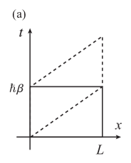
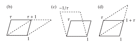
Figure 4: (a) A modular transformation of the spacetime 2-torus induced by threading a gravitomagnetic flux $\Phi^{\text{E}}=\hbar\beta$. A rectangular 2-torus (solid line) is transformed to a sheared-rectangular 2-torus (dashed line). Boundaries on left and right, and those on top and bottom are identified, respectively. The modular group is generated by (b) $T:\tau\to\tau+1$, and (c) $S:\tau\to-1/\tau$. (d) Another basic transformation can be composed by $TST:\tau\to\tau/(1+\tau)$.

The transformation (37) represents a sequence of prescriptions composed of, cutting the spacetime torus by a loop along the temporal direction, twisting one of the edges by $\hbar\beta$, and gluing two edges to make a 2-torus again. Notice that the unit of the gravitomagnetic flux inducing a modular transformation is $\Phi^{\text{g}}_{0}=-i\hbar\beta$, while the unit of the magnetic flux bringing about a large U(1) gauge transformation is the magnetic flux quantum $\Phi_{0}=2\pi\hbar/|e|$.

Before moving on, we briefly review the concept of the modular groupFrancesco et al. (1997). The spacetime 2-torus is defined by periodicities, and thus is the quotient space of the two-dimensional Euclidean space $\mathbb{R}^{2}$ by a two-dimensional lattice spanned by two linearly-independent lattice vectors. When the torus is defined on the complex plane $\mathbb{C}$ by, e.g. $z=x+it$, the lattice vectors are represented by two complex numbers $\omega_{1},\omega_{2}\in\mathbb{C}$ as

$$(t,x)\sim(t+\text{Im}[\omega_{1(2)}],x+\text{Re}[\omega_{1(2)}]).$$ (40)

As in the description of crystals, there is an ambiguity in choice of the lattice vectors. Another set of lattice vectors given by a transformation

$$\begin{pmatrix}\omega_{2}^{\prime}\\ \omega_{1}^{\prime}\end{pmatrix}=\begin{pmatrix}a&b\\ c&d\end{pmatrix}\begin{pmatrix}\omega_{2}\\ \omega_{1}\end{pmatrix}$$ (41)

satisfying $ad-bc=1\,(a,b,c,d\in\mathbb{Z})$, spans the same lattice, since the transformation matrix is invertible. The matrix in (41) leaves the area spanned by two lattice vectors invariant, and forms a group $S\!L(2,\mathbb{Z})$ of $2\times 2$ integer-valued matrices with unit determinant.

Thanks to the conformal invariance that the linearized form of the gapless boundary fermion (7) possesses, physical properties on a torus should be invariant up to scaling, and thus be dependent only on the ratio of two periods $\tau=\omega_{2}/\omega_{1}$, which is referred to as the modular parameter. Redefinition of lattice vectors (41) transforms the modular parameter as

$$\tau^{\prime}=\frac{a\tau+b}{c\tau+d},$$ (42)

which forms a group $PS\!L(2,\mathbb{Z})=S\!L(2,\mathbb{Z})/\mathbb{Z}_{2}$, referred to as the modular group. Here $\mathbb{Z}_{2}$ in the modular group is due to the fact that inverting the signs of $a,b,c,d$ leaves the transformation unchanged. The modular group is known to be generated by two operations $T:\tau\to\tau+1$ and $S:\tau\to-1/\tau$ [Fig. 4 (b) and (c)].

Here, we apply the above framework to our situation. The lattice vectors of the rectangular spacetime torus (38) are assigned as $\omega_{1}=L$ and $\omega_{2}=i\hbar\beta$, and corresponding lattice vectors of the sheared rectangular spacetime torus (39) are $\omega_{1}=L+i\hbar\beta$ and $\omega_{2}=i\hbar\beta$. Defining the ratio of spatial and temporal periods by $\alpha=\hbar\beta/L$, the modular parameter is changed from $\tau=i\alpha$ to $\tau^{\prime}=i\alpha/(1+i\alpha)$ during the gravitomagnetic flux $\Phi^{\text{E}}_{0}$ is threaded. This process is a modular transformation given by $TST:\tau\to\tau/(1+\tau)$ [Fig. 4 (d)].

Notice that, in the above context, we have encoded the gravitomagnetic flux into the change of the lattice vectors that span the spacetime torus, not into the change of the metric with which the fermionic kinetic action is defined. These two interpretations are equivalent, at least, when the gravitomagnetic flux is uniform in the whole spacetime (see for details in appendix A). With this in mind, we study, throughout this paper, the fermionic action on the flat spacetime under the boundary condition specified by the threaded magnetic and gravitomagnetic fluxes.

IV.2 Free energy pumping and global diffeomorphism anomaly

In this section, the breakdown of the modular invariance, that is, the global diffeomorphism anomalyWitten (1985); Ryu and Zhang (2012); Witten (2016); Golkar and Sethi (2016), of the (1+1)-dimensional edge theory of the quantum Hall systems is reviewed, and is shown to account for the quantized thermal Hall effect.

For our calculation of the global diffeomorphism anomaly, we again employ the chiral massless Dirac fermion theory (21). It should be stressed that this theory (21) enjoys an exact conformal (and/or Lorentz) symmetry, which makes the following calculations rather transparent. In contrast, the (realistic) edge theory of the quantum Hall boundary realizes the conformal symmetry only approximately at low energies. Our rationale of assuming the exact conformal symmetry is that we focus on the renormalization group fixed point, which, irrespective of microscopic details, is described by a scale invariant field theory. For edge theories which are not quite at a renormalization group fixed point, we invoke the usual ’t Hooft anomaly matching, i.e., the calculation of quantum anomalies should not depend on what energy/length scale is chosen for the calculation. This should be contrasted with our calculation of the large U(1) gauge anomaly and the quantized Hall conductance: The large U(1) gauge invariance is an exact symmetry of the system at all scales. On the other hand, in the thermal/gravitational case, at least technically, our calculation of the global gravitational anomaly (presented below) relies on an emergent conformal symmetry at low energies. We leave it as a future problem whether or not the reliance on the conformal symmetry can be relaxed or completely removed. (See, however, Ref. Kitaev, 2006, where it was attempted to give the definition of the chiral central charge without assuming conformal symmetry.)

The global diffeomorphism anomaly can be read off from the partition function. In addition to the modular parameter $\tau$ that characterizes the base spacetime manifold, one needs to specify the boundary condition of the fermion defined on it. The boundary condition is, in general, defined for two periods by

$$\psi(t+\text{Im}[\omega_{1}],x+\text{Re}[\omega_{1}])=e^{2\pi i(a-1/2)}\psi(t,x),$$ (43)

$$\psi(t+\text{Im}[\omega_{2}],x+\text{Re}[\omega_{2}])=e^{2\pi i(b-1/2)}\psi(t,x).$$ (44)

The boundary conditions for the fermion on the spacetime torus without the gravitomagnetic flux (38) is given by

$$\begin{aligned} &\psi(t,x+L)=\psi(t,x),\\ &\psi(t+\hbar\beta,x)=-\psi(t,x),\end{aligned}$$ (45)

which corresponds to $\tau=i\alpha$ and $[a,b]=[\frac{1}{2},0]$. On the other hand, the boundary condition on a torus with the gravitomagnetic flux $\Phi^{\text{E}}_{0}$ specified by (39) is

$$\begin{aligned} &\psi(t+\hbar\beta,x+L)=-\psi(t,x),\\ &\psi(t+\hbar\beta,x)=-\psi(t,x),\end{aligned}$$ (46)

which corresponds to $\tau=i\alpha/(1+i\alpha)$ and $[a,b]=[0,0]$. If the fermionic system is invariant under the modular transformation, the partition function should be unchanged during the transformation. This is not true for the present case since there is an anomaly regarding the modular invariance.

The partition function of the (1+1)-dimensional chiral complex fermion (21) with the boundary condition specified by the modular parameter $\tau=\tau_{1}+i\tau_{2}\alpha$ and $[a,b]$ is calculated, in much the same way as in Sec. III.2:

$$Z_{[a,b]}(\tau)\equiv\text{Tr}\left[e^{-\tau_{2}\beta H}e^{i\tau_{1}LP/\hbar}e^{2\pi ibN}\right]$$

$$=q^{-1/24+a^{2}/2}e^{2\pi iab}$$

$$\quad\times\prod_{n\in\mathbb{N}}\left(1+q^{n-1/2+a}e^{2\pi ib}\right)\left(1+q^{n-1/2-a}e^{-2\pi ib}\right),$$ (47)

where $P=H$ (we have set the Fermi velocity as $v_{\text{F}}=1$) and $q=e^{2\pi i\tau}$. Under the modular transformation $TST:\tau\to\tau/(1+\tau)$, the partition function of the boundary fermion is transformed asGinsparg (1989); Francesco et al. (1997)

$$Z_{[\frac{1}{2},0]}(i\alpha)\to Z_{[0,0]}(i\alpha/(1+i\alpha))$$

$$=e^{-i\pi/12}Z_{[0,\frac{1}{2}]}(-1/(1+i\alpha))$$

$$=e^{-i\pi/12}Z_{[\frac{1}{2},0]}(1+i\alpha)$$

$$=e^{i\pi/12}Z_{[\frac{1}{2},0]}(i\alpha).$$ (48)

A contribution due to the global diffeomorphism anomaly appears as an extra phase factor $e^{i\pi/12}$. Therefore an extra imaginary free energy $\delta F=-i\pi/12\beta$ is generated during this process. Since a real gravitomagnetic flux $\Phi^{\text{E}}_{0}=\hbar\beta$ in the Euclidean spacetime corresponds to an imaginary gravitomagnetic flux $\Phi^{\text{g}}_{0}=-i\hbar\beta$ in the Minkowski spacetime, a free energy change induced by the gravitomagnetic flux is formulated as

$$\frac{\partial F}{\partial\Phi^{\text{g}}}\simeq\frac{\delta F}{\Phi^{\text{g}}_{0}}=\frac{\pi k_{\text{B}}^{2}T^{2}}{12\hbar},$$ (49)

where in the first equality, a differential is approximately given by a difference as in the case of the global U(1) gauge anomaly (30). An indication of the relation (49) is that the (1+1)-dimensional gapless fermionic system loses or gains free energy depending on its central charge, by threading the gravitomagnetic flux into the one-dimensional space loop.

The free energy (49) has been derived and discussed in the context of the anomaly-related transport phenomena . In particular, Golkar and Sethi Golkar and Sethi (2016) discussed the free energy (49) by using the global gravitational anomaly. (The same free energy was also obtained in Ref. Nakai et al., 2016 – see discussion below.) It should be noted however that this method of determining an effective free energy from the global anomaly suffers from an ambiguity. The free energy change can be determined only up to an integer multiple of $2\pi$,

$$\delta F=(-i/\beta)(\pi/12+2\pi n)\quad(n\in\mathbb{Z}),$$ (50)

since the logarithm of the extra phase factor $e^{i\pi/12}$ can be determined up to an integer multiple of $2\pi i$ Chowdhury and David (2016). Nevertheless, the ambiguity can be removed by requiring the consistency with the perturbative gravitational anomaly, and the boundary thermal conductivity Cappelli et al. (2002); Chowdhury and David (2016) leading to the free energy (49).

Observe the same ambiguity does exist for the case of the global U(1) gauge anomaly: The global anomaly (the anomalous phase acquired by the partition function under large U(1) gauge transformations) is determined only up to an integer multiple of $2\pi$. Once again, matching the global anomaly with the perturbative U(1) gauge anomaly removes the ambiguity. It should be also noted that, for the case of the global U(1) gauge anomaly, the situation is slightly better as there are two compact adiabatic parameters, $a$ and $b$, that we can change. While the anomalous phase $\exp(2\pi ia)$ under $b\to b+1$ has an ambiguity, demanding that the phase is a continuous function of $a$, one can read off the Hall conductance from the derivative of $\ln[\exp 2\pi ia]$ with respect to $a$, which is free from the ambiguity. On the other hand, for the gravitational case, we have only one compact variable $\tau$. We thus need to resort on consistency with the perturbative gravitational anomaly to fix the ambiguity.

If we need to fix the ambiguity with the help of the perturbative anomaly, one may wonder why we need to rely on the global anomaly in the first place. However, as noted previously Stone (2012), deriving the thermal response by using the perturbative gravitational anomaly is not obvious, as one needs to relate the gravitational response to the thermal response by using Luttinger’s trickLuttinger (1964). On the other hand, as we will demonstrate in the following, the thermal response appears more naturally when we consider the global diffeomorphism anomaly.

A direct consequence of (49) is the Středa formula for the quantized thermal Hall effect. Using a thermodynamic relation $\delta S=-\partial\delta F/\partial T$, the Středa formula is derived as

$$\frac{\delta S}{\Phi^{\text{g}}_{0}}=-\frac{\pi k_{\text{B}}^{2}T}{6\hbar}=\kappa_{H}(c=-1),$$ (51)

where $\kappa_{H}(c)$ represents the quantized thermal Hall conductivity for the chiral central charge $c$. (51) is the Středa formula for the quantized thermal Hall effect in the $\nu=-1$ quantum Hall system, and is quite analogous to (12) for the quantum Hall effect led by the U(1) gauge anomaly.

Although the free energy (49) is a functional only of the gravitomagnetic vector potential $A^{\text{g}}_{x}$:

$$F[A^{\text{g}}_{x}]=\frac{\pi k_{\text{B}}^{2}T^{2}}{12\hbar}\int_{0}^{L}dxA^{\text{g}}_{x},$$ (52)

one can deduce a form of the free energy when a gravitational potential field $\sigma$ is additionally present. The metric is given by

$$ds^{2}=e^{-2\sigma}\left(dt+iA_{x}^{\text{g}}dx\right)^{2}+dx^{2}.$$ (53)

Thus including a gravitational potential is reduced to changes $\beta\to e^{-\sigma}\beta$ and $A_{x}^{\text{g}}\to e^{-\sigma}A_{x}^{\text{g}}$. The global diffeomorphism anomaly in this new metric is read off from the free energy change $\delta F=-i\pi e^{\sigma}/12\beta$ induced by $\Phi^{\text{g}}=-i\hbar e^{-\sigma}\beta$, which results in the free energy as a functional of $\sigma$ and $A^{\text{g}}_{x}$. Expanding with respect to the gravitational potential as

$$F[\sigma,A^{\text{g}}_{x}] =\frac{\pi k_{\text{B}}^{2}T^{2}}{12\hbar}\int_{0}^{L}dxe^{2\sigma}A^{\text{g}}_{x}$$

$$=F[A^{\text{g}}_{x}]+F^{(1)}[\sigma,A^{\text{g}}_{x}]+O(\sigma^{2}),$$ (54)

the zeroth-order term is given in (52), while the first-order term

$$F^{(1)}[\sigma,A^{\text{g}}_{x}]=\frac{\pi k_{\text{B}}^{2}T^{2}}{6\hbar}\int_{0}^{L}dx\,\sigma A^{\text{g}}_{x},$$ (55)

is equivalent to the boundary free energy derived by the authors in a previous paperNakai et al. (2016).

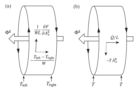
Figure 5: A setup for Laughlin’s argument on the quantized thermal Hall effect from the boundary theory. On the cylindrical surface, solid arrows represent thermal currents and dashed arrows represent temperature gradients. (a) Left and right boundaries are in contact with heat baths and are in thermal equilibrium at temperature $T_{\text{left}}$ and $T_{\text{right}}$, respectively. The thermal Hall current is induced by the temperature difference between boundaries. (b) Two boundaries are in thermal equilibrium at the same temperature $T$. A transferred heat between boundaries as a thermal Hall current is induced by a temporal change of the gravitomagnetic flux $\Phi^{\text{g}}$.

IV.3 The quantized thermal Hall current induced by the temperature gradient

Now we are ready to extend Laughlin’s argument using the relation in the previous subsection (49). Consider a geometry shown in Fig. 5(a). The bulk electrons form a quantum Hall state with the Chern number $\nu=1$. Left and right boundaries are in the thermal equilibrium at temperature $T_{\text{left}}$ and $T_{\text{right}}$, respectively, by contacting them with heat baths. The quantum Hall state on the cylindrical surface is assumed to have an energy gap much larger than both boundary temperatures so that the electronic excitations are suppressed in the bulk.

The thermal Hall current can be read off by equating the free energy generated at the boundaries as a result of the global diffeomorphism anomaly (49), and an interaction energy of the thermal current with the gravitomagnetic vector potential induced by the gravitomagnetic flux. A free energy generated at left and right boundaries is given, respectively, by

$$\delta F_{\text{left}}=\frac{\pi k_{\text{B}}^{2}T^{2}_{\text{left}}}{12\hbar}\Phi^{\text{g}},\quad\delta F_{\text{right}}=-\frac{\pi k_{\text{B}}^{2}T^{2}_{\text{right}}}{12\hbar}\Phi^{\text{g}},$$ (56)

and thus the change of the total free energy by

$$\delta F\equiv\delta F_{\text{left}}+\delta F_{\text{right}}=\frac{\pi k_{\text{B}}^{2}}{12\hbar}\left(T^{2}_{\text{left}}-T^{2}_{\text{right}}\right)\Phi^{\text{g}}.$$ (57)

When the temperature difference between two boundaries is sufficiently small compared with boundary temperatures themselves ($|T_{\text{left}}-T_{\text{right}}|\ll T_{\text{left(right)}}$), one obtains

$$\delta F\simeq\frac{\pi k_{\text{B}}^{2}\bar{T}}{6\hbar}(T_{\text{left}}-T_{\text{right}})\Phi^{\text{g}},$$ (58)

where $\bar{T}$ is the average temperature between $T_{\text{left}}$ and $T_{\text{right}}$. The thermal current (energy current) couples to the gravitomagnetic field, and is derived from this free energy as

$$\int^{W}_{0}dy\,j_{x}^{T}=\frac{1}{L}\left(\frac{\partial\delta F}{\partial A_{x}^{\text{g}}}\right)=\frac{\pi k_{\text{B}}^{2}\bar{T}}{6\hbar}(T_{\text{left}}-T_{\text{right}}),$$ (59)

which is the quantized thermal Hall effect with the thermal Hall conductance $\pi k_{\text{B}}^{2}\bar{T}/6\hbar$ for the Chern number $\nu=1$. Notice that the boundary argument presented above is free from the fictitious temperature gradient in terms of gravity, that is, Luttinger’s trickLuttinger (1964) using the Tolman-Ehrenfest relation $-T^{-1}\nabla_{x}T=-\nabla_{x}\sigma$ by the gravitational potential $\sigma$.

As a result, when two sides of the quantum Hall boundaries contact with heat baths with different temperature, a thermal current flows parallel to the boundaries, and the thermal Hall conductance is quantized by the central charge of the chiral boundary modes, which, in this case, is equivalent to the bulk Chern number. However it should be noted that the boundary argument cannot tell whether the thermal Hall current flows in the bulk or along the boundary, due to the same reason as we mentioned in Sec. III.1.2 for the quantum Hall effect. The relation (59) tells us about the total thermal Hall current $L^{-1}\partial\delta F/\partial A_{x}^{\text{g}}$ integrated over the section of the Hall bar geometry. For example, one can also explain the thermal Hall effect solely by the boundary thermal current. The thermal current of the (1+1)-dimensional fermion is evaluated as

$$\frac{\partial j^{T,\text{bdry}}}{\partial T}=(c-\bar{c})\frac{\pi k_{\text{B}}^{2}T}{6\hbar},$$ (60)

which is related to a perturbative gravitational anomaly Cappelli et al. (2002). Although the relation (60) is enough to show the quantized thermal Hall effect when two boundaries have different temperature, we cannot conclude, from this relation, that the thermal Hall current flows only near the boundary. This is because the absolute value of a thermal current flowing along the boundary cannot be determined.

The boundary argument presented in this section, and the similar one in the previous section for the quantum Hall effect, rely on the presence of the chiral massless fermionic mode on the boundary and the gapful bulk. The presence of the chiral massless fermion is robust against perturbations including disorders and interaction as long as the bulk energy gap is large enough compared with perturbations. Furthermore, the boundary mode is robust against perturbations on the boundary due to chirality. However, unlike the case of the quantum Hall effect where the large U(1) gauge invariance and quantization of electric responses are exact for the chiral boundary modes, the thermal Hall coefficient is not necessarily quantized, in a strict meaning, due to the breakdown of the scale invariance by microscopic details of the model.

IV.4 The quantized thermal Hall current induced by the time-dependent gravitomagnetic flux

Following the discussion of the quantum Hall effect in Sec. III.1.3, we now discuss the possibility of regarding a heat transfer between two boundaries as the quantized thermal Hall current [Fig. 5(b)]. When the both boundaries are in equilibrium at the same temperature $T$, the total free energy conserves due to (56), which indicates a heat is transferred between boundaries by threading a gravitomagnetic flux. The amount of the transferred heat is evaluated as $\delta Q=T\delta S=-Td\delta F/dT$. By imposing the continuity equation of the heat at the left boundary, a thermal current in the bulk is determined by $Lj^{T}_{y}-\delta\dot{Q}=0$. Therefore

$$j^{T}_{y}=\frac{\delta\dot{Q}}{L}=-\frac{T}{L}\frac{d\delta\dot{F}}{dT}=\frac{\pi k_{\text{B}}^{2}T^{2}}{6\hbar}(-\dot{A}_{x}^{\text{g}}).$$ (61)

This expression indicates that, if we recognize the time derivative of the gravitomagnetic vector potential as a fictitious temperature gradient by $-T^{-1}\nabla_{x}T=-\dot{A}^{\text{g}}_{x}$, a heat transfer in the $y$ direction between two boundaries can also be regarded as a quantized thermal Hall current. Notice that, in addition to the Tolman-Ehrenfest relation $-T^{-1}\nabla_{x}T=-\nabla_{x}\sigma$, a gravitational expression of a temperature gradient should be given by

$$-T^{-1}\nabla_{x}T=-\nabla_{x}\sigma-\dot{A}^{\text{g}}_{x},$$ (62)

which is analogous to the expression of the electric field in terms of the electric potential $\phi$ and the vector potential $A$ in electromagnetism: $E_{x}=-\nabla_{x}\phi-\dot{A}_{x}$. A similar expression has been employed in evaluation of the thermal current Tatara (2015), although definition of the vector potential in this literature is different from ours.

V Bulk argument for the quantized thermal Hall effect

In this final section, we will develop yet another argument for the quantized thermal Hall effect following the spirit of the original Laughlin’s argument presented in Sec. II. We will apply the modular transformation (37) to the bulk electronic states forming the Landau levels, and examine an adiabatic transport induced by the modular transformation. As in the original Laughlin’s argument, our discussion here relies on and is limited to single-particle eigenfunctions of the Landau levels, but gives a complementary view to the boundary argument presented in Sec. IV.

V.1 Modular transformations for bulk wavefunctions

Consider the Fourier modes of the fermion field on the Euclidean (2+1)-dimensional spacetime labeled by the fermionic Matsubara frequency $\omega_{n}=2\pi(n+1/2)/\hbar\beta\,(n\in\mathbb{Z})$ and the momentum $k_{x}=2\pi l/L\,(l\in\mathbb{Z})$,

$$\tilde{\psi}(i\omega_{n},k_{x},y)=\frac{1}{\sqrt{\beta L}}\int d^{2}xe^{i\omega_{n}t-ik_{x}x}\psi(t,x,y).$$ (63)

Consider a continuous diffeomorphism of the base manifold as a function of the threaded gravitomagnetic flux. Boundary conditions (45) and (46) are continuously connected by an intermediate boundary condition

$$\begin{aligned} &\psi(t+s\hbar\beta,x+L,y)=e^{-s(2m+1)\pi i}\psi(t,x,y),\\ &\psi(t+\hbar\beta,x,y)=-\psi(t,x,y),\end{aligned}$$ (64)

where $m$ is an arbitrary integer and $s=\Phi^{\text{E}}/\Phi^{\text{E}}_{0}\in[0,1]$. The fermion field satisfying (64) can be expanded by plain waves $\exp[-i\omega_{n}(t-s\hbar\beta x/L)+ik_{x}^{(s)}x]$ where $k_{x}^{(s)}=2\pi l/L-s(2m+1)\pi/L\,(l\in\mathbb{Z})$. The modular transformation (37) transforms a Fourier mode continuously as

$$\tilde{\psi}(i\omega_{n},k_{x}^{(0)},y)$$

$$\to\frac{1}{\sqrt{\beta L}}\int d^{2}x\exp\left[i\omega_{n}\left(t-\frac{s\hbar\beta x}{L}\right)-ik_{x}^{(s)}x\right]\psi(t,x,y)$$

$$=\frac{1}{\sqrt{\beta L}}\int d^{2}x\exp\left[i\omega_{n}t-i\left(k_{x}^{(s)}+\frac{s\omega_{n}\hbar\beta}{L}\right)x\right]\psi(t,x,y)$$

$$=\tilde{\psi}(i\omega_{n},k_{x}^{(0)}+s(n-m)2\pi/L,y),$$ (65)

At $s=1$, the momentum is changed as $k_{x}\to k_{x}+(n-m)2\pi/L$. Thus, by expanding the fermion field with respect to the imaginary time, the modular transformation results in a frequency-dependent momentum shift. One can remove an integer $m$ by threading magnetic flux quanta. This prescription does not affect the following argument, since the magnetic flux does not induce the thermal Hall current. For later convenience, we consider twice the unit of the modular transformation ($s=2$), and the momentum is shifted as $k_{x}\to k_{x}+(2n+1)2\pi/L$. As explained in Sec. II, a momentum shift in the quantum Hall state is accompanied with an adiabatic shift of the center of mass of wavefunctions, which can be read off from (5) as

$$y\to y+(2n+1)\delta y,$$ (66)

where $\delta y=2\pi\hbar/|e|BL$. Thus, by threading the gravitomagnetic flux $2\Phi^{\text{E}}_{0}$, bulk quantum Hall electronic states with the Matsubara frequency $\omega_{n}$ are adiabatically transferred from their original localized positions to their $(2n+1)$th neighboring positions. This should be contrasted with the original Laughlin’s argument for the quantum Hall effect, where, after threading a magnetic flux quantum $\Phi_{0}$, all electronic states are equally shifted to their neighboring positions. When the quantum Hall system is in a thermal equilibrium, the gravitomagnetic-flux threading leaves the whole electronic system unchanged.

V.2 The quantized thermal Hall current induced by the static gravitational potential

Consider the situation that a temperature gradient is applied uniformly in the bulk. Local temperature is defined through Luttinger’s trick using the Tolman-Ehrenfest relation $T(y)=\bar{T}e^{\sigma(y)}$, where $e^{-2\sigma}=g_{00}$, and $\bar{T}$ is a reference temperature independent of location, and simultaneously serves as a bulk temperature when $\sigma(y)$ is small enough. Here we focus on a specific position $y_{0}$ of a localized position of the Landau level wave function determined by (5). The $j$th neighboring localized position deviated from $y_{0}$ is denoted by $y_{j}=y_{0}+j\delta y$. Also, we define the local temperature at a position $y_{j}$ by $T_{j}\equiv T(y_{j})$, and its inverse by $\beta_{j}\equiv(k_{\text{B}}T_{j})^{-1}$.

In order to capture qualitatively the changes in physical quantities induced by an adiabatic shift (66), we consider the partition function of the bulk quantum Hall states under a uniform temperature gradient. We assume that the position-dependent temperature is represented in the partition function by the upper bound of the imaginary time integral as $\beta(y)=(k_{\text{B}}T(y))^{-1}$. Then the action and the partition function are given by

$$S =\int d\bm{x}\int_{0}^{\hbar\beta(y)}dt\,\bar{\psi}(t,\bm{x})\left(\hbar\partial_{t}+\mathcal{H}-\mu\right)\psi(t,\bm{x}),$$

$$Z =\int\mathcal{D}\bar{\psi}\mathcal{D}\psi\,\exp(-S/\hbar),$$ (67)

where $\bm{x}=(x,y)$, and $\mathcal{H}$ is the Hamiltonian of the bulk two-dimensional electron system under a perpendicular magnetic field, defined in (2). The fermion field operator is expanded by the eigenstate wavefunctions of the Landau levels (4) as

$$\psi(t,\bm{x})=\sum_{N,k_{x}}\phi_{N,k_{x}}(\bm{x})\frac{1}{\sqrt{\beta_{j}}}\sum_{n}e^{-i\omega_{n}(y_{j})t}\psi_{n,N,k_{x}},$$ (68)

$$\bar{\psi}(t,\bm{x})=\sum_{N,k_{x}}\phi_{N,k_{x}}^{\ast}(\bm{x})\frac{1}{\sqrt{\beta_{j}}}\sum_{n}e^{i\omega_{n}(y_{j})t}\bar{\psi}_{n,N,k_{x}},$$ (69)

where $\omega_{n}(y_{j})=(2n+1)\pi/\hbar\beta_{j}$, and $\beta_{j}$ is uniquely determined by $k_{x}$. Then the action becomes

$$S/\hbar=\sum_{n,N,k_{x}}\bar{\psi}_{n,N,k_{x}}\left(-i\hbar\omega_{n}(y_{j})+\epsilon_{N}-\mu\right)\psi_{n,N,k_{x}},$$ (70)

where $\epsilon_{N}$ is the $N$th Landau level energy (3), and we have used the fact that the Landau level wavefunction $\phi_{N,k_{x}}$ is localized about the position $y_{j}$. Thus we decompose the partition function by the momentum $k_{x}$ and calculate the path integral part by part as

$$Z =\prod_{n,N,j}\beta_{j}\left(-i\hbar\omega_{n}(y_{j})+\epsilon_{N}-\mu\right),$$ (71)

where the summation over the momentum $k_{x}$ is replaced by that over the index of the localized position $j$. The total free energy is given by

$$F =-\sum_{n,N,j}\beta_{j}^{-1}\ln\left[\beta_{j}\left(-i\hbar\omega_{n}(y_{j})+\epsilon_{N}-\mu\right)\right]\equiv\sum_{n,j}F_{n}(y_{j}).$$ (72)

Let us now focus on the local free energy at position $y_{0}$. A local change of the bulk free energy can be evaluated by collecting parts of the partition function localized at $y_{0}$ before and after threading the gravitomagnetic flux. Before threading the gravitomagnetic flux, the local free energy at $y_{0}$ is given by

$$F(y_{0}) =\sum_{n}F_{n}(y_{0}).$$ (73)

Consider threading a uniform gravitomagnetic flux $\Phi^{\text{E}}$. As we showed in Sec. V.1, when the flux $\Phi^{\text{E}}=2\hbar\beta_{j}$ is threaded, a Fourier mode with $(\omega_{n}(y_{j}),k_{x})$, which is localized at $y_{j}$, is adiabatically changed to a mode with $(\omega_{n}(y_{j}),k_{x}+(2n+1)2\pi/L)$. As for the local free energy at $y_{0}$, a part of the free energy with $\omega_{n}(y_{0})$ originally at $y_{0}$ flows out to $y_{2n+1}$ when $\Phi^{\text{E}}=2\hbar\beta_{0}$. On the other hand, the free energy with $\omega_{n}(y_{-(2n+1)})$ at $y_{-(2n+1)}$ flows into $y_{0}$ when $\Phi^{\text{E}}=2\hbar\beta_{-(2n+1)}$ (Fig. 6).

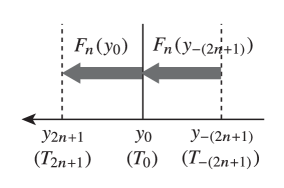
Figure 6: Transferred components of the bulk free energy in a quantum Hall state induced by the gravitomagnetic flux $\Phi^{g}=-2i\hbar\beta$.

Then the local free energy change at $y_{0}$ is given by

$$\delta F(\Phi^{\text{g}};y_{0}) =i\Phi^{\text{g}}\sum_{n}\left[\frac{F_{n}(y_{-(2n+1)})}{2\hbar\beta_{-(2n+1)}}-\frac{F_{n}(y_{0})}{2\hbar\beta_{0}}\right],$$ (74)

where we assume $\delta F$ to be a smooth function of the gravitomagnetic flux $\Phi^{\text{g}}$.

The right-hand side of (74) is evaluated as follows. Assuming the temperature gradient is relatively small, one obtains

$$\delta F(\Phi^{\text{g}};y_{0})\simeq i\Phi^{\text{g}}\sum_{n}\left(T_{-(2n+1)}-T_{0}\right)\left(\frac{\partial}{\partial T}\frac{F_{n}(y)}{2\hbar\beta}\right)_{y_{0}}$$

$$=i\Phi^{\text{g}}\delta T\sum_{n}(2n+1)\frac{\partial}{\partial T}\sum_{N}\frac{\ln\left[\beta\left(-i\hbar\omega_{n}+\epsilon_{N}-\mu\right)\right]}{2\hbar\beta^{2}}$$

$$=-\frac{\Phi^{\text{g}}\delta T}{2\pi\hbar}\sum_{N}\frac{\partial}{\partial T}\beta^{-1}\sum_{n}(-i\hbar\omega_{n})\ln\left[\beta\left(-i\hbar\omega_{n}+\epsilon_{N}-\mu\right)\right],$$ (75)

where $\delta T=T_{j+1}-T_{j}$ is the difference of the temperature between neighboring localized positions. Evaluating the Matsubara summation, one obtains

$$\sum_{n}(-i\hbar\omega_{n})\ln\left[\beta\left(-i\hbar\omega_{n}+\epsilon_{N}-\mu\right)\right]=G\left(\epsilon_{N}-\mu\right),$$ (76)

where $G(z)$ is the integral of $\beta z/(e^{\beta z}+1)$. At low temperatures, $G(z)$ is expanded with respect to the temperature by the Sommerfeld expansion as

$$G(z)=\int_{\infty}^{z}dz^{\prime}\frac{\beta z^{\prime}}{e^{\beta z^{\prime}}+1}=\theta(-z)\left(\frac{\beta z^{2}}{2}-\frac{\pi^{2}}{6\beta}\right)+O(T^{3}),$$ (77)

where $\theta$ is the Heaviside step function. The local free energy change is then given by

$$\delta F(\Phi^{\text{g}};y_{0})=\nu\frac{\pi k_{\text{B}}^{2}T_{0}}{6\hbar}\Phi^{\text{g}}\delta T,$$ (78)

where $\nu$ is the number of filled Landau levels and is equal to the total Chern number of filled energy levels. Since each localized position is separated by an interval $\delta y$, the bulk thermal current is given by

$$j_{x}^{T}=\frac{1}{L\delta y}\frac{\partial\delta F(\Phi^{\text{g}};y_{0})}{\partial A_{x}^{\text{g}}}=\nu\frac{\pi k_{\text{B}}^{2}T_{0}}{6\hbar}\nabla_{y}T,$$ (79)

where $\delta T=(\nabla_{y}T)\delta y$ and $\Phi^{\text{g}}=LA_{x}^{\text{g}}$ are used. The above relation is the quantized thermal Hall effect in the quantum Hall state with the Chern number $\nu$. (79) satisfies the Wiedemann-Franz law with the Laughlin’s original result (6). The above argument quantitatively describes how a thermal Hall current can flow adiabatically in a gapped bulk.

VI Conclusion

We studied the generalization of Laughlin’s magnetic-flux-threading argument to the quantized thermal Hall effect in terms of gravity, from the perspective of both bulk and boundary theories.

The boundary argument reveals that the global diffeomorphism anomaly accounts for the quantized thermal Hall effect. More precisely, we formulated, quantitatively, the responses of the chiral boundary modes against the gravitomagnetic flux, by making use of the global diffeomorphism anomaly. The boundary modes gain or lose their free energy during threading the gravitomagnetic flux depending on the central charge and the temperature. We have shown that this anomaly explains the quantized thermal Hall effect. When boundaries are in contact with heat baths at different temperatures, the thermal Hall current flows in the direction perpendicular to the temperature difference, and is quantized in units of the chiral central charge.

Guided by the very precise analogy between the Laughlin’s original argument for the charge transport and its thermal version, which holds at the level of edge theories, we further discussed the corresponding bulk picture: The Landau level states respond to the gravitomagnetic flux by adiabatic shift of their localized positions, the distance of which is dependent on the Matsubara frequency. We evaluated the change in the free energy under threading of the gravitomagnetic flux, and further related it to the quantized thermal Hall current carried by the bulk electronic states. Although as we have shown there is an almost exact parallelism between the thermal transport at the level of quantum anomalies, the precise nature of the free energy generation by the frequency-dependent adiabatic motion of electrons in the Landau level is still somewhat mysterious (as compared to the charge pumping by the adiabatic motion of Landau orbits). It is an important future problem to study the nature of the free energy generation more precisely.

Finally, we again stress that our free energy is defined only globally due to the global nature of large diffeomorphism. This should be contrasted with effective field theory descriptions which are local (e.g., see Refs. Stone, 2012; Bradlyn and Read, 2015b). As noted earlierStone (2012), the gravitational Chern-Simons term is not able to describe the response which could be generated by the finite gravito potential and gravitomagnetic potential. In this paper (see also Refs. Nomura et al., 2012; Nakai et al., 2016), we attempted to derive the finite temperature effective action different from the gravitational Chern-Simons theory. Within the physics of edge theories, we have derived (1+1)-dimensional the effective action describing the thermal transport edge theory. The result is consistent with the known result (“the replacement rule”) in the context of the chiral magnetic effect (and the related field). The possible bulk effective field theory, consistent with the boundary effective theory, is presented in Ref. Nomura et al., 2012.

Appendix A Gravitomagnetic flux in metric and periodicity

We consider the metric of the (2+1)-dimensional Euclidean spacetime under the gravitomagnetic vector potential. Reduction of the following argument to the (1+1)-dimensional case is apparent. The spacetime metric is given by

$$g_{\mu\nu}=\begin{pmatrix}1&A^{\text{E}}_{x}&0\\ A^{\text{E}}_{x}&1+{A^{\text{E}}_{x}}^{2}&0\\ 0&0&1\end{pmatrix},$$ (80)

and the corresponding frame field $\underline{\bm{e}}_{\mu}$ by

$$\underline{\bm{e}}_{0}=\begin{pmatrix}1\\ 0\\ 0\end{pmatrix},\quad\underline{\bm{e}}_{1}=\begin{pmatrix}A^{\text{E}}_{x}\\ 1\\ 0\end{pmatrix},\quad\underline{\bm{e}}_{2}=\begin{pmatrix}0\\ 0\\ 1\end{pmatrix},$$ (81)

which satisfies $g_{\mu\nu}=\underline{\bm{e}}_{\mu}\cdot\underline{\bm{e}}_{\nu}$. The coframe field $\bm{e}^{\mu}$, which is dual to the frame field, is given by

$$\bm{e}^{0}=\begin{pmatrix}1\\ -A^{\text{E}}_{x}\\ 0\end{pmatrix},\quad\bm{e}^{1}=\begin{pmatrix}0\\ 1\\ 0\end{pmatrix},\quad\bm{e}^{2}=\begin{pmatrix}0\\ 0\\ 1\end{pmatrix},$$ (82)

which satisfies $\bm{e}^{\mu}\cdot\underline{\bm{e}}_{\nu}=\delta^{\mu}_{\nu}$, and $g_{\mu\nu}(\bm{e}^{\mu})_{\alpha}(\bm{e}^{\nu})_{\beta}=\delta_{\alpha\beta}$.

Here we show that one can cancel the gravitomagnetic vector potential in the metric by a diffeomorphism of the spacetime torus given by (36), as long as the gravitomagnetic vector potential is uniform. The coframe field couples to the covariant derivative to make it invariant under the general coordinate transformation, as $(\bm{e}^{\mu})_{\alpha}D_{\mu}$. Since the gravitomagnetic vector potential is constant in (imaginary) time and space, the spin connection $\omega_{\mu}$ vanishes. The covariant derivative is rewritten as

$$(\bm{e}^{\mu})_{\alpha}\left(\hbar\partial_{\mu}-ieA_{\mu}\right) =\hbar\partial^{\prime}_{\alpha}-ieA^{\prime}_{\alpha},$$ (83)

where $\partial^{\prime}_{\alpha}=(\bm{e}^{\mu})_{\alpha}\partial_{\mu}$, and $A^{\prime}_{\alpha}=(\bm{e}^{\mu})_{\alpha}A_{\mu}$. The new coordinate $x^{\prime}$ resulting from the gravitomagnetic flux is given in terms of the original coordinate $x$ as

$$(t^{\prime},x^{\prime},y^{\prime}) =(t+A^{\text{E}}_{x}x,x,y),$$ (84)

which agrees with the diffeomorphism (36).

When the quantum of the gravitomagnetic flux $\Phi^{\text{E}}_{0}=\hbar\beta$ is threaded, the transformation (84) leads to the change of the boundary condition from

$$\psi(x^{0}+\hbar\beta,x^{1},x^{2})=-\psi(t,x,y)$$ (85)

$$\psi(t,x+L,y)=\psi(t,x,y)$$ (86)

on the region $A$ defined by $t\in[0,\hbar\beta],x\in[0,L],y\in[-\infty,\infty]$ to

$$\psi(t^{\prime}+\hbar\beta,x^{\prime},y^{\prime})=-\psi(t^{\prime},x^{\prime},y^{\prime})$$ (87)

$$\psi(t^{\prime}+\hbar\beta,x^{\prime}+L,y^{\prime})=-\psi(t^{\prime},x^{\prime},y^{\prime})$$ (88)

on the region $A^{\prime}$ defined by $t^{\prime}\in[\hbar\beta x^{\prime}/L,\hbar\beta(1+x^{\prime}/L)],x^{\prime}\in[0,L],y^{\prime}\in[-\infty,\infty]$. Then solving the eigenvalue problem of the Lagrangian density with the gravitomagnetic flux

$$\hat{L}[A^{\text{g}}_{x}]\psi_{a}(x)=(i\omega_{n}-\epsilon_{a})\psi_{a}(x)$$ (89)

on the undistorted region $A$ is equivalent to the same problem without the gravitomagnetic flux

$$\hat{L}[A^{\text{g}}_{x}=0]\psi_{a}(x^{\prime})=(i\omega_{n}-\epsilon_{a})\psi_{a}(x^{\prime})$$ (90)

on the distorted region $A^{\prime}$.

The Lagrangian density operator of the Dirac fermion under the electromagnetic vector potential and the gravitomagnetic vector potential is

$$\hat{L}[A^{\text{g}},A] =\sqrt{g}\left[i\hbar v_{\text{F}}\underline{\gamma}^{\mu}D_{\mu}-m\right],$$ (91)

where the gamma matrix on the curved spacetime $\underline{\gamma}^{\mu}$ satisfies $\{\underline{\gamma}^{\mu},\underline{\gamma}^{\nu}\}=2g^{\mu\nu}$, which is related to the one on the flat spacetime $\gamma^{\alpha}$ via $\underline{\gamma}^{\mu}=(\bm{e}^{\mu})_{\alpha}\gamma^{\alpha}$, where $\{\gamma^{\alpha},\gamma^{\beta}\}=2\delta^{\alpha\beta}$. The identity (83) transforms the derivative in (91) as

$$\underline{\gamma}^{\mu}\left(\hbar\partial_{\mu}-ieA_{\mu}\right) =\gamma^{\alpha}\left(\hbar\partial^{\prime}_{\alpha}-ieA^{\prime}_{\alpha}\right).$$ (92)

Due to $\sqrt{g}=(\text{det}[g_{\mu\nu}])^{1/2}=1$, (92) cancels the gravitomagnetic vector potential, and the remaining problem is to solve the equation of the form (90).

In a similar way, the quadratic Hamiltonian under the uniform gravitomagnetic vector potentialBradlyn and Read (2015b)

$$\hat{L}[A^{\text{g}},A] =\sqrt{g}\left[\frac{i}{2}(\bm{e}^{\mu})_{0}D_{\mu}+\frac{1}{2m}(\bm{e}^{\mu})_{a}(\bm{e}^{\nu})^{a}D_{\mu}D_{\nu}\right]$$ (93)

can also be transformed to the problem (90).

References

- Prange and Girvin (1987) R. E. Prange and S. M. Girvin, eds., The Quantum Hall Effect (Springer, New York, 1987).
- Hasan and Kane (2010) M. Z. Hasan and C. L. Kane, Rev. Mod. Phys. 82, 3045 (2010).
- Qi and Zhang (2011) X.-L. Qi and S.-C. Zhang, Rev. Mod. Phys. 83, 1057 (2011).
- Kane and Fisher (1997) C. L. Kane and M. P. A. Fisher, Phys. Rev. B 55, 15832 (1997).
- Read and Green (2000) N. Read and D. Green, Phys. Rev. B 61, 10267 (2000).
- Cappelli et al. (2002) A. Cappelli, M. Huerta, and G. R. Zemba, Nucl. Phys. B 636, 568 (2002).
- Bradlyn and Read (2015a) B. Bradlyn and N. Read, Phys. Rev. B 91, 165306 (2015a).
- Stone (2012) M. Stone, Phys. Rev. B 85, 184503 (2012).
- Nakai et al. (2016) R. Nakai, S. Ryu, and K. Nomura, New J. Phys. 18, 023038 (2016).
- Smrcka and Streda (1977) L. Smrcka and P. Streda, J. Phys. C: Solid State Phys. 10, 2153 (1977).
- Cooper et al. (1997) N. R. Cooper, B. I. Halperin, and I. M. Ruzin, Phys. Rev. B 55, 2344 (1997).
- Qin et al. (2011) T. Qin, Q. Niu, and J. Shi, Phys. Rev. Lett. 107, 236601 (2011).
- Shitade (2014) A. Shitade, Prog. Theor. Exp. Phys. 2014, 123I01 (2014).
- Nomura et al. (2012) K. Nomura, S. Ryu, A. Furusaki, and N. Nagaosa, Phys. Rev. Lett. 108, 026802 (2012).
- Mañes and Valle (2013) J. L. Mañes and M. Valle, J. High Energy Phys. 11, 178 (2013).
- Bradlyn and Read (2015b) B. Bradlyn and N. Read, Phys. Rev. B 91, 125303 (2015b).
- Laughlin (1981) R. B. Laughlin, Phys. Rev. B 23, 5632 (1981).
- Chamon and Wen (1994) C. d. C. Chamon and X. G. Wen, Phys. Rev. B 49, 8227 (1994).
- Bertlmann (1996) R. Bertlmann, Anomalies in Quantum Field Theory (Oxford University Press, Oxford, 1996).
- Fujikawa and Suzuki (2004) K. Fujikawa and H. Suzuki, Path Integrals and Quantum Anomalies (Oxford University Press, Oxford, 2004).
- Note (1) While we have used the chiral U(1) anomaly to quantify the charge pumping, we could have used the U(1) gauge anomaly, focusing on a single edge. The (covariant but not consistent) U(1) anomaly quantifies the loss/gain of the charge for a given edge.
- Středa (1982) P. Středa, J. Phys. C: Solid State Phys. 15, L717 (1982).
- Halperin (1982) B. I. Halperin, Phys. Rev. B 25, 2185 (1982).
- Büttiker (1988) M. Büttiker, Phys. Rev. B 38, 9375 (1988).
- Ryu and Zhang (2012) S. Ryu and S.-C. Zhang, Phys. Rev. B 85, 245132 (2012).
- Witten (2016) E. Witten, Rev. Mod. Phys. 88, 035001 (2016).
- Ginsparg (1989) P. Ginsparg, in Fields, Strings and Critical Phenomena, (Les Houches, Session XLIX, 1988), edited by E. Brézin and J. Z. Justin (North-Holland, Amsterdam, 1989) arXiv:hep-th/9108028 .
- Francesco et al. (1997) P. Francesco, P. Mathieu, and D. Senechal, Conformal Field Theory (Springer-Verlag, New York, 1997).
- Golkar and Sethi (2016) S. Golkar and S. Sethi, J. High Energy Phys. 5, 105 (2016).
- Witten (1985) E. Witten, Commun. Math. Phys. 100, 197 (1985).
- Kitaev (2006) A. Kitaev, Ann. Phys. 321, 2 (2006).
- Note (2) See for example, R. Loganayagam and P. Surówka, J. High Energy Phys. 4, 097 (2012), K. Jensen, R. Loganayagam, and A. Yarom, J. High Energy Phys. 2, 088 (2013). In these works, the anomaly-related finite-temperature transport coefficients and free energy in even dimensions are discussed, and the so-called “replacement rule” connecting the free energy and the anomaly polynomials is proposed, in which the field strength and the Riemann curvature is “replaced” by the (chiral) chemical potential and the temperature.
- Chowdhury and David (2016) S. D. Chowdhury and J. R. David, J. High Energy Phys. 12, 116 (2016).
- Luttinger (1964) J. M. Luttinger, Phys. Rev. 135, A1505 (1964).
- Tatara (2015) G. Tatara, Phys. Rev. Lett. 114, 196601 (2015).