Local Gaussian Process Model for Large-scale Dynamic Computer Experiments

Abstract

The recent accelerated growth in the computing power has generated popularization of experimentation with dynamic computer models in various physical and engineering applications. Despite the extensive statistical research in computer experiments, most of the focus had been on the theoretical and algorithmic innovations for the design and analysis of computer models with scalar responses.

In this paper, we propose a computationally efficient statistical emulator for a large-scale dynamic computer simulator (i.e., simulator which gives time series outputs). The main idea is to first find a good local neighborhood for every input location, and then emulate the simulator output via a singular value decomposition (SVD) based Gaussian process (GP) model. We develop a new design criterion for sequentially finding this local neighborhood set of training points. Several test functions and a real-life application have been used to demonstrate the performance of the proposed approach over a naive method of choosing local neighborhood set using the Euclidean distance among design points.

The supplementary material, which contains proof of the theoretical results, detailed algorithms, additional simulation results and R codes, are available online.

Keywords: Nearest neighbor; Sequential design; Singular value decomposition; Statistical emulator; Time series output.

1.   Intoduction

Computer experiments are increasingly used in physical, engineering and social sciences as an economical alternative to physical experiments with complex systems/phenomena (Sacks et al. (1989); Santner et al. (2003)). Such experiments are performed on computers with the underlying process represented and implemented by mathematical models. Although cheaper than physical experiments, realistic computer experiments for complex processes can still be time-consuming or sometimes infeasible, and thus, statistical surrogates or emulators are often used for thorough investigation.

Popular objectives of such computer experiments include estimation of pre-specified process features (e.g., overall response surface, global optimum, inverse problem, quantile, and so on), sensitivity analysis, calibration and uncertainty quantification (Jones et al. (1998); Kennedy and O’Hagan (2001); Ranjan et al. (2008); Bingham et al. (2014)). Despite the extensive statistical research in computer experiments, most of the focus had been on the theoretical and algorithmic innovations for the design and analysis of computer models with scalar responses. In this paper we focus on the emulation of dynamic computer models - referred to computer simulators with time series outputs.

Dynamic computer experiments arise in various applications, for example, rainfall-runoff model (Conti et al. (2009)), and vehicle suspension system (Bayarri et al. (2007)). Our motivating application comes from an apple farming industry where the objective is to emulate the population growth curve of European red mites which infest on apple leaves and diminish the crop quality (Teismann et al. (2009)).

With the accelerated growth of computing power, and hence the availability of dynamic computer simulators, there is a desperate need for innovative methodologies and algorithms for the design and analysis of experiments that can particularly handle large data sets. In general, the size of data is a multiple of the length of the time series outputs. Recently, a few attempts on the emulation of dynamic computer experiments have been made by considering time as another input variable in the correlation structure and emulating the response via GP models (Stein, 2005; Conti and O’Hagan, 2010; Hung et al., 2015). Conti et al. (2009) constructed dynamic emulators by using a one-step transition function of state vectors to emulate the computer model movement from one time step to the next. Liu and West (2009) proposed time varying autoregression (TVAR) models with GP residuals. Farah et al. (2014) extends the TVAR models in Liu and West (2009) by including the input-dependent dynamic regression term. Another clever approach is to represent the time series outputs as linear combinations of a fixed set of basis such as singular vectors (Higdon et al. (2008)) or wavelet basis (Bayarri et al. (2007)) and impose GP models on the linear coefficients. However, fitting GP models over the entire training set can often be computationally infeasible for large-scale dynamic computer experiments involving thousands of training points.

We propose a new approach based on singular value decomposition (SVD) and the local surrogate idea, the latter of which was originally proposed for scalar valued computer simulators with large training data (Emery (2009)). The local surrogate idea was to emulate the process in a local neighborhood of the input location of interest. A naive method of searching for local neighborhood is to select data close to the input location for prediction such that the selected input locations are distributed as uniformly as possible around the location for prediction (as in k-nearest neighbors). This method does not take the spatial correlation into account. To search for the most relevant data for local neighborhood in a more intelligent way, Emery (2009) built a local neighborhood by sequentially including data that make the kriging variance decrease more. Gramacy and Apley (2015) further improved the prediction accuracy by using a sequential greedy algorithm and an optimality criterion for finding a non-trivial local neighborhood set. Our objective is to generalize this optimality criterion for the sequential construction of the local neighborhood set for emulating the dynamic computer simulators. We also develop an algorithm for the implementation of the proposed methodology which is efficient from a large-data standpoint.

The subsequent sections are organized as follows. Section 2 reviews the concept of SVD-based GP models and provides a rigorous account for its model assumption and empirical Bayesian inference. Section 3 presents an innovative generalization of the optimality criterion, and a new algorithm for the local approximate SVD-based GP models. We also compare the computational complexity of the algorithms. Section 4 uses two test functions to compare the performance of the $k$-nearest neighbor SVD-based GP models (Euclidean distance based nearest neighbor), the full SVD-based GP models using all training points, and the proposed methodology in terms of prediction accuracy. The proposed method is also applied to the two-delay blowfly (TDB) model which simulates the population growth curve of European red mites. The concluding remarks are provided in Section 5, and proofs are given in the Supplementary Materials.

2.   SVD-based GP Models

Higdon et al. (2008) proposed an SVD-based GP model for the calibration of computer simulators with highly multivariate outputs. They used a full Bayesian approach for model fitting which is exceedingly expensive for large-scale computer experiments, particularly in our proposed sequential procedure for fitting local SVD-based GPs. Thus, we first present a brief review of the SVD-based GP models proposed by Higdon et al. (2008), and then outline an empirical Bayesian procedure to reduce the computational burden.

2.1.   Model Formulation

Consider a computer simulator which takes a $q$-dimensional quantitative input $\bm{x}\in\mathbb{R}^{q}$, and returns a time series output $\bm{y}(\bm{x})\in\mathbb{R}^{L}$ of length $L$.

For $N$ training points, let $\bm{X}=[\bm{x}_{1},\dots,\bm{x}_{N}]^{T}$ be the $N\times q$ input matrix and $\bm{Y}=[\bm{y}(\bm{x}_{1}),\dots,\bm{y}(\bm{x}_{N})]$ be the $L\times N$ matrix of time series responses. The SVD on $\bm{Y}$ gives

$$\bm{Y}=\bm{U}\bm{D}\bm{V}^{T},$$

where $\bm{U}=[\bm{u}_{1},\dots,\bm{u}_{k}]$ is an $L\times k$ column-orthogonal matrix of left singular vectors, with $k$ being the minimum of $N$ and $L$, $\bm{D}=\text{diag}(d_{1},\dots,d_{k})$ is a $k\times k$ diagonal matrix of singular values sorted in decreasing order, and the matrix $\bm{V}$ is an $N\times k$ column-orthogonal matrix of right singular vectors. The SVD-based GP model assumes that, for any $\bm{x}\in\mathbb{R}^{q}$,

$$\bm{y}(\bm{x})=\sum_{i=1}^{p}c_{i}(\bm{x})\bm{b}_{i}+\bm{\epsilon},$$ (1)

where the orthogonal basis $\bm{b}_{i}=d_{i}\bm{u}_{i}\in\mathbb{R}^{L}$, for $i=1,\dots,p$, are the first $p$ vectors of $\bm{U}$ scaled by the corresponding singular values. The coefficients $c_{i}$’s in (1) are random functions (Rasmussen and Williams (2006)) assumed to be independent Gaussian processes, i.e., $c_{i}\sim\text{GP}(0,\sigma^{2}_{i}K_{i}(\cdot,\cdot;\bm{\theta}_{i}))$ for $i=1,\dots,p$. We use the popular anisotropic Gaussian correlation,

$$K(\bm{x}_{1},\bm{x}_{2};\bm{\theta})=\exp\left\{-\sum_{j=1}^{q}\theta_{j}(x_{1j}-x_{2j})^{2}\right\},$$

for characterizing the spatial correlation structure, however, one can easily use another suitable correlation structure like Matérn or power-exponential (see Santner et al. (2003); Rasmussen and Williams (2006)). The residual error $\bm{\epsilon}$ in (1) is assumed to be independent Gaussian white noise, that is, $\bm{\epsilon}\sim\mathcal{N}(0,\sigma^{2}\bm{I}_{L})$. For notational simplicity, we denote $\bm{U}^{*}=[\bm{u}_{1},\dots,\bm{u}_{p}]$, $\bm{D}^{*}=\text{diag}(d_{1},\dots,d_{p})$, $\bm{V}^{*}=[\bm{v}_{1},\dots,\bm{v}_{p}]$ and $\bm{B}=[\bm{b}_{1},\dots,\bm{b}_{p}]=\bm{U}^{*}\bm{D}^{*}$. The $j$th entry ($1\leq j\leq N$) of the $N$-dimensional vector $\bm{v}_{i}$ ($1\leq i\leq p$) can also be interpreted as a realization of the Gaussian process model for $c_{i}(\bm{x}_{j})$.

The number of significant singular values, $p$ in (1), is determined empirically by the cumulative percentage criterion

$$p=\min\left\{m:\frac{\sum_{i=1}^{m}d_{i}}{\sum_{i=1}^{k}d_{i}}>\gamma\right\},$$ (2)

where $\gamma$ is a prespecified threshold of explained variation (we used $\gamma=0.95$).

Similar to Higdon et al. (2008), we use Bayesian algorithms for model fitting, however, since a full Bayesian implementation is too time consuming, we follow an empirical Bayesian approach. This is particularly crucial here as the GP models have to be fit several times in the proposed sequential procedure.

2.2.   Empirical Bayesian Inference

This section briefly reviews the key components of our model fitting procedure. For all the model parameters, we use the maximum a posteriori (MAP) values as the plug-in estimates. The parameters of interest are $\sigma^{2}$ - the error variance, and for $i=1,2,...,p$, the process variance $\sigma^{2}_{i}$ and the $q$-dimensional correlation hyper-parameter $\bm{\theta}_{i}=(\theta_{i1},\ldots,\theta_{iq})$. Similar to Gramacy and Apley (2015), we use inverse Gamma priors for $\sigma^{2}_{i}$ and $\sigma^{2}$, i.e.,

$$\begin{aligned} \sim\text{IG}\left(\frac{\alpha_{i}}{2},\frac{\beta_{i}}{2}\right),i=1,\dots,p,\end{aligned}\qquad\begin{aligned} \sim\text{IG}\left(\frac{\alpha}{2},\frac{\beta}{2}\right),\end{aligned}$$

and use the Gamma prior for the hyper-parameter $1/\theta_{ij}$ with the shape parameter $3/2$ and the scale parameter chosen such that the maximum squared distance among any two points of the design matrix lies at the position of $95\%$ quantile (Gramacy (2016)). As a result, the posterior of $\bm{\theta}_{i}$ becomes

$$\pi(\bm{\theta}_{i}|\bm{v}_{i})\propto|\bm{K}_{i}|^{-\frac{1}{2}}\left(\frac{\beta_{i}+\psi_{i}}{2}\right)^{-(\alpha_{i}+N)/2}\pi(\bm{\theta}_{i}),$$ (3)

where $\pi(\bm{\theta}_{i})$ represents the prior of $\bm{\theta}_{i}$, $\bm{K}_{i}$ is the $N\times N$ correlation matrix on the training set $\bm{X}$ with the $(j,k)$th entry being $K(\bm{x}_{j},\bm{x}_{k};\bm{\theta}_{i})$, for $j,k=1,\dots,N$,

$$\psi_{i}=\bm{v}_{i}^{T}\bm{K}_{i}^{-1}\bm{v}_{i},$$

and $\bm{v}_{i}$ is the $i$th column of $\bm{V}^{*}$.

It can also be shown that, for any input $\bm{x}_{0}$, the conditional distribution of $c_{i}(\bm{x}_{0})$ given $(\bm{v}_{i},\bm{\theta}_{i})$ is independent non-central $t$ distribution with $N+\alpha_{i}$ degrees of freedom, for $i=1,\dots,p$, i.e.,

$$[c_{i}(\bm{x}_{0})|\bm{v}_{i},\bm{\theta}_{i}]\sim t_{N+\alpha_{i}}\left(\hat{c}_{i}(\bm{x}_{0}|\bm{v}_{i},\bm{\theta}_{i}),\hat{\sigma}_{i}^{2}(\bm{x}_{0}|\bm{v}_{i},\bm{\theta}_{i})\right),$$

where the location parameter is

$$\hat{c}_{i}(\bm{x}_{0}|\bm{v}_{i},\bm{\theta}_{i})=\bm{k}_{i}^{T}(\bm{x}_{0})\bm{K}^{-1}_{i}\bm{v}_{i},$$

with $\bm{k}_{i}(\bm{x}_{0})=[K(\bm{x}_{0},\bm{x}_{1};\bm{\theta}_{i}),\dots,K(\bm{x}_{0},\bm{x}_{N};\bm{\theta}_{i})]^{T}$, and the scale parameter is

$$\hat{\sigma}_{i}^{2}(\bm{x}_{0}|\bm{v}_{i},\bm{\theta}_{i})=\frac{(\beta_{i}+\psi_{i})\Big{(}1-\bm{k}^{T}_{i}(\bm{x}_{0})\bm{K}^{-1}_{i}\bm{k}_{i}(\bm{x}_{0})\Big{)}}{\alpha_{i}+N}.$$

Finally, the posterior distribution of $\sigma^{2}$ given $\bm{Y}$ is

$$\begin{aligned} \pi(\sigma^{2}|\bm{Y})&\propto\pi(\bm{Y}|\sigma^{2})\pi(\sigma^{2})\\ &=(\sigma^{2})^{-\frac{NL}{2}}\exp\left\{-\frac{\bm{r}^{T}\bm{r}}{2\sigma^{2}}\right\}(\sigma^{2})^{-\frac{\alpha}{2}-1}\exp\left\{-\frac{\beta}{2\sigma^{2}}\right\}\\ &=(\sigma^{2})^{-\frac{NL}{2}-\frac{\alpha}{2}-1}\exp\left\{-\frac{\bm{r}^{T}\bm{r}+\beta}{2\sigma^{2}}\right\},\end{aligned}$$ (4)

where $\pi(\sigma^{2})$ is the prior distribution of $\sigma^{2}$, and $\bm{r}=\text{vec}(\bm{Y})-(\bm{I}_{N}\otimes\bm{B})\text{vec}(\bm{V}^{*T}),$ is the vectorization of residual matrix $\bm{Y}-\bm{B}\bm{V}^{*T}$. The notation $\otimes$ represents the Kronecker product and the operator $\text{vec}(\cdot)$ performs vectorization for a matrix. Thus, $[\sigma^{2}|\bm{Y}]$ follows the inverse Gamma distribution $\text{IG}((NL+\alpha)/2,(\bm{r}^{T}\bm{r}+\beta)/2)$, and

$$\hat{\sigma}^{2}=\underset{\sigma^{2}}{\mathrm{argmax}}~{}\pi(\sigma^{2}|\bm{Y})=\frac{1}{NL+\alpha+2}\left(\bm{r}^{T}\bm{r}+\beta\right).$$ (5)

The posterior predictive distribution of $\bm{y}(\bm{x}_{0})$ is given by

$$\pi\big{(}\bm{y}(\bm{x}_{0})\big{|}\bm{V}^{*},\bm{\Theta},\sigma^{2}\big{)}\propto\int_{\mathbb{R}^{p}}\pi\big{(}\bm{y}(\bm{x}_{0})\big{|}\bm{c}(\bm{x}_{0}),\sigma^{2}\big{)}\prod_{i=1}^{p}\pi\big{(}c_{i}(\bm{x}_{0})\big{|}\bm{v}_{i},\bm{\theta}_{i}\big{)}\prod_{i=1}^{p}dc_{i}(\bm{x}_{0}),$$

where $\bm{\Theta}=\{\bm{\theta}_{1},\dots,\bm{\theta}_{p}\}$, and $\bm{c}(\bm{x}_{0})=(c_{1}(\bm{x}_{0}),...,c_{p}(\bm{x}_{0}))$. For a reasonably large value of $N$, a normal approximation can be imposed on the non-central $t_{N+\alpha_{i}}$ distribution of $[c_{i}(\bm{x}_{0})|\bm{v}_{i},\bm{\theta}_{i}]$, i.e.,

$$\pi\big{(}c_{i}(\bm{x}_{0})|\bm{v}_{i},\bm{\theta}_{i}\big{)}\approx\mathcal{N}\left(\hat{c}_{i}(\bm{x}_{0}|\bm{v}_{i},\bm{\theta}_{i}),\hat{\sigma}_{i}^{2}(\bm{x}_{0}|\bm{v}_{i},\bm{\theta}_{i})\right).$$ (6)

Furthermore, the results from Section 14.2 of Gelman et al. (2014) can be summarized into Lemma 1 for further simplification of the predictive distribution of $\bm{y}(\bm{x}_{0})$.

Lemma 1

Suppose $[\bm{y}|\bm{\beta},\sigma^{2}]\sim\mathcal{N}(\bm{X}\bm{\beta},\sigma^{2}\bm{I}_{n})$ and $[\bm{\beta}]\sim\mathcal{N}(\bm{b},\bm{V})$, where $\bm{y}\in\mathbb{R}^{n}$, $\bm{\beta},\bm{b}\in\mathbb{R}^{m}$, $\bm{X}$ is an $n\times m$ matrix, and $\bm{V}$ is an $m\times m$ positive definite covariance matrix. Then, $[\bm{y}|\sigma^{2}]\sim\mathcal{N}(\bm{X}\bm{b},\bm{X}\bm{V}\bm{X}^{T}+\sigma^{2}\bm{I}_{n})$.

Combining (1) and (6) with Lemma 1, we get

$$\pi(\bm{y}(\bm{x}_{0})|\bm{V}^{*},\bm{\Theta},\sigma^{2})\approx\mathcal{N}\big{(}\bm{B}\hat{\bm{c}}(\bm{x}_{0}|\bm{V}^{*},\bm{\Theta}),\bm{B}\bm{\Lambda}(\bm{V}^{*},\bm{\Theta})\bm{B}^{T}+\sigma^{2}\bm{I}_{L}\big{)},$$ (7)

where $\hat{\bm{c}}(\bm{x}_{0}|\bm{V}^{*},\bm{\Theta})=[\hat{c}_{1}(\bm{x}_{0}|\bm{v}_{1},\bm{\theta}_{1}),\dots,\hat{c}_{p}(\bm{x}_{0}|\bm{v}_{p},\bm{\theta}_{p})]^{T},$ and $\bm{\Lambda}(\bm{V}^{*},\bm{\Theta})=\text{diag}\big{(}\hat{\sigma}_{1}^{2}(\bm{x}_{0}|\bm{v}_{1},\bm{\theta}_{1}),\\ \dots,\hat{\sigma}_{p}^{2}(\bm{x}_{0}|\bm{v}_{p},\bm{\theta}_{p})\big{)}$. The parameters $\bm{\Theta}$ and $\sigma^{2}$ cannot be integrated out analytically, and Kennedy and O’Hagan (2001) suggested using the MAP estimator into the predictive distribution. Following their paradigm, we plug $\hat{\sigma}^{2}$ and

$$\hat{\bm{\theta}}_{i}=\underset{\bm{\theta}_{i}}{\mathrm{argmax}}~{}\pi(\bm{\theta}_{i}|\bm{v}_{i}),~{}~{}~{}i=1,\dots,p,$$ (8)

into (7) to obtain the approximate predictive distribution

$$\pi(\bm{y}(\bm{x}_{0})|\bm{Y})\approx\pi(\bm{y}(\bm{x}_{0})|\bm{V}^{*},\hat{\sigma}^{2},\hat{\bm{\Theta}})\approx\mathcal{N}\big{(}\bm{B}\hat{\bm{c}}(\bm{x}_{0}|\bm{V}^{*},\hat{\bm{\Theta}}),\bm{B}\bm{\Lambda}(\bm{V}^{*},\hat{\bm{\Theta}})\bm{B}^{T}+\hat{\sigma}^{2}\bm{I}_{L}\big{)}.$$ (9)

where $\pi(\bm{\theta}_{i}|\bm{v}_{i})$ and $\pi(\sigma^{2}|\bm{Y})$ are given by (3) and (4), respectively. As a result, with the data $\bm{X}$ and $\bm{Y}$, the pre-specified hyperparameters $\bm{\alpha}$ and $\bm{\beta}$, as well as the threshold $\gamma$ in (2), the SVD-based GP model fitting via Bayesian procedure provides the approximate predictive distribution in (9) with the plug-in estimates of $\hat{\sigma}^{2}$ in (5) and $\hat{\bm{\theta}}_{i}$’s in (8). It shall be noted that, the MAP estimator of $\bm{\theta}_{i}$’s can be shown to be robust (Gu et al., 2017). Algorithm 1 of the supplementary material summarizes the important steps in estimating the necessary parameters of the posterior predictive distribution (9) for a full SVD-based GP model.

Fitting the $i$th GP model ($1\leq i\leq p$) to $N$ training data points involves numerous evaluations of the posterior (3), and the computation of $\bm{K}_{i}^{-1}$ and $|\bm{K}_{i}|$ requires $O(N^{3})$ floating point operations (flops), which can quickly become infeasible even for moderately large $N$. Thus, we propose to use a localized SVD-based GP model that aims to achieve the same prediction accuracy at a substantially less computational cost.

3.   Local SVD-based GP Model

The main idea is to use a small subset of $n$ $(\ll N)$ points instead of the entire training set of $N$ points for approximating the predicted response at an arbitrary $\bm{x}_{0}$ in the input space. Let $\bm{X}$ be the training set of $N$ points, and $\bm{X}^{(n)}(\bm{x}_{0})$ or $\bm{X}^{(n)}$ (in short) denote the desired subset of $\bm{X}$ which defines the $n$-point neighborhood of $\bm{x}_{0}$ contained in $\bm{X}$. In this section, we discuss two methods of constructing this neighborhood set $\bm{X}^{(n)}$.

The first one, called as the naive approach, assumes the elements of the neighborhood set $\bm{X}^{(n)}$ by finding $n$ nearest neighbors of $\bm{x}_{0}$ in $\bm{X}$ as per the Euclidean distance in the k-nearest neighbor method. The emulator obtained via fitting an SVD-based GP model (as described in Section 2) to this local set of points is referred to as $k$-nearest neighbor SVD-based GP model (in short, knnsvdGP). Though, knnsvdGP is computationally much cheaper than the full SVD-based GP model (referred to as svdGP) trained on $N$ points, its prediction accuracy may not be satisfactory.

The second method (main focus of this paper) finds the neighborhood set $\bm{X}^{(n)}(\bm{x}_{0})$ (for every $\bm{x}_{0}$) using a greedy approach. Gramacy and Apley (2015) developed a greedy sequential algorithm for constructing a neighborhood set for a scalar-valued simulator. In this paper, we propose a generalization of this algorithm for dynamic computer simulators. For every test point, the generalized greedy algorithm finds a local set of points in the training set to build an SVD-based GP model. Such model is referred to as the local approximate SVD-based GP model (in short, lasvdGP).

3.1.   Local Approximate SVD-based GP Model

For every given $\bm{x}_{0}$ in the input space, the proposed approach starts with finding a smaller neighborhood set $\bm{X}^{(n_{0})}(\bm{x}_{0})$, which consists of $n_{0}$ $(<n)$ nearest neighbors of $\bm{x}_{0}$ in $\bm{X}$ (with respect to the Euclidean distance). This step is the same as in knnsvdGP with $n$ replaced by $n_{0}$. The remaining $n-n_{0}$ neighborhood points are chosen sequentially one at-a-time by optimizing a merit-based criterion over the input space. The prime objective is to reduce the overall prediction error. The key steps of the proposed lasvdGP approach is summarized in Algorithm 2 of the supplementary material.

Let $k$ denote the current number of points in the neighborhood set, $\bm{X}^{(k)}$ and $\bm{X}\backslash\bm{X}^{(k)}$ be the sets of selected and unselected (remaining) training points, respectively, and $\hat{\bm{\Theta}}^{(k)}=\{\hat{\bm{\theta}}_{1}^{(k)},\dots,\hat{\bm{\theta}}^{(k)}_{p}\}$ be the estimated correlation parameters using $\bm{X}^{(k)}$ and $\bm{Y}(\bm{X}^{(k)})$. Then the next follow-up point in the neighborhood set is chosen as

$$\bm{x}^{*}_{k+1}=\underset{\bm{x}\in\bm{X}\backslash\bm{X}^{(k)}}{\mathrm{argmin}}\>J(\bm{x}_{0},\bm{x}),$$

where

(10)

with

$$\begin{aligned} \hat{\bm{y}}\big{(}\bm{x}_{0}|\bm{c}(\bm{x}),\bm{V}^{*(k)},\hat{\bm{\Theta}}^{(k)}\big{)}&=\text{E}\left[\bm{y}(\bm{x}_{0})\middle|\bm{c}(\bm{x}),\bm{V}^{*(k)},\hat{\bm{\Theta}}^{(k)},(\hat{\sigma}^{(k)})^{2}\right]\\ &=\bm{B}^{(k)}\hat{\bm{c}}\big{(}\bm{x}_{0}|\bm{c}(\bm{x}),\bm{V}^{*(k)},\hat{\bm{\Theta}}^{(k)}\big{)},\end{aligned}$$ (11)

where $\bm{B}^{(k)}$ and $\bm{V}^{*(k)}$ are the matrices of basis vectors and the right singular vectors, $p_{k}$ is the number of bases selected in this iteration, and $\bm{c}(\bm{x})=[c_{1}(\bm{x}),\dots,c_{p_{k}}(\bm{x})]^{T}$ with $c_{i}\sim\text{GP}(0,\sigma_{i}^{2}K(\cdot,\cdot;\bm{\theta}_{i}^{(k)}))$. The predictive mean vector of coefficients $\hat{\bm{c}}(\bm{x}_{0}|\bm{c}(\bm{x}),\bm{V}^{*(k)},\hat{\bm{\Theta}}^{(k)})$ is calculated in the exact same way as (7) except $[(\bm{V}^{*(k)})^{T},\bm{c}(\bm{x})]^{T}$ and $\bm{\Theta}^{(k)}$ are used in place of $\bm{V}^{*}$ and $\bm{\Theta}$, respectively.

This $J$-criterion is a generalization of the active learning Cohn (ALC) criterion (Cohn et al. (1996);Cohn (1996);Gramacy and Apley (2015))

$$\int_{\bm{x}}\Big{[}\int_{y}\big{(}\hat{y}(\bm{x})-y(\bm{x})\big{)}^{2}dP(y|\bm{x})\Big{]}dP(\bm{x}),$$

where $y(\bm{x})$ and $\hat{y}(\bm{x})$ are the observed and predicted scalar-valued outputs, respectively, at input $\bm{x}$, $P(y|\bm{x})$ is the approximate predictive distribution, and the marginal distribution $P(\bm{x})$ is uniform. For dynamic computer simulators, we use $L_{2}$ norm discrepancy instead of the squared error.

The closed form expression for $J(\bm{x}_{0},\bm{x})$ can be derived by taking the outer expectation in (10) with respect to the approximate posterior distribution in (7) and substituting ($\bm{V}^{*(k)}$, $\hat{\bm{\Theta}}^{(k)}$, $(\hat{\sigma}^{(k)})^{2}$) for ($\bm{V}^{*}$, $\bm{\Theta}$, $\sigma^{2}$). Similarly, the expectation in (11) is computed with respect to (7), and by substituting ($[(\bm{V}^{*(k)})^{T},\bm{c}(\bm{x})]^{T}$, $\hat{\bm{\Theta}}^{(k)}$, $(\hat{\sigma}^{(k)})^{2}$) for ($\bm{V}^{*}$, $\bm{\Theta}$, $\sigma^{2}$). Proposition 1 states the closed form expression of $J(\bm{x}_{0},\bm{x})$, and the proof is shown in the Appendix A of the supplementary materials.

Proposition 1

Suppose the expectations in (10) and (11) are taken with respect to the approximate predictive distribution (7). Then, for any $\bm{x}\in\bm{X}\backslash\bm{X}^{(k)}$

$$J(\bm{x}_{0},\bm{x})=(\hat{\sigma}^{(k)})^{2}L+\sum_{i=1}^{p_{k}}(d_{i}^{(k)})^{2}\hat{\sigma}^{2}_{i}\big{(}\bm{x}_{0}|\bm{x},\bm{v}^{(k)}_{i},\hat{\bm{\theta}}_{i}^{(k)}\big{)},$$

where $d_{i}^{(k)}$ is the $i$th largest singular value of $\bm{Y}^{(k)}$,

$$\hat{\sigma}^{2}_{i}\big{(}\bm{x}_{0}|\bm{x},\bm{v}^{(k)}_{i},\hat{\bm{\theta}}_{i}^{(k)}\big{)}=\frac{\rho_{i}^{(k)}(\bm{x}_{0},\bm{x})}{\alpha_{i}+k}\big{(}\beta_{i}+\frac{\alpha_{i}+k}{\alpha_{i}+k-1}\psi_{i}^{(k)}\big{)},$$

$$\rho^{(k)}_{i}(\bm{x}_{0},\bm{x})=1-\tilde{\bm{k}}_{i}(\bm{x}_{0},\bm{x})^{T}\tilde{\bm{K}}_{i}^{-1}(\bm{x})\tilde{\bm{k}}_{i}(\bm{x}_{0},\bm{x}),$$

$$\psi^{(k)}_{i}=(\bm{v}^{(k)}_{i})^{T}(\bm{K}_{i}^{(k)})^{-1}\bm{v}^{(k)}_{i},$$

$$\tilde{\bm{k}}_{i}(\bm{x}_{0},\bm{x})=[K(\bm{x}_{0},\bm{x}^{(k)}_{1};\hat{\bm{\theta}}^{(k)}_{i}),\dots,K(\bm{x}_{0},\bm{x}^{(k)}_{k};\hat{\bm{\theta}}^{(k)}_{i}),K(\bm{x}_{0},\bm{x};\hat{\bm{\theta}}^{(k)}_{i})]^{T},$$

$$\tilde{\bm{K}}_{i}(\bm{x})=\left[\begin{array}[]{cc}\bm{K}^{(k)}_{i}&\bm{k}^{(k)}_{i}(\bm{x})\\ \bm{k}^{(k)}_{i}(\bm{x})^{T}&1\\ \end{array}\right],$$

with $\bm{v}_{i}^{(k)}$ being the $i$th column of $\bm{V}^{*(k)}$, for $i=1,\dots,p_{k}$, $\bm{x}_{j}^{(k)}$ being the $j$th point of $\bm{X}^{(k)}$ for $j=1,\dots,k$, $\bm{K}^{(k)}_{i}$ being a $k\times k$ matrix with $K(\bm{x}_{j}^{(k)},\bm{x}_{l}^{(k)};\hat{\bm{\theta}}^{(k)}_{i})$, as the $(j,l)$th entry, and $\bm{k}_{i}^{(k)}(\bm{x})=[K(\bm{x},\bm{x}_{1}^{(k)};\hat{\bm{\theta}}^{(k)}_{i}),\dots,K(\bm{x},\bm{x}_{k}^{(k)};\hat{\bm{\theta}}^{(k)}_{i})]^{T}$.

As $(\hat{\sigma}^{(k)})^{2}L$ is a constant with respect to $\bm{x}$, finding $\bm{x}^{*}_{k+1}$, by minimizing the $J$-criterion in Proposition 1, is equivalent to obtaining

$$\bm{x}^{*}_{k+1}=\underset{\bm{x}\in\bm{X}\backslash\bm{X}^{(k)}}{\mathrm{argmin}}\Big{[}\sum_{i=1}^{p_{k}}(d^{(k)}_{i})^{2}\hat{\sigma}^{2}_{i}\big{(}\bm{x}_{0}|\bm{x},\bm{v}^{(k)}_{i},\hat{\bm{\theta}}_{i}^{(k)}\big{)}\Big{]}.$$ (12)

Note that the simplified design criterion in (12) turns out to be the weighted sum of the predictive variance of the singular vector coefficients, where the weights are $(d^{(k)}_{i})^{2}$ which represents the total variation explained by the $i$th singular vector basis. Therefore, the chosen follow-up point $\bm{x}^{*}_{k+1}$ minimizes the expected $L_{2}$ prediction error at $\bm{x}_{0}$ evaluated at stage $k$.

As compared to knnsvdGP, the proposed algorithm, lasvdGP, requires many more GP model fitting steps, which increase the computational cost, however, it is still substantially faster than the svdGP implementation. The matrix inverse updating procedure employed in Hager (1989) (also used in Gramacy and Apley (2015)) can be used to achieve further time saving from $O(k^{3})$ to $O(k^{2})$ in evaluating $J(\bm{x}_{0},\bm{x})$ of Proposition 1 for each $\bm{x}\in\bm{X}\backslash\bm{X}^{(k)}$, where $k=n_{0},\dots,n-1$, is the number of neighborhood points in the current neighborhood set $\bm{X}^{(k)}$. This is because, the evaluation of the $J$-criterion requires inverting $(k+1)\times(k+1)$ correlation matrices $\{\tilde{\bm{K}}_{i}(\bm{x})\}_{i=1}^{p}$, and applying the matrix inverse update, we have

$$\tilde{\bm{K}}_{i}(\bm{x})^{-1}=\left[\begin{array}[]{cc}(\bm{K}_{i}^{(k)})^{-1}+\bm{g}_{i}\bm{g}_{i}^{T}\phi_{i}&\bm{g}_{i}\\ \bm{g}_{i}^{T}&\phi_{i}^{-1}\end{array}\right],$$

where $\bm{g}_{i}=-(\bm{K}_{i}^{(k)})^{-1}\bm{k}_{i}^{(k)}(\bm{x})/\phi_{i}$ and $\phi_{i}=1-\bm{k}_{i}^{(k)}(\bm{x})^{T}(\bm{K}_{i}^{(k)})^{-1}\bm{k}_{i}^{(k)}(\bm{x})$. Thus, the computation of $\tilde{\bm{K}}_{i}(\bm{x})^{-1}$ attributes to computing both $(\bm{K}_{i}^{(k)})^{-1}$ and $\bm{g}_{i}$, the former of which has been calculated and stored in the process of estimating range parameters and thus no additional computing time is required for evaluating $(\bm{K}_{i}^{(k)})^{-1}$ in the $J$-criterion. On the other hand, the evaluation of $\bm{k}_{i}^{(k)}(\bm{x})$ in $\bm{g}_{i}$ requires $O(k)$ time, and the complexity of the matrix multiplication $(\bm{K}_{i}^{(k)})^{-1}\bm{k}_{i}^{(k)}(\bm{x})$ is $O(k^{2})$. Note that the anticipated boost in the prediction accuracy at the cost of a small increase in the computational cost is perhaps worth it. The computational complexities of the two methods knnsvdGP and lasvdGP are more extensively discussed in Section 3.2.

3.2.   Computational Complexity

In this section, we discuss the computational complexity of (1) full SVD-based GP model (svdGP), (2) $k$-nearest neighbor SVD-based GP model (knnsvdGP), and (3) local approximate SVD-based GP model (lasvdGP). For this comparison, let $\bm{X}$ contain $N$ training points, $\bm{X}^{*}$ consist of $M$ test points, $L$ be the length of time series response, each neighborhood set in knnsvdGP and lasvdGP consists of $n$ training points, and $N>L>n$ (assuming $N$ is large). Furthermore, we only compute the diagonal entries of the predictive covariance matrix of $\bm{y}(\bm{x}_{0})$, i.e., the marginal predictive variances, for each $\bm{x}_{0}\in\bm{X}^{*}$.

(1) svdGP: A single call of the empirical Bayesian inference for SVD-based GP model on the full training data requires $O(N^{3})$ floating point operations (flops). Since we assume $N>L$, the estimation of $\bm{\Theta}$ is the dominant part of the empirical Bayesian inference computation, which requires $O(N^{3})$ flops. The complexity of the prediction step is $O(M(N^{2}+L))=O(MN^{2})$, and thus, the total cost of svdGP is $O(N^{2}\max\{M,N\})$.

(2) knnsvdGP: For each $\bm{x}_{0}\in\bm{X}^{*}$, the neighborhood set construction needs $O(nN)$ flops, and one call of singular value decomposition takes $O(nL\min\{n,L\})$ flops (Gentle (2007)), which is $O(n^{2}L)$ since $n<L$ is assumed. The estimation of $\hat{\sigma}^{2}$ and $\hat{\bm{\Theta}}$ based on $n$ neighborhood points requires $O(nL)$ and $O(n^{3})$ flops, respectively. That is, the cost of the empirical Bayesian inference for SVD-based GP models based on $n$ neighborhood points is $O(n^{2}L+nL+n^{3})=O(n^{2}L)$. Furthermore, the computational complexity of the prediction step is $O(n^{2}+L)$. Consequently, the total cost of knnsvdGP algorithm is $O(Mn\max\{nL,N\})$.

(3) lasvdGP: The cost of empirical Bayesian inference for SVD-based GP models based on $k$ neighborhood points is $O(k^{2}L)$, as in knnsvdGP, $n_{0}\leq k\leq n$. Optimization of the $J$-criterion costs $O(k^{2}N)$ (as per the quick update formula by Gramacy and Apley (2015)). Thus the cost of building a local approximate SVD-based GP model at the $k$-th iteration is $O(k^{2}N)$, $k=n_{0},...,n-1$, and thus the entire process of fitting a local approximate SVD-based GP model requires $\sum_{k=n_{0}}^{n-1}O(k^{2}N)=O(n^{3}N)$ flops. Note that the prediction cost in lasvdGP is not significant compared to the neighborhood selection and inference of the GP models. As a result, the total cost of this algorithm is $O(n^{3}NM)$.

Table 1 summarizes the computational complexity of the three methods.

Table 1: The computational cost of fitting GP models under the three methods.

Method	svdGP	knnsvdGP	lasvdGP
Cost	$O(N^{2}\max\{M,N\})$	$O(Mn\max\{nL,N\})$	$O(n^{3}NM)$

It is easy to see that lasvdGP is computationally more expensive than knnsvdGP, however, the gain in the prediction accuracy is perhaps worth more. Assuming $M=O(N)$, it is also straightforward to notice that knnsvdGP and lasvdGP are substantially faster than svdGP (full model) as long as $n=O(N^{1/3})$.

3.3.   Implementation

Both local SVD-based GP models (knnsvdGP and lasvdGP) are run in a parallel computing environment using the R package parallel (R Core Team (2017)). One quick option is to divide the job into $M$ parts and fit independent local GP models. In contrast, svdGP models cannot be parallelized in such an easy manner, except the prediction component. Of course, one could use parallelization for SVD of $\bm{Y}$, and/or computing the determinant and inverse of the correlation matrices within the optimization step.

We implemented the three methods in R (R Core Team (2017)). The parallelization of the empirical Bayesian estimation and the prediction at $M$ untried inputs are implemented via the package parallel. The optimization in empirical Bayesian inference for all the three methods is performed with the assistance of the laGP package with default priors (Gramacy (2016)). We shall also mention that in searching for the best follow-up point $\bm{x}^{*}_{k+1}$ from the candidate set $\bm{X}\backslash\bm{X}^{(k)}$, we adopt the limit search scheme suggested by (Gramacy (2016)) instead of the exhaustive search. This allows us to save tremendous computational time without sacrificing prediction accuracy, as indicated by our empirical studies.

Fitting GP models to a large number of observations in low input dimension can often run into numerical instability due to near-singularity, and typically a small nugget is used in the correlation structure to address this numerical issue (e.g., Ranjan et al. (2011); Gramacy and Lee (2012); Peng and Wu (2014)). Similar to Gramacy and Apley (2015), we fix the nugget $\eta$ at a pre-determined small value to avoid near-singularity issue of the correlation matrix frequently emerged in the Gaussian correlation family (Gu et al., 2017).

4.   Applications

In this section, we consider two examples with different test functions that represent dynamic computer models. We also consider a real-life application where the computer simulator (TDB model) generates population growth curve. The complexity of the examples considered here range from $N=10,000$ to $30,000$ (size of the training set), and $q=3$ to $11$ (input dimension).

The performance of the three methods svdGP, knnsvdGP and lasvdGP is evaluated by comparing the normalized mean squared prediction error (NMSPE),

$$\text{NMSPE}(\bm{x})=\frac{\sum_{t=1}^{L}\big{(}y_{t}(\bm{x})-\hat{y}_{t}(\bm{x})\big{)}^{2}}{\sum_{t=1}^{L}\big{(}y_{t}(\bm{x})-\bar{y}(\bm{x})\big{)}^{2}},$$ (13)

and the proper scoring rule (Gneiting and Raftery (2007)) defined as

$$S(P_{\hat{\bm{y}}(\bm{x})},\bm{y}(\bm{x}))=-\frac{1}{L}\sum_{t=1}^{L}\frac{(y_{t}(\bm{x})-\hat{y}_{t}(\bm{x}))^{2}}{\hat{\sigma}^{2}_{t}(\bm{x})}-\frac{1}{L}\sum_{t=1}^{L}\log\hat{\sigma}_{t}^{2}(\bm{x}),$$ (14)

where $P_{\hat{\bm{y}}(\bm{x})}$ is the predictive distribution of the response at $\bm{x}$, $\bm{y}(\bm{x})=[y_{1}(\bm{x}),\dots,y_{L}(\bm{x})]^{T}$ is the (typically unknown) true response time-series at $\bm{x}$, $\hat{y}_{t}(\bm{x})$ is the corresponding predicted mean response, and $\hat{\sigma}_{t}^{2}(\bm{x})$ is the associated variance given by the $t$th diagonal entry of $\bm{B}\bm{\Lambda}(\bm{V}^{*},\hat{\bm{\Theta}})\bm{B}^{T}+\hat{\sigma}^{2}\bm{I}_{L}$. Furthermore, the temporal mean is given by $\bar{y}(\bm{x})=\sum_{t=1}^{L}y_{t}(\bm{x})/L$. As model ranking criteria, the objective is to minimize average NMSPE and maximize the mean proper scoring rule.

For all these methods, we use the default priors of the R package laGP, i.e., the vague scale-invariant priors (Gramacy (2005)) with $\alpha_{i}$’s, $\beta_{i}$’s, $\alpha$ and $\beta$ set to be 0, and for the correlation parameters $\bm{\theta}_{i}$’s, the priors are explained at the beginning of Section 2.2. We adopt zero-mean function in all GP models, apply the models to the normalized outputs that have zero mean and add the mean back for prediction. For the simulated test functions, Examples 1 and 2, we repeat the emulation procedure 50 times with different (randomly chosen) training and test data sets and compare the average performance. For the real application in Example 3, we used Monte Carlo cross-validation approach for quantifying uncertainty in the prediction process (Shao (1993)).

4.1.   Example 1 (Forrester et al. (2008))

Consider the following test function with 3-dimensional inputs to generate simulator responses with time-series outputs,

$$f(\bm{x},t)=(x_{1}t-2)^{2}\sin(x_{2}t-x_{3}),$$ (15)

where $\bm{x}=(x_{1},x_{2},x_{3})^{T}\in[4,10]\times[4,20]\times[1,7]$, and $t\in[1,2]$ is on a 200-point equidistant time-grid.

For each of 50 replications, we randomly generate the training data of size 10,000 and the test data of size 2,000 using random Latin hypercube designs (LHDs) (McKay et al. (1979)) from the input space $[4,10]\times[4,20]\times[1,7]$. The local approximate methods are implemented on the neighborhood sets of size $n=20$ and $40$ points. For lasvdGP, we assume the initial neighborhood size to be $n_{0}=\lceil n/4\rceil$, and $\lceil n/2\rceil$, where $\lceil x\rceil$ represents the smallest integer greater than or equal to $x$. Figures 1 and 2 summarize the log of mean NMSPE and mean proper scoring rule values, respectively, for different models. Notation: lasvdGP$\_{n_{0}}$ denotes that the proposed method uses $n_{0}$ points in the initial neighborhood set chosen as nearest points based on Euclidean distance, and the remaining $n-n_{0}$ points are chosen sequentially by optimising the $J$-criterion.

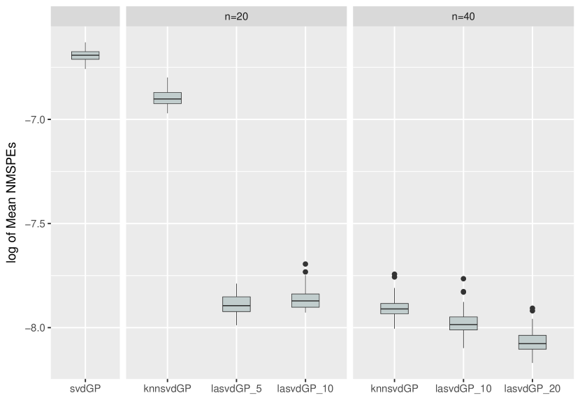
Figure 1: The boxplots of the log of mean NMSPE computed from 2,000 test points over 50 simulations for the computer simulator (15). The proposed lasvdGP approach achieves much smaller log of mean NMSPE values than the competitors.

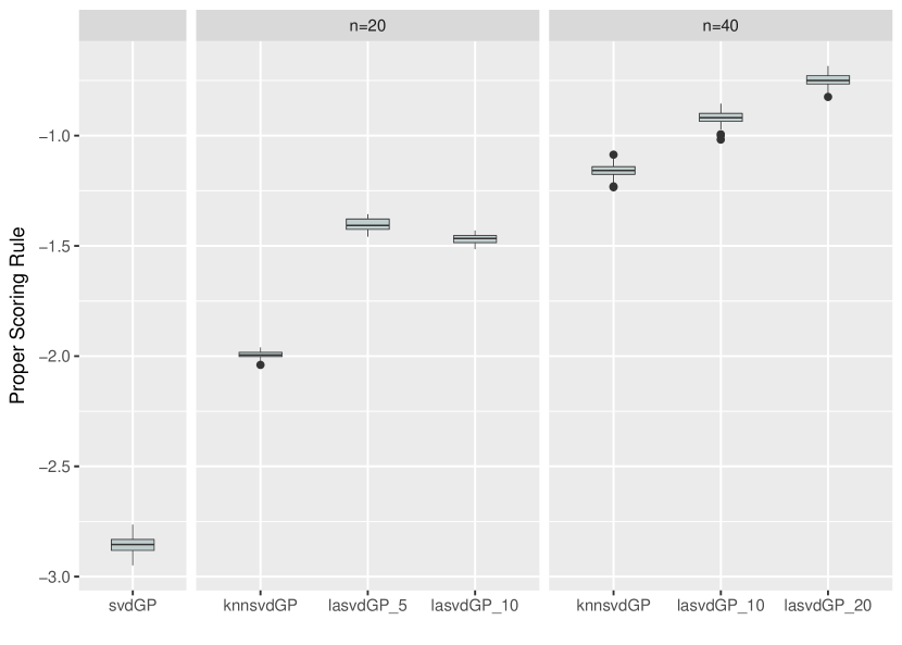
Figure 2: The boxplots of the mean proper scoring rule computed from 2,000 test points over 50 simulations for the computer simulator (15). The proposed lasvdGP approach achieves higher values of mean proper scoring rule than the competitors.

Figures 1 and 2 reveal that the proposed algorithm outperforms its naive counterpart irrespective of the total neighborhood size $(n)$. As the neighborhood size gets large, the prediction accuracy of the local approximation algorithms improves.

For a fixed data set of size 10,000, we also computed Monte Carlo cross-validation based values for the two measures, log of mean NMSPE and mean proper scoring rule, and compared the three models. We considered one-fifth of the data as the test set and the remaining as the training set. The boxplots of the two measures over 50 random splits of the data show the similar trend as in Figures 1 and 2.

4.2.   Example 2 (Bliznyuk et al. (2008))

Consider the environmental model in Bliznyuk et al. (2008) which models a pollutant spill caused by a chemical accident. The simulator output is given by

$$\begin{aligned} &f(\bm{x},t)=\frac{M}{\sqrt{Dt}}\exp\left(\frac{-s^{2}}{4Dt}\right)+\frac{M}{\sqrt{D(t-\tau)}}\exp\left(-\frac{(s-L)^{2}}{4D(t-\tau)}\right)I(\tau<t),\end{aligned}$$ (16)

where $\bm{x}=(M,D,L,\tau,s)^{T}$, $M$ denotes the mass of pollutant spilled at each location, $D$ is diffusion rate in the channel, $L$ is location of the second spill, $\tau$ is time of the second spill, $\bm{x}\in[7,13]\times[0.02,0.12]\times[0.01,3]\times[30.01,30.295]\times[0,3]$, and $t\in[0.3,60]$ is on a regular 200-point equidistant time grid.

In this example as well, we use the training data of size $N=10,000$ and the test data of size $M=2,000$ obtained using a random LHD. Similar to the previous example, Figures 3 and 4 display the boxplots of 50 log of mean NMSPEs and mean proper scoring rule values, respectively, computed over the test set.

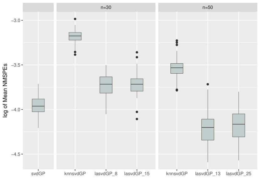
Figure 3: The boxplots of the log of mean NMSPEs computed from 2,000 test points over 50 simulations for the simulator given by (16). The proposed lasvdGP approach achieves much smaller log of mean NMSPE values than the competitors.

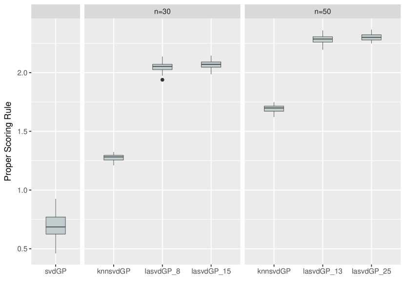
Figure 4: The boxplots of mean proper scoring rule computed from 2,000 test points over 50 simulations for the simulator given by (16). The proposed lasvdGP approach achieves higher values of mean proper scoring rule than the competitors.

Focussing on the local GP models, Figures 3 and 4 demonstrate that the proposed approach (lasvdGP) is more accurate than the naive one (knnsvdGP), and $n=50$ exhibits more accurate prediction than $n=30$. As in the previous example, the Monte Carlo cross-validation approach shows consistent findings. To investigate this further, we compared the prediction accuracy of lasvdGP for different $n$ and $n_{0}=\lceil n/2\rceil$, Figure 5 summarizes the findings.

Figure 5: The boxplots of the log of mean NMSPEs computed using 2,000 test points over 50 simulations with $n=30,50,100,200$ and $n_{0}=n/2$ for model (16). As the neighborhood size increases, the log of mean NMSPE values by the proposed lasvdGP approach decrease, resulting in more accurate prediction.

Figure 5 shows the expected increasing trend of the average prediction accuracy. Though the prediction accuracy increases with $n$, the rate of increment in the accuracy slows down as $n$ increases, and more importantly, note that fitting a lasvdGP model, requires $O(n^{3}NM)$ flops, which becomes prohibitively large very quickly.

4.3.   Example 3 (TDB simulator - Teismann et al. (2009))

The two-delay blowfly (TDB) model (Teismann et al. (2009)) simulates European red mites (ERM) population dynamics under predator-prey interactions in apple orchards via numerically solving the Nicholson’s blowfly differential equation (Gurney et al. (1980)). Unmanaged ERM population growth could incur massive infestation which inflicts heavy loss in apple industry. Therefore, the monitoring and subsequent intervention of ERM population dynamics is of vital importance for apple orchards management. The objective here is to emulate this simulator for deeper insight in the process.

The TDB model takes eleven input variables (e.g., death rates for different stages, fecundity, hatching time, survival rates, and so on) and returns the time series (at 28 time points) of ERM population evolutions at three stages, i.e., eggs, juveniles and adults (see Ranjan et al. (2016) for details). In this paper, we focus on the population dynamics of juveniles. Figure 6 shows the model output at five randomly chosen input points.

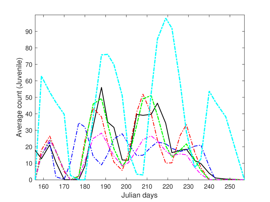
Figure 6: Juvenile ERM population dynamics as outputs of the TDB model at five different inputs. The solid curve shows the field data, and the dashed curves show the TDB outputs.

The input variable domains are decided by expert knowledge. For convenience, we transform the inputs into 11-dimensional unit hypercube. Given that we have a limited (data) budget from the simulator, we rely on the Monte Carlo cross-validation error alone. We had access to a data set of size 30,000 for the emulation and prediction accuracy measurements. For such a large scale dynamic computer model, svdGP is computationally infeasible. We used $n=80$ and $n_{0}=\lceil n/2\rceil$ for the proposed local SVD-based GP models. For each method, the total data was partitioned into training and test set in 4:1 ratio, and then the prediction accuracy measures were computed on the test set. Figure 7 shows the boxplots of the log of mean NMSPEs and mean proper scoring rule values over 50 randomly chosen Monte Carlo partitions.

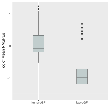
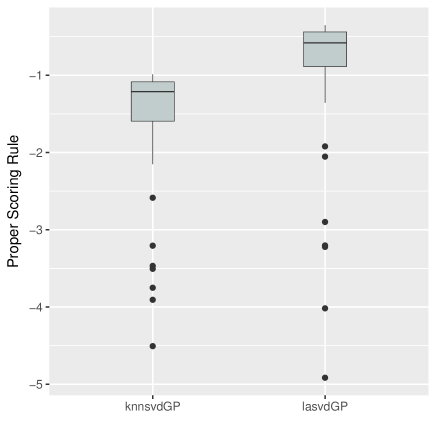
Figure 7: The boxplots of the log of mean NMSPEs (left) and mean proper scoring rule (right) for the TDB application obtained via Monte Carlo cross-validation. The proposed lasvdGP approach outperforms the knnsvdGP approach in terms of both log of mean NMSPEs and the mean proper scoring rule.

5.   Concluding Remarks

We have proposed local approximate SVD-based GP models for large-scale dynamic computer experiments. The proposed local SVD-based GP models with the proposed neighborhood selection algorithm reduce the time complexity of the full SVD-based GP models. Though slightly more time consuming than its naive counterpart, lasvdGP has been shown to be much more accurate in prediction for both simulation examples and the real data analysis. With the assistance of parallel computation, the proposed algorithm can easily handle dynamic computer experiments with training set as large as (approx) 25,000 points, which is beyond the capacity of the full model.

There are a few remarks worth mentioning. First, in this article, we refer to large-scale dynamic computer experiments as those with a large number of inputs. This is different from the large data aspect in Gu et al. (2016) where the spatial-temporal applications with small run sizes (in the order of hundreds) but large numbers of time points (in the order of tens of thousands) were considered. In their application, fitting full SVD-based GP models are still computationally feasible, as the number of significant singular values might be large but the number of inputs (for $n\times n$ correlation matrix factorization) would be small.

Second, the formula (10) does not consider the possible update of the estimated correlation parameters. If new data arrives, the empirical Bayesian estimators of correlation parameters $\bm{\theta}$’s in (8) are expected to change with the training set. To address this issue, Gramacy and Apley (2015) suggested the second order Taylor polynomial approximation.

Third, there are possible improvements in terms of computational efficiency. In searching for neighborhood set, it has been suggested to consider more sophisticate searches such as using graphical processing units (GPUs) and approximating discrete neighborhood searches via continuous ones along the rays emanating from each predictive point (Franey et al. (2012); Gramacy and Haaland (2016)). Another way to boost the computational efficiency is that instead of searching the neighborhood set for each individual point in the prediction set $\bm{X}^{*}$, some clustering algorithms could be performed on $\bm{X}^{*}$ to divide it into groups on which the proposed neighborhood selection is executed. These are interesting topics for our future research.

Supplementary Materials

The supplementary material includes the following:

Appendix:

Section A contains the proof of Proposition 1. Section B presents two algorithms (in the formal algorithm format) for fitting local approximate SVD-based GP models (lasvdGP) described in Sections 2 and 3 of this article. Section C summarizes simulation results for establishing the reliability of the estimated range parameters (or equivalently, the correlation parameters) for the proposed lasvdGP model fits in Examples 1 and 2. (Appendix.pdf, PDF file)

Code:

R codes to reproduce results in the article are available in the zip file. Details can be found in the readme.txt file included. (code.zip, zipped folder)

Supplementary Materials

A. Proof Of Proposition 1

Following (7), the inner expectation in (10) can be written as

$$\begin{aligned} &\text{E}\Big{[}\big{\|}\bm{y}(\bm{x}_{0})-\hat{\bm{y}}(\bm{x}_{0}|\bm{c}(\bm{x}),\bm{V}^{*(k)},\hat{\bm{\Theta}}^{(k)})\big{\|}^{2}\Big{|}\bm{c}(\bm{x}),\bm{V}^{*(k)},\hat{\bm{\Theta}}^{(k)},(\hat{\sigma}^{(k)})^{2}\Big{]}\\ =&\text{tr}\Big{(}\bm{B}^{(k)}\bm{\Lambda}\big{(}\bm{V}^{*(k)}(\bm{x}),\hat{\bm{\Theta}}^{(k)}\big{)}(\bm{B}^{(k)})^{T}+(\hat{\sigma}^{(k)})^{2}\bm{I}_{L}\Big{)}\\ =&(\hat{\sigma}^{(k)})^{2}L+\text{tr}\Big{(}\bm{\Lambda}\big{(}\bm{V}^{*(k)}(\bm{x}),\hat{\bm{\Theta}}^{(k)}\big{)}(\bm{B}^{(k)})^{T}\bm{B}^{(k)}\Big{)}\\ =&(\hat{\sigma}^{(k)})^{2}L+\sum_{i=1}^{p_{k}}(d_{i}^{(k)})^{2}\hat{\sigma}^{2}_{i}\big{(}\bm{x}_{0}|\bm{v}_{i}^{(k)}(\bm{x}),\hat{\bm{\theta}}_{i}^{(k)}\big{)},\end{aligned}$$ (A.17)

where $\bm{V}^{*(k)}(\bm{x})=[(\bm{V}^{*(k)})^{T},\bm{c}(\bm{x})]^{T}$ and $d^{(k)}_{i}$ is the $i$th largest singular value of $\bm{Y}^{(k)}$,

$$\bm{\Lambda}\big{(}\bm{V}^{*(k)}(\bm{x}),\hat{\bm{\Theta}}^{(k)}\big{)}=\text{diag}\Big{(}\hat{\sigma}^{2}_{1}\big{(}\bm{x}_{0}|\bm{v}_{1}^{(k)}(\bm{x}),\hat{\bm{\theta}}^{(k)}_{1}\big{)},\dots,\hat{\sigma}^{2}_{p_{k}}\big{(}\bm{x}_{0}|\bm{v}_{p_{k}}^{(k)}(\bm{x}),\hat{\bm{\theta}}^{(k)}_{p_{k}}\big{)}\Big{)},$$

and

$$\hat{\sigma}^{2}_{i}\big{(}\bm{x}_{0}|\bm{v}_{i}^{(k)}(\bm{x}),\hat{\bm{\theta}}^{(k)}_{i}\big{)}=\frac{\rho^{(k)}_{i}(\bm{x}_{0},\bm{x})}{\alpha_{i}+k}\big{(}\beta_{i}+\psi_{i}^{(k)}(\bm{x})\big{)},$$

for $i=1,\dots,p_{k}$, where $\psi_{i}^{(k)}(\bm{x})=\bm{v}_{i}^{(k)}(\bm{x})^{T}\tilde{\bm{K}}_{i}^{-1}(\bm{x})\bm{v}_{i}^{(k)}(\bm{x})$, and $\bm{v}_{i}^{(k)}(\bm{x})=[(\bm{v}_{i}^{(k)})^{T},c_{i}(\bm{x})]^{T}$ is the $i$th column of $\bm{V}^{*(k)}(\bm{x})$.

The first equality of (A.17) follows from Theorem 3.2b.1 of Mathai and Provost (1992). The third equality is derived from the column-orthogonality of $\bm{B}^{(k)}$, i.e. $(\bm{B}^{(k)})^{T}\bm{B}^{(k)}=(\bm{D}^{*(k)})^{2}$. Plugging (A.17) into (10), we get

$$J(\bm{x}_{0},\bm{x}) =\text{E}\Big{[}(\hat{\sigma}^{(k)})^{2}L+\sum_{i=1}^{p_{k}}(d_{i}^{(k)})^{2}\hat{\sigma}^{2}_{i}\big{(}\bm{x}_{0}|\bm{v}_{i}^{(k)}(\bm{x}),\hat{\bm{\theta}}_{i}^{(k)}\big{)}\Big{|}\bm{V}^{*(k)},\hat{\bm{\Theta}}^{(k)},(\hat{\sigma}^{(k)})^{2}\Big{]}$$

$$=(\hat{\sigma}^{(k)})^{2}L+\sum_{i=1}^{p_{k}}(d_{i}^{(k)})^{2}\Big{(}\frac{\rho_{i}^{(k)}(\bm{x}_{0},\bm{x})}{\alpha_{i}+k}\big{(}\beta_{i}+\text{E}[\psi_{i}^{(k)}(\bm{x})|\bm{V}^{*(k)},\hat{\bm{\Theta}}^{(k)},(\hat{\sigma}^{(k)})^{2}]\big{)}\Big{)}$$

$$=(\hat{\sigma}^{(k)})^{2}L+\sum_{i=1}^{p_{k}}(d_{i}^{(k)})^{2}\Big{(}\frac{\rho_{i}^{(k)}(\bm{x}_{0},\bm{x})}{\alpha_{i}+k}\big{(}\beta_{i}+\text{E}[\psi_{i}^{(k)}(\bm{x})|\bm{v}^{(k)}_{i},\hat{\bm{\theta}}^{(k)}_{i}]\big{)}\Big{)}$$

$$=(\hat{\sigma}^{(k)})^{2}L+\sum_{i=1}^{p_{k}}(d_{i}^{(k)})^{2}\Big{(}\frac{\rho_{i}^{(k)}(\bm{x}_{0},\bm{x})}{\alpha_{i}+k}\big{(}\beta_{i}+\frac{\alpha_{i}+k}{\alpha_{i}+k-1}\psi_{i}^{(k)}\big{)}\Big{)}.$$

The second equality holds because $\rho^{(k)}_{i}(\bm{x}_{0},\bm{x})$ is a deterministic function of $\bm{x}_{0}$, $\bm{x}$ and $\hat{\bm{\theta}}_{i}^{(k)}$. The third equality follows from the independence among $c_{i}$’s. The validity of the fourth equality is due to Gramacy and Apley (2015).

B. Algorithms

Algorithm 1 summarizes the key steps required for estimating the necessary parameters in the posterior predictive distribution (Equation (9) of the main article) of a full SVD-based GP model fitted to a training data of size $N$.

Input : (1) Training set: $\bm{X}_{N\times q}$, (2) response matrix: $\bm{Y}_{L\times N}$, (3) threshold $\gamma$,

(4) prior parameters: $\bm{\alpha}=[\alpha_{1},\dots,\alpha_{p},\alpha]^{T}$, $\bm{\beta}=[\beta_{1},\dots,\beta_{p},\beta]^{T}$.

Output : (1) Basis $\bm{B}_{N\times p}$, (2) singular values $\bm{D}^{*}_{p\times p}$, (3) coefficients $\bm{V}^{*}$,

(4) correlation parameters $\hat{\bm{\Theta}}$, (5) variance $\hat{\sigma}^{2}$.

1 Function svdGP($\bm{X}$,$\bm{Y}$,$\bm{\alpha}$,$\bm{\beta}$,$\gamma$)

2      

3      $[\bm{B},\bm{D}^{*},\bm{V}^{*},p]\leftarrow$ buildBasis($\bm{Y}$,$\gamma$)

4       $\bm{r}\leftarrow\text{vec}(\bm{Y})-(\bm{I}_{N}\otimes\bm{B})\text{vec}(\bm{V}^{*T})$

5       $\hat{\sigma}_{i}^{2}(\bm{x}_{0}|\bm{v}_{i},\bm{\theta}_{i})=(\beta_{i}+\psi_{i})\Big{(}1-\bm{k}^{T}_{i}(\bm{x}_{0})\bm{K}^{-1}_{i}\bm{k}_{i}(\bm{x}_{0})\Big{)}/(\alpha_{i}+N)$, $\hat{\sigma}^{2}\leftarrow\big{(}\bm{r}^{T}\bm{r}+\beta\big{)}/(NL+\alpha+2)$

6       $\hat{\bm{\Theta}}\leftarrow$ inference($\bm{V}^{*}$, $p$, $\bm{\alpha}$, $\bm{\beta}$)

7       return $\bm{B}$, $\bm{D}^{*}$, $\bm{V}^{*}$, $\hat{\bm{\Theta}}$, $\hat{\sigma}^{2}$

8 Subroutine buildBasis($\bm{Y}$,$\gamma$)

       $[\bm{U},\bm{D},\bm{V}]\leftarrow$SVD($\bm{Y}$)

        /* perform SVD on matrix $\bm{Y}$. */

       $p\leftarrow\min\left\{m:\frac{\sum_{i=1}^{m}d_{i}}{\sum_{i=1}^{k}d_{i}}>\gamma\right\}$

        /* where $\bm{D}=\text{diag}(d_{1},\dots,d_{N}),k=\min\{N,L\}$ */

       $\bm{B}\leftarrow\bm{U}^{*}\bm{D}^{*}$

        /* as in Section 2.1 */

9       return $\bm{B}$, $\bm{D}^{*}$, $\bm{V}^{*}$, $p$

10 Subroutine inference($\bm{V}^{*}$, $p$, $\bm{\alpha}$, $\bm{\beta}$)

11       for $i\leftarrow 1$ to $p$ do

             $\hat{\bm{\theta}}_{i}\leftarrow\underset{\bm{\theta}_{i}}{\mathrm{argmax}}\>\pi(\bm{\theta}_{i}|\bm{v}_{i})$

              /* fit $p$ independent GPs by finding the MAPs */

12            

13      return $\hat{\bm{\Theta}}=[\hat{\bm{\theta}}_{1},\dots,\hat{\bm{\theta}}_{p}]^{T}$

Algorithm 1 SVD-based GP model

Algorithm 2 presents the steps required for fitting the proposed local approximate SVD-based GP model (lasvdGP) with the neighbourhood points selected using the $J$-criterion in Section 3.1 of the main article.

Input : (1) Training set: $\bm{X}_{N\times q}$, (2) response matrix: $\bm{Y}_{L\times N}$, (3) test set $\bm{X}^{*}_{M\times q}$,

(4) neighborhood size $n$, (5) initial neighborhood size $n_{0}$, (6) threshold $\gamma$,

(7) prior parameters $\bm{\alpha}=[\alpha_{1},\dots,\alpha_{p},\alpha]^{T}$ and $\bm{\beta}=[\beta_{1},\dots,\beta_{p},\beta]^{T}$.

Output : (1) The predicted mean response, and (2) the associated posterior variance in estimating $\bm{y}(\bm{x}_{0})$ for each $\bm{x}_{0}\in\bm{X}^{*}$.

1 for each $\bm{x}_{0}\in\bm{X}^{*}$ do

       $\bm{X}^{(n_{0})}\leftarrow\{\bm{x}_{i},i=1,\dots,n_{0}\}$

        /* $n_{0}$ nearest neighbours of $\bm{x}_{0}$ in $\bm{X}$ as in knn */

2       $\bm{Y}^{(n_{0})}\leftarrow\{y(\bm{x}):\bm{x}\in\bm{X}^{(n_{0})}\}$

3       for $k\leftarrow n_{0}$ to $n-1$ do

4             $[\bm{B}^{(k)},\bm{D}^{*(k)},\bm{V}^{*(k)},p_{k},\hat{\bm{\Theta}}^{k},(\hat{\sigma}^{(k)})^{2},(\hat{\bm{\sigma}}^{(k)})^{2}]\leftarrow$svdGP($\bm{X}^{(k)}$,$\bm{Y}^{(k)}$,$\bm{\alpha}$,$\bm{\beta}$,$\gamma$)

5             $\bm{x}^{*}_{k+1}\leftarrow\underset{\bm{x}\in\bm{X}\backslash\bm{X}^{(k)}}{\mathrm{argmin}}\>J(\bm{x}_{0},\bm{x})$

6             $\bm{X}^{(k+1)}\leftarrow\bm{X}^{(k)}\cup\bm{x}_{k+1}^{*}$

7             $\bm{Y}^{(k+1)}\leftarrow\bm{Y}^{(k)}\cup\bm{y}(\bm{x}^{*}_{k+1})$

8            

9      $[\bm{B}^{(n)},\bm{D}^{*(n)},\bm{V}^{*(n)},p_{n},\hat{\bm{\Theta}}^{(n)},(\hat{\sigma}^{(n)})^{2},(\hat{\bm{\sigma}}^{(n)})^{2}]\leftarrow$ svdGP($\bm{X}^{(n)}$,$\bm{Y}^{(n)}$,$\bm{\alpha}$,$\bm{\beta}$,$\gamma$)

10       Predict $\bm{y}(\bm{x}_{0})$ through $\pi(\bm{y}(\bm{x}_{0})|\bm{V}^{*(n)},\hat{\bm{\Theta}}^{(n)},(\hat{\sigma}^{(n)})^{2},(\hat{\bm{\sigma}}^{(n)})^{2})$ in Eqn. (9)

11      

Algorithm 2 Proposed local SVD-based GP model

C. Additional Simulation Results

We now investigate the reliability of the estimated range parameters (or equivalently, the correlation parameters) for the proposed local approximate SVD-based GP model (lasvdGP) fits in Examples 1 (Forrester et al., 2008 – $q=3,N=10000,M=2000$, $n=40$ and $n_{0}=20$) and 2 (Bliznyuk et al., 2008 – $q=5,N=10000,M=2000$, $n=50$ and $n_{0}=25$) of the main article.

To explain the results, recall that for each point in the test set, the SVD-based GP model fitted on the neighbourhood set is represented using a $p$-dimensional basis as in Equation (1), where $p$ is selected by the cumulative percentage criterion (Equation (2)). That is, for each test point, $p$ independent GP models for each $c_{i}(\textbf{x})$ are fitted in the respective neighbourhood searched. The value of $p$ may be different for different test points. The frequency table of the number of leading basis functions for 2,000 test points for each of the two examples are displayed in Table 2.

	$p$
	3	4	5	6	7	8	total
Example 1	266	1734	0	0	0	0	2000
Example 2	15	161	873	825	124	2	2000

Table 2: Frequency of $p$ among the 2,000 test points in Examples 1 and 2.

For simplicity, we only report the estimated range parameters in the GP models corresponding to $c_{1}(\bm{x})$, $c_{2}(\bm{x})$ and $c_{3}(\bm{x})$ from the final fits, i.e., after $n-n_{0}$ follow-up points were added. Figures 8 and 9 display the boxplots of those 2,000 estimates for each range parameter in Examples 1 and 2, respectively.

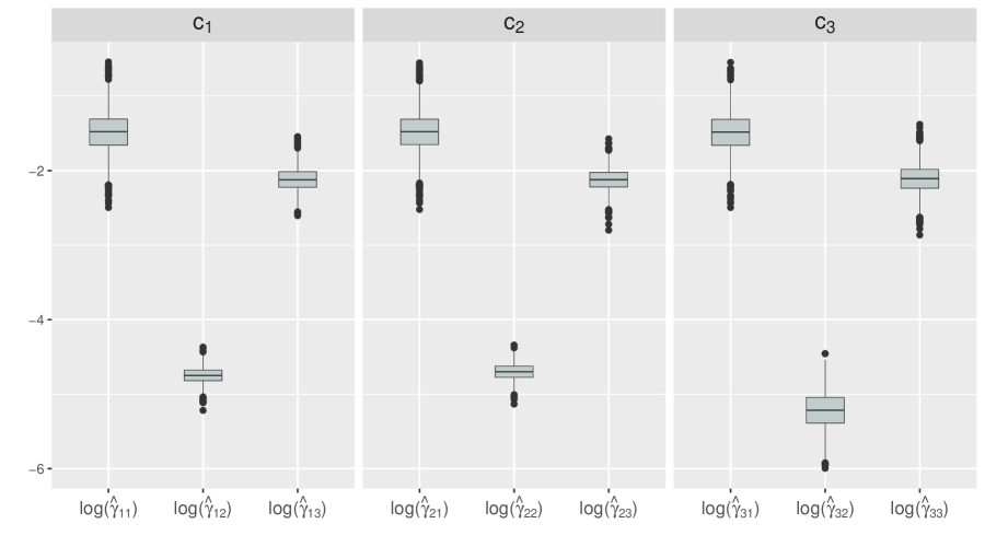
Figure 8: The boxplots of the 2,000 estimates of the log-range parameters in the GP models for $c_{1}(\bm{x})$, $c_{2}(\bm{x})$ and $c_{3}(\bm{x})$ in Example 1 (Forrester et al., 2008).

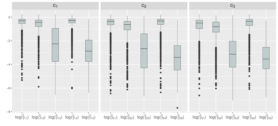
Figure 9: The boxplots of the 2,000 estimates of the log-range parameters in the GP models for $c_{1}(\bm{x})$, $c_{2}(\bm{x})$ and $c_{3}(\bm{x})$ in Example 2 (Bliznyuk et al., 2008).

REFERENCES

- Bayarri et al. (2007) Bayarri, M., J. Berger, J. Cafeo, G. Garcia-Donato, F. Liu, J. Palomo, R. Parthasarathy, R. Paulo, J. Sacks, and D. Walsh (2007). Computer model validation with functional output. The Annals of Statistics 35(5), 1874–1906.
- Bingham et al. (2014) Bingham, D., P. Ranjan, and W. J. Welch (2014). Statistics in action: A canadian outlook. Sequential design of computer experiments for optimization, estimating contours, and related objectives, 109–124.
- Bliznyuk et al. (2008) Bliznyuk, N., D. Ruppert, C. Shoemaker, R. Regis, S. Wild, and P. Mugunthan (2008). Bayesian calibration and uncertainty analysis for computationally expensive models using optimization and radial basis function approximation. Journal of Computational and Graphical Statistics 17(2), 270–294.
- Cohn (1996) Cohn, D. A. (1996). Neural network exploration using optimal experiment design. Neural networks 9(6), 1071–1083.
- Cohn et al. (1996) Cohn, D. A., Z. Ghahramani, and M. I. Jordan (1996). Active learning with statistical models. Journal of Artificial Intelligence Research 4, 129–145.
- Conti et al. (2009) Conti, S., J. P. Gosling, J. E. Oakley, and A. O’Hagan (2009). Gaussian process emulation of dynamic computer codes. Biometrika 96(3), 663–676.
- Conti and O’Hagan (2010) Conti, S. and A. O’Hagan (2010). Bayesian emulation of complex multi-output and dynamic computer models. Journal of statistical planning and inference 140(3), 640–651.
- Emery (2009) Emery, X. (2009). The kriging update equations and their application to the selection of neighboring data. Computational Geosciences 13(3), 269–280.
- Farah et al. (2014) Farah, M., P. Birrell, S. Conti, and D. D. Angelis (2014). Bayesian emulation and calibration of a dynamic epidemic model for A/H1N1 influenza. Journal of the American Statistical Association 109(508), 1398–1411.
- Forrester et al. (2008) Forrester, A., A. Sobester, and A. Keane (2008). Engineering design via surrogate modelling: a practical guide. John Wiley & Sons.
- Franey et al. (2012) Franey, M., P. Ranjan, and H. Chipman (2012). A short note on Gaussian process modeling for large datasets using graphics processing units. arXiv:1203.1269.
- Gelman et al. (2014) Gelman, A., J. B. Carlin, H. S. Stern, and D. B. Rubin (2014). Bayesian data analysis, Volume 2. Chapman & Hall/CRC Boca Raton, FL, USA.
- Gentle (2007) Gentle, J. E. (2007). Matrix algebra: theory, computations, and applications in statistics. Springer Science & Business Media: New York.
- Gneiting and Raftery (2007) Gneiting, T. and A. E. Raftery (2007). Strictly proper scoring rules, prediction, and estimation. Journal of the American Statistical Association 102(477), 359–378.
- Gramacy (2005) Gramacy, R. B. (2005). Bayesian treed Gaussian process models. Ph. D. thesis, University of California Santa Cruz.
- Gramacy (2016) Gramacy, R. B. (2016). laGP: Large-scale spatial modeling via local approximate Gaussian processes in R. Journal of Statistical Software 72(1), 1–46.
- Gramacy and Apley (2015) Gramacy, R. B. and D. W. Apley (2015). Local Gaussian process approximation for large computer experiments. Journal of Computational and Graphical Statistics 24(2), 561–578.
- Gramacy and Haaland (2016) Gramacy, R. B. and B. Haaland (2016). Speeding up neighborhood search in local Gaussian process prediction. Technometrics 58(3), 294–303.
- Gramacy and Lee (2012) Gramacy, R. B. and H. K. Lee (2012). Cases for the nugget in modeling computer experiments. Statistics and Computing 22(3), 713–722.
- Gu et al. (2016) Gu, M., J. O. Berger, et al. (2016). Parallel partial Gaussian process emulation for computer models with massive output. The Annals of Applied Statistics 10(3), 1317–1347.
- Gu et al. (2017) Gu, M., X. Wang, and J. O. Berger (2017). Robust Gaussian stochastic process emulation. arXiv:1708.04738.
- Gurney et al. (1980) Gurney, W., S. Blythe, and R. Nisbet (1980). Nicholson’s blowflies revisited. Nature 287, 17–21.
- Hager (1989) Hager, W. W. (1989). Updating the inverse of a matrix. SIAM review 31(2), 221–239.
- Higdon et al. (2008) Higdon, D., J. Gattiker, B. Williams, and M. Rightley (2008). Computer model calibration using high-dimensional output. Journal of the American Statistical Association 103(482), 570–583.
- Hung et al. (2015) Hung, Y., V. R. Joseph, and S. N. Melkote (2015). Analysis of computer experiments with functional response. Technometrics 57(1), 35–44.
- Jones et al. (1998) Jones, D. R., M. Schonlau, and W. J. Welch (1998). Efficient global optimization of expensive black-box functions. Journal of Global Optimization 13(4), 455–492.
- Kennedy and O’Hagan (2001) Kennedy, M. C. and A. O’Hagan (2001). Bayesian calibration of computer models. Journal of the Royal Statistical Society: Series B 63(3), 425–464.
- Liu and West (2009) Liu, F. and M. West (2009). A dynamic modelling strategy for Bayesian computer model emulation. Bayesian Analysis 4(2), 393–411.
- McKay et al. (1979) McKay, M. D., R. J. Beckman, and W. J. Conover (1979). A comparison of three methods for selecting values of input variables in the analysis of output from a computer code. Technometrics 42(1), 55–61.
- Peng and Wu (2014) Peng, C.-Y. and C. J. Wu (2014). On the choice of nugget in kriging modeling for deterministic computer experiments. Journal of Computational and Graphical Statistics 23(1), 151–168.
- R Core Team (2017) R Core Team (2017). R: A Language and Environment for Statistical Computing. Vienna, Austria: R Foundation for Statistical Computing.
- Ranjan et al. (2008) Ranjan, P., D. Bingham, and G. Michailidis (2008). Sequential experiment design for contour estimation from complex computer codes. Technometrics 50(4), 527–541.
- Ranjan et al. (2011) Ranjan, P., R. Haynes, and R. Karsten (2011). A computationally stable approach to Gaussian process interpolation of deterministic computer simulation data. Technometrics 53(4), 366–378.
- Ranjan et al. (2016) Ranjan, P., M. Thomas, H. Teismann, and S. Mukhoti (2016). Inverse problem for a time-series valued computer simulator via scalarization. Open Journal of Statistics 6(03), 528–544.
- Rasmussen and Williams (2006) Rasmussen, C. E. and C. K. I. Williams (2006). Gaussian processes for machine learning. The MIT Press.
- Sacks et al. (1989) Sacks, J., W. J. Welch, T. J. Mitchell, and H. P. Wynn (1989). Design and analysis of computer experiments. Statistical Science 4(4), 409–423.
- Santner et al. (2003) Santner, T. J., B. J. Williams, and W. I. Notz (2003). The design and analysis of computer experiments. Springer Science & Business Media: New York.
- Shao (1993) Shao, J. (1993). Linear model selection by cross-validation. Journal of the American statistical Association 88(422), 486–494.
- Stein (2005) Stein, M. L. (2005). Space–time covariance functions. Journal of the American Statistical Association 100(469), 310–321.
- Teismann et al. (2009) Teismann, H., R. Karsten, R. Hammond, J. Hardman, and J. Franklin (2009). On the possibility of counter-productive intervention: the population mean for blowflies models can be an increasing function of the death rate. Journal of Biological Systems 17(04), 739–757.