Critical quench dynamics of random quantum spin chains: Ultra-slow relaxation from initial order and delayed ordering from initial disorder

Abstract

By means of free fermionic techniques combined with multiple precision arithmetic we study the time evolution of the average magnetization, $\overline{m}(t)$, of the random transverse-field Ising chain after global quenches. We observe different relaxation behaviors for quenches starting from different initial states to the critical point. Starting from a fully ordered initial state, the relaxation is logarithmically slow described by $\overline{m}(t)\sim\ln^{a}t$, and in a finite sample of length $L$ the average magnetization saturates at a size-dependent plateau $\overline{m}_{p}(L)\sim L^{-b}$; here the two exponents satisfy the relation $b/a=\psi=1/2$. Starting from a fully disordered initial state, the magnetization stays at zero for a period of time until $t=t_{d}$ with $\ln t_{d}\sim L^{\psi}$ and then starts to increase until it saturates to an asymptotic value $\overline{m}_{p}(L)\sim L^{-b^{\prime}}$, with $b^{\prime}\approx 1.5$. For both quenching protocols, finite-size scaling is satisfied in terms of the scaled variable $\ln t/L^{\psi}$. Furthermore, the distribution of long-time limiting values of the magnetization shows that the typical and the average values scale differently and the average is governed by rare events. The non-equilibrium dynamical behavior of the magnetization is explained through semi-classical theory.

1 Introduction

Following the experimental progress in non-equilibrium dynamics of ultracold-atomic gases in optical lattices [1, 2, 3, 4, 5, 6, 7, 8, 9, 10, 11], there are tremendous theoretical efforts aimed at understanding the time-evolution of certain observables in closed quantum systems after a sudden or smooth change of Hamiltonian parameters. In a quench process both the functional form of the relaxation and the properties of the long-time, presumably stationary state are of interest [12, 13, 14, 15, 16, 17, 18, 19, 20, 21, 22, 23, 24, 25, 26, 27, 28, 29, 30, 31, 32, 33, 34, 35, 36, 37, 38, 39, 40, 41, 42, 43, 44, 45, 46, 47, 48, 49, 50, 51, 52, 53, 54, 55, 56, 57, 58, 59, 60, 61, 62, 63, 64, 65, 66, 67, 68, 69]. In homogeneous systems the order parameter has an exponential relaxation, while the entanglement entropy between a subsystem and its environment grows linearly in time after a quench. These phenomena have been explained in the frame of a semi-classical theory. According to the theory, during the quench process quasi-particles are created uniformly in the sample and move ballistically [36, 18, 41, 42]. Concerning the long-time limit of the relaxation process integrable and non-integrable systems show different behaviors. Non-integrable systems are expected to thermalize [16, 17, 18, 19, 20, 21, 22, 23, 24, 25, 26], but there are some counterexamples [62, 63, 64]. On the other hand, integrable systems in the stationary state are generally described by a so-called generalized Gibbs ensemble, which includes all the conserved quantities of the system. Recently it has been observed that in certain models both local and quasi-local conserved quantities have to be taken into account to construct an appropriate generalized Gibbs ensemble [57, 58, 59, 60, 61, 65, 66, 67, 68, 69].

In a system with spatial inhomogeneities, such as defects [70, 71, 72, 73, 74, 75, 76], quasi-periodic or aperiodic interactions [77, 78, 79], the non-equilibrium relaxation process becomes qualitatively different from the homogeneous case. In the semi-classical picture the quasi-particles are also inhomogeneously created and they move in a complex diffusive way. With randomness the eigenstates of the Hamiltonian can be localized, which leads to Anderson localization [80] in non-interacting systems or many-body localization [81] if the particles are interacting; in these cases the quasi-particles generally move only finite distances away from their place of creation or follow some ultra-slow diffusive motion. As a result the non-equilibrium long-time stationary state of disordered systems retains memory of the initial state and therefore thermalization does not take place [82].

Concerning the functional form of the relaxation process after a quench in random quantum systems, there have been detailed studies about the time-dependence of the entanglement entropy [83, 84, 85, 86, 87]. If the system consists of non-interacting fermions - such as the critical XX-spin chain with bond disorder or the critical random transverse-field Ising chain - the dynamical entanglement entropy grows ultraslowly in time as

$${\cal S}(t)\sim a\ln\ln t\,,$$ (1)

and saturates in a finite system at a value

$${\cal S}(\ell)\sim b\ln\ell\,,$$ (2)

where $\ell$ denotes the size of a block in a bipartite system and can be chosen to be proportional to the size of the system $L$ [84, 87]. These scaling forms can be explained by a strong disorder renormalization-group (SDRG) approach [88]. Recently, the SDRG method, which was designed as a ground state approach, has been generalized to take into account excited states [89, 90, 91]; this generalized RG method is often abbreviated as RSRG-X [89]. By this generalized SDRG method the ratio of the prefactors in (1) and (2) is predicted as $b/a=\psi_{\mathrm{ne}}$, where $\psi_{\mathrm{ne}}=1/2$ is a critical exponent in the non-equilibrium process and describes the relation between time-scale and length-scale as

$$\ln t\sim L^{\psi_{\mathrm{ne}}}\;.$$ (3)

For interacting fermion models due to many-body localization the time-dependence of the dynamical entropy is ${\cal S}(t)\sim\ln^{\omega}t$ with $\omega\geq 1$, while the saturation value follows the volume law, ${\cal S}(\ell)\sim\ell$ [86].

In the present paper we study the relaxation of the order parameter of the random transverse-field Ising chain after a quench to the critical final state and into a ferromagnetic state. We consider relaxation processes from an initial ferromagnetic state and from a fully paramagnetic state by a sudden change of the strength of the transverse field. To circumvent numerical instability as observed in previous calculations for large systems using eigenvalue solver routines [84, 87], we use multiple precision arithmetic to study the time-evolution through direct matrix multiplications.

The rest of the paper is organized as follows. The model and the method for calculating the local magnetization are described in section 2 . The numerical results for relaxation of the magnetization following different quench protocols are presented and discussed in section 3. A summary is given in section 4. Details of the time evolution of Majorana fermion operators are given in the appendix.

2 The model and the method

The model we consider is the random transverse-field Ising chain of length $L$ defined by the Hamiltonian:

$${\cal H}=-\frac{1}{2}\sum_{i=1}^{L-1}{J}_{i}\sigma_{i}^{x}{\sigma}_{i+1}^{x}-\frac{1}{2}\sum_{i=1}^{L}{h}_{i}{\sigma}_{i}^{z}\;,$$ (4)

in terms of the Pauli matrices ${\sigma}_{i}^{x,z}$ at site $i$. In this paper we will consider open chains with free boundary conditions. The couplings, ${J}_{i}$, and the transverse fields, ${h}_{i}$, are position dependent random numbers taken from the uniform distributions in the intervals $[0,1]$ and $[0,1]h$, respectively. The strength of the random transverse field, $h$, is time-dependent; for $t<0$ its value is $h_{0}$ and for $t>0$ it changes suddenly to $h\,(\neq h_{0})$. The initial and the final Hamiltonians are denoted by ${\cal H}_{0}$ and ${\cal H}$, respectively. The system for $t<0$ is prepared in the ground state $|\Psi_{0}^{(0)}\rangle$ of the initial Hamiltonian; after the quench for $t>0$ the system evolves according to the final Hamiltonian ${\cal H}$ and the state of the system is described by $|\Psi_{0}(t)\rangle=\exp(-\imath{\cal H}t)|\Psi_{0}^{(0)}\rangle$, which is generally not an eigenstate of ${\cal H}$. Here and throughout the paper we denote the imaginary unit $\sqrt{-1}$ by $\imath$ to avoid confusion with the integer index $i$ and set $\hbar=1$. To calculate the time-dependent expectation value $A(t)$ of an observable $\hat{A}$, we work in the Heisenberg picture using $\hat{A}_{H}(t)=\exp(\imath{\cal H}t)\hat{A}\exp(-\imath{\cal H}t)$ and evaluate $A(t)=\langle\Psi_{0}^{(0)}|\hat{A}_{H}(t)|\Psi_{0}^{(0)}\rangle$. Time-dependent matrix elements and correlation functions are calculated in a similar way.

The standard way to deal with the Hamiltonian of the transverse field Ising chain is the mapping to spinless free fermions [92, 93]. The spin operators ${\sigma}_{i}^{x,y,z}$ are expressed in terms of fermion creation (annihilation) operators ${c}_{i}^{\dagger}$ (${c}_{i}$) by using the Jordan-Wigner transformation [94]: ${c}^{\dagger}_{i}={a}_{i}^{+}\exp\left[\pi\imath\sum_{j}^{i-1}{a}_{j}^{+}{a}_{j}^{-}\right]$ and ${c}_{i}=\exp\left[\pi\imath\sum_{j}^{i-1}{a}_{j}^{+}{a}_{j}^{-}\right]{a}_{i}^{-}$, where ${a}_{j}^{\pm}=({\sigma}_{j}^{x}\pm\imath{\sigma}_{j}^{y})/2$. The Ising Hamiltonian in (4) can then be written in a quadratic form in fermion operators:

$${\cal H}=-\sum_{i=1}^{L}h_{i}\left({c}^{\dagger}_{i}{c}_{i}-\frac{1}{2}\right)-\frac{1}{2}\sum_{i=1}^{L-1}J_{i}({c}^{\dagger}_{i}-{c}_{i})({c}^{\dagger}_{i+1}+{c}_{i+1})\;.$$

In this paper we are interested in the relaxation of the local order parameter (magnetization), $m_{l}(t)$, at a position $l$. Following the method by Yang [95], for a given sample of large length $L$ we define $m_{l}(t)$ as the off-diagonal matrix element of the longitudinal magnetization operator: $m_{l}(t)=\langle\Psi_{0}^{(0)}|{\sigma}_{l}^{x}(t)|\Psi_{1}^{(0)}\rangle$, where $|\Psi_{1}^{(0)}\rangle$ is the first excited state of ${\cal H}_{0}$. In the free-fermion representation we introduce two Majorana fermion operators, $\check{{a}}_{2i-1}$ and $\check{{a}}_{2i}$ at site $i$ with the definition:

$$\check{{a}}_{2i-1}={c}^{{\dagger}}_{i}+{c}_{i}$$

$$\check{{a}}_{2i}=-\imath({c}^{{\dagger}}_{i}-{c}_{i})\,,$$ (5)

which obey the commutation relations:

$$\check{{a}}_{i}^{+}=\check{{a}}_{i},\quad\{\check{{a}}_{i},\check{{a}}_{j}\}=2\delta_{i,j}\;.$$ (6)

The spin operators are then expressed in terms of the Majorana operators as:

$${\sigma}_{l}^{x} = \;\imath^{l-1}\prod_{j=1}^{2l-1}\check{{a}}_{j}\;.$$ (7)

The calculation of the magnetization, $m_{l}(t)$, involves the evaluation of the determinant of a $2l\times 2l$ antisymmetric matrix ${\bf C}$ with the elements being the correlation functions $C_{ij}=\langle\mathit{\Psi}^{(0)}_{0}|\check{{a}}_{i}(t)\check{{a}}_{j}(t)|\mathit{\Psi}^{(0)}_{0}\rangle$, for $i<j<2l$, $C_{i,2l}=\langle\mathit{\Psi}^{(0)}_{0}|\check{{a}}_{i}(t)|\mathit{\Psi}^{(0)}_{1}\rangle$, and $C_{ji}=-C_{ij}$. For details see the appendix of Ref. [78].

For a random system any physical quantity requires an averaging over disorder realizations. We denote the disorder average by an overbar; accordingly, the average local magnetization is expressed as

$$\overline{m}_{l}(t)=\overline{\langle\Psi_{0}^{(0)}|{\sigma}_{l}^{x}(t)|\Psi_{1}^{(0)}\rangle}\,.$$ (8)

2.1 In equilibrium

In equilibrium (i.e. for $t<0$), the critical behavior of the local magnetization $m_{l}(0)$ has been analytically studied by the SDRG method [96], and the random quantum critical point (at $h_{0}=h_{c}=1$) is found to be controlled by an infinite-randomness fixed point [97, 88]. In the thermodynamic limit ($L\to\infty$) one needs to discriminate between bulk ($l/L={\cal O}(1)$) and surface ($l={\cal O}(1)$) points, and the corresponding average magnetization is denoted by $\overline{m}$ and $\overline{m^{s}}$, respectively. In the ordered phase, $h_{0}<h_{c}=1$, we have $\overline{m}>0$, which vanishes at the critical point as $\overline{m}\sim(h_{c}-h_{0})^{\beta}$ with $\beta=(3-\sqrt{5})/2$. The surface magnetization follows similar behavior, however with a surface exponent $\beta_{s}=1$. At the critical point of a finite system the scaling of the average magnetization is governed by rare samples (or rare regions), which have the magnetization of order of ${\cal O}(1)$, whereas in typical samples the magnetization behaves as $m_{\mathrm{typ}}\sim\exp(-A\sqrt{L})$. The fraction of rare events scales as $P_{\mathrm{rare}}\sim L^{-x}$, and the same holds for the average magnetization: $\overline{m}\sim L^{-x}$; here the exponent $x=\beta/\nu$ is related to the critical exponent $\nu=2$ of the average correlation function. Similarly, the scaling behavior of the surface magnetization involves the exponent $x_{s}=\beta_{s}/\nu$. Concerning equilibrium dynamical scaling at the infinite-randomness fixed point, it is extremely space-time anisotropic so that the typical length, $\xi$, and the typical time, $\tau$, is related as

$$\ln\tau\sim\xi^{\psi}\;,$$ (9)

with an exponent $\psi=1/2$.

2.2 Out-of-equilibrium

Some out-of-equilibrium properties of the random transverse-field Ising chain have been predicted by the RSRG-X approach [89, 90, 91]. For a quench to the critical state, i.e. $h=h_{c}$ in the final Hamiltonian, the relation between the typical length scale and the typical time scale is in the same form as (9) in the equilibrium case and even the corresponding exponents are the same $\psi=\psi_{\mathrm{ne}}=1/2$ (cf. (3) and (9)). However, available numerical results [84, 87] for the relaxation of the entanglement entropy are not in complete agreement with the RSRG-X prediction.

Here we focus on the relaxation of the magnetization in the random chain, which to our knowledge has not been previously studied. The crucial point of the method is the calculation of the time evolution of the Majorana operators introduced in (5), which can be given in a closed form, provided the Hamiltonian is expressed in a quadratic form in terms of fermion operators, like the form in (2). The calculation for a general quadratic Hamiltonian is described in the appendix. Defining $\check{\bf a}(t)$ as a vector with components $\check{a}_{m}(t)$ for $m=1,2,\dots,2L$, we can express the time evolution of the Majorana operators as

$$\check{\bf a}(t)={\bf P}(t)\check{\bf a}(0)\;,$$ (10)

where the $2L\times 2L$ matrix ${\bf P}(t)$ is given by

$${\bf P}(t)=\exp({\bf M}t)\;,$$ (11)

with an antisymmetric matrix ${\bf M}$ defined in (27). For our model given in (2) the matrix ${\bf M}$ corresponds to

$${\bf M}=\left[\begin{array}[]{cccccc}0&h_{1}&&&&\\ -h_{1}&0&J_{1}&&&\\ &-J_{1}&0&h_{2}&&\\ &&-h_{2}&0&\ddots&\\ &&&\ddots&\ddots&h_{L}\\ &&&&-h_{L}&0\end{array}\right]$$ (12)

To evaluate the matrix exponential in (11), one can use spectral decomposition of ${\bf M}$ by diagonalizing the large $2L\times 2L$ matrix. For disordered systems, because of some extremely small eigenvalues standard eigenvalue solvers would fail to converge for some large-size samples, leading to significant numerical errors. This problem was observed in our preparatory work. Therefore, we reformulated our numerical procedure to avoid using any eigenvalue solver routine and instead solve the time-evolution problem by matrix multiplication using multiple precision arithmetic. In our numerical procedure we first evaluated the matrix exponential at a unit time step, $t_{st}=1$, using the Taylor expansion:

$${\bf P}(t_{st})=\exp({\bf M}t_{st})=\sum_{n=0}^{\infty}\frac{{\bf M}^{n}}{n!}\,,$$ (13)

and calculated the sum of the first hundred terms with multiple precision arithmetic; the absolute value of the last term of this sum is less than $2^{100}/100!\approx 1.3\times 10^{-128}$ since the eigenvalues of $\bf{M}$ are in the range $[-2,2]$ [98]. The truncation error in (13) is therefore sufficiently small even for octuple precision. For larger time steps we used the identity: ${\bf P}(t_{1}){\bf P}(t_{2})={\bf P}(t_{1}+t_{2})$ and iterated it with $t_{1}=t_{2}$, starting from $t_{1}=t_{st}=1$ until a given time step $t_{n}=2^{n}$. We have checked the accumulation of errors by the condition that the matrix $\bf{P}$ should be orthogonal. While calculating the dot products of the arrays of $\bf{P}$, the off-diagonal products have to be zero. The sum of the absolute value of the numerically calculated off-diagonal dot products are found to be less than $10^{-30}$, even after $n=250$ iterations, which represents the longest time in our calculation.

3 Relaxation of the magnetization

In this chapter we present our numerical results for the relaxation of the magnetization of the random transverse-field Ising chain from two different initial states. In the first part the initial state is fully ordered with $h_{0}=0$ for the parameter of the transverse field; in the second part we consider a fully disordered initial state with $1/h_{0}=0$. Using the method described in section 2 we have considered time dependence of the bulk magnetization in finite chains of length $L=16,32,64,128$ and $256$ over a time up to $t_{\mathrm{max}}=2^{250}$, i.e. $\ln(\ln t_{\mathrm{max}})\approx 5.15$. The bulk magnetization $m_{l}$ in an open chain was taken in the centre of the chain at $l=L/2$. For each system sizes about $10,000$ samples were considered to obtain the disorder average. We have used double-double or quadruple precision arithmetic for our numerical study and also in some cases checked the accuracy by comparing the results in the large-time limit with those obtained with octuple precision.

3.1 Relaxation from a fully ordered initial state

We first consider quenches starting from a fully ordered initial state with $h_{0}=0$.

3.1.1 Ferromagnetic final state

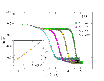
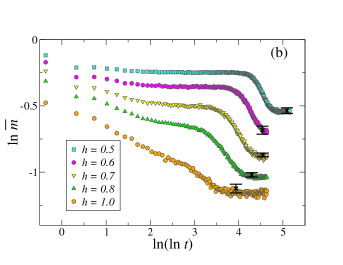
Figure 1: Relaxation of the average magnetization after a quench from a fully ordered state to states within the ferromagnetic phase. (a) Relaxation for different system sizes with the final parameter of the transverse field $h=0.5$; the largest error in these data sets is given by the error bar (black). The inset shows the delay time $t_{d}$ when the inflection point of the second decay occurs, as a function of the system size $L$; the slope of the straight line is $0.94$. (b) Relaxation in a chain of length $L=128$ to final states with various values of $h<1$ in the ferromagnetic phase and also with the critical value $h=h_{c}=1$; the first plateau seen in the data for quenches to a ferromagnetic phase with small $1-h$ is smeared out as the final state approaches the critical point with $h=1$. The largest errors in each data set are indicated by the error bars.

Before we study quenches to the critical point, we first consider the situation in which the system is quenched to a state within the ferromagnetic state with $h<1$. In figure 1(a) we present the time dependence of the average magnetization after a quench to $h=0.5$ for different chain lengths from $L=16$ to $L=128$. As seen in this figure, there is first a decay, followed by a plateau extending to time $t_{d}$, after which ($t>t_{d}$) the magnetization decays sharply before it saturates at a second plateau; the delay time $t_{d}$ is $L$-dependent and scales approximately as $\ln(\ln t_{d})\approx\ln L+\mathrm{const}$, as shown in the inset of figure 1(a). Similar characteristics is observed for other values of $h<h_{c}$ (shown in figure 1(b)) when the final state is within the ferromagnetic phase.

To explain the behavior observed in figure 1 we recall that according to a semiclassical theory [36, 18, 41, 42] the local magnetization at a given site decreases in time if an odd number of quasi-particles, created by the quench, pass through the site. In a random chain the motion of the quasi-particles is limited within a finite localization length $\xi_{\mathrm{loc}}(h)$, which depends on $h$ and grows as the critical point is approached; thus the decay of the magnetization stops at some point of time when the travel distance of the quasi-particles is reached, which explains the presence of the first plateau and why this plateau is smeared out when $h$ approaches the critical point (figure 1(b)). The second decay of the magnetization is related to the lowest excitation. In the ferromagnetic phase, the lowest energy gap vanishes exponentially with the system size as $\epsilon_{0}(L)\sim\exp(-L/\xi)$, $\xi$ being the correlation length, thus the corresponding time scale $t_{d}\sim 1/\epsilon_{0}$ grows exponentially with $L$, as shown in the inset of figure 1(a). At the critical point, the lowest excitation vanishes as $\epsilon_{0}(L)\sim\exp(-AL^{1/2})$ (see (9)); thus, different relaxation behavior is expected for a quench to the critical point and this is discussed in the following subsection.

3.1.2 Critical final state

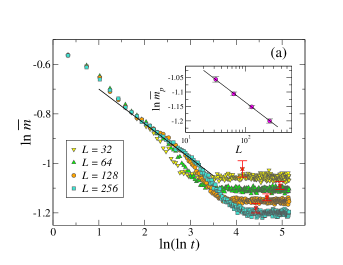
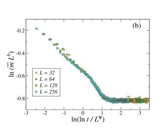
Figure 2: Relaxation of the magnetization after a quench from a fully ordered state to the critical point. (a) The straight line indicating the decay in the transient region has a slope $a=0.14$. The long-time limiting values as a function of $L$ are shown in the inset in a log-log plot; the slope of the straight line is given by $b=0.069$. The largest errors in each data set are given by the error bars (red). (b) A scaling plot of the data in (a), with the parameters $b=0.069$ and $\psi=0.5$.

Relaxation of the average magnetization from the fully ordered initial state to the critical point is shown in figure 2 for various chain lengths. Here the first plateau observed in a ferromagnetic final state is missing, and instead there is a transient region showing a linear relation between $\ln\overline{m}(t)$ and $\ln(\ln t)$ with a slope $a\approx 0.14$, corresponding to a logarithmically show decay:

$$\overline{m}(t)\sim(\ln t)^{-a}\;.$$ (14)

This transient regime terminates at a delay time, $t_{d}(L)$, which is an increasing function of $L$. For $t>t_{d}(L)$ the magnetization decays faster and then saturates to a plateau with large-time limiting value $\overline{m_{p}}(L)$, which has a power-law $L$-dependence as

$$\overline{m_{p}}(L)\sim L^{-b}\;;$$ (15)

the exponent $b$ is estimated as $b\approx 0.069$ in the inset of figure 2(a). Since the two expressions in (14) and (15) should match at $t=t_{d}(L)$, we arrive at the relation: $\ln t_{d}(L)\sim L^{b/a}$. Comparing with (3), we have $\psi_{\mathrm{ne}}=b/a$, agreeing, within error bars, with the RSRG-X prediction: $\psi_{\mathrm{ne}}=\psi=0.5$. This result is illustrated in figure 2(b) in which the scaled magnetization, $L^{b}\overline{m}(t)$ is plotted against the scaling combination $\ln t/L^{\psi}$; with the exponents measured in figure 2(a) we obtain an excellent scaling collapse. Here we comment on the logarithmic decay described in (14). A similar logarithmic decay is also present in the XX-chain with bond disorder, where a larger exponent $a=2$ is found [90, 87]. The critical states of the random-bond XX-chain and the random transverse-field Ising chain are both governed by an infinite-randomness fixed point in SDRG language. The slower decay (corresponding to a smaller exponent $a$) for the random transverse-field Ising chain is due to effective spin clusters formed during renormalization. In the semi-classical picture [42], relaxation of the order parameter is contributed by quasi-particles created during the quench; a spin is flipped if the trajectory of a quasi-particle crosses the given site at a later time. For the relaxation of a larger cluster more quasi-particles are needed, which takes more time. The magnetic moment of an effective spin cluster of the random transverse-field Ising chain scales as $\mu\sim L^{d_{f}}$, with a fractal dimension $d_{f}>0$. The process of formation of spin clusters is missing in the SDRG procedure for the XX-chain, where only random singlets are formed, corresponding to $d_{f}=0$. The different SDRG procedures for the Ising chain and the XX-chain lead to different functional forms of the decay.

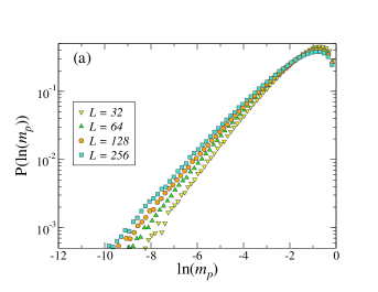
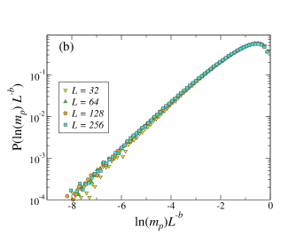
Figure 3: (a) Distribution of the large-time limiting values $m_{p}$ of the dynamical magnetization after a quench from a fully ordered state to the critical point for different chain lengths $L$. (b) A scaling plot for the data in (a) with $b=0.069$.

In a random system the distributions of some observables are also of interest. Here we focus on the distributions of the large-time limiting values $m_{p}$ of the magnetization. In figure 3(a) we plot the distribution of the logarithmic values $\ln(m_{p})$ for $t\gtrsim\exp(\exp(4.5))$ for different system sizes. The distribution of the logarithmic variable is broad and becomes broader with increasing $L$. A good scaling collapse can be obtained in terms of the scaled variable $y=\ln(m_{p})L^{-\alpha}$, thus

$$P_{L}(\ln m_{p})=L^{-\alpha}\tilde{P}\bigl{(}\ln(m_{p})L^{-\alpha}\bigr{)}\;,$$ (16)

as illustrated in figure 3(b), with an estimated exponent $\alpha=0.069$ equaling the exponent $b$ in (15) for the scaling of the average value. Furthermore, the typical value $m_{p}^{\mathrm{typ}}$ is exponentially small and scales as $m_{p}^{\mathrm{typ}}\sim\exp(-CL^{\alpha})$, where $C$ is a constant; comparing with the average value in (15), it is then obvious that the average value is determined by rare events (or samples), in which the large-time limiting value of the magnetization is $m_{p}(L)={\cal O}(1)$. Consequently, the average value of $m_{p}(L)$ is determined by the behavior of the distribution function in the limit of $y\to 0^{-}$, which is assumed to be in a power-law form:

$$\tilde{P}(y)\sim(-y)^{\chi}\;,$$ (17)

with $\chi=0$ in our case shown in figure 3(b). The average of $m_{p}$ is then given by

$$\overline{m_{p}} = L^{-\alpha}\int{\rm d}m_{p}\,\tilde{P}\bigl{(}\ln(m_{p})L^{-\alpha}\bigr{)}$$ (18)

$$\sim L^{-\alpha}\int{\rm d}m_{p}\,\bigl{[}\ln(m_{p})L^{-\alpha}\bigr{]}^{\chi}\sim L^{-\alpha(1+\chi)}\;;$$

thus, with $\alpha=b$ and $\chi=0$ we recover the relation $\overline{m_{p}}\sim L^{-b}$, as given in (15).

3.2 Relaxation from a fully disordered initial state

Now we turn to the case in which the system is quenched from a fully disordered initial state ($h_{0}=\infty$) to the critical point ($h=1$).

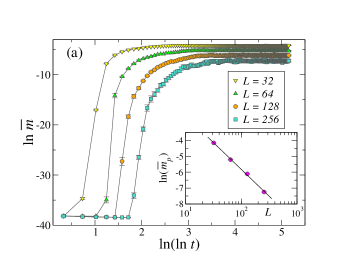
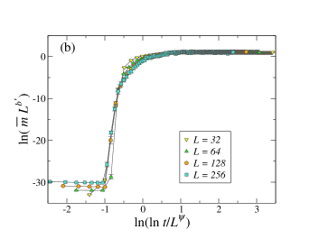
Figure 4: (a) Time-dependent average magnetization in finite chains after a quench from a fully disordered state to the critical point. In the inset the large-time limiting values are shown as a function of $L$ in a log-log plot. The slope of the straight line is given by $b^{\prime}=1.46$. (b) A scaling plot of the data in (a) with the parameters $b^{\prime}=1.46$ and $\psi=0.5$.

Looking at the time-dependent average magnetization for various system sizes plotted in figure 4(a), there is a period of time $0<t<t_{d}(L)$ just after the quench where the magnetization stays negligible and practically corresponds to the initial magnetization before the quench. After this delay time $t_{d}$, which is $L$-dependent, the average magnetization starts to increase rapidly and in the large-time limit it approaches a plateau, the value of which has a power-law $L$-dependence:

$$\overline{m_{p}}(L)\sim L^{-b^{\prime}}\;,$$ (19)

with $b^{\prime}=1.46$, as measured in the inset of figure 4(a). Using the scaled variables $\overline{m}L^{b^{\prime}}$ and $\ln t/L^{\psi}$, we achieve a good data collapse for the time-dependent magnetization in the scaling plot shown in figure 4(b). The increase of the average magnetization in the disordered chain after the quench is unexpected since semiclassical theory predicts a monotonous decrease of the dynamical magnetization in a homogeneous system.

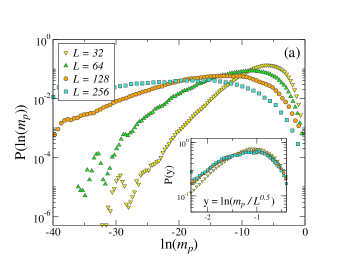
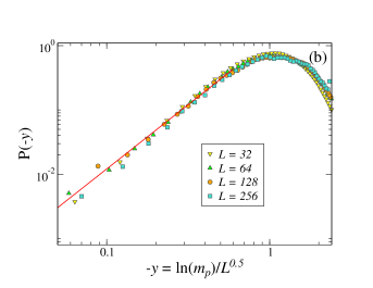
Figure 5: (a) Distribution of the large-time limiting values of the dynamical magnetization after a quench from a fully disordered state to the critical point calculated for different chain lengths; inset: a scaling plot, assuming $\ln m_{p}\sim L^{\alpha^{\prime}}$ with $\alpha^{\prime}=0.5$. (b) The asymptotic behavior of the scaled distribution in terms of $y=\ln m_{p}/\sqrt{L}$ in the limit of $y\to 0^{-}$. The red solid line corresponds to $P(y)\sim(-y)^{2}$.

To understand the mechanism behind the increase of the average magnetization, we have studied the distribution of the large-time limiting values $m_{p}(L)$, which is presented in figure 5(a). The distribution is extremely broad even on the logarithmic scale and it gets broader with increasing system size; in terms of a scaling combination $y=\ln m_{p}L^{-\alpha^{\prime}}$ with $\alpha^{\prime}=0.5$, the inset of figure 5(a) shows a scaling plot with good data collapse. We can then conclude that the typical value scales with $L$ as $m_{p}^{\mathrm{typ}}\sim\exp(-C\,L^{\alpha^{\prime}})$ and is much smaller than the average given in (19). Thus also in this quench process the average value is determined by rare events, in which the large-time limiting values of the magnetization are $m_{p}(L)={\cal O}(1)$. Similar to the situation for a quench from an ordered state as discussed in section 3.1, we have found a power-law form $\tilde{P}(y)\sim(-y)^{\chi^{\prime}}$ for $y\to 0^{-}$ with an estimated exponent $\chi^{\prime}=2.0$ (shown in figure 5(b)). Thus, we have found the size-dependence of the average magnetization in (18) as $\overline{m_{p}}(L)\sim L^{-\alpha^{\prime}(1+\chi^{\prime})}=L^{-1.5}$, which agrees with (19) within the error bars.

The scaling behavior of the large-time limiting value of the dynamical order parameter can be better understood if the boundary site ($l=1$) of an open chain is considered. The large-time limiting value of the surface magnetization, $m_{p}^{s}$, can be exactly calculated (see equation (16) in Ref. [78]):

$$m_{p}^{s}=\Phi_{1}(1)\sum_{j=1}^{L}\Phi_{1}(j)\Phi_{1}^{(0)}(j)\;.$$ (20)

Here:

$$\Phi_{1}(j) = \Phi_{1}(1)\prod_{i=1}^{j-1}\frac{h_{i}}{J_{i}}\,,$$

$$\Phi_{1}(1) = \left[1+\sum_{l=1}^{L-1}\prod_{j=1}^{l}\left(\frac{h_{j}}{J_{j}}\right)^{2}\right]^{-1/2}\,.$$ (21)

For $\Phi_{1}^{(0)}(j)$ in the large-$h_{0}$ limit we have $\Phi_{1}^{(0)}(j)=\delta_{l_{m},j}$, where $l_{m}$ is the position of the largest transverse field in the sample [99]. Thus

$$m_{p}^{s}=[\Phi_{1}(1)]^{2}\prod_{j=1}^{l_{m}-1}\left(\frac{h_{j}}{J_{j}}\right)\;,$$ (22)

where $\Phi_{1}(1)=m^{s}_{\mathrm{eq}}$ is the equilibrium value of the surface magnetization of the chain [100, 101], evaluated in the final state, i.e. with $h=h_{c}$. It is known that the typical value of $m^{s}_{\mathrm{eq}}$ at the critical point scales as $\exp(-CL^{1/2})$ [101, 102] and the same scaling form holds for $m_{p}^{s}$; thus the proper scaling combination for $m_{p}^{s}$ is $y=\ln(m_{p}^{s})L^{-1/2}$, which in the same form for bulk spins discussed above. Concerning the scaling behavior of the average value $\overline{m_{p}^{s}}$, it is dominated by rare events. As described in Ref. [101], there is a close analogy between the random transverse-field Ising chain and a one-dimensional random walk: to a given sample with a set of couplings $J_{i}$, and transverse fields $h_{i}$, $i=1,2,\dots L$, one can assign a one-dimensional random walk which starts at the origin and takes consecutive steps, the length of the $i$-th step being $\ln(h_{i}/J_{i})$. For a rare realization of $m^{s}_{\mathrm{eq}}$, the associated random walk has a surviving character, i.e. it stays at positive position for all steps. Concerning $m_{p}^{s}$, here for a rare realization both $m^{s}_{\mathrm{eq}}$ and the product $\prod_{j=1}^{l_{m}-1}\left(\frac{h_{j}}{J_{j}}\right)$ should be of order of ${\cal O}(1)$; in the language of random walks, this means that the walk is surviving and returns after $l_{m}$ steps. This particular event has the probability: ${\cal P}(l_{m})\sim l_{m}^{-3/2}(L-l_{m})^{-1/2}$ and its average value scale as: $\sum_{l_{m}}{\cal P}(l_{m})/L\sim L^{-3/2}$, which means that $\overline{m_{p}^{s}}(L)\sim L^{-3/2}$. The numerically observed scaling behavior for the bulk magnetization in (19) is similar to this form.

4 Conclusions

In this paper we have studied numerically the time dependent magnetization of the random transverse-field Ising chain after a quench. In order to obtain accurate numerical results we have mainly performed matrix product operations with multiple precision arithmetics in our calculations, instead of any eigenvalue solver routine. In this way we obtained our finite-size results up to length $L=256$ free from numerical instability. We note that some problems with numerical instability using eigenvalue solvers occurred when studying the entanglement entropy in large systems like $L=256$ [84, 87].

For a quench from a fully ordered initial state to a state within the ferromagnetic phase, the average magnetization is shown to relax first to a plateau value, followed by a second relaxation after a delay time $t_{d}\sim\exp(cL)$ to a second plateau value. This second relaxation is attributed to quasi-localized modes which are present in finite systems in the ferromagnetic phase. Both plateau values are $h$-dependent, and finite because in the free-fermionic picture the emitted quasi-particles are localized and travel only a finite distance, which reduces the initial order parameter by a finite fraction only. This behavior is similar to that observed in the Aubry-André model when the quench is performed to the localized phase [79].

When the system is quenched from a fully ordered initial state to the critical finale state, the relaxation of the average magnetization is logarithmically slow (see (14)), and the large-time limiting value decays as a power of $L$ (see (15)). Between the time scale ($t$) and the length scale ($L$) we have found the same relation as in equilibrium, $\ln t\sim\sqrt{L}$, as predicted by the RSRG-X approach [89, 90, 91]. We have also studied the distribution of large-time limiting values of the magnetization: the typical value decreases exponentially with the system size as $\exp(-CL^{\alpha})$, more rapidly than the average value, which decays as a power-law and is determined by rare realizations. The relaxation process after the quench can be explained by the diffusion of quasi-particles in a random environment; the travel distance ($\ell$) of the quasi-particles within time $t$ scales like $\ln(t)\sim\sqrt{\ell}$.

In a quench process from a fully disordered initial state to the critical point, one observes a delay time, $t_{d}\sim\exp(CL^{1/2})$, in which the average magnetization is negligible, and for $t>t_{d}$ a rapid increase of the average magnetization toward an asymptotic large-time limiting value, which has a power-law $L$-dependence (see (19)). The distribution of the large-time limiting magnetizations shows that the typical and the average values scale differently, and the average is determined by rare events. Qualitatively and even quantitatively similar behavior is found for the time dependence of the surface magnetization, which has exact scaling arguments. It has been explicitly shown that there are rare samples, in which after a delay time a stationary surface magnetization of order of ${\cal O}(1)$ develops. These rare samples will then dominate the average value. Such a phenomenon is similar to phase ordering dynamics in classical systems [103], but not expected in closed homogeneous quantum systems.

Appendix A Time evolution of Majorana operators in quadratic fermionic systems

Let us consider a general Hamiltonian, $\cal H$, which is quadratic in terms of fermion creation, $c_{k}^{{\dagger}}$, and annihilation, $c_{k}$, operators and is given for $t>0$ as:

$${\cal H}=\sum_{k,l=1}^{L}\left[c_{k}^{{\dagger}}{A}_{kl}c_{l}+\frac{1}{2}\left(c_{k}^{{\dagger}}{B}_{kl}c_{l}^{{\dagger}}+{\rm h.c.}\right)\right]\;.$$ (23)

Here ${A}_{kl}\equiv(\mathbf{A})_{kl}={A}_{lk}$ and ${B}_{kl}\equiv(\mathbf{B})_{kl}=-{B}_{lk}$ are real numbers, and $k,l$ are the sites of a lattice. In the initial state, i.e. for $t<0$, the parameters of the initial Hamiltonian (${\cal H}^{(0)}$) are different, say ${A}_{kl}^{(0)}$ and ${B}_{kl}^{(0)}$, and the ground state of the initial Hamiltonian is denoted by $|\Psi_{0}^{(0)}\rangle$.

For $t>0$ the Heisenberg equation of motion for the operators $c_{k,H}(t)$ and $c_{k,H}^{{\dagger}}(t)$ are given by $\frac{\rm d}{{\rm d}t}c_{k,H}^{({\dagger})}(t)=\imath[{\cal H},c_{k,H}^{({\dagger})}(t)]$, i.e.

$$\frac{\rm d}{{\rm d}t}c_{k,H}(t)=-\imath\sum_{l}[A_{kl}c_{l,H}(t)+B_{kl}c^{{\dagger}}_{l,H}(t)]\,,$$

$$\frac{\rm d}{{\rm d}t}c^{{\dagger}}_{k,H}(t)=\imath\sum_{l}[A_{kl}c^{{\dagger}}_{l,H}(t)+B_{kl}c_{l,H}(t)]\,,$$ (24)

which are linear since ${\cal H}$ is quadratic. For the Majorana fermion operators $\check{a}_{2k-1}$ and $\check{a}_{2k}$ at site $k$ as defined in (5) the time evolution is given by:

$$\frac{\rm d}{{\rm d}t}\check{a}_{2k-1}(t)=-\sum_{l}[A_{kl}-B_{kl}](t)]\check{a}_{2l}(t)\;,$$

$$\frac{\rm d}{{\rm d}t}\check{a}_{2k}(t)=\sum_{l}[A_{kl}+B_{kl}](t)]\check{a}_{2l-1}(t)\;,$$ (25)

which can be rewritten as

$$\frac{\rm d}{{\rm d}t}\check{a}_{m}(t)=-\sum_{n=1}^{2L}M_{mn}\check{a}_{n}(t)\;.$$ (26)

with a $2L\times 2L$ antisymmetric matrix ${\bf M}$ defined by

$$M_{2k-1,2l} = -M_{2l,2k-1}=-(A_{kl}-B_{kl})\;,$$

$$M_{2k,2l} = M_{2l-1,2k-1}=0\;.$$ (27)

The time dependent Majorana operators are related to the initial operators through

$$\check{a}_{m}(t)=\sum_{n=1}^{2L}P_{mn}(t)\check{a}_{m}(0)\;,$$ (28)

with $P_{mn}(0)=\delta_{mn}$. Inserting (28) into (26) we obtain a set of differential equations for the time evolution of the parameters:

$$\frac{{\rm d}P_{mn}(t)}{{\rm d}t}=\sum_{k=1}^{2L}M_{mk}P_{kn}(t);,$$ (29)

with the initial condition $P_{mn}(0)=\delta_{mn}$. The solution as a shorthand matrix notation is given in (11), in which the exponential can be evaluated by using the spectral decomposition of ${\bf M}$. Indeed, the eigenvalues of ${\bf M}$ are given by the energies of the free-fermionic modes of ${\cal H}$ in (23), which can be seen by forming ${\bf M}^{2}$ and comparing it with the results in Ref. [92] . Details of the calculation using the spectral decomposition of ${\bf M}$ are presented in the appendix of Ref. [78].

References

References

- [1] Greiner M, Mandel O, Hänsch T W, and Bloch I 2002 Nature 419 51
- [2] Paredes B et al. 2004 Nature 429 277
- [3] Kinoshita T, Wenger T and Weiss D S 2004 Science 305 1125
- [4] Sadler L E, Higbie J M, Leslie S R, Vengalattore M, and Stamper-Kurn D M 2006 Nature 443 312
- [5] Lamacraf A 2006 Phys. Rev. Lett. 98 160404
- [6] Kinoshita T, Wenger T and Weiss D S 2006 Nature 440 900
- [7] Hofferberth S, Lesanovsky I, Fischer B, Schumm T, and Schmiedmayer J 2007 Nature 449 324
- [8] For a review see: Bloch I, Dalibard J and Zwerger W 2008 Rev. Mod. Phys. 80 885
- [9] Trotzky S, Chen Y-A, Flesch A, McCulloch I P, Schollwöck U Eisert J, and Bloch I 2012 Nature Phys. 8 325
- [10] Cheneau M, Barmettler P, Poletti D, Endres M, Schauss P, Fukuhara T, Gross C, Bloch I, Kollath C and Kuhr S 2012 Nature 481 484
- [11] Gring M, Kuhnert M, Langen T, Kitagawa T, Rauer B, Schreitl M, Mazets I, Smith D A, Demler E and Schmiedmayer J 2012 Science 337 1318
- [12] Polkovnikov A, Sengupta K, Silva A, and Vengalattore M 2011 Rev. Mod. Phys. 83 863
- [13] Barouch E and McCoy B 1970 Phys. Rev. A 2 10751971 Phys. Rev. A 3 7861071 Phys. Rev. A 3 2137
- [14] Iglói F and Rieger H 2000 Phys. Rev. Lett. 85 3233
- [15] Sengupta K, Powell S and Sachdev S 2004 Phys. Rev. A 69 053616
- [16] Rigol M, Dunjko V, Yurovsky V and Olshanii M 2007 Phys. Rev. Lett. 98 50405 Rigol M, Dunjko V and Olshanii M 2008 Nature 452 854
- [17] Calabrese P and Cardy J 2006 Phys. Rev. Lett. 96 136801
- [18] Calabrese P and Cardy J 2007 J. Stat. Mech. P06008
- [19] Cazalilla M A 2006 Phys. Rev. Lett. 97 156403Iucci A and Cazalilla M A 2010 New J. Phys. 12 055019Iucci A and Cazalilla M A 2009 Phys. Rev. A 80 063619
- [20] Manmana S R, Wessel S, Noack R M and Muramatsu A 2007 Phys. Rev. Lett. 98 210405
- [21] Cramer M, Dawson C M, Eisert J and Osborne T J 2008 Phys. Rev. Lett. 100 030602Cramer M and Eisert J 2010 New J. Phys. 12 055020Cramer M, Flesch A, McCulloch I A, Schollwöck U and Eisert J 2008 Phys. Rev. Lett. 101 063001Flesch A, Cramer M, McCulloch I P, Schollwöck U and Eisert J 2008 Phys. Rev. A 78 033608
- [22] Barthel T and Schollwöck U 2008 Phys. Rev. Lett. 100 100601
- [23] Kollar M and Eckstein M 2008 Phys. Rev. A 78 013626
- [24] Sotiriadis S, Calabrese P and Cardy J 2009 EPL 87 20002
- [25] Roux G 2009 Phys. Rev. A 79 021608Roux G 2010 Phys. Rev. A 81 053604
- [26] Sotiriadis S, Fioretto D and Mussardo G 2012 J. Stat. Mech. P02017Fioretto D and Mussardo G 2010 New J. Phys. 12 055015Brandino G P, De Luca A, Konik R M, and Mussardo G 2012 Phys. Rev. B 85 214435
- [27] Kollath C, Läuchli A and Altman E 2007 Phys. Rev. Lett. 98 180601Biroli G, Kollath C and Läuchli A 2010 Phys. Rev. Lett. 105 250401
- [28] Banuls M C, Cirac J I, and Hastings M B 2011 Phys. Rev. Lett. 106 050405
- [29] Gogolin C, Müller M P and Eisert J 2011 Phys. Rev. Lett. 106 040401
- [30] Rigol M and Fitzpatrick M 2011 Phys. Rev. A 84 033640
- [31] Caneva T, Canovi E, Rossini D, Santoro G E and Silva A 2011 J. Stat. Mech. P07015
- [32] Rigol M and Srednicki M 2012 Phys. Rev. Lett. 108 110601
- [33] Santos L F, Polkovnikov A and Rigol M 2011 Phys. Rev. Lett. 107 040601
- [34] Grisins P and Mazets I E 2011 Phys. Rev. A 84 053635
- [35] Canovi E, Rossini D, Fazio R, Santoro G E and Silva A 2011 Phys. Rev. B 83 094431
- [36] Calabrese P and Cardy J 2005 J. Stat. Mech. P04010
- [37] Fagotti M and Calabrese P 2008 Phys. Rev. A 78 010306
- [38] Silva A 2008 Phys. Rev. Lett. 101 120603Gambassi A and Silva A 2012 Phys. Rev. Lett. 109 250602
- [39] Rossini D, Silva A, Mussardo G and Santoro G 2009 Phys. Rev. Lett. 102 127204Rossini D, Suzuki S, Mussardo G, Santoro G E and Silva A 2010 Phys. Rev. B 82 144302
- [40] Campos Venuti L and Zanardi P 2010 Phys. Rev. A 81 022113Campos Venuti L, Jacobson N T, Santra S and Zanardi P 2011 Phys. Rev. Lett. 107 010403
- [41] Iglói F and Rieger H 2011 Phys. Rev. Lett. 106 035701
- [42] Rieger H and Iglói F 2011 Phys. Rev. B 84 165117
- [43] Foini L, Cugliandolo L F and Gambassi A 2011 Phys. Rev. B 84 212404Foini L, Cugliandolo L F and Gambassi A 2012 J. Stat. Mech. P09011
- [44] Calabrese P, Essler F H L and Fagotti M 2011 Phys. Rev. Lett. 106 227203
- [45] Schuricht D and Essler F H L 2012 J. Stat. Mech. P04017
- [46] Calabrese P, Essler F H L and Fagotti M 2012 J. Stat. Mech. P07016Calabrese P, Essler F H L and Fagotti M 2012 J. Stat. Mech. P07022
- [47] Blaß B, Rieger H and Iglói F 2012 EPL 99 30004
- [48] Essler F H L, Evangelisti S, Fagotti M 2012 Phys. Rev. Lett. 109 247206
- [49] Evangelisti S 2013 J. Stat. Mech. P04003
- [50] Fagotti M 2013 Phys. Rev. B 87 165106
- [51] Pozsgay B 2013 J. Stat. Mech. P07003Pozsgay B 2013 J. Stat. Mech. P10028
- [52] Fagotti M, Essler F H L 2013 J. Stat. Mech. P07012
- [53] Collura M, Sotiriadis S and Calabrese P 2013 J. Stat. Mech. P09025
- [54] Bucciantini L, Kormos M, Calabrese P 2014 J. Phys. A: Math. Theor. 47 175002
- [55] Fagotti M, Collura M, Essler F H L and Calabrese P 2014 Phys. Rev. B 89 125101
- [56] Cardy J 2014 Phys. Rev. Lett. 112 220401
- [57] Wouters B, Brockmann M, De Nardis J and Fioretto D, Rigol M and Caux J S 2014 Phys. Rev. Lett. 113 117202
- [58] Pozsgay B, Mestyán M, Werner M A, Kormos M, Zaránd G, Takács G 2014 Phys. Rev. Lett. 113 117203
- [59] Goldstein G and Andrei N 2014 Phys. Rev. A 90 043625
- [60] Pozsgay B 2015 J. Stat. Mech. P09026
- [61] Pozsgay B 2015 J. Stat. Mech. P10045
- [62] Larson J 2013 J. Phys. B: At. Mol. Opt. Phys. 46 224016
- [63] Hamazaki R, Ikeda T N and Ueda M 2016 Phys. Rev. E 93 032116
- [64] Blaß B and Rieger H 2016 arXiv:1605.06258
- [65] Essler F H L, Mussardo G and Panfil M 2015 Phys. Rev. A 91 051602
- [66] Ilievski E, De Nardis J, Wouters B, Caux J S, Essler F H L, Prosen T 2015 Phys. Rev. Lett. 115 157201
- [67] Ilievski E, Medenjak M, Prosen T, Zadnik L 2016 J. Stat. Mech. Theor. Exp. P064008
- [68] Doyon B 2015 arXiv:1512.03713.
- [69] Vidmar L, Rigol M 2016 J. Stat. Mech. Theor. Exp. P064007
- [70] Peschel I 2003 J. Phys. A: Math. Gen. 36 L205
- [71] Peschel I and Zhao J 2005 J. Stat. Mech. P11002
- [72] Levine G C and Miller D J 2008 Phys. Rev. B 77 205119
- [73] Iglói F, Szatmári Z and Lin Y-C 2009 Phys. Rev. B 80 024405
- [74] Eisler V and Peschel I 2010 Ann. Phys. (Berlin) 522 679
- [75] Calabrese P, Mintchev M and Vicari E 2012 J. Phys. A: Math. Theor. 45 105206
- [76] Peschel I and Eisler V 2012 J. Phys. A: Math. Theor. 45 155301
- [77] Iglói F, Juhász R and Zimborás Z 2007 Europhys. Lett. 79 37001
- [78] Iglói F, Roósz G and Lin Y-C 2013 New J. Phys. 15 023036
- [79] Roósz G, Divakaran U, Rieger H and Iglói F 2014 Phys. Rev. B 90 184202
- [80] Anderson P W 1958 Phys. Rev. 109 1492
- [81] Basko D M, Aleiner I L and Altshuler B L 2006 Annals of Physics 321 1126
- [82] Huse D A, Nandkishore R, Oganesyan V 2014 Phys. Rev. B 90 174202
- [83] De Chiara G, Montangero S, Calabrese P and Fazio R 2006 J. Stat. Mech. L03001
- [84] Iglói F, Szatmári Z and Lin Y-C 2012 Phys. Rev. B 85 094417
- [85] Levine G C, Bantegui M J, Burg J A 2012 Phys. Rev. B 86 174202
- [86] Bardarson J H, Pollmann F and Moore J E 2012 Phys. Rev. Lett. 109 017202
- [87] Zhao Y, Andraschko F and Sirker J 2016 Phys. Rev. B 93 205146
- [88] For a review, see: Iglói F and Monthus C 2005 Physics Reports 412 277
- [89] Pekker D, Refael G, Altman E, Demler E and Oganesyan V 2014 Phys. Rev. X 4 011052
- [90] Vosk R and Altman E 2013 Phys. Rev. Lett. 110 067204
- [91] Vosk R and Altman E 2014 Phys. Rev. Lett. 112 217204
- [92] Lieb E, Schultz T and Mattis D 1961 Ann. Phys. (N.Y.) 16 407
- [93] Pfeuty P 1970 Ann. Phys. (Paris) 57 79
- [94] Jordan P and Wigner E 1928 Z. Phys. 47 631
- [95] Yang C N 1952 Phys. Rev. 85 808
- [96] Fisher D S 1992 Phys. Rev. Lett. 69 534Fisher D S 1995 Phys. Rev. B 51 6411
- [97] Fisher D S 1999 Physica A 263 222
- [98] Deylon F, Kunz H, Souillard B 1986 J. Phys. A: Math. Gen. 16 25. Here eigenvalues of the operator are the same as those of .
- [99] It can be seen in Ref.[101], by solving the eigenvalue problem in Eq. (2.2) with , .
- [100] Peschel I 1984 Phys. Rev. B 30 6783
- [101] Iglói F and Rieger H 1998 Phys. Rev. B 57 11404
- [102] Monthus C 2004 Phys. Rev. B 69 054431
- [103] Bray A J 1994 Adv. Phys. 43 357