Model Confidence Bounds for Variable Selection

Summary

In this article, we introduce the concept of model confidence bounds (MCB) for variable selection in the context of nested models. Similarly to the endpoints in the familiar confidence interval for parameter estimation, the MCB identifies two nested models (upper and lower confidence bound models) containing the true model at a given level of confidence. Instead of trusting a single selected model obtained from a given model selection method, the MCB proposes a group of nested models as candidates and the MCB’s width and composition enable the practitioner to assess the overall model selection uncertainty. A new graphical tool — the model uncertainty curve (MUC) — is introduced to visualize the variability of model selection and to compare different model selection procedures. The MCB methodology is implemented by a fast bootstrap algorithm that is shown to yield the correct asymptotic coverage under rather general conditions. Our Monte Carlo simulations and real data examples confirm the validity and illustrate the advantages of the proposed method.

Keywords: Confidence set; Model selection; Uncertainty.

1 Introduction

Variable selection is an important and well-studied topic. Modern analysis is often aimed at selecting a subset of variables from a large number of predictors while attempting to attenuate possible modeling bias. In the context of linear models, a wealth of methods have been introduced to enhance predictability and to select significant predictors. These include popular sparsity-inducing penalization methods such as Lasso (Tibshirani, 1996), SCAD (Fan and Li, 2001), Adaptive Lasso (Zou, 2006) and so on. For an overview of existing methods, please see Fan and Lv (2010).

Regardless of the selection procedure used, variable selection uncertainty is an important and ubiquitous aspect of the model selection activity. Often using the same variable selection method on different samples from a common population results in different models. Even for a single sample, different variable selection methods tend to select different sets of variables in the presence of pronounced noise. Motivated by the need to address this model ambiguity, there has been growing interest in developing model confidence set (MCS) methods, which may be broadly regarded as frequentist approaches for obtaining a set of models statistically equivalent to a true model at a certain level of confidence $100(1-\alpha)\%$. An MCS extends the familiar notion of confidence intervals to the model selection framework and enables one to assess the uncertainty associated with a given selection procedure. If the data are informative, the MCS contains only a few models (exactly one model in the case of overwhelming information), while uninformative data correspond to a large MCS.

Hansen et al. (2011) propose constructing an MCS from a given set of candidate models by a sequence of equivalence tests on the currently remaining models, followed by an elimination rule to remove the worst model. Their method obtains a subset of the original models that is meant to contain (or equal) the set of models with the best performance under some given loss function. Ferrari and Yang (2015) introduce the notion of variable selection confidence set (VSCS) for linear regression. While sharing the same motivation with Hansen et al. (2011), their method constructs the MCS by a sequence of F-tests and achieves exact coverage probability for the true model without necessarily relying on a user-defined initial list of models. They show that, without restrictions on the model structure (e.g., sparsity), the size of the VSCS is potentially large, thus reflecting the possible model selection uncertainty. To address this issue, they introduce the notion of lower bound models (LBMs) — i.e., the most parsimonious models that are not statistically significantly inferior to the full model at a given confidence level — and study their properties. Previously, Shimodaira (1998) advocates the use of a set of models that have AIC values close to the smallest among the candidates based on hypothesis testing. Hansen et al. (2003, 2005) apply an MCS procedure in the context of volatility and forecasting models. Samuels and Sekkel (2013) use the MCS to select a subset of models prior to averaging the resulting forecasts.

The methods above yield MCS satisfying a nominal coverage probability for the true model. However, the models contained in the MCS are not constrained in terms of their structures, meaning that models in the MCS may be drastically different in their compositions with no common variables. This poses challenges in interpreting the models in the MCS. In this paper, we introduce a new procedure that computes the so-called model confidence bounds (MCB). The MCB is constructed by finding a large and a small model — called upper bound model (UBM) and lower bound model (LBM), respectively — that are nested and where the true model is included between the two at user-specified confidence level $100(1-\alpha)\%$. The LBM and UBM have a rather natural interpretation: The LBM is regarded as the most parsimonious model containing indispensable predictors, whereas models containing variables beyond the UBM include superfluous predictors. Note that, even though MCS is more general than MCB since it can be applied to non-nested models, these two methods focus on different objectives. MCS aims at prediction accuracy, while MCB focuses on model selection uncertainty and on providing more information and interpretation of the model selection results. It is the similar idea that a confidence interval provides more information than a point estimate.

Our methodology provides a platform for assessing the uncertainty associated with different model selection methods. Just like using the width of the familiar confidence interval to compare different estimator’s uncertainty, the practitioner can decide which model selection method yields more stable results through comparing the widths and compositions of MCB of different methods. The MCB can also be used as a model selection diagnostic tool. If a proposed model is not within the MCB at a certain confidence level, there is a strong reason to doubt the soundness of its predictors. The proposed method is based on bootstrap and may be extended to a wide range of model families. Finally, to calculate the MCB, we first propose an exact but computationally intensive algorithm; we further propose a much more efficient approximated algorithm whose performance is found to be comparable to that of the exact algorithm.

The rest of the paper is organized as follows. In Section 2, we introduce the model confidence bounds (MCB), study its properties, and develop a graphical tool, model uncertainty curve (MUC), to assess model selection uncertainty. In Section 3, we propose fast algorithms to find MCB and study their computational advantages. We apply the proposed method to a real data set in Section 4, and carry out Monte Carlo experiments in Section 5. We give final remarks in Section 6 and relegate the proofs and additional numerical studies to Web Appendices.

2 Methodology

2.1 Preliminaries

We focus on linear regression models. Let $\bm{Y}=(y_{1},...,y_{n})^{T}$ be an $n\times 1$ response vector with mean $\bm{\mu}$. Suppose $\bm{Y}=\bm{X}\bm{\theta}+\bm{\epsilon}$ where $\bm{X}=(\bm{x}_{1},...,\bm{x}_{n})^{T}$ is an $n\times p$ matrix of predictors with the $i$th row vector $\bm{x}_{i}=(x_{i1},...,x_{ip})^{T}\in\mathbb{R}^{p}$, $\bm{\theta}=(\theta_{1},\dots,\theta_{p})^{T}\in\mathbb{R}^{p}$ is the parameter vector, and $\bm{\epsilon}=(\epsilon_{1},...,\epsilon_{n})^{T}\sim N_{n}(\bm{0},\sigma^{2}\bm{I}_{n})$. We further make sparsity assumption and assume some of the elements in $\bm{\theta}$ are zeros, but we do not know which ones. Let $\widehat{m}$ be the index set of some predictors so that it defines a possible model and $\emptyset\subseteq\widehat{m}\subseteq\{1,...,p\}$. Then, we have the following definition:

Definition 1.

Let $m^{\ast}$ be the index set of predictors with non-zero true coefficients, $m^{\ast}=\{j:\theta_{j}\neq 0,j=1,...,p\}$. Let $m_{\textup{full}}$ be the index set of all predictors, $m_{\textup{full}}=\{j:j=1,...,p\}$.

Therefore, $m^{\ast}$ represents the true model, and $m_{\textup{full}}$ represents the full model. Without the loss of generality, we assume that the first $p^{\ast}$ coefficients ($p^{\ast}\leq p$) in $\bm{\theta}$ are different from zero so that the true model is $m^{\ast}=\{1,...,p^{\ast}\}$. Let $\mathcal{M}_{all}=\big{\{}m:\emptyset\subseteq m\subseteq m_{\textup{full}}\big{\}}$ denote the set of all of the possible models. In certain situations, prior information on the model structure enables us to restrict further the set of all possible models $\mathcal{M}_{all}$. For example, in polynomial regression, one would include a certain power of the predictor only if all lower-order terms appeared as well. Another case is when certain predictors are always protected in the sense that they appear in all candidate models.

Because $\widehat{m}$ represents a subset of all predictors, it can be obtained from the variable selection procedure. Here we focus on penalized likelihood selection methods. Specifically, $\widehat{m}=\{j:\widehat{\theta}_{j}\neq 0,1\leq j\leq p\}$ where the estimator $\widehat{\bm{\theta}}$ minimizes a penalized likelihood criterion with the form $\ell_{n}(\bm{\theta})=-2\log L_{n}(\bm{\theta};\bm{Y},\bm{X})+\lambda_{n}R(\bm{\theta})$ where $L_{n}(\bm{\theta};\bm{Y},\bm{X})$ is the likelihood function, $\lambda_{n}\geq 0$ is a user-defined regularization parameter and $R(\bm{\theta})$ is some penalty function $R:\mathbb{R}^{p}\mapsto\mathbb{R}^{+}$. Throughout the paper, $R(\bm{\theta})$ will be a type of norm. For example, $R(\bm{\theta})=\sum_{j=1}^{p}I(\theta_{j}\neq 0)$ corresponds to the $L_{0}$-norm and yields a number of information theoretical selection criteria, including the Akaike information criterion (AIC) for $\lambda=2$, and the Bayesian information criterion (BIC) for $\lambda=\log(n)$. Setting $R(\bm{\theta})=\sum_{j=1}^{p}|\theta_{j}|$ gives the $L_{1}$-norm, which corresponds to Lasso.

2.2 Model Confidence Bounds

For a given sample $D=\{(y_{i},\bm{x}_{i}),i=1,\dots,n\}$, we want to find a small model $\widehat{m}_{L}=\widehat{m}_{L}(D)$ and a large model $\widehat{m}_{U}=\widehat{m}_{U}(D)$ such that the true model $m^{\ast}$ is nested between $\widehat{m}_{L}$ and $\widehat{m}_{U}$ with a probability at least $1-\alpha$ and $\widehat{m}_{L}\subseteq\widehat{m}_{U}$.

Definition 2 (Model Confidence Bounds and Set).

The $100(1-\alpha)\%$-model confidence bounds are defined by the pair of models $\{\widehat{m}_{L},\widehat{m}_{U}\}$ such that

$$P\left(\widehat{m}_{L}\subseteq m^{\ast}\subseteq\widehat{m}_{U}\right)\geq 1-\alpha.$$ (1)

The models $\widehat{m}_{L}$ and $\widehat{m}_{U}$ are called the lower bound model (LBM) and the upper bound model (UBM), respectively. The $100(1-\alpha)\%$-model confidence set (MCS) is defined as $\widehat{\mathcal{M}}_{\alpha}=\{\widehat{m}:\widehat{m}_{L}\subseteq\widehat{m}\subseteq\widehat{m}_{U}\}$. If (1) is valid as $n\rightarrow\infty$, $\{\widehat{m}_{L},\widehat{m}_{U}\}$ define asymptotic model confidence bounds (AMCB) and asymptotic model confidence set (AMCS).

The above definition extends the usual notion of the confidence interval for parameter estimation to the variable selection setting. Similarly to the familiar confidence interval for a population parameter, MCB covers the true model $m^{\ast}$ with a certain probability $1-\alpha$. A model smaller than $\widehat{m}_{L}$ is regarded as too parsimonious in the sense that it is likely to miss at least one important variable, while models with the variables in $\widehat{m}_{U}$ plus other predictors are considered to be overfitting. Similarly to the familiar confidence interval, one can obtain a one-sided $100(1-\alpha)\%$-MCB by setting $\widehat{m}_{L}=\emptyset$ or $\widehat{m}_{U}=m_{\textup{full}}$.

The pair of models $\{\widehat{m}_{L},\widehat{m}_{U}\}$ represent two extreme cases, i.e., the most parsimonious and complex models. Using these two models (i.e., MCB), we can list all possible models nested between those two extremes (i.e., MCS), resulting in an easy-to-interpret hierarchical structure. Moreover, the difference between the $\widehat{m}_{L}$ and $\widehat{m}_{U}$ reflects the model selection uncertainty in a given sample. When the amount of information in the data is very large, $\widehat{m}_{L}$ and $\widehat{m}_{U}$ are very similar, and there are only a few models nested between MCB. In the extreme case of overwhelming information, we have $\widehat{m}_{L}=\widehat{m}_{U}=m^{*}$ and the MCB contains only the true model. In most practical situations, we have $\widehat{m}_{L}\subset\widehat{m}_{U}$, with the discrepancy between $\widehat{m}_{L}$ and $\widehat{m}_{U}$ becoming large when the data are uninformative.

The size of MCB can be measured by the its width which is defined below.

Definition 3 (MCB Width).

Let $w(\widehat{m}_{L},\widehat{m}_{U})=|\widehat{m}_{U}|-|\widehat{m}_{L}|$ be the width associated with the model confidence bounds $\{\widehat{m}_{L},\widehat{m}_{U}\}$, where $|\mathcal{A}|$ represents the cardinality of set $\mathcal{A}$.

Note that there are usually multiple MCBs satisfying Equation (1). Therefore, for simplicity, for any given confidence level $1-\alpha$, we select the MCB which has the shortest width among MCBs satisfying Equation (1) and some additional restriction. We illustrate the selection procedure in details in the following sections.

2.3 Bootstrap Construction of $100(1-\alpha)\%$-MCB

Given the data set $D$, we generate $B$ bootstrap samples $D^{(b)}$, $b=1,\dots,B$. Then we obtain the set of bootstrap models $\mathcal{M}_{boot,B}=\{\widehat{m}^{(b)},b=1,\dots,B\}$ by applying a model selection method to each bootstrap sample $D^{(b)}$. For any two nested models, $m_{1}\subseteq m_{2}$ ($m_{1}$ and $m_{2}$ denote the index sets of some predictors), it seems quite natural to estimate the probability of the event $\{m_{1}\subseteq m^{\ast}\subseteq m_{2}\}$ using the following statistic.

Definition 4.

The bootstrap coverage rate (BCR) of models $m_{1}\subseteq m_{2}$ is $\widehat{r}(m_{1},m_{2})=\sum_{b=1}^{B}I(m_{1}\subseteq\widehat{m}^{(b)}\subseteq m_{2})/B$, where $\widehat{m}^{(1)},\dots,\widehat{m}^{(B)}$ are bootstrap models and $I(\cdot)$ is the indicator function.

For a given confidence level $1-\alpha$, to obtain the LBM and UBM, we need to find a pair of nested models $m_{1}\subseteq m_{2}$ which satisfy the approximate inequality $\widehat{r}(m_{1},m_{2})\geq 1-\alpha$ and have the smallest width $|m_{2}|-|m_{1}|$. To achieve this goal, we first search for the MCB with the highest bootstrap coverage rate at different widths, and subsequently form a sequence of MCBs, $S$. Among the sequence of MCBs, we select the final $100(1-\alpha)\%$-MCB to be the one having the shortest width while maintaining its bootstrap coverage rate greater than or equal to $1-\alpha$. In other words, we solve the following empirical objective function

$$(\widehat{m}_{L},\widehat{m}_{U})=\underset{(m_{1},m_{2})\in S}{\text{argmin}}\left\{|m_{2}|-|m_{1}|:\text{ s.t. }\widehat{r}(m_{1},m_{2})\geq 1-\alpha\right\},$$ (2)

where $S=\{(m_{1}^{(i)},m_{2}^{(i)}),0\leq i\leq p\}$ and $(m_{1}^{(i)},m_{2}^{(i)})=\arg\max_{m_{1},m_{2}}\{\widehat{r}(m_{1},m_{2}):\text{ s.t. }|m_{2}|-|m_{1}|=i,\emptyset\subseteq m_{1}\subseteq m_{2}\subseteq m_{\textup{full}}\}$. The set $S$ represents the sequence of MCBs of different widths whose bootstrap coverage rates are maximized. Therefore, $S$ contains the most representative MCBs at each width. The implementation of this procedure is summarized in Algorithm 1 in Section 3 along with a discussion on computational complexity and improvement. It is clear that this approach works as long as the bootstrap coverage rate estimates consistently the true coverage rate. A more detailed discussion of this issue is deferred to Section 2.5.

2.4 Assessment of Model Selection Uncertainty

Our proposed MCB can be paired with many model selection methods. Therefore, the MCB can be used to assess the uncertainty associated with a given model selection method. Let $\widehat{m}^{(1)},\dots,\widehat{m}^{(B)}$ be bootstrap models under some model selection method. The profiled bootstrap coverage rate (CR) is

$$\text{CR}(w)=\widehat{r}(\widehat{m}_{L},\widehat{m}_{U})=\sum_{b=1}^{B}I(\widehat{m}_{L}\subseteq\widehat{m}^{(b)}\subseteq\widehat{m}_{U})/B,$$ (3)

where $w=|\widehat{m}_{U}|-|\widehat{m}_{L}|$ is the MCB width. Therefore, we treat the CR statistic as a function of the MCB’s width $w$. For an MCB of width $w$, one would like to use $P(\widehat{m}_{L}\subseteq m^{\ast}\subseteq\widehat{m}_{U})$ as a measure of uncertainty for a variable selection method. However, in practice the exact probability is unknown, and instead, the CR statistic is used to approximate $P(\widehat{m}_{L}\subseteq m^{\ast}\subseteq\widehat{m}_{U})$. When a consistent model selection method is used (e.g., BIC, Adaptive Lasso, MCP, SCAD), the $P(\widehat{m}_{L}\subseteq m^{\ast}\subseteq\widehat{m}_{U})$ and the CR are typically very close.

Clearly, a good model selection method would tend to return an MCB with a lower width at a given coverage, or a larger coverage value at a given width. Thus, we propose to assess the uncertainty of a given model-selection mechanism by plotting the pairs of $w/p$ and $\text{CR}(w)$ for all the MCBs in $S$, i.e., $\mathscr{P}_{MUC}=\big{\{}\big{(}w/p,\text{CR}(w)\big{)},\ 0\leq w\leq p\big{\}}$. The resulting plot is called a model uncertainty curve (MUC). Essentially, MUC is formed by $w/p$ and $\text{CR}(w)$ of the entire sequence of MCBs in $S$. Note that $S$ contains the sequence of MCBs of different widths whose bootstrap coverage rates are maximized.

The MUC of a given variable selection method with good performance will tend to arch towards the upper left corner. The MUC is in some sense analogous to that of a receiver operating characteristic (ROC) curve used to assess binary classifiers. The ideal model selection method has $w/p=0$ and $\text{CR}(0)=1$, i.e., no model selection uncertainty at all and perfect coverage (top left corner of the plot). Moreover, the area under the MUC (AMUC) can be used as a raw measure of uncertainty for the variable selection method under examination. A larger value of AMUC implies less uncertainty and more stability of the corresponding variable selection method. Overall, we can decide which method has the best performance according to the shape of the MUC and the corresponding AMUC.

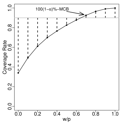
Figure 1: Illustration of MUC and $100(1-\alpha)\%$-MCB with $\alpha=0.1$.

We further present an example of MUC and illustrate its connection to $100(1-\alpha)\%$-MCB. We simulate a data set according to the linear regression $y_{i}=\sum_{j=1}^{p^{\ast}}\theta_{j}x_{ij}+\sum_{j=p^{\ast}+1}^{p}0\times x_{ij}+\epsilon_{i}$ with sample size $n=100$, number of predictors $p=10$, number of true predictors $p^{*}=5$, $\theta_{j}=1$, $\epsilon_{i}\sim N(0,\sigma^{2})$ with $\sigma=3$, and $\bm{x}_{i}\sim N_{p}(\bm{0},\bm{I}_{p})$. We adopt 10-fold cross-validated Adaptive Lasso and plot the MUC in Figure 1. As we can see the MUC arches towards the upper left corner like an ROC curve, which means the model selection method works well for this data set. In addition, on this MUC curve, each bold dot represents the width and coverage rate of one MCB in $S$. It is always true that, for that sequence of MCBs, the coverage rate increases monotonically as the width increases.

Suppose we are given the confidence level $1-\alpha$ (i.e., the nominal coverage probability), we need to select the $100(1-\alpha)\%$-MCB from $S$ (i.e., MUC). In Figure 1, the confidence level is demonstrated by the gray horizontal line. The coverage probability differences (i.e., empirical coverage probability $-$ nominal coverage probability) of each MCB in $S$ are captured by the vertical dashed lines between the dots and horizontal line. Clearly, there is a trade-off between the coverage probability difference and the width. However, because of Definition 2 and Equation 2, only the MCB with nonnegative coverage probability difference is eligible to be the $100(1-\alpha)\%$-MCB. Therefore, all the dots below the gray line are not eligible. In addition, since we are searching for the MCB with the shortest width according to Equation 2, the final $100(1-\alpha)\%$-MCB is the dot closest to and yet above the gray line. The rest of MCBs above the gray line have larger widths compared to the selected $100(1-\alpha)\%$-MCB due to the monotonicity of the coverage rate in width.

2.5 Asymptotic Coverage

The quality of the model selection method can be measured by the underfitting and overfitting probabilities, i.e., the probability of the events $\mathcal{M}^{-}_{n}=\{\widehat{m}\nsupseteq m^{\ast}\}$ and $\mathcal{M}^{+}_{n}=\{\widehat{m}\supsetneqq m^{\ast}\}$. Note that $\mathcal{M}^{-}_{n}$ represents some predictors in the true model are missed. Meanwhile, $\mathcal{M}^{+}_{n}$ represents the predictors in the true model are selected plus some additional superfluous terms. A model selection procedure is consistent if $P(\widehat{m}=m^{\ast})\rightarrow 1$ as $n\rightarrow\infty$ for every $\bm{\theta}\in\mathbb{R}^{p}$, which occurs if $P(\mathcal{M}^{-}_{n})\rightarrow 0$ and $P(\mathcal{M}^{+}_{n})\rightarrow 0$ as $n\rightarrow\infty$. If $P(\mathcal{M}^{-}_{n})\rightarrow 0$ but $\widehat{m}$ is not consistent, then we call the procedure conservative.

Theorem 1.

Assume: (A.1) (Model selection consistency) $P(\mathcal{M}_{n}^{-})=o(1)$ and $P(\mathcal{M}_{n}^{+})=o(1)$; (A.2) (Bootstrap validity). For the re-sampled model $\widehat{m}^{(b)}$, assume $P(\widehat{m}^{(b)}\neq\widehat{m})=o(1)$. Then, for the $\widehat{m}_{L}$ and $\widehat{m}_{U}$ solving program (2), we have $P(\widehat{m}_{L}\subseteq m^{\ast}\subseteq\widehat{m}_{U})\geq 1-\alpha+o(1)$.

The above theorem shows that if the model selection procedure is consistent (i.e., the probability of overfitting or underfitting the underlying model becomes small as the sample size increases), then the CR statistic estimates consistently the true coverage probability associated with models $m_{1}\subseteq m_{2}$. Note that assumptions A.1 and A.2 are common conditions in the literature. For example, Fan and Lv (2010) establish the model selection consistency (as part of the oracle property) as a standard property for many methods. Pötscher and Schneider (2010) and Leeb and Pötscher (2006) have presented similar assumptions in their results. Lastly, Liu and Yu (2013) and Chatterjee and Lahiri (2013) have also stated the bootstrap validity for their methods. For each assumption, we list a few examples as follows.

For Assumption A.1 of model selection consistency, many existing model selection methods are equipped with such a property. In the case of Lasso estimation, Zhao and Yu (2006) establish the condition for selection consistency as the Strong Irrepresentable Condition. This condition can be interpreted as: Lasso estimate selects the true model consistently if and (almost) only if the predictors that are not in the true model are “irrepresentable” by predictors that are in the true model. Zhao and Yu (2006) demonstrate that the Strong Irrepresentable Condition holds when the correlation matrix of the covariates belongs to constant positive correlation matrix, power decay correlation matrix and many others. In addition, selection consistency has also been established for various penalization methods, such as Adaptive Lasso, SCAD, MCP and LAD. Fan and Li (2001) demonstrate that nonconcave penalty such as SCAD enables the penalized regression estimator to enjoy the oracle property, which means, with probability tending to 1, the estimate correctly identifies the true zero and nonzero coefficients. In addition, the estimate for the true nonzero coefficients works as well as if the correct sub-model were known. Zou (2006) demonstrates Adaptive Lasso is equipped with the selection consistency. Zhang (2010) and Wang et al. (2007) further show the selection consistency of MCP and LAD.

Lastly, there are other existing model selection methods based on minimizing criterion of the form, $\text{IC}(\widehat{m})=\log\left(\textup{RSS}_{\widehat{m}}/n\right)+|\widehat{m}|C_{n}/n$, where $\textup{RSS}_{\widehat{m}}$ represents the residual sum of squares. It is well known that the model minimizing $\text{IC}(\widehat{m})$ is a consistent estimate of the true model, if the penalty satisfies that $C_{n}/n\to 0$ and $C_{n}\to\infty$ as $n\to\infty$. If $C_{n}$ is bounded, then the corresponding model selection method is conservative. Therefore, it is straightforward to show that the celebrated minimum BIC approach is consistent since $C_{n}=\log n$. On the other hand, minimum AIC approach is conservative since $C_{n}=2$.

For Assumption A.2 of bootstrap validity, it has been established in the literature that several existing bootstrap procedures are valid for various model selection methods. For example, residual bootstrap (Freedman, 1981) provides a valid bootstrap approximation to the sample distribution of the least square estimates. In addition, Chatterjee and Lahiri (2011) show that, using residual bootstrap, the sampling distribution of the Adaptive Lasso estimate $\widehat{\bm{\theta}}$ can be consistently estimated by the sampling distribution of the bootstrap estimate $\widehat{\bm{\theta}}^{(b)}$. In other words, we have $\varrho(H^{b},H)\overset{p}{\to}0$ where $\varrho(\cdot,\cdot)$ represents the Prohorov metric on the set of all probability measures on $(\mathbb{R}^{p},\mathcal{B}(\mathbb{R}^{p}))$, and $H^{b}$ and $H$ are the asymptotic distributions of the centered and scaled estimates, $\sqrt{n}(\widehat{\bm{\theta}}-\bm{\theta})$ and $\sqrt{n}(\widehat{\bm{\theta}}^{(b)}-\widehat{\bm{\theta}})$. Similarly, residual bootstrap is able to produce a valid sampling distribution for SCAD, MCP and other studentized estimators Chatterjee and Lahiri (2013). Throughout the article, we mostly adopt residual bootstrap.

On the other hand, Chatterjee and Lahiri (2010) and Camponovo (2015) demonstrate that residual bootstrap and pairs bootstrap do not provide a valid approximation of the sampling distribution for Lasso estimation. A modified bootstrap method by Chatterjee and Lahiri (2011) provides a valid approximation to the sampling distribution of the Lasso estimator, which involves hard-thresholding the Lasso estimate when generating the bootstrap samples. We have adopted this algorithm for all the numerical studies on Lasso estimate. In addition, there is also a modified pairs bootstrap available for Lasso estimate (Camponovo, 2015). The details of the residual bootstrap and modified residual bootstrap are described in Web Appendix A.

3 Algorithms

3.1 Naive Implementation by Exhaustive Search

While traditional confidence intervals for parameter estimation are typically computed by finding lower and upper bounds based on a given confidence level, our MCB is numerically determined in a reverse way due to computational concerns. Specifically, at each width $w$, we first search for an $\textup{MCB}(w)$ of width $w$ which has the highest bootstrap coverage rate. Hence we have a sequence of $\textup{MCB}(w)$ for $w=0,...,p$. Among these $\textup{MCB}(w)$s, we select the final $100(1-\alpha)\%$-MCB to be the one having the shortest width while maintaining its bootstrap coverage rate greater than or equal to $1-\alpha$. This straightforward procedure is detailed in Algorithm 1.

Algorithm 1: Naive $100(1-\alpha)\%$-model confidence bounds

• Generate $B$ bootstrap samples and obtain $B$ bootstrap models $\widehat{m}^{(1)},\dots,\widehat{m}^{(B)}$.

• For $w=0,\dots,p$, obtain $\textup{MCB}(w)$ of width $w$ by $\{\widehat{m}_{L}(w),\widehat{m}_{U}(w)\}=\underset{m_{1},m_{2}}{\text{argmax}}\{\widehat{r}(m_{1},m_{2}):$
  $\text{ s.t. }|m_{1}|-|m_{2}|=w,m_{1}\subseteq m_{2}\}.$

• Among the sequence of $\textup{MCB}(w)$, choose the final $100(1-\alpha)\%$-MCB to be $\textup{MCB}(w^{*})$, where $w^{\ast}=\min\left\{w:\text{ s.t. }\widehat{r}(\widehat{m}_{L}(w),\widehat{m}_{U}(w))\geq 1-\alpha,0\leq w\leq p\right\}$.

We further explore the computational cost of Algorithm 1. The number of iterations involved in Step 2 is $\Omega_{\text{1}}=\sum_{w=0}^{p}\Omega_{1}(w)$ where $\Omega_{\text{1}}(w)=\binom{p}{0}\binom{p}{w}+\binom{p}{1}\binom{p-1}{w}+\dots+\binom{p}{p-w}\binom{w}{w}$. Although Algorithm 1 returns an exact solution, this naive strategy essentially requires exhaustive enumeration, and is therefore applicable only in the case of small $p$. Next, we turn our interest to another strategy that achieves similar accuracy while involving a greatly reduced computational burden.

3.2 Implementation by Predictor Importance Ranking

The theoretical findings in Section 2.5 show that the predictors in the true model are selected with higher frequencies than irrelevant predictors. Hence we propose Algorithm 2 based on the fact that the more frequently selected the predictor is, the more likely it is in MCB.

Specifically, let the importance of the $j$th predictor be measured by its selection frequency among $B$ bootstrap models, $\overline{\pi}_{j}=B^{-1}\sum_{b=1}^{B}I(j\in\widehat{m}^{(b)})$. Let $\Pi=(u_{1},\dots,u_{p})$ be the arrangement of indices in $\{1,\dots,p\}$ induced by the ordered frequencies $\overline{\pi}_{u_{1}}>\cdots>\overline{\pi}_{u_{p}}$ (assuming no ties). The ordering $\Pi$ induces a natural ranking of predictors.

When searching for $\text{MCB}(w)$ of width $w$, we consider constructing the LBM by taking the $k$ most important predictors according to the ordering $\Pi$ and $0\leq k\leq p-w$, and constructing the UBM by adding the next a few important predictors until reaching the desired width $w$, i.e., $\widehat{m}_{L}(k)=\{u_{1},\dots,u_{k}\}$ and $\widehat{m}_{U}(k,w)=\{u_{1},\dots,u_{k},u_{k+1},\dots,u_{k+w}\}$. Thus $\textup{MCB}(w)$ can be simply and efficiently determined by $\{\widehat{m}_{L}(k^{*}),\widehat{m}_{U}(k^{*},w)\}$ where $k^{*}=\arg\max_{k:0\leq k\leq p-w}\widehat{r}(\widehat{m}_{L}(k),\widehat{m}_{U}(k,w))$. By setting $w=0,...,p$, we again have a sequence of $\textup{MCB}(w)$. Finally, we choose the $\textup{MCB}(w^{*})$ with the shortest width while maintaining its bootstrap coverage rate no smaller than the nominal confidence level $100(1-\alpha)\%$ as our final MCB.

The above discussion leads to our Algorithm 2. We call this new algorithm $100(1-\alpha)\%$-MCB construction by predictor importance ranking (PI-MCB).

Algorithm 2: $100(1-\alpha)\%$-model confidence bounds by predictor importance ranking

• Same as Step 1 of Algorithm 1.

• For $j=1,\dots,p$, obtain predictor importance $\overline{\pi}_{j}=B^{-1}\sum_{b=1}^{B}I(j\in\widehat{m}^{(b)})$, and generate the ordering $\Pi=\{u_{1},\dots,u_{p}\}$ induced by $\overline{\pi}_{u_{1}}>\cdots>\overline{\pi}_{u_{p}}$.

• For $w=0,1,\dots,p$, obtain the $\text{MCB}(w)$ of width $w$ by $\text{MCB}(w)=\arg\max_{m_{1},m_{2}}\widehat{r}(m_{1},m_{2})$ where $m_{1}=\{u_{1},\cdots,u_{k}\}$ and $m_{2}=\{u_{1},\cdots,u_{k+w}\}$.

• Same as Step 3 of Algorithm 1.

Algorithm 2 (PI-MCB) is extremely fast compared to Algorithm 1. The number of iterations of Algorithm 2 is $\Omega_{2}=(p+1)(p+2)/2$. When $p=10$, Algorithms 1 and 2 require about 60,000 and 60 iterations, respectively. Meanwhile, the number of iterations of Algorithm 1 increases very rapidly in $p$, suggesting that this is not a viable algorithm for high-dimensional regression problems. In addition to the computational advantages, Algorithm 2’s performance is also justified by the following theorem.

Theorem 2.

Suppose there are $p$ predictors $X_{j},j=1,\cdots,p$, and $B$ bootstrap models $\widehat{m}^{(b)},b=1,\cdots,B$. For any given width $w$, let $\{\widehat{m}_{L,1},\widehat{m}_{U,1}\}$ and $\{\widehat{m}_{L,2},\widehat{m}_{U,2}\}$ be the MCB of width $w$ by Algorithm 1 and Algorithm 2, respectively, and their CRs are $\widehat{r}(\widehat{m}_{L,1},\widehat{m}_{U,1})$ and $\widehat{r}(\widehat{m}_{L,2},\widehat{m}_{U,2})$. Assume: (A.3) $I(X_{j})$’s, $j=1,\cdots,p$, are mutually independent where $I(X_{j})$ denotes the event that $X_{j}$ is selected in the model. Then, as $B\to\infty$, we have $|\widehat{r}(\widehat{m}_{L,1},\widehat{m}_{U,1})-\widehat{r}(\widehat{m}_{L,2},\widehat{m}_{U,2})|=o_{p}(1)$.

The above theorem shows that, when all predictors are mutually independently selected, Algorithm 1 and Algorithm 2 yield the same performance in terms of coverage rate. However, in practice, Assumption A.3 is very difficult to satisfy or to verify. Nevertheless, the theorem provides some key insights for Algorithm 2. Through simulation, we have shown that Algorithms 1 and 2 perform very similarly even when the predictors are moderately correlated. We conduct an example to illustrate the connection between these Algorithms in Web Appendix A.

4 Real Data Analysis

We illustrate the proposed method using the diabetes data set (Efron et al., 2004) which consists of measurements on $n=442$ diabetic patients. There are $p=10$ predictors: body mass index (bmi), lamotrigine (ltg), mean arterial blood pressure (map), total serum cholesterol (tc), sex (sex), total cholesterol (tch), low- and high-density lipoprotein (ldl and hdl), glucose (glu) and age (age). The response variable is a measurement of disease progression one year after baseline. Using such a data set, we construct MCB via Adaptive Lasso, Lasso and stepwise regression using BIC and also construct VSCS (Ferrari and Yang, 2015).

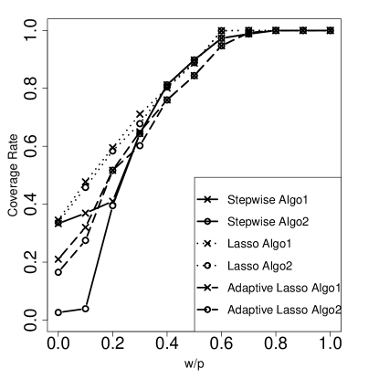
Figure 2: MUC of three model selection methods (Adaptive Lasso, Lasso, and stepwise regression using BIC) when applying to the diabetes data set. $B=1000$ bootstrap samples are generated from the original dataset. The tunning parameters of Adaptive Lasso and Lasso are chosen by 10-fold cross-validation. Two proposed algorithms are applied.

In Figure 2, we first compare the model selection methods using the MUC. As we can see, the coverage rate increases with the width $w$. The MUCs of all three methods arch towards the upper left corner. For Adaptive Lasso’s MUC, when $w=2$ and $w/p=0.2$, the coverage rate is around 0.4, meaning the MCB captures only about 40% of the bootstrap models. When $w>6$, the coverage rate stays above $0.9$, meaning that the MCB contains more than 90% bootstrap models. Recall that the interpretation of the MUC is similar to that of the more familiar ROC curve.

Table 1 further shows the 95%- and 75%-MCB of different model selection methods. When the confidence level increases, the LBM becomes smaller while the UBM becomes larger, and the cardinality of the MCB (i.e. number of unique models nested between LBM and UBM) also increases. Note that the bootstrap coverage rate is slightly larger than the confidence level due to the design of the algorithms. We also report the single selected models using these methods in the same table. As we can see, for each method, the 95%-MCB always contains the corresponding single selected model. According to our MCB results, the predictors bmi, ltg, map are considered most indispensable since they appear in most of the LBMs. Meanwhile, age is not included in any UBMs and should be excluded in the modeling process. Such a conclusion is also consistent with other existing studies (Lindsey and Sheather, 2010; Efron et al., 2004).

We also apply VSCS on this data set using the same confidence levels, 95% and 75%. The VSCS contains much more models than MCB (i.e., higher cardinality), suggesting that MCB can identify the true model more efficiently. For example, VSCS returns 528 and 288 unique models at confidence levels 95% and 75%, respectively. Compared these cardinalities with these of MCB (i.e., 16 and 64 for Adaptive Lasso, 16 and 32 for Lasso), we can see the clear advantage of MCB. Note that the models returned by MCB are always nested between the LBM and UBM, whereas the models returned by VSCS do not have such a structure, as they are simply the survivors of the F-test. Therefore, the models in VSCS are scattered in the entire space of all possible models (i.e., $2^{p}$ models). In addition, VSCS can be “roughly” considered as having multiple LBMs and having the full model as UBM since the full model by default will survive the F-test. However, note that VSCS does not contain all the models that are nested between its LBMs and UBM. Therefore, it is much harder to interpret VSCS results. We have summarized all LBMs and UBMs of VSCS in Table 1. At the confidence levels 95% and 75%, VSCS contains 7 and 4 different LBMs, respectively. They are all consistent with the LBM and UBM of MCB, in the sense that the predictors frequently appearing in LBMs of VSCS also appear in LBM of MCB. The predictors less frequently appearing in LBMs of VSCS are mostly in UBM of MCB.

5 Simulations

We investigate the performance of the proposed method by Monte Carlo (MC) experiments. Each MC sample is generated from the model, $y_{i}=\sum_{j=1}^{p^{\ast}}\theta_{j}x_{ij}+\sum_{j=p^{\ast}+1}^{p}0\times x_{ij}+\epsilon_{i}$, where $p^{\ast}$ is the number of true variables and $p$ is the number of candidate variables. We simulate the random error according to $\epsilon_{i}\sim N(0,\sigma^{2})$ and the covariate according to $\bm{x}_{i}\sim N_{p}(\bm{0},\bm{\Sigma})$ where $\bm{\Sigma}=[\Sigma_{ij}]_{p\times p}$ and $\Sigma_{ij}=\rho^{|i-j|}$. Additional simulations are in Web Appendix A.

Note that our simulation setting with the power decay correlation matrix $\bm{\Sigma}$ satisfies the Strong Irrepresentable Condition as proved by Corollary 3 in Zhao and Yu (2006), which provides the selection consistency of Lasso estimate. Other model selection methods used in this section include Adaptive Lasso, SCAD, MCP, LAD Lasso (Wang et al., 2007), and SQRT Lasso (Belloni et al., 2011), which are all proved to hold the property of selection consistency. Therefore, Assumption A.1 is satisfied. In addition, the modified residual bootstrap is used for Lasso estimate. The residual bootstrap is used for Adaptive Lasso, SCAD, MCP, LAD Lasso, and SQRT Lasso. These bootstrap algorithms provide valid approximations to the sampling distributions of the estimates and further guarantee Assumption A.2.

5.1 Comparison of Algorithms

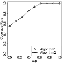
(a) $p=8$

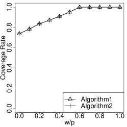
(b) $p=10$

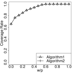
(c) $p=15$

(d) $p=50$

(e) $p=100$

(f) $p=200$

Figure 3: MUCs of Algorithms 1 and 2 for different scenarios with independent covariates. The top row shows the results of Algorithms 1 and 2: (a) $p=8$, $p^{*}=3$; (b) $p=10$, $p^{*}=4$; (c) $p=15$, $p^{*}=6$. The second row shows only Algorithm 2 because Algorithm 1 is infeasible in these cases: (d) $p=50$, $p^{*}=8$; (e) $p=100$, $p^{*}=10$; (f) $p=200$, $p^{*}=12$. The Adaptive Lasso is used as the variable selection method.

We consider six scenarios: (a) $p=8$, $p^{*}=3$; (b) $p=10$, $p^{*}=4$; (c) $p=15$, $p^{*}=6$; (d) $p=50$, $p^{*}=8$; (e) $p=100$, $p^{*}=10$; and (f) $p=200$, $p^{*}=12$. We set $n=300$, $B=1000$, $\theta_{j}=1$ and $\sigma=1$. In addition, we let $\rho=0$ and $0.5$ to simulate the cases of independent and correlated covariates. Adaptive Lasso with 10-fold cross-validation is used as the model selection method. Through simulation, we see that the MUCs from Algorithms 1 and 2 are very similar under these six scenarios using both independent and correlated covariates, indicating the performance (in terms of coverage) of Algorithms 1 and 2 are almost the same. For details of these MUCs, please see Figure 3 and Web Appendix A Figure LABEL:fig:illu_correlated. Note that Algorithm 1 uses the exhaustive search so its MUC is the highest possible and cannot be improved. Therefore, we conclude that Algorithm 2 performs (nearly) optimally as well. However, using Algorithm 1, MCB becomes impossible to obtain when $p$ is large because it requires too much time, while using Algorithm 2, we can easily obtain MCB. We further explore their computational times. To complete one MC iteration, Algorithm 1 takes 22.37, 207.64, 67750.81 seconds in scenarios (a), (b), and (c), and cannot compute at all for larger $p$s in scenarios (d), (e), and (f). On the other hand, Algorithm 2 takes less than 1 second in scenarios (a), (b), and (c), and 5.01, 22.70, 201.43 seconds in scenarios (d), (e), and (f). Such a phenomenon is not a surprise as explained in Section 3. Therefore, we adopt Algorithm 2 throughout the rest of the simulation studies.

5.2 Assessing Model Selection Uncertainty

One of the greatest advantages of MCB is to provide a platform to assess uncertainties of different model selection methods. We use the proposed method to demonstrate such an advantage under linear regressions.

We generate data according to the linear regression model and set $p^{*}=5$, $p=12$, $\theta_{j}=1$, $n=300$ and $B=1000$. We simulate the random error under two scenarios: $\epsilon_{i}\sim N(0,1)$ and $\epsilon_{i}\sim\textup{Laplace}(0,\sqrt{1/2})$, which give $\epsilon_{i}$ the same variance. In addition, we let $\rho=0$ and $0.5$ to simulate the cases of independent and correlated covariates. We compare various model selection methods with different loss functions and penalty functions. In particular, we include stepwise regression using BIC, Lasso, Adaptive Lasso, LAD Lasso, SQRT Lasso, SCAD and MCP. Note that Lasso, Adaptive Lasso, SCAD, and MCP have the same loss function, while Lasso, LAD Lasso, SQRT Lasso have the same penalty. Figure 4 shows the MUCs of different model selection methods under these simulation settings. Note that a more stable model selection method will have its MUC arch further towards the upper left corner. For the normal distribution, stepwise, Adaptive Lasso, SCAD and MCP perform better than the rest, because their loss function is compatible with the normal random errors. For the Laplace distribution, LAD Lasso and SQRT Lasso perform better than the rest, because LAD Lasso and SQRT Lasso are more robust against heavy tail random errors, therefore, offer lower model selection uncertainty. Such a phenomenon is consistent for both independent and correlated covariates. For numerical studies, stepwise regression is available in leaps, Lasso is available in glmnet, Adaptive Lasso is available in parcor, LAD Lasso and SQRT lasso are available in flare, and MCP and SCAD are available in ncvreg.

5.3 Comparison of MCB and VSCS

We further compare the performance of MCB with VSCS (Ferrari and Yang, 2015). Note that MCB is equipped with LBM and UBM and all the models contained in MCB are nested between LBM and UBM, whereas VSCS contains a basket of models which are the survivors of the F-test and hence are not necessarily nested. MCB is implemented by Adaptive Lasso while VSCS is implemented by F-test.

We simulate data according to the linear regression model with $n=100$, $B=1000$, $p^{*}=5$, $p=10$, $\theta_{j}=\gamma^{j}$ and $\sigma=1$. We set $\rho=0$, 0.25 and 0.5 to simulate the cases of independent and correlated covariates, and further set $\gamma=1$ and $0.6$ to simulate the constant coefficients and power decaying coefficients. Under these scenarios, we present the true model coverage rates of MCB and VSCS, cardinalities (i.e., the number of unique models returned by MCB and VSCS) in Table 2. As we can see, under the same confidence levels, both MCB and VSCS have approximately the same coverage rates, suggesting both of them are valid tools. MCB occasionally has higher coverage rates because of the design of the algorithm. On the other hand, MCB consists fewer models than VSCS and also preserves a structure of its model composition, which means MCB is more efficient in capturing the true model and its results are easier to interpret. Such a phenomenon persists even when we have correlated covariates and power decaying coefficients (i.e., $\rho=0.5$ and $\gamma=0.6$). However, using the power decaying coefficients, it is much harder to select the models. Therefore, the cardinality increases for both MCB and VSCS, but MCB still hold advantage over VSCS. The advantage of MCB over VSCS in these scenarios is partially due to the fact that VSCS does not incorporate an UBM (or equivalently, VSCS has the UBM of the full model since the full model always survives the F-test). On the other hand, MCB has both LBM and UBM, therefore, contains fewer models than VSCS. Lastly, VSCS uses F-tests to select models whereas MCB uses Adaptive Lasso, which also accounts for the advantage of MCB.

6 Conclusions

This paper introduces the concept of model confidence bounds (MCB) for variable selection and proposes an efficient algorithm to obtain MCB. Rather than blindly relying on a single selected model without knowing its credibility, MCB yields two bounds for models that capture a group of nested models which contains the true model at a given confidence level; it extends the notion of confidence interval for population parameter to the variable selection problem. MCB can be used as a model selection diagnostic tool as well as a platform for assessing different model selection methods’ uncertainty. By comparing the proposed MUC, we can evaluate the stabilities of model selection methods, just like we use confidence intervals to evaluate estimators. Therefore, MCB provide more insights into the existing variable selection methods and a deeper understanding of observed data sets.

There are many directions remaining for further research. For example, throughout this paper, we have assumed that MCB consists of one LBM and one UBM. However, it may be possible to find multiple LBMs that are statistically equivalent (Ferrari and Yang, 2015). Thus, we may consider a richer structure of MCB with multiple LBMs or even multiple UBMs. In addition, MCB can be extended to other classes models, such as, GLM and time series models (Meier et al., 2008; Zhou et al., 2015). We leave these topics for future research.

(a) Normal distribution, $\rho=0$

(b) Laplace distribution, $\rho=0$

(c) Normal distribution, $\rho=0.5$

(d) Laplace distribution, $\rho=0.5$

Figure 4: MUCs of different model selection methods for linear regression. The data generating model is $y=\sum_{j=1}^{5}1\times x_{j}+\sum_{j=6}^{12}0\times x_{j}+\epsilon$. Panel: (a) $\epsilon\sim N(0,1)$, (b) $\epsilon\sim\textup{Laplace}(0,\sqrt{1/2})$. $n=300$ and $B=1000$. Stepwise regression using BIC, Lasso, Adaptive Lasso, LAD Lasso, SQRT Lasso, SCAD and MCP are compared. Tuning parameters are chosen based on 10-fold cross-validation.

Method	$1-\alpha$	MCB	bmi	ltg	map	tc	sex	tch	ldl	glu	hdl	age	Width	Cardinality	CR
MCB ALasso	$0.95$	UBM											6	64	0.975
		LBM
	$0.75$	UBM											4	16	0.811
		LBM
MCB Lasso	$0.95$	UBM											5	32	0.999
		LBM
	$0.75$	UBM											4	16	0.805
		LBM
MCB Stepwise	$0.95$	UBM											6	64	0.973
		LBM
	$0.75$	UBM											5	32	0.812
		LBM
ALasso													-	-	-
Lasso													-	-	-
Stepwise													-	-	-
		UBM
VSCS	$0.95$	LBM1											-	528	-
		LBM2
		LBM3
		LBM4
		LBM5
		LBM6
		LBM7
		UBM
VSCS	0.75	LBM1											-	288	-
		LBM2
		LBM3
		LBM4

Table 1: Results of MCB with different variable selection methods (Adaptive Lasso, Lasso, and stepwise regression using BIC) and VSCS at 75% and 95% confidence levels. Light and dark gray cells denote that the predictors are in the LBM or UBM. $B=1000$ bootstrap samples are generated. Medium gray cells in the middle three rows denote that the predictors are selected in the single model after applying these variable selection methods to the original dataset. The bottom rows indicate the results of VSCS. Note that VSCS has multiple LBM at each confidence level and does not have UBMs. In addition, VSCS does not have width or CR.

			MCB		VSCS
$\rho$	$\gamma$	$100(1-\alpha)\%$	Coverage Rate	Cardinality	Coverage Rate	Cardinality
0	1	95%	0.93	31.65	0.94	32.57
0	1	90%	0.89	10.09	0.88	29.69
0	1	85%	0.87	5.51	0.82	27.58
0	1	80%	0.85	3.99	0.77	25.74
0	1	75%	0.83	3.14	0.72	23.91
0	1	70%	0.79	2.60	0.67	22.25
0	1	65%	0.76	2.27	0.62	20.53
0	1	60%	0.74	1.98	0.57	18.95
0.25	1	95%	0.96	8.02	0.96	36.36
0.25	1	90%	0.93	4.13	0.92	31.96
0.25	1	85%	0.90	3.06	0.85	29.17
0.25	1	80%	0.88	2.58	0.79	27.01
0.25	1	75%	0.86	2.20	0.76	25.15
0.25	1	70%	0.82	1.94	0.71	23.38
0.25	1	65%	0.80	1.73	0.68	21.65
0.25	1	60%	0.77	1.60	0.62	19.94
0.5	1	95%	0.92	8.25	0.95	49.74
0.5	1	90%	0.88	4.42	0.89	39.95
0.5	1	85%	0.84	3.21	0.85	34.60
0.5	1	80%	0.81	2.64	0.80	30.85
0.5	1	75%	0.80	2.33	0.76	28.11
0.5	1	70%	0.77	2.02	0.71	25.56
0.5	1	65%	0.74	1.80	0.66	23.42
0.5	1	60%	0.73	1.63	0.62	21.34
0	0.6	95%	0.98	266.20	0.94	291.80
0	0.6	90%	0.95	218.20	0.91	237.50
0	0.6	85%	0.93	190.70	0.84	203.50
0	0.6	80%	0.85	162.90	0.81	176.60
0	0.6	75%	0.77	140.50	0.75	155.60
0	0.6	70%	0.71	121.00	0.70	137.00
0	0.6	65%	0.69	113.30	0.64	121.10
0	0.6	60%	0.64	90.20	0.61	106.00
0.5	0.6	95%	0.94	279.00	0.92	320.20
0.5	0.6	90%	0.90	214.40	0.87	262.50
0.5	0.6	85%	0.84	176.60	0.84	227.30
0.5	0.6	80%	0.81	156.80	0.82	201.60
0.5	0.6	75%	0.73	132.50	0.79	179.60
0.5	0.6	70%	0.67	115.50	0.71	160.80
0.5	0.6	65%	0.61	99.80	0.66	143.50
0.5	0.6	60%	0.51	88.00	0.60	127.90

Table 2: Comparison of MCB and VSCS in terms of cardinalities and coverage rates at various confidence levels using both independent and correlated covariates and constant and exponentially decaying coefficients.

References

- Belloni et al. (2011) Belloni, A., Chernozhukov, V., and Wang, L. (2011). Square-root lasso: pivotal recovery of sparse signals via conic programming. Biometrika 98, 791–806.
- Camponovo (2015) Camponovo, L. (2015). On the validity of the pairs bootstrap for lasso estimators. Biometrika 102, 981–987.
- Chatterjee and Lahiri (2010) Chatterjee, A. and Lahiri, S. N. (2010). Asymptotic properties of the residual bootstrap for lasso estimators. Proceedings of the American Mathematical Society 138, 4497–4509.
- Chatterjee and Lahiri (2011) Chatterjee, A. and Lahiri, S. N. (2011). Bootstrapping lasso estimators. Journal of the American Statistical Association 106, 608–625.
- Chatterjee and Lahiri (2013) Chatterjee, A. and Lahiri, S. N. (2013). Rates of convergence of the adaptive lasso estimators to the oracle distribution and higher order refinements by the bootstrap. Annals of Statistics 41, 1232–1259.
- Efron et al. (2004) Efron, B., Hastie, T., Johnstone, I., and Tibshirani, R. (2004). Least angle regression. Annals of statistics 32, 407–499.
- Fan and Li (2001) Fan, J. and Li, R. (2001). Variable selection via nonconcave penalized likelihood and its oracle properties. Journal of the American Statistical Association 96, 1348–1360.
- Fan and Lv (2010) Fan, J. and Lv, J. (2010). A selective overview of variable selection in high dimensional feature space. Statistica Sinica 20, 101–148.
- Ferrari and Yang (2015) Ferrari, D. and Yang, Y. (2015). Confidence sets for model selection by F-testing. Statistica Sinica 25, 1637–1658.
- Freedman (1981) Freedman, D. A. (1981). Bootstrapping regression models. Annals of Statistics 9, 1218–1228.
- Hansen et al. (2003) Hansen, P. R., Lunde, A., and Nason, J. M. (2003). Choosing the best volatility models: The model confidence set approach. Oxford Bulletin of Economics and Statistics 65, 839–861.
- Hansen et al. (2005) Hansen, P. R., Lunde, A., and Nason, J. M. (2005). Model confidence sets for forecasting models. Technical report, Working Paper, Federal Reserve Bank of Atlanta.
- Hansen et al. (2011) Hansen, P. R., Lunde, A., and Nason, J. M. (2011). The model confidence set. Econometrica 79, 453–497.
- Leeb and Pötscher (2006) Leeb, H. and Pötscher, B. M. (2006). Can one estimate the conditional distribution of post-model-selection estimators? Annals of Statistics 34, 2554–2591.
- Lindsey and Sheather (2010) Lindsey, C. and Sheather, S. (2010). Variable selection in linear regression. Stata Journal 10, 650.
- Liu and Yu (2013) Liu, H. and Yu, B. (2013). Asymptotic properties of lasso+mls and lasso+ridge in sparse high-dimensional linear regression. Electronic Journal of Statistics 7, 3124–3169.
- Meier et al. (2008) Meier, L., Van De Geer, S., and Bühlmann, P. (2008). The group lasso for logistic regression. Journal of the Royal Statistical Society: Series B (Statistical Methodology) 70, 53–71.
- Pötscher and Schneider (2010) Pötscher, B. M. and Schneider, U. (2010). Confidence sets based on penalized maximum likelihood estimators in gaussian regression. Electronic Journal of Statistics 4, 334–360.
- Samuels and Sekkel (2013) Samuels, J. D. and Sekkel, R. M. (2013). Forecasting with many models: Model confidence sets and forecast combination. Technical report, Bank of Canada Working Paper.
- Shimodaira (1998) Shimodaira, H. (1998). An application of multiple comparison techniques to model selection. Annals of the Institute of Statistical Mathematics 50, 1–13.
- Tibshirani (1996) Tibshirani, R. (1996). Regression shrinkage and selection via the lasso. Journal of the Royal Statistical Society: Series B (Statistical Methodology) 58, 267–288.
- Wang et al. (2007) Wang, H., Li, G., and Jiang, G. (2007). Robust regression shrinkage and consistent variable selection through the LAD-Lasso. Journal of Business & Economic Statistics 25, 347–355.
- Zhang (2010) Zhang, C.-H. (2010). Nearly unbiased variable selection under minimax concave penalty. Annals of Statistics 38, 894–942.
- Zhao and Yu (2006) Zhao, P. and Yu, B. (2006). On model selection consistency of lasso. Journal of Machine Learning Research 7, 2541–2563.
- Zhou et al. (2015) Zhou, N., Cheng, W., Qin, Y., and Yin, Z. (2015). Evolution of high frequency systematic trading: A performance-driven gradient boosting model. Quantitative Finance 15, 1387 – 1403.
- Zou (2006) Zou, H. (2006). The adaptive lasso and its oracle properties. Journal of the American Statistical Association 101, 1418–1429.