CNO behaviour in planet-harbouring stars

Abstract

Context. Carbon, oxygen and nitrogen (CNO) are key elements in stellar formation and evolution, and their abundances should also have a significant impact on planetary formation and evolution.

Aims. We aim to present a detailed spectroscopic analysis of 1110 solar-type stars, 143 of which are known to have planetary companions. We have determined the carbon abundances of these stars and investigate a possible connection between C and the presence of planetary companions.

Methods. We used the HARPS spectrograph to obtain high-resolution optical spectra of our targets. Spectral synthesis of the CH band at 4300Å was performed with the spectral synthesis codes MOOG and FITTING.

Results. We have studied carbon in several reliable spectral windows and have obtained abundances and distributions that show that planet host stars are carbon rich when compared to single stars, a signature caused by the known metal-rich nature of stars with planets. We find no different behaviour when separating the stars by the mass of the planetary companion

Conclusions. We conclude that reliable carbon abundances can be derived for solar-type stars from the CH band at 4300Å. We confirm two different slope trends for [C/Fe] with [Fe/H] because the behaviour is opposite for stars above and below solar values. We observe a flat distribution of the [C/Fe] ratio for all planetary masses, a finding that apparently excludes any clear connection between the [C/Fe] abundance ratio and planetary mass.

1 Introduction

Carbon, together with nitrogen and oxygen, is one of the most abundant elements, after H and He. These elements play an important role in the lifetime of solar-type stars as they generate energy through the CNO cycle (Liang et al. 2001)

Carbon is created through a different process from nitrogen and oxygen. In this case, $\alpha$-chain reactions are the dominant processes. Both massive (M_⋆ ¿ 8$M_{\odot}$) and low- to intermediate-mass stars contribute to carbon production, but the relative importance of each type of star has not been clarified owing to uncertainties in the metallicity-dependent mass loss (see Meynet & Maeder 2002; van den Hoek & Groenewegen 1997)

It has been well-established that stars hosting a giant planet are, on average, more metal-rich than stars with no detected companion (Santos et al. 2001, 2004; Fischer & Valenti 2005; Gonzalez 2006; Buchhave et al. 2012). Two hypotheses have been proposed in an attempt to explain the nature of these metal-rich stars: The first one is self-enrichment, where the host star is polluted by planetesimals accreting on to the star. (see Israelian et al. 2001; Israelian et al. 2003) This self-enrichment scenario could lead to a relative overabundance of refractories, such as Si, Mg, Ca, Ti, and the iron-group elements, compared to volatiles, such as C, N, O, S, and Zn (Gonzalez 1997; Smith et al. 2001). The second one is the existence of a primordial cloud. Santos et al. (2001, 2002, 2003) found evidence that this over-abundance most is probably caused by a metal-rich primordial cloud.

The analysis of the HARPS stellar sample by Adibekyan et al. (2012b) shows that this chemical overabundance found in stars with planets is not exclusive to iron. Using a sample of 1111 FGK stars, they show that stars hosting a giant planet in their systems show an over-abundance in 12 refractory elements. They find that, at metallicities below $-$0.3 dex, about 76% of the planet hosts are enhanced in $\alpha$ elements at a given metallicity. This proves that planet formation requires a certain amount of metals, even for low-mass planets (Adibekyan et al. 2012c).

There are several studies of carbon in solar-type stars, but hardly any of these use CH molecular features (see Clegg et al. 1981). Instead, the most commonly used features are the $C_{2}$ Swan ($\lambda$ 5128 and $\lambda$5165), the CN molecular band ($\lambda$4215), and two atomic lines ($\lambda$ 5380.3 and $\lambda$5052.2). This last feature becomes very weak for cool stars ($\rm T_{\rm eff}$ ¡ 5100K).

Previous studies by Delgado Mena et al. (2010) and da Silva et al. (2011); Da Silva et al. (2015) using some of the above-mentioned carbon features show that there is no difference in behaviour regarding carbon between stars with and without any known planetary companion. The enrichment found was attributed to Galactic chemical evolution.

In this article we study the volatile C element using the CH band and derive C abundances for 1110 HARPS FGK stars, thereby complementing the Adibekyan et al. (2012b) study of refractory elements. We propose that CH molecular features are a good alternative to atomic lines. We also investigate whether the presence of a (giant) planetary companion affects the carbon abundance of the planet host stars.

2 Sample description

The high-resolution spectra analysed in this work were obtained with the HARPS spectrograph at La Silla Observatory (ESO, Chile) during the HARPS GTO programme (see Mayor et al. 2003; Lo Curto et al. 2010; Santos et al. 2011, for more information about the programme). The spectra had already been used in the analysis of stellar parameters, as well as the derivation of precise chemical abundances (see e.g. Sousa et al. 2008, 2011a, 2011b; Tsantaki et al. 2013; Adibekyan et al. 2012b).

The high spectral resolving power ($R=110,000$) of HARPS and a good signal-to-noise ratio (S/N) are an optimal combination for properly analysing the CH band at 4300Å. About 41$\%$ of the stars within our sample, at 4300Å, have S/N¿150, 18$\%$ have S/N in the range 100–150, and 30$\%$ have S/N below 100. Only 4$\%$ of our sample have S/N lower than 40.

The sample consists of 1110 FGK solar-type stars with effective temperatures between 4400 K and 7212 K, metallicities from $-1.39$ to $0.55$ dex, and surface gravities from $3.59$ to $4.96$ dex. 143 out of 1110 are planet hosts, whereas the other 967 are comparison sample or comparison stars (stars with no known planetary companion).

3 Analysis

3.1 Stellar parameters and chemical abundances

The stellar parameters used in this study were taken from Sousa et al. (2008, 2011a, 2011b) and Tsantaki et al. (2013), who used the same spectra as we did for this study. All the stellar parameters were derived by measuring equivalent widths of FeI and FeII lines using the ARES and ARES2 code (Sousa et al. 2007, 2015b). Chemical abundances of elements with spectral lines present in the features studied were obtained from Adibekyan et al. (2012b). These elements are Ca, Si, Sc, and Ti. Also, chemical abundances of elements other than carbon were adapted in targets with more recent stellar parameters (also obtained by our group using the aforementioned technique, see Tsantaki et al. 2013) following uncertainties presented in their original sources, so systematic effects in the chemical abundances or the stellar parameters are negligible and do not affect the consistency of our results.

Carbon abundances were determined using a standard local thermodynamic equilibrium (LTE) analysis with the MOOG spectral synthesis code (Sneden 1973, 2013 version) and a grid of Kurucz (1993) ATLAS9 atmospheres. All atmospheric parameters, $T_{\rm eff}$, $\log g$, $\xi_{t}$, and [Fe/H] were taken, as mentioned above, from Sousa et al. (2008, 2011a, 2011b) and Tsantaki et al. (2013). Adopted solar abundances for carbon and iron were $\log\epsilon(\rm C)_{\odot}=8.50$ dex and $\log\epsilon(\rm Fe)_{\odot}=7.52$ (Caffau et al. 2010; Caffau et al. 2011). For oxygen, we adopt $\log\epsilon(\rm O)_{\odot}=8.71$ dex (Bertran de Lis et al. 2015).

As molecular carbon abundances are affected by molecular equilibrium, we need to consider oxygen and nitrogen. Oxygen, being an $\alpha$-element, does not keep pace with [Fe/H] as nitrogen does (see Bertran de Lis et al. 2015; Suárez-Andrés et al. 2016). However, there were 575 stars with no previous measurements of O and 1054 stars with no previous measurements of N. We decided to use the available oxygen $\lambda 6158$ results and perform an interpolation for these 575 stars with no oxygen measurements (see Section 4.1). We obtained individual O and N abundances for the available targets from Bertran de Lis et al. (2015) and Suárez-Andrés et al. (2016), respectively. As nitrogen re-scales with [Fe/H], we obtained carbon abundances, thus providing individual values of oxygen and scaling nitrogen with the metallicity.

We did not consider NLTE effects because these features are likely to be immune to such effects at these metallicities, although little computational work has been done in this area (Asplund 2005; Schuler et al. 2008).

3.2 CH band

The CH band is the strongest feature observed in the spectral region $\lambda 4300\AA.$ We determined carbon abundances by fitting synthetic spectra to data in this wavelength range. The dissociation potential used for CH spectra is $D_{o}=3.464$ eV, as recommended in Grevesse et al. (1990). The complete line list used in this work was obtained from VALD3 (Ryabchikova et al. 2015). We slightly modified the log $gf$ values of the strongest lines in order to fit the solar spectrum.

The continuum was normalised locally with a fifth-degree polynomial, using the CONTINUUM task of IRAF.

To find the best fit abundance value for each star, we used the FITTING program (González Hernández et al. 2011) and the MOOG synthesis code in its 2013 version. The best fit was obtained using a $\chi^{2}$ minimization procedure, by comparing each synthetic spectrum with the observed one in the following spectral regions: $\lambda\lambda 4276.8-4282.2\AA$, $\lambda\lambda 4292.8-4293.4\AA$, $\lambda\lambda 4294.5-4298.3\AA$, $\lambda\lambda 4301.5-4303.7\AA$, $\lambda\lambda 4307.1-4310.7\AA$, $\lambda\lambda 4322.6-4324.6\AA$, $\lambda\lambda 4360.1-4360.6\AA$, $\lambda\lambda 4362.3-4367.0\AA$, $\lambda\lambda 4377.0-4377.4\AA$, and $\lambda\lambda 4387.2-4387.7\AA$. These regions were chosen for the presence of relatively strong CH features that allow reliable abundance measurements. We used a $\chi^{2}$ comparison between observed and synthetic spectra, and we define $\chi^{2}$=$\sum_{i=1}^{N}(F_{i}-S_{i})^{2}/N$, where $F_{i}$ and $S_{i}$ are the observed and synthetic fluxes, respectively, at wavelength point $i$. Best-fit carbon abundances were extracted from every spectral range and then the final carbon abundance for each star was computed as the average of these values. All the atmospheric parameters, $\rm T_{\rm eff}$, $logg$, $\xi_{t}$, [Fe/H] as well as all the chemical abundances used in the determination of C (see Section 3.1 and 4.1), were fixed. Rotational broadening was set as a free parameter with $v$ sin$i$ varying between 0.0 and 14.0 $km/s$ with a step of 1 km/s. For more information about the procedure followed, see Suárez-Andrés et al. (2016).

In Fig. 1 we show the observed and synthetic spectra for the Sun and two stars that are depicted for different temperature and metallicity within our sample. For these two stars, the best fit and two different carbon abundances are also shown.

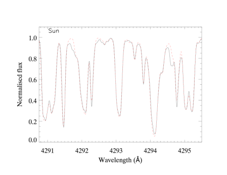
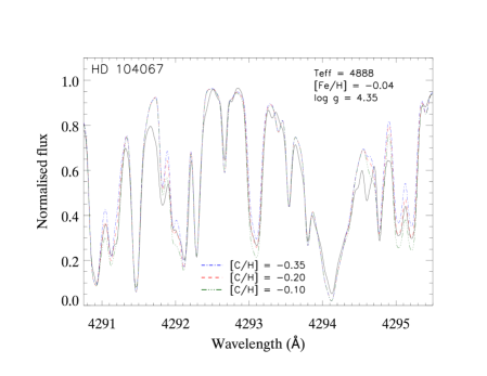
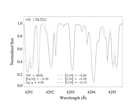
Figure 1: Top panel: observed solar spectrum (solid) and synthetic spectra (red-dashed lined). Middle and bottom panel: observed (solid) and synthetic spectra (green-dotted lined, red-dashed, and blue-dashed dotted) of HD 104067 and HD 136352.

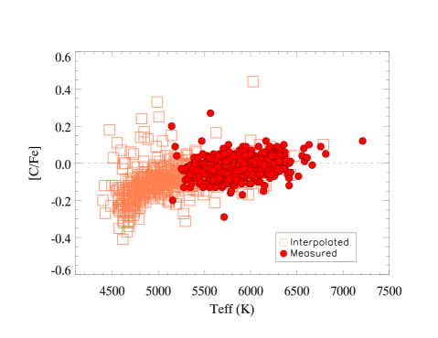
Figure 2: [C/Fe] as a function of $\rm T_{\rm eff}$. Filled red circles indicate those stars with available oxygen information, and open red squares indicate those stars with interpolated oxygen values.

To examine how variations in the atmospheric parameters affect carbon abundances, we tested the [C/H] sensitivity in stars with widely differing parameters, given the wide range of stellar parameters in our sample. For each set of stars, we tested the carbon abundance to changes in the stellar parameters ($\pm$50 K for $T_{\rm eff}$ and $\pm$0.1 dex in $\log g$ and metallicity). Results are shown in Table 3. The effect of microturbulence was not taken into account because an increase of 0.1 km s^-1 produced an average decrease of 0.0005 dex in carbon abundances, which is negligible with regard to the effects of other parameters. An error due to a continuum placement was considered for all stars of 0.05 in those stars with higher S/N and 0.1 for those with lower S/N, thereby increasing the considered continuum error with decreasing S/N. All effects were added quadratically to obtain the final uncertainties in carbon abundances following the expression:

$\Delta{\rm[C/H]}=(\Delta_{\sigma}^{2}+\Delta_{T_{\rm eff}}^{2}+\Delta_{\log g}^{2}+\Delta_{\rm[Fe/H]}^{2}+\Delta_{\rm cont}^{2}+\Delta_{\rm interp}^{2})^{1/2}$,

where $\Delta_{\sigma}$ refers to the error due to the $\chi^{2}$-fitting. The term $\Delta_{\rm interp}^{2}$ is added only for those stars with interpolated oxygen values.

4 Results

4.1 Carbon abundances

In 2015, Bertrán de Lis et al. (using the same spectra as in this work) obtained oxygen abundances for 698 stars by studying two atomic features: $\lambda 6158$ and $\lambda 6300$. We do not use $\lambda 6300$ results, because of the uncertainties of that feature caused by the presence of a blended nickel line. In order to obtain oxygen values for all our sample, we performed an interpolation of their [O/Fe] vs [Fe/H] results only for the $\lambda 6158$ feature. The interpolation consist of a 3^rd degree polynomial ($ax^{3}+bx^{2}+cx+d)$, where the coefficients are: $a=0.33$,$b=0.75$, $c=-0.36$, $d=0.03$). All the interpolations are consistent with an [O/H] vs [Fe/H] plot with previous measurements (González Hernández et al. 2013). We obtained oxygen abundances for 575 stars in order to complete the sample of 1110 stars.

In Fig. 2 we see carbon abundances as a function of $T_{\rm eff}$. We can see that for $T_{\rm eff}>4800$ K, both sets of data, those using real data and those using interpolated data, follow the same increasing trend for $T_{\rm eff}$ with similar dispersion (all stars from 4400 K to 5144 K have interpolated oxygen data). For those stars with $T_{\rm eff}<4800$ K we find a steep decrease in [C/Fe] abundance ratios with temperature. A similar effect can also be found for other $\alpha$-elements (Adibekyan et al. 2012b), as well as for nitrogen (Suárez-Andrés et al. 2016).

Stars with effective temperatures below 4800 K were excluded from the analysis because of uncertainties in the behaviour of those cool stars: we find no explanation for the decrease in carbon abundance as we move to lower temperatures.

4.2 Comparison with the literature

A few studies can be found that use the CH band at 4300Å, as opposed to C atomic lines. Delgado Mena et al. (2010) studied, among other elements, the carbon abundances of 451 stars of the HARPS sample, using the same spectra that we did. They used two atomic lines: $\lambda 5380.3$ and $\lambda 5052.2$. To confirm the validity of our study, we will compare our results of stars in common. In Fig. 3, top panel, we can see the molecular [C/H] results of these stars as a function of atomic [C/H]. Representing the 1:1 relation with a dashed line, we can see how the results show good agreement between themselves for effective temperatures above 5200 K, whereas for cooler stars the results show some disagreements. Thus, we have decided to continue only with the analysis of stars with effective temperatures above 5200 K.

In the bottom panel of Fig. 3 we show two sets: stars with $\rm T_{\rm eff}$¿5200 in common with Delgado Mena et al. (2010) (filled circle) and stars with $\rm T_{\rm eff}$¿5200 in common with Nissen et al. (2014) (open squares). Carbon abundances from Nissen et al. (2014) were obtained by studying the same atomic lines as in Delgado Mena et al. (2010). The slope of the fit, with its standard deviation, is provided for each set. As can be seen in Fig. 3, bottom panel, all sets (data from this work, Delgado Mena et al. (2010) and Nissen et al. (2014)) show good agreement

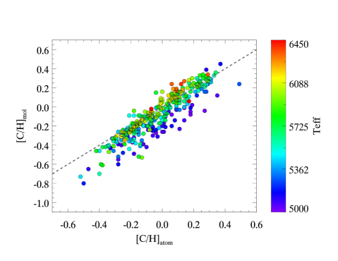
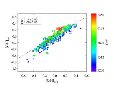
Figure 3: Top panel: molecular [C/H] results from this work as a function of atomic [C/H] extracted from Delgado Mena et al. (2010). The dashed line represents a 1:1 relation. Bottom panel: comparison for common stars with the works of Delgado Mena et al. (2010) (filled circles) and Nissen et al. (2014) (open squares) for stars with $\rm T_{\rm eff}$¿5200K.

5 Carbon abundances in stars with and without planets

We analysed optical high-resolution spectra of 112 planet host stars and 639 comparison stars. We aim to explore possible differences in carbon abundances between both samples. Our results can be found in an online table, along with the stellar parameters. A sample listing is shown in Table 1.

Table 1: Sample of carbon abundances for a set of stars with and without planets (see online table).

Star	$\rm T_{\rm eff}$	$logg$	$\xi_{t}$	[Fe/H]	[C/H]	Planet?	Pop.
	(K)	(cm $s^{-2})$	$(kms^{-1})$
HD 114386	4774	4.37	0.01	-0.09	-0.11 $\pm$ 0.11	Y	Thin
HD 104067	4888	4.35	0.66	-0.04	-0.16 $\pm$ 0.09	Y	Thin
HD 169830	6370	4.20	1.56	0.18	0.24 $\pm$ 0.08	Y	Thin
HD 136352	5659	4.40	0.90	-0.35	-0.35 $\pm$ 0.07	Y	Thick
BD+063077	6136	4.95	1.07	-0.36	-0.33 $\pm$ 0.15	N	Thick
HD 215902	5454	4.46	0.53	-0.25	-0.32 $\pm$ 0.12	N	Thin
HD 125522	4839	4.45	0.40	-0.46	-0.45 $\pm$ 0.12	N	Thin
HD 129229	5872	3.89	1.37	-0.42	-0.42 $\pm$ 0.09	N	Thin
…

To test for a possible relation between carbon abundances and the masses of planetary companions, we separated the planet population into two groups: low-mass planets (LMP; with masses less than or equal to 30 $M_{\oplus}$) and high-mass planets (HMP; with masses greater than 30 $M_{\oplus}$). In those stars which host several planets, the most massive planet was considered in our study. Our sample consists of 23 low-mass and 89 high-mass planet hosts.

We also look for distinguishable trends between these samples by representing [C/Fe] as a function of $T_{\rm eff}$ (see Fig. 4). As mentioned, we find a increasing trend of the [C/Fe] abundances on $T_{\rm eff}$ (for both planet and non-planet-hosts). However, the spread of [C/Fe] abundance values with $T_{\rm eff}$ amounts to about 0.1 dex from 5200 K to 6200 K, with $\sim$65% of our sample with [C/Fe] ¡ 0.0. Statistics for these relations are provided in Table 2. In Fig. 4 we can see the line at 4800 and 5200 K separating the cool stars from the sample studied.

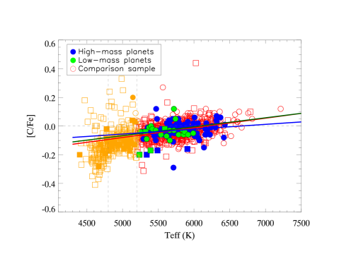
Figure 4: [C/Fe] vs. $T_{\rm eff}$. Filled circles represent planet hosts and open circles, the comparison sample. Squares represent interpolated oxygen values.

We looked for distinguishable trends between the host and non-planet host samples by representing [C/Fe] and [C/H] abundance ratios as functions of [Fe/H] (see Fig. 5). In Fig. 5 top panel, [C/H] vs. [Fe/H] is represented. We can see how all the samples behave in the same way, and that no difference between them can be found. If we look at the slopes of each sample, we find very similar values, thus confirming that stars with and without planets follow the same trend.

In the bottom panel of Fig. 5, we find that [C/Fe] follows the same trend found in other $\alpha$-elements. As presented in Da Silva et al. (2015), a decreasing trend can be found for metallicity values below solar, whereas for super-solar values, this trend has a positive slope. We can see in Fig. 5 how the slope for planets and the comparison sample at high metallicities follows the same behaviour, whereas for the low iron abundances the planet-host trend is steeper than for the comparison sample (for comparison sample only those stars with [Fe/H] ¿ -0.74 are taken (the minimum metallicity found for a planet host star in our sample)). This behaviour is consistent for stars with both low- and high-mass planetary companions. Statistics for these relations are also provided in Table 2.

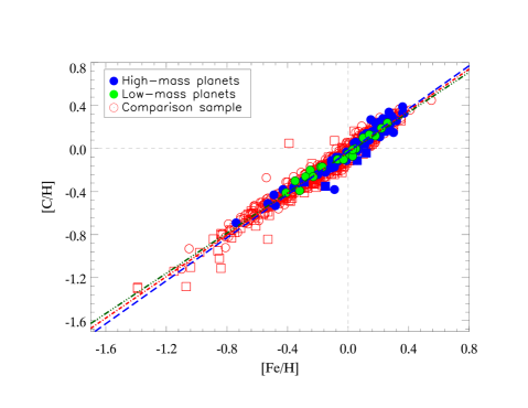
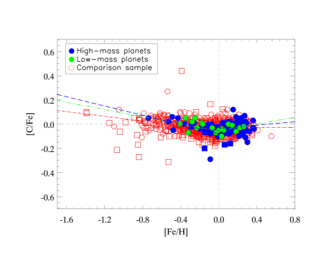
Figure 5: [C/H] and [C/Fe] vs. [Fe/H] plots. Filled circles represent planet hosts and the open circle, the comparison sample. Dotted lines represent solar values. Squares stand for interpolated oxygen values.

To evaluate the significance of the correlations we performed a simple bootstrapped Monte Carlo test. For more details on the test we refer the reader to Figueira et al. (2013) and Adibekyan et al. (2014).

Table 2: Statistics for the three groups studied (Comparison sample - NP, low-mass planets - LMP, high-mass planets - HMP) for [C/H] vs [Fe/H] and [C/Fe] vs Teff and [Fe/H] (see Figs. 4 and 5).

		[C/Fe] vs Teff
	Slope	Slopeerr	R	$\sigma_{R}$
NP	6.74E-05	7.13E-06	0.35	8.7
LMP	6.24E-05	3.95E-05	0.33	1.5
HMP	3.38E-05	2.16E-05	0.17	1.6
		[C/H] vs [Fe/H]
	Slope	Slopeerr	R	$\sigma_{R}$
NP	0.97	8.02E-03	0.98	24.5
LMP	0.93	4.06E-2	0.98	4.6
HMP	1.00	2.90E-02	0.97	9.0
		[C/Fe] vs [Fe/H]
		(for [Fe/H] ¡ 0.0)
	Slope	Slopeerr	R	$\sigma_{R}$
NP	-0.10	1.57E-02	-0.31	6.1
LMP	-0.15	8.24E-02	-0.46	1.7
HMP	-0.20	8.31E-02	-0.49	2.5
		[C/Fe] vs [Fe/H]
		(for [Fe/H] ¿ 0.0)
	Slope	Slopeerr	R	$\sigma_{R}$
NP	0.00	3.46E-02	0.01	0.1
LMP	0.14	1.10E-1	0.44	1.2
HMP	0.07	7.50E-02	0.12	0.9

Table 3: Sensitivity of the carbon abundance derived from the CH band at 4300Å. Changes of 50K in $T_{\rm eff}$, 0.1 dex in gravity and 0.1 in [Fe/H] were applied.

			Star
			($\rm T_{\rm eff}$; $logg$; [Fe/H])
	HD 103720	HD 222595	HD 75881	HD 66740
	(5017; 4.43; -0.02)	(5618; 4.43; -0.01)	(6239; 4.44; 0.07)	(6666; 4.49; 0.04)
$\Delta T_{\rm eff}=\pm$ 50K	$\pm 0.03$	$\pm 0.03$	$\pm 0.06$	$\pm 0.04$
	HD 159868	HD 168746	HD 290327	HD 41087
	(5552; 3.91; -0.09)	(5561; 4.31; -0.11)	(5505; 4.41; -0.14)	(5562; 4.52; -0.13)
$\Delta\rm logg$ = $\pm$ 0.1 dex	$\mp 0.02$	$\mp 0.01$	$\pm 0.00$	$\pm 0.00$
	HD 68089	HD 161098	HD 206163	HD 203384
	(5597; 4.53; -0.77)	(5574; 4.49; -0.26)	(5506; 4.42; 0.02)	(5564; 4.42; 0.26)
$\Delta\rm([Fe/H])=\pm$ 0.1 dex	$\mp 0.13$	$\mp 0.02$	$\mp 0.02$	$\mp 0.02$

Since the discovery of the first exoplanet around a main-sequence star back in 1995 (Mayor & Queloz 1995), the number of known exoplanets has increased exponentially. Such discoveries have been made for a wide diversity of stars. Many studies of the hosts stars have proved that the formation of high-mass planets correlates with the metal content of the star (see Santos et al. 2001, 2004; Fischer & Valenti 2005; Sousa et al. 2011a; Mortier et al. 2013; Buchhave et al. 2012). Moreover, it has been shown that the formation of planets at low metallicities is favoured by enhanced $\alpha$-elements (Adibekyan et al. 2012a, c).

In Fig. 6 we can see the relative frequency of the planetary samples compared with the comparison sample (NP). The reader should be aware that undetected low-mass planets might be present in the comparison sample. In the top panel we show the [C/Fe] distributions for all the samples and find no differences among them. In the middle panel, we show [C/H] distributions for the same samples. There is a slight offset between the samples, especially between the comparison and the high-mass planet sample. We can confirm that the high-mass planet offset found for [C/H] is due to the metal-rich nature of their host stars, as no carbon enhancement is found (see Fig. 5, bottom). We found a completely different behaviour for the low-mass planetary sample, which does not seem to be preferentially metal-rich (Ghezzi et al. (2010); Sousa et al. (2008); Mayor et al. (2011); Sousa et al. (2011b); Buchhave et al. (2012); Buchhave & Latham (2015)). In the bottom planel, we show [C/H] but for solar analogue (stars with ($T_{\rm eff}=T_{\rm eff,\odot}\pm 300$ K, but not neccesarily solar gravity or metallicity). Statistics for these results are provided in Table 4.

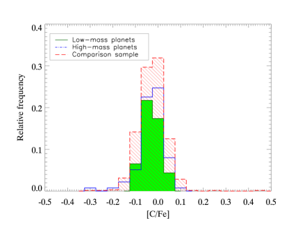
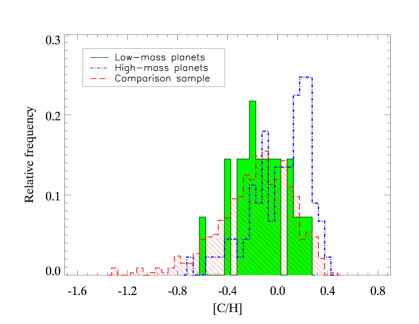
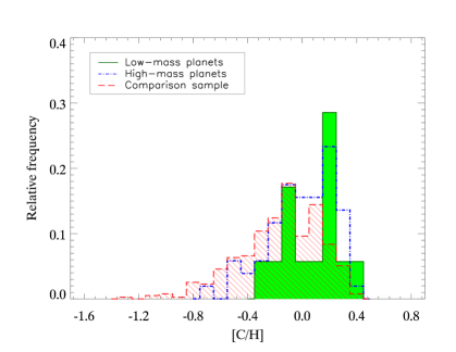
Figure 6: Top panel: [C/Fe] distributions of three different samples: stars without planets (NP, in red), low-mass planets (LMP, in green), and high-mass planets (HMP, in blue). Middle panel: [C/H] distributions for the three mentioned samples. Bottom panel: [C/H] distributions for the same three groups, but considering only solar analogues ($T_{\rm eff}=T_{\rm eff,\odot}\pm 300$ K)

Table 4: Statistics for the three samples studied (comparison sample - NP, low-mass planets - LMP, high-mass planets - HMP) for [C/H] and [C/Fe] abundances. Also, [C/H] abundances for those stars considered as solar analogues ($T_{\rm eff}=T_{\rm eff,\odot}\pm 300$ K) are provided.

			[C/Fe]
	Mean	SD	Median	Minimum	Maximum
NP	-0.03	0.06	-0.02	-0.31	0.44
LMP	-0.03	0.04	-0.03	-0.11	0.05
HMP	-0.03	0.06	-0.02	-0.29	0.12
			[C/H]
	Mean	SD	Median	Minimum	Maximum
NP	-0.17	0.29	-0.14	-1.30	0.45
LMP	-0.13	0.21	-0.17	-0.62	0.24
HMP	0.03	0.23	0.10	-0.69	0.39
			$\rm[C/H]_{analogs}$
	Mean	SD	Median	Minimum	Maximum
NP	-0.03	0.06	-0.02	-0.31	0.44
LMP	-0.03	0.04	-0.03	-0.11	0.05
HMP	-0.03	0.06	-0.02	-0.29	0.12

To see if there is any resemblance between each sub-sample of planet host with the non-planet host sample, we performed a Kuiper test (also known as invariant Kolmogorov–Smirnov (K–S) test), instead of the usual K–S test. Although K–S is suitable in our case, its sensitivity is higher around the median value, neglecting the tails. The Kuiper test compares two cumulative distribution functions and obtains the sum of the maximum distances above and below $S_{N}(x)$, where $S_{N}(x)$ is the cumulative distribution function of the probability distribution from which a dataset with $N$ events is drawn. In our study, a zero value of the K–S test refers to datasets with no similarities among them. Unity refers to the maximum similarity that can be found for the compared datasets (Press et al. 1992; Kirkman, T.W. 1996).

In Fig. 7 we can see the cumulative fraction for both [C/H] and [C/Fe] for the three cases: stars with high-mass planets (HMP) stars with low-mass planets (LMP), and the comparison sample (NP). In the top panel, we can see how all samples behave in a similar way. If we apply a Kuiper test to these samples, as shown in Table 5, we can see that all the samples share similarities: when taking [C/Fe] into account, the high-mass planetary sample behaves like the non-planet hosts and low-mass samples, as there is a probability of similarity between them. The planetary samples, however, separate from each other in [C/H]. Whereas the small-planet sample is more in agreement with the non-planet host sample, the high-mass planet sample detaches itself completely from this behaviour. These results are consistent with the results represented in Fig. 6.

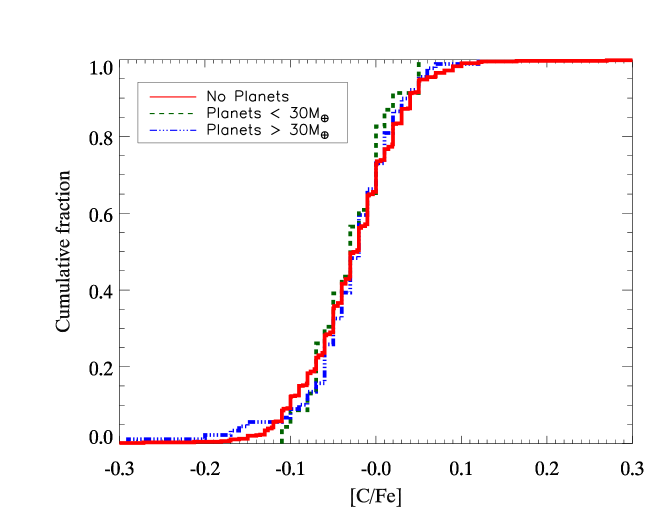
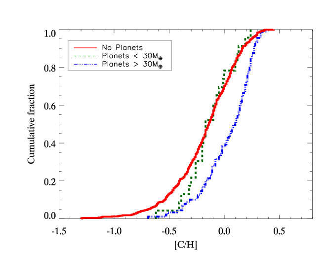
Figure 7: Top: Cumulative functions for the three different samples (LMP, HMP, and NP) for [C/H] abundances. Bottom: Cumulative functions for the three different samples (LMP - green, HMP - blue, and NP - red) for [C/Fe] abundances.

We looked deeper into the relation between [C/Fe] and the mass of the planet, as shown in the top panel of Fig. 8. The masses of the planets range between 0.0097 and 47 $M_{\rm J}$ (Only one star has a companion of 47 $M_{\rm J}$, which can be considered a brown dwarf, according to the standard definition of brown dwarf), but most stars have planets with less than 1 $M_{\rm J}$ orbiting around them. To remove this bias due to the lack of planets with higher masses, we created bins with increasing steps, with bin sizes of 0.03, 0.07, 0.2, 0.3, 0.4, 2.0, 3.0, 5.0, 10.0, and 27.0 $M_{\rm J}$. Error bars indicate the standard deviation of each bin. We can see how the [C/Fe] ratio shows a flat tendency for all masses because the deviation is negligible. We tested a possible relation between [C/Fe] and the planetary mass and obtained a covariance $s_{x,y}=0.001$, where $x=M_{\rm J}$ and $y=$ [C/Fe]. In the bottom panel of Fig. 8, we reduce the sample to solar analogues. In our case, we considered as solar analogues those stars with $T_{\rm eff}=T_{\rm eff,\odot}\pm 300$ K. We obtained a covariance $s_{x,y}=0.003$.

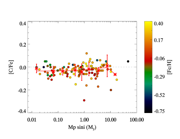
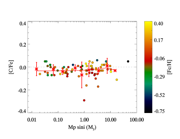
Figure 8: [C/Fe] versus $M_{\rm p}sini$ plot. Filled circles represent the whole sample, whereas red asterisks represent binned values. Hotter colours represent metallicities above solar while cooler colours represent metallicies below solar. Also in red, the fit for these binned values. In the top panel, for all the studied sample, in the bottom, for solar analogues ($T_{\rm eff}=T_{\rm eff,\odot}\pm 300$ K)

6 Kinematics properties and stellar populations

To study the kinematic properties of the sample stars and the stellar populations they belong to, we took the classification obtained by Adibekyan et al. (2012b), who applied both purely chemical (e.g. Adibekyan et al. 2011; Adibekyan et al. 2013; Recio-Blanco et al. 2014) and kinematic approaches (e.g. Bensby et al. 2003; Reddy et al. 2006) to classify their stars. The Galactic space velocity components of the stars were calculated in Adibekyan et al. (2012b) using the astrometric and radial velocity data of the stars. The average errors in the $U$, $V$, and $W$ velocities are about 2–3 km s^-1. The main source of the parallaxes and proper motions was the updated version of the Hipparcos catalogue (van Leeuwen 2007). Data for eight stars with unavailable Hipparcos information were taken from the TYCHO Reference Catalog (Hog et al. 1998).

The separation of the Galactic stellar components based only on stellar abundances is probably superior to that based on kinematics alone (e.g. Navarro et al. 2011; Adibekyan et al. 2011) because chemistry is a relatively more stable property of sunlike stars than their spatial positions and kinematics. We used the position of the stars in the [$\alpha$/Fe]–[Fe/H] plane (here $\alpha$ refers to the average abundance of Si, Mg, Ti) to separate the thin- and thick-disc stellar components. We recall that Ca was not included in the $\alpha$ index, because at super-solar metallicities the [Ca/Fe] trend differs from that of other $\alpha$-elements (Adibekyan et al. 2012b). We have adopted the boundary (separation line) between the stellar populations from Adibekyan et al. (2011). According to our separation, 640 stars ($\approx$85 per cent) are not enhanced in $\alpha$-elements and belong to the thin-disc population. The [$\alpha$/Fe] versus [Fe/H] plot for the sample stars is shown in the bottom panel of Figure 9.

In the top panel of Fig. 9 we show the dependence of [C/$\alpha$] on the metallicity. This trend is expected if the C abundance scales with the iron abundance, as was suggested above. It is interesting to note that at super-solar metallicities, [C/$\alpha$] remains almost constant for both samples.

Table 5: Kuiper test for the sample. We tested the relation between the low-mass planets (LMP) sample, the high-mass planets sample (HMP) and the comparison sample (NP) sample, for both [C/Fe] and [C/H]. Zero represents no similarity between the samples while unity represents the maximum similarity.

Sample	[C/Fe]	[C/H]
LMP - NP	0.54	0.72
HMP - NP	0.65	2.19e-08
LMP - HMP	0.85	3.78-03

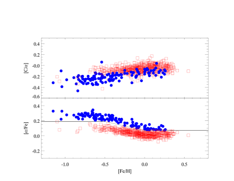
Figure 9: [C/$\alpha$] and [$\alpha$/Fe] vs. [Fe/H]. Stars that are enhanced in $\alpha$-elements are shown as blue squares and non-$\alpha$-enhanced stars are represented by red squares.

In Fig. 10 we present [C/Fe] against [Fe/H] for the sample of solar analogues. The selected stars have $T_{\rm eff}=T_{\rm eff,\odot}\pm 300$ K in the top panel and $T_{\rm eff}=T_{\rm eff,\odot}\pm 150$ K in the bottom panel. These solar analogues also have S/N ¿ 200 to ensure optimal accuracy in our conclusions.

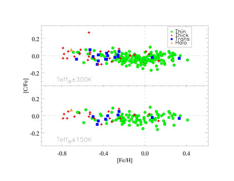
Figure 10: [C/Fe] versus [Fe/H] for solar analogues with S/N $\geq$ 200. Filled green dots refer to to the thin-disc population, filled blue squares to transition objects, orange triangles to halo stars, and red stars to thick-disc stars.

Figure 10 shows that, opposite to the chemical separation (using Ti, Mg, and Si for the $\alpha$ abundances), the thin and thick discs are not chemically different for C. In Adibekyan et al. (2012b), it was suggested that several $\alpha$-elements show different trends with metallicity.

7 Summary and conclusions

We present carbon abundances for 1110 solar-type stars observed with HARPS. In our sample, 143 of the 1110 are planet-hosts and 967 stars have no known planetary companion. All the targets have been studied using spectral synthesis of the CH band at 4300Å. All the stars within our sample have effective temperatures between 4400 K and 7212 K, metallicities from $-1.39$ to $0.55$ dex, and surface gravities from $3.59$ to $4.96$ dex.

We have performed a detailed spectral analysis of this sample to obtain precise carbon abundances and investigate possible differences between stars with planets and the comparison sample. We confirm that both samples, planet host stars and comparison stars, show no different behaviour when we study their carbon abundances as a function of different stellar parameters such as $T_{\rm eff}$ and [Fe/H].

We have compared our results with similar work (Delgado Mena et al. 2010), as seen in Fig 3. When comparing stars common to both works, we get agreement between the atomic and the molecular results, thus ensuring that molecular abundances from the CH 4300Å band can be a reliable alternative to atomic values.

We searched for a correlation between the presence of planets and carbon abundances. We found that both planet-hosts and non-planet-hosts usually have [C/Fe] $\leq$ 0.0 ($\sim$65% of the sample). We searched for a correlation between the carbon abundance and the planetary masses but found a flat trend for all the masses.

We looked for similarities between the three samples studied: the non-planet host samples and the low- and high-mass planetary sample. We found that both low- and high-mass planet hosts are not different from the comparison sample. None of the samples show signs of carbon enhancement.

We performed a chemical and kinematic separation for our sample and obtained a clear separation between the thin and the thick disc populations based on a dependence of [C/$\alpha$] with metallicity. However, no differences in carbon abundances can be found for the different stellar populations. We conclude that the molecular CH band located at 4300Å can be used to obtain reliable and accurate carbon abundances and therefore provide an accurate measurement of C/O ratios that can be used to investigate the mineralogy of exoplanets (Suárez-Andrés et al. 2016, in prep).