Weak lensing magnification in the Dark Energy Survey Science Verification data

Abstract

In this paper the effect of weak lensing magnification on galaxy number counts is studied by cross-correlating the positions of two galaxy samples, separated by redshift, using the Dark Energy Survey Science Verification dataset. This analysis is carried out for galaxies that are selected only by its photometric redshift. An extensive analysis of the systematic effects, using new methods based on simulations is performed, including a Monte Carlo sampling of the selection function of the survey.

1 Introduction

Weak gravitational lensing of distant objects by the nearby large-scale structure of the Universe is a powerful probe of cosmology (Bartelmann & Schneider, 2001; Meylan et al., 2006; Hoekstra & Jain, 2008; van Waerbeke et al., 2010; Weinberg et al., 2013; Kilbinger, 2015) with two main signatures: magnification and shear.

Magnification is due to the gravitational bending of the light emitted by distant sources by the matter located between those sources and the observer (Blandford et al., 1989). This leads to an isotropic observed size enlargement of the object while the surface brightness is conserved (Blandford & Narayan, 1992), modifying three observed properties of the sources: size, magnitude and spatial density. The change of spatial density of galaxies due to gravitational lensing is known as number count magnification and arises from the increase of the observed flux of the background galaxies, allowing the detection of objects that, in the absence of lensing, would be beyond the detection threshold (Bartelmann, 1992b). Magnification is dependent on the mass of the dark matter content along the line of sight to the source (Bartelmann, 1992a, c, 1995b; Bartelmann & Narayan, 1995). Therefore, its effect is not homogeneous and is spatially correlated with the location of lens galaxies and clusters, which are biased tracers of the dark matter field (White & Rees, 1978; Kaiser, 1984).

Since magnification and shear are complementary effects of the same physical phenomenon, they depend on the same cosmological parameters, but in a slightly different manner. Thus, some degeneracies are broken on parameter constraints (e.g. at the $\Omega_{M}-\sigma_{8}$ plane) when combining magnification with shear-shear correlations (van Waerbeke, 2010). Nevertheless, the major power of the combination of both methods is that they are sensitive to different sources of systematic errors. For example, number count magnification is independent of those systematic effects caused by shape determination, although it suffers from selection effects (Morrison & Hildebrandt, 2015). This constitutes a powerful feature that can be exploited to minimize systematic effects on a possible combination of magnification with galaxy-shear (gg-lensing) since both measurements are produced by the convergence field.

Extensive wide-field programs have allowed accurate measurements of weak lensing effects. Previous magnification measurements involve the use of very massive objects as lenses, such as luminous red galaxies (LRGs) and clusters (Broadhurst, 1995; Bauer et al., 2014; Ford et al., 2014; Chiu et al., 2016), or high redshift objects as sources, such as Lyman break galaxies (LBGs; Hildebrandt et al. (2009); Morrison et al. (2012)) quasars (Seldner & Peebles, 1979; Hogan et al., 1989; Fugmann, 1990; Bartelmann & Schneider, 1993; Ménard & Bartelmann, 2002; Gaztañaga, 2003; Scranton et al., 2005) and sub-mm sources (Wang et al., 2011) to improve signal-to-noise ratio. In addition to the number count technique used in this paper, other observational effects produced by magnification have been measured as well: the shift in magnitude (Ménard et al., 2010), flux (Jain & Lima, 2011) and size (Huff & Graves, 2014).

Lyman break galaxies and quasars have demonstrated to be a very effective population of background samples to do magnification studies due to its high lensing efficiency. However deep surveys or large areas are needed to reach a significant number of these objects. Thus, shallow or small area surveys require the selection of a more numerous population of source galaxies to allow the measurement of the magnification signal.

In this paper, the magnification signal is measured using the number-count technique on the Dark Energy Survey (DES) Science Verification data. All observed galaxies, selected only with photometric redshifts, are used both as lenses and sources. This procedure simplifies the analysis as no addition processing or selections are needed to construct the sample, as in the dropout technique used for LBG selection. This alternative way to select galaxies is different to what is found on previous works, and provides a more numerous source sample. This allows the detection of magnification on small area surveys –such as the DES Science Verification data–, but the main power of this methodology resides on photometric surveys with large areas such as LSST and the final footprint of DES, with 5000 deg². The increase on the density of sources on large areas provides a huge number of total sources, reducing dramatically the shot-noise.

In addition, this paper presents an extensive test for systematic effects. New techniques, based on simulations specially developed for this purpose are used, including a Monte Carlo sampling method to model the selection function of the survey.

The structure of the paper is as follows: in section 2 the theory behind magnification is summarized. The steps leading to a detection are described in section 3, and section 4 describes the data sample. The methodology is validated in section 5 with a study on N-body simulations. The analysis of the data sample is made in section 6, concluding in section 7.

2 Number Count Magnification

Number count magnification can be detected and quantified by the deviation of the expected object counts in the positional correlation of a foreground and a background galaxy sample (Seldner & Peebles, 1979). These galaxy samples, in absence of magnification, are uncorrelated if their redshift distributions have a negligible overlap. In this section, the formalism that will quantify its effect on this observable is presented.

The observed two-point angular cross-correlation function between the i- and j-th redshift bins, including magnification, is defined as (Bartelmann, 1995a)

$$\omega_{ij}(\theta)=\langle\delta_{O}(\boldsymbol{\hat{n}},z_{i},f_{i})\delta_{O}(\boldsymbol{\hat{n}^{\prime}},z_{j},f_{j})\rangle_{\theta},$$ (1)

where $\theta$ is the angle subtended by the two direction vectors $\boldsymbol{\hat{n}},\boldsymbol{\hat{n}^{\prime}}$ and the observed density contrast ($\delta_{O}$) is

$$\delta_{O}(\boldsymbol{\hat{n}},z_{i},f_{i})=\delta_{g}(\boldsymbol{\hat{n}},z_{i})+\delta_{\mu}(\boldsymbol{\hat{n}},z_{i},f_{i});$$ (2)

where $\delta_{g}$ describes the fluctuations due to the intrinsic matter clustering at redshift $z_{i}$ and $\delta_{\mu}$ incorporates the fluctuations from magnification effects at a flux cut $f_{i}$.

The galaxy density contrast in the linear bias approximation is (Peacock & Dodds (1994); Clerkin et al. (2015))

$$\delta_{g}(\boldsymbol{\hat{n}},z_{i})=b_{i}\delta_{M}(\boldsymbol{\hat{n}},z_{i})$$ (3)

with $b_{i}$ the galaxy-bias at redshift $z_{i}$ and $\delta_{M}$ the intrinsic matter density contrast.

Following the approach used by Bartelmann & Schneider (2001) and Ménard et al. (2003), the magnification density contrast on the sky in direction $\boldsymbol{\hat{n}}$ is defined as

$$\delta_{\mu}(\boldsymbol{\hat{n}},z,f_{\mu})=\frac{N_{\mu}(\boldsymbol{\hat{n}},z,f_{\mu})}{N_{0}(\boldsymbol{\hat{n}},z,f_{0})}-1.$$ (4)

Here $N_{0}(\boldsymbol{\hat{n}},z,f_{0})$ is the unlensed cumulative number count of sources located at redshift $z$, that is, the number of sources with observed flux greater than the threshold $f_{0}$, while, $N_{\mu}(\boldsymbol{\hat{n}},z,f_{\mu})$ is the lensed cumulative number count, affected by magnification.

Magnification by gravitational lenses increases the observed flux of background galaxies allowing one to see fainter sources changing the effective flux cut from $f_{0}$ to $f_{\mu}=f_{0}/\mu$. At the same time it stretches the solid angle behind the lenses, reducing the surface density of sources down to $N_{\mu}=N_{0}/\mu$ (Narayan, 1989). Thus the density contrast may be rewritten as

$$\delta_{\mu}(\boldsymbol{\hat{n}},z,f_{\mu})=\frac{N_{\mu}(\boldsymbol{\hat{n}},z,f_{\mu})}{\mu N_{\mu}(\boldsymbol{\hat{n}},z,\mu f_{\mu})}-1.$$ (5)

The cumulative number count can be locally parametrized as

$$N_{\mu}(\boldsymbol{\hat{n}},z,f_{\mu})=A\left(\frac{f_{\mu}}{f_{*}}\right)^{\alpha(f_{\mu})}$$ (6)

where $A,f_{*}$ are constant parameters and $\alpha(f_{\mu})$ is a function of the flux limit. Substituting this parametrization into Equation 5:

$$\delta_{\mu}(\boldsymbol{\hat{n}},z,f_{\mu})=\mu^{-\alpha(f_{\mu})-1}-1.$$ (7)

Taking the weak lensing approximation, $\mu\simeq 1+2\kappa$ with $\kappa\ll 1$, where $\kappa$ corresponds to the lensing convergence of the field (Bartelmann & Schneider, 1992), and converting from fluxes to magnitudes, the previous equation becomes (Narayan & Wallington, 1993)

$$\delta_{\mu}(\boldsymbol{\hat{n}},z,m)=2\kappa(\boldsymbol{\hat{n}},z)\left[\alpha(m)-1\right]$$ (8)

with

$$\alpha(m)=2.5\frac{d}{dm}[\log N_{\mu}(m)].$$ (9)

The convergence $\kappa$ is defined as (Blandford & Narayan, 1992; Bartelmann & Schneider, 2001)

$$\kappa(\boldsymbol{\hat{n}},z)=\int\limits_{0}^{z}dz^{\prime}\frac{r(z^{\prime})[r(z)-r(z^{\prime})]}{r(z)}\nabla_{\perp}^{2}\Phi[r(z^{\prime}),\boldsymbol{\hat{n}}],$$ (10)

where $r(z)$ is the radial comoving distance at redshift $z$, $\nabla^{2}_{\perp}$ is the Laplacian on the coordinates of the plane transverse to the line of sight and $\Phi$ is the gravitational potential. Assuming that the gravitational potential and the matter density may be written as the sum of an homogeneous term plus a perturbation ($\Phi=\bar{\Phi}+\delta_{\Phi}$ and $\rho=\bar{\rho}+\delta_{M}$ respectively) the Poisson equation can be written as:

$$\nabla^{2}\Phi(r,\boldsymbol{\hat{n}})=\nabla^{2}\delta_{\Phi}(r,\boldsymbol{\hat{n}})=4\pi Ga^{2}\bar{\rho}\delta_{M}(r,\boldsymbol{\hat{n}}),$$ (11)

where $a=1/(1+z)$ is the scale factor. Expressing the matter density as a function of the critical matter density at present, this leads to (Grossman & Narayan, 1989)

$$\nabla^{2}_{\perp}\Phi(r,\boldsymbol{\hat{n}})=\frac{3H_{0}^{2}}{2ac^{2}}\Omega_{M}^{0}\delta_{M}(r,\boldsymbol{\hat{n}}),$$ (12)

with $\delta_{g}$ the galaxy density contrast, $H_{0}$ the Hubble constant and $c$ the speed of light.

Combining Equations 2, 3 and 8 it is straightforward to arrive at (Hui et al., 2007; LoVerde et al., 2008; Hui et al., 2008):

$$\omega_{ij}(\theta)= \langle b_{i}b_{j}\delta_{M}(\boldsymbol{\hat{n}},z_{i})\delta_{M}(\boldsymbol{\hat{n}^{\prime}},z_{j})\rangle_{\theta}$$ (13a)

$$+ \langle b_{i}\delta_{M}(\boldsymbol{\hat{n}},z_{i})\delta_{\mu}(\boldsymbol{\hat{n}^{\prime}},z_{j},m_{j})\rangle_{\theta}$$ (13b)

$$+ \langle b_{j}\delta_{M}(\boldsymbol{\hat{n}^{\prime}},z_{j})\delta_{\mu}(\boldsymbol{\hat{n}},z_{i},m_{i})\rangle_{\theta}$$ (13c)

$$+ \langle\delta_{\mu}(\boldsymbol{\hat{n}},z_{i},m_{i})\delta_{\mu}(\boldsymbol{\hat{n}^{\prime}},z_{j},m_{j})\rangle_{\theta}.$$ (13d)

If it is assumed that $z_{i}<z_{j}$ where $z_{i}$ are the lens redshift bins and $z_{j}$ the source redshift bins, the only terms that are non-vanishing, assuming well determined redshifts, are Equations 13b and 13d, where the last term is subleading, resulting (Ménard et al., 2003):

$$\omega_{ij}(\theta)= b_{i}[\alpha(m_{j})-1]\frac{3H_{0}^{2}\Omega_{M}^{0}}{c^{2}}$$

$$\times \int\limits_{0}^{\infty}dz_{i}^{\prime}\frac{\phi_{i}(z_{i}^{\prime})}{1+z_{i}^{\prime}}\int\limits_{z_{i}^{\prime}}^{\infty}dz_{j}^{\prime}\phi_{j}(z_{j}^{\prime})\frac{r(z_{i}^{\prime})[r(z_{j}^{\prime})-r(z_{i}^{\prime})]}{r(z_{j}^{\prime})}$$ (14)

$$\times \int\limits_{0}^{\infty}\frac{dkk}{2\pi}P_{M}(k,z_{i}^{\prime})J_{0}(k\theta r(z_{i}^{\prime})),$$

where $P_{M}$ is the matter power spectrum, $J_{0}$ is zero-th order Bessel function and $\phi_{i},\phi_{j}$ are the redshift distribution of the lens and source sample respectively. A short-hand way to express the two point angular cross-correlation function due to magnification between a lens sample (L) and a source sample (S) with magnitude cut $m_{j}$ is

$$\omega_{LS_{j}}(\theta)=b_{L}[\alpha_{S}(m_{j})-1]\omega_{0}(\theta).$$ (15)

Here $b_{L}$ is the galaxy-bias of the lenses, $\alpha_{S}(m_{j})$ the number count slope of the sources given by Equation 9 and $\omega_{0}(\theta)$ is the angular correlation function of the projected mass on the lens plane, that depends only on the cosmological parameters. The number count slope is evaluated at the threshold magnitude $m_{j}$, that is, the upper magnitude cut imposed on the $j$-th source sample.

3 Measuring Magnification through Number Count

By inspection of Equations 9 and 15 and the gravitational lens equation (Blandford & Narayan, 1992), three key properties can be deduced that are intrinsic to magnification:

• A non-zero two-point angular cross-correlation $\omega_{LS_{j}}$ appears between two galaxy samples at redshifts $z_{S_{j}}>z_{L}$ for those cases in which the slope $\alpha_{S}(m_{j})\neq 1$ (magnification signal hereafter).

• The amplitude of the magnification signal evolves with the slope of the faint end of the number count distribution of the source sample and, assuming a Schechter (1976) luminosity function, eventually it reaches zero and becomes negative.

• For a given value of the number count slope, the signal strength is independent of the photometric band used (i.e. it is achromatic).

The steps towards a measurement of magnification via the number count technique in a photometric survey can be summarized as follows:

1. Split the data sample into two well-separated photo-z bins, termed lens and source. Splitting must be done minimizing the overlap between the true redshift distributions of the samples. Otherwise, by Equation 13a, an additive signal is introduced.

2. For each photometric band, define several subsamples from the source sample using different values for the maximum (threshold) magnitude. This is made in order to trace the evolution of the amplitude of the magnification signal with the number count slope (see Equation 9).

3. Compute the two-point angular cross-correlation function between the unique common lens sample and each source subsample for each band.

Once the two-point angular correlation function have been measured, They can be compared with theoretical predictions as described in section 2. allowing the desired determination.

4 The Data Sample

The Dark Energy Survey (DES; Flaugher (2005)) is a photometric galaxy survey that uses the Dark Energy Camera (DECam; Diehl (2012); Flaugher et al. (2015)), mounted at the Blanco Telescope, at the Cerro Tololo Interamerican Observatory. The survey will cover about $5000\mbox{ deg}^{2}$ of the southern hemisphere, imaging around $3\times 10^{8}$ galaxies in 5 broad-band filters (grizY) at limiting magnitudes $g<24.6$, $r<24.1$, $i<24.3$, $z<23.9$. The sample used in this analysis corresponds to the Science Verification (DES-SV) data, which contains several disconnected fields. From the DES SVA1-Gold main galaxy catalog (Crocce et al., 2016), the largest contiguous field is selected, the SPT-E. Regions with declination $<-61^{\circ}$ are removed in order to avoid the Large Magellanic Cloud. Modest_class is employed as star-galaxy classifier (Chang et al., 2015).

The following colour cuts are made in order to remove outliers in colour space:

• $-1<g-r<3$,

• $-1<r-i<2$,

• $-1<i-z<2$;

where g, r, i, z stand for the corresponding mag_auto magnitude measured by SExtractor (Bertin & Arnouts, 1996).

Regions of the sky that are tagged as bad, amounting to four per cent of the total area, are removed. An area of radius 2 arcminutes around each 2MASS star is masked to avoid stellar halos (Mandelbaum et al. (2005); Scranton et al. (2005)).

The DES Data Management (Sevilla et al., 2011; Desai et al., 2012; Mohr et al., 2012) produces a mangle (Swanson et al., 2008) magnitude limit mask that is later translated to a $N_{\rm side}=4096$ HEALPix (Górski et al., 2005) mask. Since the HEALPix mask is a division of the celestial sphere on romboid-like shaped pixels with the same area, to avoid boundary effects due to the possible mismatch between the mangle and HEALPix masks, each pixel is required to be totally inside the observed footprint as determined by mangle, by demanding

• $r_{\rm fracdet}=1$,

• $i_{\rm fracdet}=1$,

• $z_{\rm fracdet}=1$;

where $r_{\rm fracdet},i_{\rm fracdet},z_{\rm fracdet}$ is the fraction of the pixel lying inside the footprint for r, i, z bands respectively.

Depth cuts are also imposed on the riz-bands in order to have uniform depth when combined with the magnitude cuts. These depth cuts are reached by including only the regions that meet the following conditions:

• $r_{\rm lim}>23.0$,

• $i_{\rm lim}>22.5$,

• $z_{\rm lim}>22.0$;

where $r_{\rm lim},i_{\rm lim},z_{\rm lim}$ stand for the magnitude limit in the corresponding band, that is, the faintest magnitude at which the flux of a galaxy is detected at 10$\sigma$ significance level. The resulting footprint, as shown in Figure 1, after all the masking cuts amounts to $121\mbox{ deg}^{2}$.

\begin{overpic}[width=195.12767pt]{./figures/footprint.pdf} \put(85.0,0.0){RA [${}^{\circ}$]} \put(-5.0,70.0){\rotatebox{90.0}{DEC [${}^{\circ}$]}} \end{overpic}

Figure 1: Final footprint of the DES SPT-E region after all masking is applied.

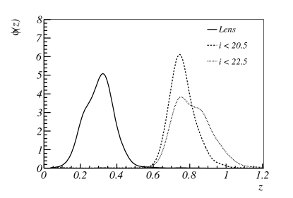
Figure 2: Redshift distributions from the stacking of the TPZ probability distribution functions for the lens and two i-band sub-samples of the source.

Photometric redshifts (photo-z) have been estimated using different techniques. In particular, the fiducial code used in this work employs a machine-learning algorithm (random forests) as implemented by TPZ (Carrasco Kind & Brunner, 2013), which was shown to perform well on SV data (Sánchez et al., 2014). The redshifts of the galaxies are defined according to the mean of the probability density functions given by TPZ ($z_{\rm ph}$). Other methods are also employed to demonstrate that the measured two-point angular cross-correlation are not a feature induced by TPZ (see subsection 6.2).

4.1 Lens sample

A unique lens sample is defined by the additional photo-z and magnitude cuts:

• $0.2<z_{\rm ph}<0.4$;

• $18.0<i<22.5$.

These requirements are imposed in order to be compatible with the first redshift bin of the so called ‘benchmark sample’ (Crocce et al., 2016). Note that the mag_auto cut along with the previous $i$-band depth cut guarantees uniformity (Crocce et al., 2016).

4.2 Source sample

Three source samples are defined, one per band:

• R: $0.7<z_{\rm ph}<1.0$ and $r<23.0$;

• I: $0.7<z_{\rm ph}<1.0$ and $i<22.5$;

• Z: $0.7<z_{\rm ph}<1.0$ and $z<22.0$.

Following the same approach we used on the lens, defined over the ‘benchmark’ sample, the mag_auto cut along with the previously defined depth cuts also guarantee uniformity on the corresponding band.

Within each R, I, Z source sample five sub-samples that map the magnitude evolution are defined,

• $\rm R_{1}$: $r<21.0$; $\rm R_{2}$: $r<21.5$; $\rm R_{3}$: $r<22.0$; $\rm R_{4}$: $r<22.5$; $\rm R_{5}$: $r<23.0$.

• $\rm I_{1}$: $i<20.5$; $\rm I_{2}$: $i<21.0$; $\rm I_{3}$: $i<21.5$; $\rm I_{4}$: $i<22.0$; $\rm I_{5}$: $i<22.5$.

• $\rm Z_{1}$: $z<20.0$; $\rm Z_{2}$: $z<20.5$; $\rm Z_{3}$: $z<21.0$; $\rm Z_{4}$: $z<21.5$; $\rm Z_{5}$: $z<22.0$.

Here $\rm S_{j}$ with $\rm j=1,2,3,4,5$ are the sub-samples of sample S with $\rm S\in\{R,I,Z\}$. In Figure 2, the redshift distributions of the lens and source sample are shown. Note that the sub-samples $\rm R_{5},I_{5},Z_{5}$ are equal to $\rm R,I,Z$ respectively.

The g-band is not used on this analysis because when the same approach is followed and a uniform sample is defined in that band, the number of galaxies of the lens and source samples decrease dramatically. This increases the shot noise preventing the measurement of number count magnification.

5 Application to a simulated galaxy survey

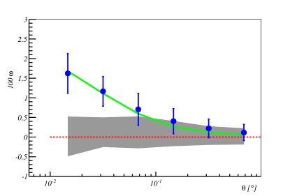
Figure 3: Two-point angular cross-correlation function for the MICE simulation (sample $i<21.5$). With magnification (dots) and without (grey shade), versus that expected from the MICE cosmological parameters, both with magnification (solid line) and without (dashed line), the latter being zero.

In order to test the methodology described above in a controlled environment, isolated from any source of systematic error, it is applied to a simulated galaxy sample, in particular MICECAT v1.0. This mock is the first catalog release of the N-body simulation MICE-GC (Fosalba et al., 2015a, b; Crocce et al., 2015). It assumes a flat $\Lambda$CDM Universe with cosmological parameters $\Omega_{M}=0.25,\Omega_{b}=0.044,h=0.7$ and $\sigma_{8}=0.8$, using a light-cone that spans one eighth of the celestial sphere. Another advantage of using these simulations is the possibility of studying specific systematic effects, as described in subsection 6.2.

Among other properties, MICE-GC provides lensed and unlensed coordinates, true redshift (including redshift space distortions) and DES-$griz$ unlensed magnitudes for the simulated galaxies, along with convergence and shear. Conversion from unlensed magnitudes to lensed magnitudes can be done by applying $m_{\mu}=m_{0}-2.5\log_{10}(1+2\kappa)$.

Having two sets of coordinates and magnitudes, one in a ‘universe’ with magnification and another without magnification, allows us to follow the methodology described in section 3 for both cases, serving as a test-bench to measure the sensitivity of the method to the magnification effect. In order to have a fiducial function with as little statistical uncertainty as possible, the full 5000 deg² of the MICE simulation are used. To match as much as possible the conditions of the DES-SV data, the magnitude cuts described in section 4 are applied to the lens and source samples. The covariance matrices of data (see subsection 6.1) are used, in order to match the errors in the DES-SV sample.

In Figure 3, the results of the magnification analysis in the MICE simulation for the cases with and without magnification can be seen compared with the theoretical expectations. The methodology used in this work clearly allows us to distinguish both cases for a data-set similar to that of the DES-SV data. Nevertheless, results obtained with the MICE simulation can not be directly extrapolated to SV data to estimate the expected significance because the density of galaxies on the simulation is a factor $\sim 3$ smaller than on the SV data. Also, the luminosity function of the simulation is slightly different from the DES data, which has a direct impact on the number count slope and, consequently, on the amplitude of the measured signal.

6 Data Analysis

The analysis of the SV data is described here, showing first the detection of the magnification signal followed by the study and correction of systematic effects.

6.1 Signal detection

To estimate the cross-correlation functions, the tree-code TreeCorr (Jarvis et al., 2004) and the Landy-Szalay estimator (Landy & Szalay, 1993) are used demanding six logarithmic angular bins:

$$\omega_{\rm LS_{j}}(\theta)=\frac{D_{\rm L}D_{\rm S_{j}}(\theta)-D_{\rm L}R_{\rm S_{j}}(\theta)-D_{\rm S_{j}}R_{\rm L}(\theta)}{R_{\rm L}R_{\rm S_{j}}(\theta)}+1,$$ (16)

where $D_{\rm L}D_{\rm S_{j}}(\theta)$ is the number of pairs from the lens data sample L and the source data sub-sample $\rm S_{j}$ separated by an angular distance $\theta$ and $D_{\rm L}R_{\rm S_{j}}(\theta)$, $D_{\rm S_{j}}R_{\rm L}(\theta)$, $R_{\rm L}R_{\rm S_{j}}(\theta)$ are the corresponding values for the lens-random, source-random and random-random combinations normalized by the total number of objects on each sample.

Catalogs produced with Balrog (Suchyta et al., 2016) are used as random samples. The Balrog catalogs are DES-like catalogs, where no intrinsic magnification signal has been included. The Balrog software generates images of fake objects, all with zero convergence $\kappa$, that are embedded into the DES-SV coadd images (convolving the objects with the measured point spread function, and applying the measured photometric calibration). Then SExtractor was run on them, using the same DES Data Management configuration parameters used for the image processing. The positions for the simulated objects were generated randomly over the celestial sphere, meaning that these positions are intrinsically unclustered. Hence, the detected Balrog objects amount to a set of random points, which sample the survey detection probability. For a full description and an application to the same measurement as in Crocce et al. (2016) see Suchyta et al. (2016). This is the first time that this extensive simulation is used to correct for systematics.

The same cuts and masking of the data sample (section 4) are also applied to the the Balrog sample. A re-weighting following a nearest-neighbours approach was applied to Balrog objects in order to follow the same magnitude distribution of the DES-SV data on both lens and sources.

A covariance matrix is computed for each band by jack-knife re-sampling the data taking into account the correlations between the different magnitude cut within each band

$$C_{\rm S}(\omega_{\rm LS_{i}}(\theta_{\eta});\omega_{\rm LS_{j}}(\theta_{\nu}))=\frac{N_{\rm JK}}{N_{\rm JK}-1}$$ (17)

$$\times\sum\limits_{k}^{N_{\rm JK}}[\omega_{\rm LS_{i}}^{k}(\theta_{\eta})-\omega_{\rm LS_{i}}(\theta_{\eta})][\omega_{\rm LS_{j}}^{k}(\theta_{\nu})-\omega_{\rm LS_{j}}(\theta_{\nu})],$$

where $\omega^{k}_{\rm LS_{j}}$ stands for the cross-correlation of the $k$-th jack-knife re-sample and $\omega_{\rm LS_{j}}$ is the cross-correlation of the full sample. The $N_{\rm JK}=120$ jack-knife regions are defined by a $k$-means algorithm (MacQueen et al., 1967) using Python’s machine learning library scikit-learn (Pedregosa et al., 2011). In order to get $N_{\rm JK}$ regions with equal area, the algorithm is trained on a uniform random sample following the footprint of the data demanding $N_{\rm JK}$ centres. The regions used on the re-sampling are composed by the Voronoi tessellation defined by these centres. These matrices trace the angular covariance as well as the covariances between functions within each band. No covariance between bands is considered, since each band is treated independently on this work. The reduced covariance matrix of the i-band is displayed at Figure 4. The behavior is similar for the other bands.

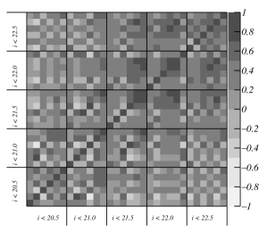
Figure 4: Covariance matrix of the i-band rescaled by the value of the diagonal ($C_{ij}/\sqrt{C_{ii}C_{jj}}$). Each box is the part of the matrix corresponding to the samples labeled at the axis whereas the bins within each box stand for the angular values of the correlation function.

Measured two-point angular cross-correlation functions and $\Lambda$CDM weak lensing theoretical predictions can be found in Figure 5. Measured correlation functions are found to be non-zero, compatible with $\Lambda$CDM and its amplitude evolves with the magnitude cut. The magnitude cuts imposed to guarantee uniform depth make that, for this data, no negative amplitudes are expected.

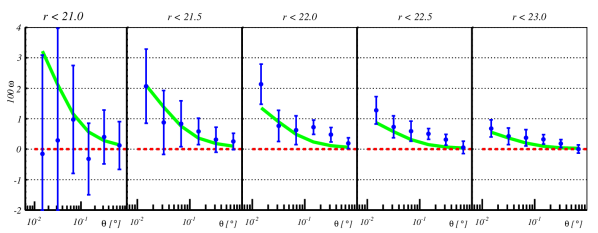
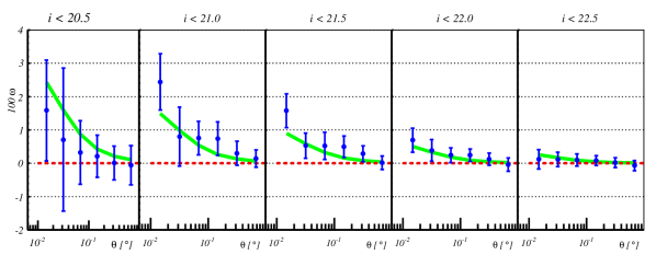
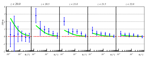
Figure 5: Measured cross-correlation functions (dots) of the lens sample with each source sample for the DES SVA1-Gold data using Balrog randoms. Each row corresponds to one of the R, I, Z source samples. Within each row, each sub-panel shows the cross-correlation with the flux limited source sub-sample indicated above. The solid line shows the theoretical prediction using expression Equation 15 computed assuming a $\Lambda$CDM Cosmology (Planck Collaboration, 2016) and the previously measured galaxy-bias $b_{\rm L}=1.07$ (Crocce et al., 2016). The dashed line is an eye-guide for zero.

To compare with the expected theory, Equation 13b has been used assuming Planck Collaboration (2016) cosmological parameters. The bias of the lens sample has already been measured independently with different techniques: clustering (Crocce et al., 2016), gg-lensing (Prat et al., 2016), shear (Chang et al., 2016) and CMB-lensing (Giannantonio et al., 2016). From these values the most precise, from Crocce et al. (2016), is selected ($b_{\rm L}=1.07\pm 0.08$) and is assumed to be a constant scale-independent parameter. The number count slope parameter $\alpha_{\rm S}$ is computed by fitting the cumulative number count of the sample S to a Schechter function (Schechter, 1976) on the range of interest

$$N_{\mu}(m)=A\left[10^{0.4(m-m_{*})}\right]^{\beta}\times\exp\left[-10^{0.4(m-m*)}\right],$$ (18)

where $A,m_{*},\beta$ are the free parameters of the fit. Then $\alpha_{\rm S}(m)-1$ is computed by applying Equation 9, where $m_{\rm j}$ is the magnitude limit of the $\rm S_{j}$ sub-sample on the considered band. In Figure 6 the fit and the number count slope parameter for the I sample are shown.

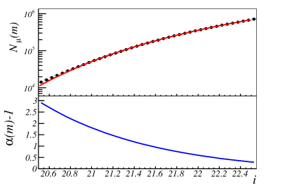
Figure 6: Top panel: Dots are the measured i-band cumulative number count as a function of the i-band magnitude. Red solid line is the fit using a Schechter function (see text). Bottom panel: number count slope $\alpha-1$ measured from the fitted Schechter function of the top panel.

Sample	$\log_{10}\mathcal{B}$	$\chi^{2}/ndof$	$\log_{10}\mathcal{B}$	$\chi^{2}/ndof$
$r<21.0$	-0.3	1.9/6
$r<21.5$	0.8	0.8/6
$r<22.0$	2.0	6.6/6	3.9	21.6/30
$r<22.5$	2.3	7.0/6
$r<23.0$	1.1	4.2/6
$i<20.5$	0.2	0.9/6
$i<21.0$	2.1	2.0/6
$i<21.5$	2.5	4.5/6	3.5	24.2/30
$i<22.0$	1.0	1.7/6
$i<22.5$	0.0	1.5/6
$z<20.0$	-0.4	2.6/6
$z<20.5$	2.3	2.6/6
$z<21.0$	2.6	8.8/6	3.9	37.9/30
$z<21.5$	0.9	3.5/6
$z<22.0$	0.5	2.1/6

Table 1: Significance of the detection of a magnification signal without weights. Significances determined by the logarithm of the Bayes factor and $\chi^{2}$ values of the expected theoretical signal are shown for each individual function as well for the combination of the five functions within a band (right).

Sample	$\log_{10}\mathcal{B}$	$\chi^{2}/ndof$
$r<23.0$	3.2	3.2/6
$i<22.5$	2.1	2.1/6
$z<22.0$	2.3	2.3/6

Table 2: Significance of the detection of a magnification signal with weights. Results are shown for the faintest sample.

A goodness of fit test of the measured two-point angular cross-correlation function respect to the theoretical predictions for each band is performed combining the five correlations functions within each band:

$$\chi^{2}_{\rm Planck}=\sum\limits_{\eta\nu ij}[\tilde{\omega}_{\rm LS_{i}}(\theta_{\eta})-\omega_{\rm LS_{i}}(\theta_{\eta})]$$ (19)

$$C^{-1}(\omega_{\rm LS_{i}}(\theta_{\eta});\omega_{\rm LS_{j}}(\theta_{\nu}))[\tilde{\omega}_{\rm LS_{j}}(\theta_{\nu})-\omega_{\rm LS_{j}}(\theta_{\nu})],$$ (20)

where $\tilde{\omega},\omega$ are the measured and theoretical cross-correlation functions respectively. Goodness of fit tests are also made testing the hypothesis of absence of magnification:

$$\chi^{2}_{\rm zero}=$$ (21)

$$\sum\limits_{\eta\nu ij}\tilde{\omega}_{\rm LS_{i}}(\theta_{\eta})C^{-1}(\omega_{\rm LS_{i}}(\theta_{\eta});\omega_{\rm LS_{j}}(\theta_{\nu}))\tilde{\omega}_{\rm LS_{j}}(\theta_{\nu}).$$

The $\chi^{2}$ values of the individual correlation functions as well as the combination of the five correlation functions within each band can be seen in Table 1 showing good agreement with the theoretical predictions described in section 2. To test which hypothesis is favored, the Bayes factor is used:

$$\mathcal{B}=\frac{P(M|\Theta)}{P(Z|\Theta)}=\frac{P(\Theta|M)}{P(\Theta|Z)}\frac{P(M)}{P(Z)},$$ (22)

where

$$P(M|\Theta)=e^{-\chi^{2}_{\rm Planck}/2}$$ (23)

and

$$P(Z|\Theta)=e^{-\chi^{2}_{\rm zero}/2}.$$ (24)

The assumed prior sets detection and non-detection of magnification to be equally probable: $P(M)=P(Z)$. Bayes factors are computed for each function individually as well as for each band using the full covariance.

The significance for each individual correlation function (see Table 1) has a strong dependence on the considered magnitude limit of the sub-sample. To compute the significance of the detection for each band, the five correlation functions within each and the full covariance are used. One covariance matrix (see Figure 4 for the i-band matrix) per each band is computed taking into account the full set of correlations. The logarithm of the Bayes factor can be found in Table 1, being all above 2, allowing to claim that magnification has been detected (Kass & Raftery, 1995).

A usual approach to enhance the signal-to-noise ratio, is to define a unique source sample, weight each source galaxy with its corresponding $\alpha_{S}(m)-1$ value (Ménard et al., 2003) and compute the two-point angular cross-correlation function. This weighting procedure is used at the samples $r<23.0$, $i<22.5$ and $z<22.0$. These correlation functions can be seen in Figure 7 with a comparison with the theoretical prediction and the correlation functions of the same sample computed without weighting. Significances of these measurement can be seen at Table 2 finding that the weighting approach provides an enhancement of the significance when compared with an unique sample. However, when the full set of correlation functions and their covariances are used, the results are similar since the same amount of data and information is used, that is, the number-count slope.

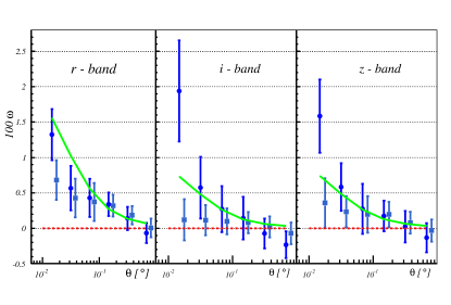
Figure 7: Measured two-point angular cross-correlation functions for the samples $r<23.0$, $i<22.5$ and $z<22.0$ left to right respectively. Dots use the optimal weighting (Scranton et al., 2005), where each galaxy is weighted by its corresponding $\alpha_{S}(m)-1$ value, whereas squares are not weighted. Green line is the theoretical prediction. Red dashed line is an eye-guide for zero.

Finally, in order to test that the signal is achromatic, the measured two-point angular cross-correlation functions for each band, normalized by its $\alpha_{S}(m)-1$ are compared. All cross-correlation functions fluctuate within $1\sigma$ errors (see Figure 8 for an example) demonstrating that the measured convergence field does not depend on the considered band.

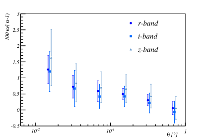
Figure 8: Example of the achromaticity of the measured signal. Here are shown the measured two-point angular cross-correlation functions for $r<22.5$, $i<22.0$ and $z<21.5$ divided by their corresponding $\alpha-1$.

6.2 Systematic errors

In this section, the impact of potential sources of systematic errors on the measured two-point angular cross-correlation function is investigated and how they are taken into account in the measurement is described.

6.2.1 Number count slope $\alpha$

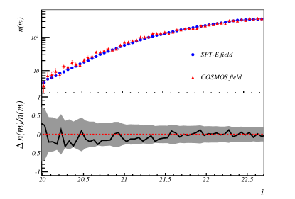
Figure 9: Upper panel: Comparison of the magnitude distribution for the SPT-E and the COSMOS fields. Both histograms are normalized by their respective area. Lower panel: Relative difference between the magnitude distribution of the COSMOS and the SPT-E fields. The shaded region shows the $1\sigma$ confidence interval computed from shot-noise.

When comparing the measured two point angular cross-correlation functions with the theoretical prediction via Equation 15 for a given set of cosmological parameters, $\alpha(m)$ is determined by fitting the cumulative number count distribution to Equation 18 and then using Equation 9. To compute the possible impact of the uncertainty of this fit on the comparison with theory, a marginalisation over all the parameters of the fit ($A,m_{*},\beta$) is made.

Parameters are randomly sampled with a Gaussian distribution centred on the value given by the fit to the cumulative number count and with a standard deviation equal to the $1\sigma$ errors of the fit. The value of $\alpha$ is recalculated with these randomly sampled parameters. The impact of the dispersion of the $\alpha$ values obtained is negligible compared to the size of the jackknife errors, so they are not taken into account.

In addition to the parameter determination, a possible non-completeness on the SPT-E field can modify the magnitude distribution altering the cumulative number count slope parameter (Hildebrandt, 2016). To estimate the possible impact of non-completeness, the measured magnitude distributions of the SPT-E field are compared with those of deeper fields measured by DES, such as the COSMOS field. Both distributions are found to be equal at the range of magnitudes considered on this analysis (see Figure 9 for an example in the $i$-band).

6.2.2 Object obscuration

Chang et al. (2015) studied whether moderately bright objects in crowded environments produce a decrease in the detection probability of nearby fainter objects at scales $\theta\lesssim 10\$arcsec. However, such scales are well below those considered in this analysis ($\theta>36$ arcsec) and therefore this effect is ignored.

6.2.3 Stellar contamination

For a given choice of star-galaxy classifier, there will be a number of stars misclassified as galaxies, so the observed two-point angular cross-correlation function $\omega_{O}(\theta)$ must be corrected by the presence of any fake signal induced by stars (see appendix A):

$$\omega_{\rm LS_{j}}=\frac{\omega_{\rm O}(\theta)-\lambda_{\rm L}\omega_{\rm*S_{j}}(\theta)-\lambda_{\rm S_{j}}\omega_{\rm L*}(\theta)}{1-\lambda_{\rm L}-\lambda_{\rm S_{j}}},$$ (25)

where $\omega_{\rm LS_{j}}$ is the corrected galaxy cross-correlation function, $\omega_{\rm L*}$ is the cross-correlation function of the true galaxy lenses with the stars misclassified as galaxies in the source sample, $\omega_{\rm*S_{j}}$ is the cross correlation of the stars misclassified as galaxies in the lenses with the true source galaxies and $\lambda_{\rm L},\lambda_{\rm S_{j}}$ are the fraction of stars in the lens and in the source samples respectively. Assuming that the misclassification of stars is spatially random and is a representative sample of the spatial distribution of the population classified as stars and that the fraction of misclassified stars is small, the functions $\omega_{\rm L*},\omega_{\rm*S_{j}}$ are estimated from the cross-correlation of the galaxy population and the stellar population in the corresponding redshift bin.

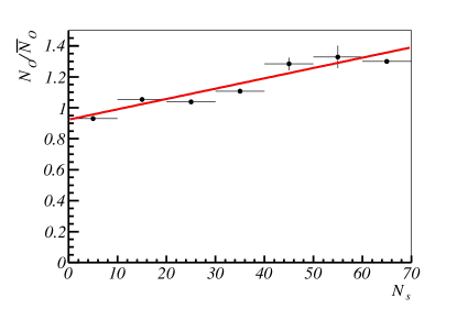
Figure 10: Determination of the purity of the lens sample. For each $N_{\rm nside}=512$ HEALPix-pixel, the number of objects classified as galaxies divided by the average number of galaxies per pixel is plotted as a function of the number of objects classified as stars. Black dots are the measured data. Red line is the linear fit to the data. The intercept of the line with the Y-axis is the estimated purity of the sample.

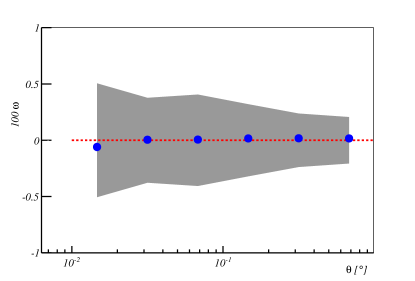
Figure 11: Correction by stellar contamination on the $i<21.5$ sample. Blue dots are the correction and shaded area is the $1\sigma$ confidence interval of the measured cross-correlations of the magnification signal. Red dashed line is and eye-guide for zero.

Following a similar approach to Ross et al. (2012), if the latter is true and the misclassified stars trace the global population of stars, for a given patch of the sky the number of objects classified as galaxies $N_{\rm O}$ must be the average number of true galaxies $\bar{N}_{\rm g}$ plus a quantity proportional to the number of stars on that given pixel,

$$N_{\rm O}=\bar{N}_{\rm g}+\tilde{\gamma}N_{\rm s}.$$ (26)

Dividing by the average number of objects marked as galaxies $\bar{N}_{\rm O}$,

$$\frac{N_{\rm O}}{\bar{N}_{\rm O}}=p+\gamma N_{\rm s},$$ (27)

where $p=\bar{N}_{\rm g}/\bar{N}_{\rm O}$ is the purity of the sample, that is, $\lambda=1-p$.

In order to estimate the purity of the galaxy sample with this method, an $N_{\rm side}=512$ HEALPix pixelation is made and for each pixel $N_{\rm O}/\bar{N}_{\rm O}$ and $N_{\rm s}$ is computed. Then, a fit to Equation 27 is made determining a purity of 94 per cent for the lens sample and about 98 per cent for the source sample depending on the considered band (see Figure 10 for an example). With this purity, the correction due to stellar contamination given by Equation 25 is found to be one order of magnitude smaller than the statistical errors (see Figure 11 for the $i$-band correction), so stellar contamination is not taken into account in the analysis. Nevertheless, on future analysis with more galaxies and area this may be important. Note that the objects labeled as stars by our star-galaxy classifier would be a combination of stars and galaxies thus these calculations are an upper bound to stellar contamination.

6.2.4 Survey observing conditions

Observing conditions are not constant during the survey, leading to spatial dependencies across the DES-SV footprint (Leistedt et al., 2015) that may affect the observed cross-correlation function, such as seeing variations, air-mass, sky-brightness or exposure time (Morrison & Hildebrandt, 2015). To trace these spatial variations, the catalog produced by the Monte Carlo sampling code Balrog has been used as random sample (Suchyta et al., 2016). It is important to remark that Balrog catalogs are produced with the same pipeline as DES-SV data, allowing one to trace subtle effects such as patchiness on the zeropoints, deblending and possible magnitude errors due to a wrong sky subtraction close to bright objects.

The use of Monte Carlo sampling methods provides a new approach to mitigate systematic effects complementary to methods that cross-correlate the galaxy-positions with the maps of the survey observing conditions (Ross et al., 2012; Ho et al., 2012; Morrison & Hildebrandt, 2015) or involve masking the regions of the sky with worst values of the observing conditions (Crocce et al., 2016). The amount of sky to be masked in order to mitigate the systematic effects on the correlation functions, is freely decided based on the impact on the correlation function, which may lead to a biassed measurement. On the other hand, the approach involving cross-correlations may lead to an overcorrection effect since the different maps of the observing conditions are, in general, correlated in a complicated manner (Elsner et al., 2016). This new Monte Carlo technique to sample the selection function of the survey given by Balrog, has the advantage that takes into account the correlation of the different observing conditions maps as well as provides an objective criteria to mitigate systematic errors on the correlation function for a given sample, avoiding biassed measurements. In addition, the use of Balrog has the potential to allow us in the future to exploit the full depth of the survey (Suchyta et al., 2016).

6.2.5 Dust extinction

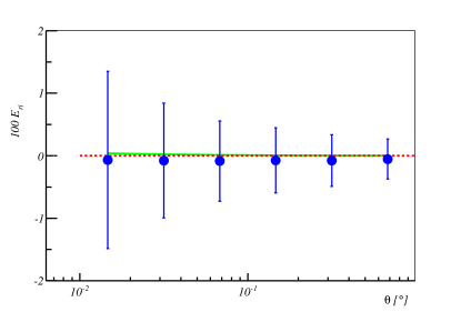
Figure 12: Blue dots: colour-density cross-correlation functions measured on SV data for the r and i bands (sample $i<21.5$). Green solid line is the expected value from Equation 31. Red dashed line is an eye-guide for zero.

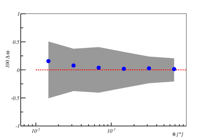
Figure 13: Impact of dust on the number count from MICE (case $i<21.5$). Shade is the $1\sigma$ confidence interval. Blue dots are the number count differences between the case with and the case without the simulated dust profile. Red dashed line is an eye-guide for zero.

The possible presence of dust in the lenses may modify the observed magnitude in addition to the magnitude shift due to magnification (Ménard et al., 2010). The change in magnitude ($\delta m$) on the $p$-band may be written as

$$\delta m_{p}=-2.5\log\mu+\frac{2.5}{\ln 10}\tau_{p},$$ (28)

where $\mu\simeq 1+2\kappa$ is the change in magnitude due to magnification and $\tau_{k}$ is the optical depth due to dust extinction. Whereas magnification is achromatic, dust extinction induces a band-dependent magnitude change. Taking this into account, the colour-excess for bands $p,q$ is defined as

$$E_{pq}=\delta m_{p}-\delta m_{q}=1.08[\tau_{p}-\tau_{q}].$$ (29)

Define the colour-density cross-correlation as (Ménard et al., 2010)

$$\langle\delta_{\rm g}E_{pq}\rangle(\theta)=1.09[\tau_{p}(\theta)-\tau_{q}(\theta)],$$ (30)

where $\delta_{\rm g}$ is the density contrast of the lenses and $E_{pq}$ is the colour-excess of the sources; from the measurements by Ménard et al. (2010) it can be parametrized as

$$\langle\delta_{\rm g}E_{pq}\rangle(\theta)=1.09\tau_{V}\left[\frac{\lambda_{V}}{\lambda_{p}}-\frac{\lambda_{V}}{\lambda_{q}}\right]\left(\frac{\theta}{1^{\prime}}\right)^{-0.8},$$ (31)

with $\tau_{V}=2.3\times 10^{-3}$ the optical depth at the V-band and $\lambda_{V},\lambda_{p},\lambda_{q}$ the average wavelengths of the $V$, $p$ and $q$ bands respectively. With this parametrization, the impact of dust extinction is negligible at the scales considered on this analysis. As it can be seen in Figure 12, colour-density cross-correlation functions are compatible with Equation 31 as well as with zero.

In addition, the impact of a dust profile has been simulated as described in Equation 31 with the MICE simulation (section 5). To do so, for each galaxy belonging to the source sample a magnitude shift is induced

$$m_{d}=m_{\mu}+1.09\tau_{V}\frac{\lambda_{V}}{\lambda}\sum\limits_{l}\left(\frac{\theta_{l}}{1^{\prime}}\right)^{-0.8}.$$ (32)

Here $\theta_{l}$ is the angular separation of the source-galaxy and the $l$-th lens galaxy and the summation is over all the galaxies of the lens sample. In Figure 13 the difference between the two-point angular cross-correlation with and without the dust can be seen to be less than the statistical errors. It can be deduced that dust has no impact on the angular scales considered on this work.

Since the parametrization used here only applies to a sample similar to the one used at Ménard et al. (2010), statements about dust constrains are limited. Nevertheless this does not change the fact that no chromatic effects are detected.

6.2.6 Photometric redshifts

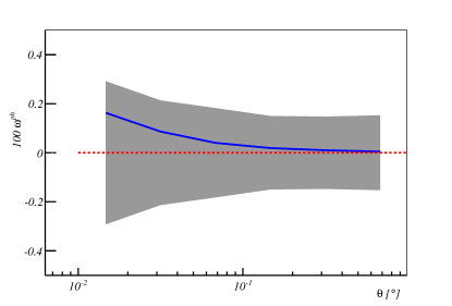
Figure 14: Comparison of $1\sigma$ jackknife errors of the measured correlation function (grey shade) with the expected signal induced by the photo-z migration between the lens and the source sample (case $i<22.5$) computed theoretically with the stacking of the pdfs for the $i$-band (blue line).

A general study of photo-z performance in DES-SV can be found in Sánchez et al. (2014). A comprehensive study of the photo-z performance and its implications for weak lensing can be found in Bonnett et al. (2016). Both studies are followed in this analysis. Conservative photo-z cuts are made in order to minimize the migration between lens and source samples. Nevertheless, catastrophic outliers in the photo-z determination can bias the measurement of $\kappa$ (Bernstein & Huterer, 2010). Thus, the tails of the probability density functions (pdfs) of the photo-z code are a crucial systematic to test. As mentioned in section 2, in addition to the magnification signal, galaxy migration due to a wrong photo-z assignment between lens and source samples may induce a non-zero cross-correlation signal due to the physical signal coming from the clustering of objects in the same redshift bin. As a first approach, estimation of the expected signal induced by photo-z migration ($\omega^{ph}$) is computed with Equation 13a:

$$\omega_{\rm LS_{j}}^{\rm ph}(\theta)=\int\limits_{0}^{\infty}dz\int\limits_{0}^{\infty}dz^{\prime}\phi_{\rm L}(z)\phi_{\rm S_{j}}(z^{\prime})\xi(\theta;z,z^{\prime}),$$ (33)

where $\xi(\theta;z,z^{\prime})$ is the 3D correlation-function and $\phi_{\rm L},\phi_{\rm S_{j}}$ are the redshift distribution of the lens (L) sample and the source sample ($\rm S_{j}$) estimated from the stacking of the pdfs given by TPZ. Figure 14 compares the measured two-point angular cross-correlation and the expected signal induced by photo-z can be seen for the I sample. The signal induced by photo-z is found to be smaller than the statistical errors. Note that this method relies on an assumed cosmology and bias model, and therefore should be considered only an approximation. A more accurate calculation can be made with the help of N-body simulations.

From the overlap of the redshift distribution of both lens and source samples, it is found that the total photo-z migration between lens and source sample is $o\sim 0.6\%$ depending on the magnitude cut of the source sample. The procedure to compute this overlap is to integrate the product of the pdfs of the lens and source sample:

$$o=\int\limits_{0}^{\infty}dz\phi_{L}(z)\phi_{S}(z),$$ (34)

where $\phi_{L},\phi_{S}$ are the stacked pdfs of the lens and source sample respectively. Since TPZ provides an individual pdf for each galaxy, the stacked pdf of a given sample is computed by adding all the individual pdfs of the galaxies that belong to that sample (see Asorey et al. (2016) for a study of clustering with stacked pdfs).

To estimate the maximum allowed photo-z migration between the lens and the source sample, the MICE simulation (section 5) with the un-lensed coordinates and magnitudes is used. Galaxies are randomly sampled on the lens redshift bin and then placed on the source redshift bin. Conversely, galaxies on the source redshift bin are randomly sampled and placed on the lens redshift bin. For a given lens or source sample, the number of galaxies introduced from the other redshift bin is chosen to be 0.1, 0.3, 0.5, 0.7, 0.9 and 2 per cent of the galaxies. Then, the two-point angular cross-correlation is computed for each case. The difference of the correlation functions measured at the simulation with induced migration between lens and source sample and the original used in section 5 is the signal induced by photo-z migration. The signal induced by photo-z for the cases with 0.9 and 2 per cent computed with this method can be seen at Figure 15. It is found that at 0.9 per cent of contamination, the induced signal due to photo-z migration is comparable to the error in the correlation functions. This upper limit is greater than the estimated photo-z migration, demonstrating that the effect of photo-z migration is negligible. Photo-z migration has a larger impact on the brightest samples. Nevertheless, since the errors of the correlation functions of these samples are shot-noise dominated, the tightest constraints on photo-z migration are imposed by the faintest samples. With a larger data sample this statement will no longer be true.

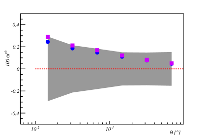
Figure 15: Estimation of the signal induced by migration of selected fractions of MICE un-lensed galaxies between the lens and the source sample (case $i<22.5$). Shaded area is the $1\sigma$ confidence interval for the measured number count cross-correlations. Dots correspond to a contamination fraction of 0.9 per cent. Squares correspond to a 2 per cent. Dashed line is an eye-guide for zero.

Photo-z induced correlation functions that mimic magnification may affect the measured significance. Thus, Bayes factor is recomputed with two new hypothesis, the measured signal is a combination of magnification and photo-z ($M+Ph$) or the measured signal is only photo-z ($Ph$):

$$\mathcal{B}=\frac{P(M+Ph|\Theta)}{P(Ph|\Theta)}=\frac{P(\Theta|M+Ph)}{P(\Theta|Ph)},$$ (35)

where

$$P(\Theta|M+Ph)=e^{-\chi^{2}_{\rm Planck+Ph}/2}$$ (36)

and

$$P(\Theta|Ph)=e^{-\chi^{2}_{\rm Ph}/2}.$$ (37)

To compute $\chi^{2}_{\rm Planck+Ph}$ and $\chi^{2}_{\rm Ph}$ it has been assumed that the expected theory is given by $\omega_{\rm LS_{j}}(\theta)+\omega_{\rm LS_{j}}^{\rm ph}(\theta)$ and $\omega_{\rm LS_{j}}^{\rm ph}$ respectively, where $\omega_{\rm LS_{j}}^{\rm ph}$ is the expected signal induced by photo-z computed using Equation 33. The significances recomputed using these two new hypothesis for the r, i and z bands are $\log_{10}\mathcal{B}=2.5,4.0,3.5$ respectively. Thus, it can be concluded that photo-z migration does not change the conclusions.

All previous calculations were based on the assumption that the pdfs are a reliable description of the true redshift distribution. This statement has been validated by previous works (Sánchez et al. (2014); Bonnett et al. (2016)). Redshift distributions predicted by TPZ are found to be representative of those given by the spectroscopic sample. Nevertheless, this statement has limitations –but is good enough for SV data– and a more accurate description of the real redshift distribution of the full sample will be measured with methodologies involving clustering-based estimators (Newman, 2008; Matthews & Newman, 2010; Ménard et al., 2013; Scottez et al., 2016) when the size of the data sample grows.

Finally, to demonstrate that the measured signal is independent of the photo-z technique employed to estimate the redshift, the two-point angular cross-correlation functions are measured using other estimators for photo-z, and have a performance similar to TPZ (Sánchez et al., 2014). A neural network, Skynet (Graff et al., 2014), and a template based approach, Bayesian Photo-Z (BPZ; Benítez (2000)) have been used. Figure 16 compares the cross-correlations computed with the three codes for the $i$-band, showing them to be within $1\sigma$ errors.

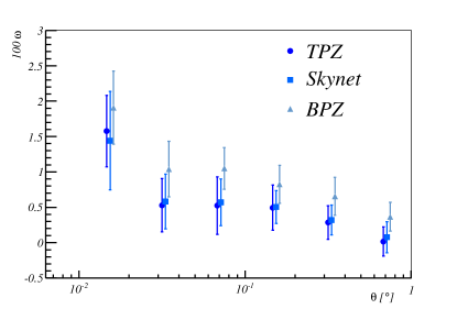
Figure 16: Comparison of the measured two-point angular cross-correlation functions corresponding to the sample $i<21.5$ measured with the Landy-Szalay estimator using TPZ, Skynet and BPZ. Triangles and squares are displaced at the horizontal axis for clarity.

7 Conclusions

In this paper weak lensing magnification of number count has been detected with the Dark Energy Survey, on each of the r, i, z photometric bands. The measured magnification signal agrees with theoretical predictions using a $\Lambda$CDM model with Planck Collaboration (2016) best-fit parameters.

This magnification measurement has been made using all measured galaxies, selecting them only by its photo-z. A method that makes explicit use of the full set of covariance matrices to maximize the significance has been used. The proposed method is compared with the usual weighting approach that can be found on the literature, reaching a similar level of significance. Although the methodology proposed on this work does not improve the signal-to-noise of the measurement of number-count magnification, allows a better control and estimation of systematic effects. Systematic effects due to observing conditions or photo-z have an strong correlation with the magnitudes of the galaxies. Thus, the weighted combination of galaxies leads to a non-trivial combination of correlated systematic effects. The proposed methodology analyzes independently the systematic effects of each set of galaxies combining afterwards the measured number-count magnification signal already corrected.

Systematic effects have been studied in detail not only using the data itself, but also supported with the N-body simulation MICE and the Balrog Monte Carlo sampling method. The use of Balrog provides a new and powerful way to deal with systematic errors complementary to usual approaches as masking and cross-correlations as it has been stated in subsubsection 6.2.4

The detection of magnification has been made only with 3 per cent of the final planned area for DES and half of the available maximum depth. This demonstrates that magnification measurements are feasible in the Dark Energy Survey and can provide an useful complement to the survey’s main goal on future data releases covering wider areas of the sky.

Future work will include the analysis of DES observations in much wider area, where some of the systematic issues not significant here such as stellar contamination and the accurate determination of the number count slope parameter, may not be negligible. These analyses will include measurements of cosmological parameters –by themselves or in combination with other weak lensing measurements (van Waerbeke, 2010)–, but also the other two effects of magnification: the observed magnitude shift (Ménard et al., 2010) and the increase in the observed size (Huff & Graves, 2014).

Appendix A Influence of Stellar Contamination on the Two-Point Angular Cross-Correlation

The observed density contrast of objects is given by

$$\delta_{\rm O}(\boldsymbol{\hat{n}},z_{i})=\frac{N_{\rm g}(z_{i})+N_{*}(z_{i})}{\bar{N}_{\rm g}(z_{i})+\bar{N}_{*}(z_{i})}-1,$$ (38)

where $N_{\rm g},N_{*}$ are the number of galaxies on direction $\boldsymbol{\hat{n}}$ and redshift $z_{i}$ and stars respectively and $\bar{N}_{\rm g},\bar{N}_{*}$ the average number of galaxies and stars over the footprint. The previous equation can be expressed as

$$\delta_{\rm O}(\boldsymbol{\hat{n}},z_{i})=\frac{N_{\rm g}(z_{i})+N_{*}(z_{i})}{\bar{N}_{\rm g}(z_{i})\left[1+\frac{\bar{N}_{*}(z_{i})}{\bar{N}_{\rm g}(z_{i})}\right]}-1.$$ (39)

Taylor expanding the brackets one has,

$$\delta_{\rm O}(\boldsymbol{\hat{n}},z_{i})=\frac{N_{\rm g}(z_{i})+N_{*}(z_{i})}{\bar{N}_{\rm g}(z_{i})}\left[1-\frac{\bar{N}_{*}(z_{i})}{\bar{N}_{\rm g}(z_{i})}\right]-1$$ (40)

and taking common factor $\bar{N}_{*}(z_{i})/\bar{N}_{\rm g}(z_{i})$,

$$\delta_{\rm O}(z_{i})=\left[\frac{N_{\rm g}(z_{i})}{\bar{N}_{\rm g}(z_{i})}-1\right]+$$ (41)

$$\frac{\bar{N}_{*}(z_{i})}{\bar{N}_{\rm g}(z_{i})}\left[\frac{N_{*}(z_{i})}{\bar{N}_{*}(z_{i})}-\frac{N_{\rm g}(z_{i})}{\bar{N}_{\rm g}(z_{i})}\right]-\frac{N_{*}(z_{i})}{\bar{N}_{\rm g}(z_{i})}.$$

Assuming that $\bar{N}_{*}\ll\bar{N}_{g}$, the last term can be neglected and defining $\lambda_{i}=\bar{N}_{*}(z_{i})/\bar{N}_{\rm g}(z_{i})$ as the fraction of stars on the $i$-th sample,

$$\delta_{\rm O}(\boldsymbol{\hat{n}},z_{i})=\delta_{\rm g}(\boldsymbol{\hat{n}},z_{i})+\lambda_{i}[\delta_{*}(\boldsymbol{\hat{n}},z_{i})-\delta_{\rm g}(\boldsymbol{\hat{n}},z_{i})].$$ (42)

Calculating the two point angular cross-correlation results finally in

$$\omega_{\rm O}=(1-\lambda_{i}-\lambda_{j})\omega_{\rm gg}+\lambda_{j}\omega_{\rm g*}+\lambda_{i}\omega_{\rm*g}+\lambda_{i}\lambda_{j}\omega_{**}.$$ (43)

AFFILIATIONS

¹ Centro de Investigaciones Energéticas, Medioambientales y Tecnológicas (CIEMAT), Madrid, Spain
² Computer Science and Mathematics Division, Oak Ridge National Laboratory, Oak Ridge, TN 37831
³ Jet Propulsion Laboratory, California Institute of Technology, 4800 Oak Grove Dr., Pasadena, CA 91109, USA
⁴ Institut de Ciències de l’Espai, IEEC-CSIC, Campus UAB, Carrer de Can Magrans, s/n, 08193 Bellaterra, Barcelona, Spain
⁵ Institut de Física d’Altes Energies (IFAE), The Barcelona Institute of Science and Technology, Campus UAB, 08193 Bellaterra (Barcelona) Spain
⁶ Universitäts-Sternwarte, Fakultät für Physik, Ludwig-Maximilians Universität München, Scheinerstr. 1, 81679 München, Germany
⁷ Cerro Tololo Inter-American Observatory, National Optical Astronomy Observatory, Casilla 603, La Serena, Chile
⁸ Department of Physics & Astronomy, University College London, Gower Street, London, WC1E 6BT, UK
⁹ Department of Physics and Electronics, Rhodes University, PO Box 94, Grahamstown, 6140, South Africa
¹⁰ Fermi National Accelerator Laboratory, P. O. Box 500, Batavia, IL 60510, USA
¹¹ CNRS, UMR 7095, Institut d’Astrophysique de Paris, F-75014, Paris, France
¹² Sorbonne Universités, UPMC Univ Paris 06, UMR 7095, Institut d’Astrophysique de Paris, F-75014, Paris, France
¹³ Department of Physics and Astronomy, University of Pennsylvania, Philadelphia, PA 19104, USA
¹⁴ Kavli Institute for Particle Astrophysics & Cosmology, P. O. Box 2450, Stanford University, Stanford, CA 94305, USA
¹⁵ SLAC National Accelerator Laboratory, Menlo Park, CA 94025, USA
¹⁶ Laboratório Interinstitucional de e-Astronomia - LIneA, Rua Gal. José Cristino 77, Rio de Janeiro, RJ - 20921-400, Brazil
¹⁷ Observatório Nacional, Rua Gal. José Cristino 77, Rio de Janeiro, RJ - 20921-400, Brazil
¹⁸ Department of Astronomy, University of Illinois, 1002 W. Green Street, Urbana, IL 61801, USA
¹⁹ National Center for Supercomputing Applications, 1205 West Clark St., Urbana, IL 61801, USA
²⁰ Institute of Cosmology & Gravitation, University of Portsmouth, Portsmouth, PO1 3FX, UK
²¹ School of Physics and Astronomy, University of Southampton, Southampton, SO17 1BJ, UK
²² George P. and Cynthia Woods Mitchell Institute for Fundamental Physics and Astronomy, and Department of Physics and Astronomy, Texas A&M University, College Station, TX 77843, USA
²³ Department of Physics, IIT Hyderabad, Kandi, Telangana 502285, India
²⁴ Department of Astronomy, University of Michigan, Ann Arbor, MI 48109, USA
²⁵ Department of Physics, University of Michigan, Ann Arbor, MI 48109, USA
²⁶ Kavli Institute for Cosmological Physics, University of Chicago, Chicago, IL 60637, USA
²⁷ Instituto de Física Teórica IFT-UAM/CSIC Universidad Autónoma de Madrid, Cantoblanco 28049, Madrid, Spain
²⁸ Institute of Astronomy, University of Cambridge, Madingley Road, Cambridge CB3 0HA, UK
²⁹ Kavli Institute for Cosmology, University of Cambridge, Madingley Road, Cambridge CB3 0HA, UK
³⁰ Astronomy Department, University of Washington, Box 351580, Seattle, WA 98195, USA
³¹ Australian Astronomical Observatory, North Ryde, NSW 2113, Australia
³² Departamento de Física Matemática, Instituto de Física, Universidade de São Paulo, CP 66318, CEP 05314-970, São Paulo, SP, Brazil
³³ Jodrell Bank Center for Astrophysics, School of Physics and Astronomy, University of Manchester, Oxford Road, Manchester, M13 9PL, UK
³⁴ Department of Astrophysical Sciences, Princeton University, Peyton Hall, Princeton, NJ 08544, USA
³⁵ Institució Catalana de Recerca i Estudis Avançats, E-08010 Barcelona, Spain
³⁶ Excellence Cluster Universe, Boltzmannstr. 2, 85748 Garching, Germany
³⁷ Faculty of Physics, Ludwig-Maximilians-Universität, Scheinerstr. 1, 81679 Munich, Germany
³⁸ Max Planck Institute for Extraterrestrial Physics, Giessenbachstrasse, 85748 Garching, Germany
³⁹ Department of Physics and Astronomy, Pevensey Building, University of Sussex, Brighton, BN1 9QH, UK
⁴⁰ Universidade Federal do ABC, Centro de Ciências Naturais e Humanas, Av. dos Estados, 5001, Santo André, SP, Brazil, 09210-580

References

- Asorey et al. (2016) Asorey J., Carrasco Kind M., Sevilla-Noarbe I., Brunner R. J., Thaler J., 2016, MNRAS, 459, 1293
- Bartelmann (1992a) Bartelmann M., 1992a, in Klare G., ed., Reviews in Modern Astronomy Vol. 5, Reviews in Modern Astronomy. pp 259–270
- Bartelmann (1992b) Bartelmann M., 1992b, Sterne und Weltraum, 31, 459
- Bartelmann (1992c) Bartelmann M., 1992c, in Kayser R., Schramm T., Nieser L., eds, Lecture Notes in Physics, Berlin Springer Verlag Vol. 406, Gravitational Lenses. p. 345, doi:10.1007/3-540-55797-0˙122
- Bartelmann (1995a) Bartelmann M., 1995a, A&A, 298, 661
- Bartelmann (1995b) Bartelmann M., 1995b, A&A, 303, 643
- Bartelmann & Narayan (1995) Bartelmann M., Narayan R., 1995, in Holt S. S., Bennett C. L., eds, American Institute of Physics Conference Series Vol. 336, Dark Matter. pp 307–319 (arXiv:astro-ph/9411033), doi:10.1063/1.48350
- Bartelmann & Schneider (1992) Bartelmann M., Schneider P., 1992, A&A, 259, 413
- Bartelmann & Schneider (1993) Bartelmann M., Schneider P., 1993, A&A, 268, 1
- Bartelmann & Schneider (2001) Bartelmann M., Schneider P., 2001, Phys. Rep., 340, 291
- Bauer et al. (2014) Bauer A. H., Gaztañaga E., Martí P., Miquel R., 2014, MNRAS, 440, 3701
- Benítez (2000) Benítez N., 2000, ApJ, 536, 571
- Bernstein & Huterer (2010) Bernstein G., Huterer D., 2010, MNRAS, 401, 1399
- Bertin & Arnouts (1996) Bertin E., Arnouts S., 1996, A&AS, 117, 393
- Blandford & Narayan (1992) Blandford R. D., Narayan R., 1992, ARA&A, 30, 311
- Blandford et al. (1989) Blandford R. D., Kochanek C. S., Kovner I., Narayan R., 1989, Science, 245, 824
- Bonnett et al. (2016) Bonnett C., et al., 2016, Phys. Rev. D, 94, 042005
- Broadhurst (1995) Broadhurst T., 1995, in Holt S. S., Bennett C. L., eds, American Institute of Physics Conference Series Vol. 336, Dark Matter. pp 320–329 (arXiv:astro-ph/9505010), doi:10.1063/1.48351
- Carrasco Kind & Brunner (2013) Carrasco Kind M., Brunner R. J., 2013, MNRAS, 432, 1483
- Chang et al. (2015) Chang C., et al., 2015, The Astrophysical Journal, 801, 73
- Chang et al. (2016) Chang C., et al., 2016, MNRAS, 459, 3203
- Chiu et al. (2016) Chiu I., et al., 2016, MNRAS, 457, 3050
- Clerkin et al. (2015) Clerkin L., Kirk D., Lahav O., Abdalla F. B., Gaztañaga E., 2015, MNRAS, 448, 1389
- Crocce et al. (2015) Crocce M., Castander F. J., Gaztañaga E., Fosalba P., Carretero J., 2015, MNRAS, 453, 1513
- Crocce et al. (2016) Crocce M., et al., 2016, MNRAS, 455, 4301
- Desai et al. (2012) Desai S., et al., 2012, ApJ, 757, 83
- Diehl (2012) Diehl T., 2012, Physics Procedia, 37, 1332
- Elsner et al. (2016) Elsner F., Leistedt B., Peiris H. V., 2016, MNRAS, 456, 2095
- Flaugher (2005) Flaugher B., 2005, International Journal of Modern Physics A, 20, 3121
- Flaugher et al. (2015) Flaugher B., et al., 2015, AJ, 150, 150
- Ford et al. (2014) Ford J., Hildebrandt H., Van Waerbeke L., Erben T., Laigle C., Milkeraitis M., Morrison C. B., 2014, MNRAS, 439, 3755
- Fosalba et al. (2015a) Fosalba P., Gaztañaga E., Castander F. J., Crocce M., 2015a, MNRAS, 447, 1319
- Fosalba et al. (2015b) Fosalba P., Crocce M., Gaztañaga E., Castander F. J., 2015b, MNRAS, 448, 2987
- Fugmann (1990) Fugmann W., 1990, A&A, 240, 11
- Gaztañaga (2003) Gaztañaga E., 2003, The Astrophysical Journal, 589, 82
- Giannantonio et al. (2016) Giannantonio T., et al., 2016, MNRAS, 456, 3213
- Górski et al. (2005) Górski K. M., Hivon E., Banday A. J., Wandelt B. D., Hansen F. K., Reinecke M., Bartelmann M., 2005, ApJ, 622, 759
- Graff et al. (2014) Graff P., Feroz F., Hobson M. P., Lasenby A., 2014, MNRAS, 441, 1741
- Grossman & Narayan (1989) Grossman S. A., Narayan R., 1989, ApJ, 344, 637
- Hildebrandt (2016) Hildebrandt H., 2016, MNRAS, 455, 3943
- Hildebrandt et al. (2009) Hildebrandt H., van Waerbeke L., Erben T., 2009, A&A, 507, 683
- Ho et al. (2012) Ho S., et al., 2012, ApJ, 761, 14
- Hoekstra & Jain (2008) Hoekstra H., Jain B., 2008, Annual Review of Nuclear and Particle Science, 58, 99
- Hogan et al. (1989) Hogan C. J., Narayan R., White S. D. M., 1989, Nature, 339, 106
- Huff & Graves (2014) Huff E. M., Graves G. J., 2014, The Astrophysical Journal Letters, 780, L16
- Hui et al. (2007) Hui L., Gaztañaga E., LoVerde M., 2007, Phys. Rev. D, 76, 103502
- Hui et al. (2008) Hui L., Gaztañaga E., LoVerde M., 2008, Phys. Rev. D, 77, 063526
- Jain & Lima (2011) Jain B., Lima M., 2011, MNRAS, 411, 2113
- Jarvis et al. (2004) Jarvis M., Bernstein G., Jain B., 2004, MNRAS, 352, 338
- Kaiser (1984) Kaiser N., 1984, ApJ, 284, L9
- Kass & Raftery (1995) Kass R. E., Raftery A. E., 1995, Journal of the American Statistical Association, 90, 773
- Kilbinger (2015) Kilbinger M., 2015, Reports on Progress in Physics, 78, 086901
- Landy & Szalay (1993) Landy S. D., Szalay A. S., 1993, ApJ, 412, 64
- Leistedt et al. (2015) Leistedt B., et al., 2015, preprint, (arXiv:1507.05647)
- LoVerde et al. (2008) LoVerde M., Hui L., Gaztañaga E., 2008, Phys. Rev. D, 77, 023512
- MacQueen et al. (1967) MacQueen J., et al., 1967, in Proceedings of the fifth Berkeley symposium on mathematical statistics and probability. pp 281–297
- Mandelbaum et al. (2005) Mandelbaum R., et al., 2005, MNRAS, 361, 1287
- Matthews & Newman (2010) Matthews D. J., Newman J. A., 2010, ApJ, 721, 456
- Ménard & Bartelmann (2002) Ménard B., Bartelmann M., 2002, A&A, 386, 784
- Ménard et al. (2003) Ménard B., Hamana T., Bartelmann M., Yoshida N., 2003, A&A, 403, 817
- Ménard et al. (2010) Ménard B., Scranton R., Fukugita M., Richards G., 2010, MNRAS, 405, 1025
- Ménard et al. (2013) Ménard B., Scranton R., Schmidt S., Morrison C., Jeong D., Budavari T., Rahman M., 2013, preprint, (arXiv:1303.4722)
- Meylan et al. (2006) Meylan G., Jetzer P., North P., Schneider P., Kochanek C. S., Wambsganss J., eds, 2006, Gravitational Lensing: Strong, Weak and Micro (arXiv:astro-ph/0407232)
- Mohr et al. (2012) Mohr J. J., et al., 2012, in Software and Cyberinfrastructure for Astronomy II. p. 84510D (arXiv:1207.3189), doi:10.1117/12.926785
- Morrison & Hildebrandt (2015) Morrison C. B., Hildebrandt H., 2015, MNRAS, 454, 3121
- Morrison et al. (2012) Morrison C. B., Scranton R., Ménard B., Schmidt S. J., Tyson J. A., Ryan R., Choi A., Wittman D. M., 2012, MNRAS, 426, 2489
- Narayan (1989) Narayan R., 1989, ApJ, 339, L53
- Narayan & Wallington (1993) Narayan R., Wallington S., 1993, in Surdej J., Fraipont-Caro D., Gosset E., Refsdal S., Remy M., eds, Liege International Astrophysical Colloquia Vol. 31, Liege International Astrophysical Colloquia. p. 217
- Newman (2008) Newman J. A., 2008, ApJ, 684, 88
- Peacock & Dodds (1994) Peacock J. A., Dodds S. J., 1994, MNRAS, 267, 1020
- Pedregosa et al. (2011) Pedregosa F., et al., 2011, Journal of Machine Learning Research, 12, 2825
- Planck Collaboration (2016) Planck Collaboration 2016, A&A, 594, A13
- Prat et al. (2016) Prat J., et al., 2016, preprint, (arXiv:1609.08167)
- Ross et al. (2012) Ross A. J., et al., 2012, MNRAS, 424, 564
- Sánchez et al. (2014) Sánchez C., et al., 2014, MNRAS, 445, 1482
- Schechter (1976) Schechter P., 1976, ApJ, 203, 297
- Scottez et al. (2016) Scottez V., et al., 2016, MNRAS, 462, 1683
- Scranton et al. (2005) Scranton R., et al., 2005, The Astrophysical Journal, 633, 589
- Seldner & Peebles (1979) Seldner M., Peebles P. J. E., 1979, ApJ, 227, 30
- Sevilla et al. (2011) Sevilla I., et al., 2011, preprint, (arXiv:1109.6741)
- Suchyta et al. (2016) Suchyta E., et al., 2016, MNRAS, 457, 786
- Swanson et al. (2008) Swanson M. E. C., Tegmark M., Hamilton A. J. S., Hill J. C., 2008, MNRAS, 387, 1391
- Wang et al. (2011) Wang L., et al., 2011, MNRAS, 414, 596
- Weinberg et al. (2013) Weinberg D. H., Mortonson M. J., Eisenstein D. J., Hirata C., Riess A. G., Rozo E., 2013, Physics Reports, 530, 87
- White & Rees (1978) White S. D. M., Rees M. J., 1978, MNRAS, 183, 341
- van Waerbeke (2010) van Waerbeke L., 2010, MNRAS, 401, 2093
- van Waerbeke et al. (2010) van Waerbeke L., Hildebrandt H., Ford J., Milkeraitis M., 2010, The Astrophysical Journal Letters, 723, L13