Univariate log-concave density estimation with symmetry or modal constraints

Abstract

We study nonparametric maximum likelihood estimation of a log-concave density function $f_{0}$ which is known to satisfy further constraints, where either (a) the mode $m$ of $f_{0}$ is known, or (b) $f_{0}$ is known to be symmetric about a fixed point $m$. We develop asymptotic theory for both constrained log-concave maximum likelihood estimators (MLE’s), including consistency, global rates of convergence, and local limit distribution theory. In both cases, we find the MLE’s pointwise limit distribution at $m$ (either the known mode or the known center of symmetry) and at a point $x_{0}\neq m$. Software to compute the constrained estimators is available in the R package logcondens.mode.

The symmetry-constrained MLE is particularly useful in contexts of location estimation. The mode-constrained MLE is useful for mode-regression. The mode-constrained MLE can also be used to form a likelihood ratio test for the location of the mode of $f_{0}$. These problems are studied in separate papers. In particular, in a separate paper we show that, under a curvature assumption, the likelihood ratio statistic for the location of the mode can be used for hypothesis tests or confidence intervals that do not depend on either tuning parameters or nuisance parameters.

mylongform mynotes

and label=u1,url]http://www.stat.washington.edu/jaw/ t1Supported in part by NSF Grants DMS-1104832 and a University of Minnesota Grant-In-Aid grant. t2Supported in part by NSF Grants DMS-1104832 and DMS-1566514, and NI-AID grant 2R01 AI291968-04

1 Introduction and overview

The classes of log-concave densities on ${\mathbb{R}}$ (and on ${\mathbb{R}}^{d}$) have great importance in statistics for a variety of reasons including their many natural closure properties, including closure under convolution, affine transformations, convergence in distribution, and marginalization. These classes are also unimodal and serve as important nonparametric generalizations of the class of Gaussian distributions.

Nonparametric estimation in the unconstrained classes of log-concave densities has developed rapidly in the past 10–15 years. Existence of maximum likelihood estimators for log-concave densities on ${\mathbb{R}}$ was provided by Walther (2002), while Pal, Woodroofe and Meyer (2007) established consistency. Dümbgen and Rufibach (2009) gave rates of convergence in certain uniform metrics, and provided efficient algorithms based on “active set” methods (see also Dümbgen and Rufibach (2011)). Balabdaoui, Rufibach and Wellner (2009) established pointwise limit distribution theory for the MLE’s, while Doss and Wellner (2016) established rates of convergence of the MLE in the Hellinger metric. There has also been rapid progress in estimation of log-concave densities on ${\mathbb{R}}^{d}$; see e.g. Cule, Samworth and Stewart (2010), Cule and Samworth (2010), Dümbgen, Samworth and Schuhmacher (2011), Seregin and Wellner (2010), and Han and Wellner (2016).

Interesting uses of the unconstrained log-concave MLE’s in more complicated models, mostly in mixture modeling and clustering, have been considered by Chang and Walther (2007), Eilers and Borgdorff (2007), Walther (2009), and Cule and Samworth (2010).

On the other hand, for a number of important statistical problems it is of great interest to understand estimation in several important sub-classes of the class of all log-concave densities on ${\mathbb{R}}$.

• For testing that a log-concave density on ${\mathbb{R}}$ is symmetric about a known point, for example $0$, we need know how to estimate the log-concave density both with and without the constraint of symmetry.

• For the basic problem of estimation of location with a symmetric error density, it is important to know how to estimate a symmetric log-concave density with mode (and median and mean) equal to $0$.

• For inference about the mode of a log-concave density it is necessary to understand how to estimate a log-concave density with a known mode $m$ (but without the constraint of symmetry).

Once the properties of nonparametric estimators within these sub-classes is understood, then the estimators can be used to develop statistical methods with known properties for other more complex statistical problems. For example: the basic procedures we study here can be viewed as building blocks to be used for, among others:

(a)

Testing the hypothesis of symmetry of a log-concave density.

(b)

Estimation of the location of a symmetric log-concave density.

(c)

Inference about the mode of a log-concave density.

(d)

Nonparametric modal regression (as in Chen et al. (2016), but using log-concavity).

(e)

Semiparametric estimation in mixture models based on symmetric log-concave distributions; see e.g. Balabdaoui and Doss (2018), Pu and Arias-Castro (2017), and Eilers and Borgdorff (2007).

(f)

Modal clustering (as in Chacón (2018a), but using log-concavity).

(g)

Estimation of a spherically symmetric multivariate log-concave density, which is pursued in Xu and Samworth (2017).

(h)

Inference about the center of an elliptical multivariate distribution based on the assumption of a log-concave underlying shape.

Thus our focus here is on estimation of a log-concave density in two important sub-classes: Let $\mathcal{LC}$ denote the class of all log-concave densities on the real line ${\mathbb{R}}$. The two subclasses we study here are:
(1) The class $\mathcal{LC}(m)=\mathcal{LC}_{m}$ of all log-concave densities with mode a
      fixed number $m$.
(2) The class $\mathcal{SLC}(0)=\mathcal{SLC}_{0}$ of all log-concave densities symmetric at $0$.

We let $\hat{f}_{n}^{0}$ denote the maximum likelihood estimator of $f_{0}\in{\cal LC}_{m}$ based on an i.i.d. sample $X_{1},\ldots,X_{n}$ from $f_{0}$; and we let $\hat{g}_{n}^{0}$ denote the maximum likelihood estimator of $g_{0}\in{SLC}_{0}$, based on an i.i.d. sample from $g_{0}$.

We rely on the methods and properties developed here for the subclass $\mathcal{LC}(m)$ to derive new inference procedures for the mode in Doss and Wellner (2019). The sub-class $\mathcal{SLC}(0)$ has already been used in Balabdaoui and Doss (2018) to study semiparametric mixture models. The methods developed here for $\mathcal{SLC}(0)$ are also being used in an on-going study by Laha (2019) of efficient estimation of a location parameter in the classical semiparametric symmetric location model with the (very natural) assumption of a symmetric log-concave error distribution. Methodology based on modes or local maxima of nonparametrically estimated functions has seen a resurgence in recent years; see, e.g., Chen et al. (2016), Chen, Genovese and Wasserman (2015), and Qiao and Polonik (2016). A recent survey on estimation and inference for the mode and on mode-based methodology is given by Chacón (2018b).

Thus our main goals here are the following:

1. To show that the mode-constrained MLE’s $\hat{f}_{n}^{0}\in\mathcal{LC}(m)$ and $\hat{g}_{n}^{0}\in\mathcal{SLC}(0)$ exist and to provide useful characterizations thereof.

2. Establish useful finite-sample properties of $\hat{f}_{n}^{0}$ and $\hat{g}_{n}^{0}$.

3. Establish consistency of the mode-constrained and symmetric mode-constrained MLE’s with respect to the Hellinger metric.

4. Establish local rates of convergence of the constrained estimators $\hat{f}_{n}^{0}$ and $\hat{g}_{n}^{0}$ and establish the (pointwise) asymptotic distributions of the constrained estimators.

5. Establish global rates of convergence of the constrained estimators.

Here is a brief summary of the paper: In Section 2 we show that the constrained estimators exist and satisfy useful characterizations. Section 3 provides plots of the constrained estimators and provides comparisons to each other and to the unconstrained maximum likelihood estimators $\hat{f}_{n}\in\mathcal{LC}$. In Section 4 we summarize results concerning consistency and global rates of convergence, while Section 5 addresses local rates of convergence and limiting distributions at fixed points. Section 6 summarizes some problems and difficulties concerning extensions to higher dimensions. All the proofs are given in the Appendix.

Many of our theorems have parts labeled “A”, “B”, and “C.” In general the “A parts” of results here have been proved by other authors (as noted in the theorem statements), the “B parts” were proved (for the most part) in the University of Washington Ph.D. dissertation of the first author, Doss (2013b). The “C parts” are new findings by the present authors, whose proofs are in some cases (as noted in text near the corresponding results) related to proofs developed by Balabdaoui and Doss (2018).

2 Maximum likelihood estimator finite sample properties: unconstrained and mode-constrained

2.1 Notation and terminology

Several classes of concave functions will play a central role in this paper. In particular, we let

$${\cal C}:=\{\varphi:\ {\mathbb{R}}\rightarrow[-\infty,\infty)\ |\ \varphi\ \ \mbox{is concave, closed, and proper}\}$$ (2.1)

and, for any fixed $m\in{\mathbb{R}}$,

$${\cal C}_{m}:=\{\varphi\in{\cal C}\ |\ \varphi(m)\geq\varphi(x)\ \ \mbox{for all}\ \ x\in{\mathbb{R}}\}$$ (2.2)

is the class of concave functions on ${\mathbb{R}}$ with mode at $m$. We also let

$${\cal SC}_{0}:=\{\varphi\in{\cal C}_{0}\ |\ \varphi(-x)=\varphi(x)\ \ \mbox{for all}\ \ x\in{\mathbb{R}}\}.$$ (2.3)

Here proper and closed concave functions are as defined in Rockafellar (1970), pages 24 and 50. We will follow the convention that all concave functions $\varphi$ are defined on all of ${\mathbb{R}}$ and take the value $-\infty$ off of their effective domains where $\mbox{dom}(\varphi):=\{x\ :\ \varphi(x)>-\infty\}$ (Rockafellar (1970), page 40). The classes of unconstrained and constrained log-concave densities are then

$${\cal LC}:=\left\{e^{\varphi}\ :\ \int e^{\varphi}d\lambda=1,\ \ \varphi\in{\cal C}\right\},$$

$${\cal LC}_{m}:=\left\{e^{\varphi}\ :\ \int e^{\varphi}d\lambda=1,\ \ \varphi\in{\cal C}_{m}\right\},\ \ \ \mbox{and}$$

$${\cal SLC}_{0}:=\left\{e^{\varphi}\ :\int e^{\varphi}d\lambda=1,\ \ \varphi\in{\cal SC}_{0}\right\},$$

where $\lambda$ is Lebesgue measure on ${\mathbb{R}}$. We let $X_{1},\ldots,X_{n}$ be the observations, independent and identically distributed with density $f_{0}$ with respect to Lebesgue measure. Here we assume throughout that $f_{0}\in{\cal LC}$ and frequently that $f_{0}=e^{\varphi_{0}}\in{\cal LC}_{m}$ for some $m\in{\mathbb{R}}$ or $f_{0}=e^{\varphi_{0}}\in{\cal SLC}_{0}$. We let $X_{(1)}<\cdots<X_{(n)}$ denote the order statistics of the $X_{i}$’s, and write $|X|_{(1)}<\cdots<|X|_{(n)}$ for the order statistics of $|X_{1}|,\ldots,|X_{n}|$. We let ${\mathbb{P}}_{n}=n^{-1}\sum_{i=1}^{n}\delta_{X_{i}}$ denote the empirical measure, let ${\mathbb{F}}_{n}(x)=n^{-1}\sum_{i=1}^{n}1_{(-\infty,x]}(X_{i})$ denote the empirical distribution function, and let ${\mathbb{G}}_{n}(x)=n^{-1}\sum_{i=1}^{n}1_{[0,x]}(|X_{i}|)$ denote the empirical distribution function of $|X_{1}|,\ldots,|X_{n}|$.

We define the log-likelihood criterion function $\Psi_{n}:{\cal C}\rightarrow{\mathbb{R}}$ by

$$\Psi_{n}(\varphi)=\frac{1}{n}\sum_{i=1}^{n}\varphi(X_{i})-\int_{{\mathbb{R}}}e^{\varphi(x)}dx={\mathbb{P}}_{n}\varphi-\int_{{\mathbb{R}}}e^{\varphi}d\lambda$$ (2.4)

where we have used the standard device of including the Lagrange term $\int_{{\mathbb{R}}}e^{\varphi(x)}dx$ in $\Psi_{n}$ to avoid the normalization constraints involved in the classes ${\cal LC}_{m}$ and ${\cal SLC}_{0}$. This is as in Silverman (1982), Dümbgen and Rufibach (2009), and other current literature.

We will denote the unconstrained MLE’s of $\varphi_{0}$, $f_{0}$, and $F_{0}$ by $\widehat{\varphi}_{n}$, $\widehat{f}_{n}$, and $\widehat{F}_{n}$ respectively. The corresponding constrained estimators with mode $m$ and symmetric estimators with mode at $0$ will be denoted by $\widehat{\varphi}_{n}^{0}$, $\widehat{f}_{n}^{0}$, $\widehat{F}_{n}^{0}$, and $\widehat{\psi}_{n}^{0}$, $\widehat{g}_{n}^{0}$, $\widehat{G}_{n}^{0}$ respectively. Thus

$$\widehat{\varphi}_{n}\equiv\operatorname*{argmax}_{\varphi\in{\cal C}}\Psi_{n}(\varphi),\ \ \widehat{\varphi}_{n}^{0}\equiv\operatorname*{argmax}_{\varphi\in{\cal C}_{m}}\Psi_{n}(\varphi),\ \ \mbox{and}\ \ \widehat{\psi}_{n}^{0}\equiv\operatorname*{argmax}_{\psi\in{\cal SC}_{0}}\Psi_{n}(\psi).$$

Before proceeding to results concerning existence and uniqueness of the constrained estimators $\widehat{\varphi}_{n}^{0}$ and $\widehat{\psi}_{n}^{0}$, we first explain some undesirable properties of “naive” constrained estimators based on the unconstrained MLE’s $\widehat{f}_{n}$ and $\widehat{\varphi}_{n}$.

2.2 Naive Estimators

We can easily construct “naive” estimators under our two classes of constraints. For instance, a naive mode-constrained estimator based on the unconstrained log-concave MLE is $\tilde{f}_{n}^{0}(x)=\widehat{f}_{n}(x-(m-\hat{m}_{n}))$, where $\hat{m}_{n}$ is the mode of $\widehat{f}_{n}$. Then $\tilde{f}_{n}^{0}$ indeed has mode $m$. Let $\tilde{\varphi}_{n}^{0}=\log\tilde{f}_{n}^{0}$. Unfortunately, these estimators have quite undesirable properties. For example, when $\varphi_{0}^{\prime}(x_{0})\not=0$, we can see that

$$n^{2/5}\left(\tilde{\varphi}_{n}^{0}(x_{0})-\varphi_{0}(x_{0})\right) =n^{2/5}\left(\widehat{\varphi}_{n}(x_{0}+(\hat{m}_{n}-m))-\varphi_{0}(x_{0})-\varphi_{0}^{\prime}(x_{0})(\hat{m}-m)\right)$$

$$\qquad+\ n^{2/5}\varphi_{0}^{\prime}(x_{0})(\hat{m}-m)$$

$$=O_{p}(1)+n^{1/5}O_{p}(1)$$

since $\hat{m}_{n}-m=O_{p}(n^{-1/5})$ by Theorem 3.6 of Balabdaoui, Rufibach and Wellner (2009), so the first summand is $O_{p}(1)$ by Corollary 2.2 of Balabdaoui, Rufibach and Wellner (2009) (and its proof, see their (4.34)). Thus, away from the mode, this naive estimator in fact converges at a slower rate than $n^{-2/5}$.

Similarly, a naive $0$-symmetric estimator can be constructed. Let $\tilde{g}_{n}^{s}(y)=(\widehat{f}_{n}(\hat{m}_{n}+y)\widehat{f}_{n}(\hat{m}_{n}-y))^{1/2}$. Then $\tilde{g}_{n}^{s}$ is symmetric about its mode $0$. (It is not necessarily a bona fide density that integrates to $1$, but its integral converges to $1$.) Again, unfortunately, a similar analysis as above shows that if $x_{0}\neq m$, then

$$n^{2/5}(\log\tilde{g}_{n}^{s}(x_{0})-\varphi_{0}(x_{0}))=O_{p}(1)+n^{2/5}\hat{m}_{n}\varphi_{0}^{\prime}(x_{0})$$

since $\varphi_{0}^{\prime}(x_{0})=-\varphi_{0}^{\prime}(-x_{0})$. Since $n^{1/5}\hat{m}_{n}=O_{p}(1)$ and $\varphi_{0}^{\prime}(x_{0})\neq 0$, we again see that the naive estimator converges at a slower rate than $n^{-2/5}$.

In summary, naive plug-in estimation for the mode and symmetry constraints does not work. The poor performance of these and other “naive” or “plug-in” estimators motivates study of the constrained MLE’s, which we now pursue.

2.3 The unconstrained and the constrained MLE’s

To develop theory for the mode-constrained estimators $\widehat{\varphi}_{n}^{0}$, $\widehat{f}_{n}^{0}$, and $\widehat{F}_{n}^{0}$ it will be helpful to consider mode-augmented data $Z_{1},\ldots,Z_{N}$ with $N=n$ or $n+1$ as follows:

(1)

If $m=X_{(k)}$ for some $k\in\{1,\ldots,n\}$ then $Z_{j}\equiv X_{(j)}$ for $j\in\{1,\ldots,n\}$ and $N=n$.

(2)

If $m\in(X_{(k-1)},X_{k})$ for some $k\in\{1,\ldots,n+1\}$ (where $X_{(0)}\equiv-\infty$ and $X_{(n+1)}\equiv+\infty$), then we define $Z_{i}\equiv X_{(i)}$ for $i\in\{1,\ldots,k-1\}$, $Z_{k}\equiv m$, and $Z_{i}\equiv X_{(i-1)}$ for $i\in\{k+1,\ldots,n+1\}$. In this case
$\underline{Z}=(X_{(1)},\ldots,X_{(k-1)},m,X_{(k)},\dots,X_{(n)})\in{\mathbb{R}}^{n+1}$ and $N=n+1$.

Theorem 2.1.

The following statements hold almost surely when $X_{1},\ldots,X_{n}$ are i.i.d. from a density on ${\mathbb{R}}$.

1. (Pal, Woodroofe and Meyer (2007), Rufibach (2006)) For $n\geq 2$ the (unconstrained) nonparametric MLE $\widehat{\varphi}_{n}$ exists and is unique. It is linear on all intervals $[X_{(j)},X_{(j+1)}]$, $j=1,\ldots,n$. Moreover, $\widehat{\varphi}_{n}=-\infty$ and $\widehat{f}_{n}=0$ on ${\mathbb{R}}\setminus[X_{(1)},X_{(n)}]$.

2. (Doss (2013b)) For $N\geq 2$ the mode-constrained MLE $\widehat{\varphi}_{n}^{0}$ exists and is unique. It is piecewise linear with knots at the $Z_{i}$’s and domain $[Z_{1},Z_{N}]$. If $m$ is not a data point, then at least one of $(\widehat{\varphi}_{n}^{0})^{\prime}(m+)$ or $(\widehat{\varphi}_{n}^{0})^{\prime}(m-)$ is $0$.

3. The constrained MLE $\widehat{\psi}_{n}^{0}\in{\cal SC}_{0}$ exists for $n\geq 1$ and is unique. It is piecewise linear with knots contained in the set of $2n+1$ points
   $-|X|_{(n)},\ldots,-|X|_{(1)},0,|X|_{(1)},\ldots,|X|_{(n)}$, and is $-\infty$ for $x\notin[-|X|_{(n)},|X|_{(n)}]$. Furthermore, $(\widehat{\psi}^{0}_{n})^{\prime}(0\pm)=0$.

The previous result shows that the MLE’s exist. Unfortunately, there is no closed form expression for the MLE’s. However, since they are solutions to optimization problems, they satisfy certain optimality conditions. Thus, the next two theorems we present provide systems of inequalities and equalities that characterize the MLE’s.

Theorem 2.2.

      

1. (Rufibach (2006), Dümbgen and Rufibach (2009) ) Let $\widehat{\varphi}_{n}$ be a concave function such that $\{x:\ \widehat{\varphi}_{n}(x)>-\infty\}=[X_{(1)},X_{(n)}]$. Then $\widehat{f}_{n}=e^{\widehat{\varphi}_{n}}\in{\cal LC}$ is the unconstrained MLE if and only if

   $$\int\Delta(x)d{\mathbb{F}}_{n}(x)\leq\int\Delta(x)\exp(\widehat{\varphi}_{n}(x))dx=\int\Delta(x)d\widehat{F}_{n}(x)$$

   for any function $\Delta:{\mathbb{R}}\rightarrow{\mathbb{R}}$ such that $\widehat{\varphi}_{n}+\lambda\Delta$ is concave for some $\lambda>0$.

2. (Doss (2013b)) Suppose that $\widehat{f}_{n}^{0}=e^{\widehat{\varphi}_{n}^{0}}\in{\cal LC}_{m}$. Then $\widehat{f}_{n}^{0}$ is the MLE over ${\cal LC}_{m}$ if and only if

   $$\int\Delta d{\mathbb{F}}_{n}\leq\int\Delta d\widehat{F}_{n}^{0}$$ (2.5)

   for all $\Delta$ such that $\widehat{\varphi}_{n}^{0}+t\Delta\in{\cal C}_{m}$ for some $t>0$.

3. Suppose that $\widehat{g}_{n}^{0}=e^{\widehat{\psi}_{n}^{0}}\in{\cal SLC}_{0}$ and $\widehat{G}_{n}^{0}(x)\equiv\int_{-\infty}^{x}\widehat{g}_{n}(y)dy$. Then $\widehat{g}_{n}^{0}$ is the MLE over ${\cal SLC}_{0}$ if and only if

   $$\int\Delta d{\mathbb{F}}_{n}\leq\int\Delta d\widehat{G}_{n}^{0}$$ (2.6)

   for all $\Delta$ such that $\widehat{\psi}_{n}^{0}+t\Delta\in{\cal SC}_{0}$ for some $t>0$.

To state the second characterization theorem for the MLE’s, we first introduce some further notation and definitions. For a continuous and piecewise linear function $h:[A,B]\rightarrow{\mathbb{R}}$ we define its knots to be

$${\cal S}_{n}(h):=\{t\in(A,B):\ h^{\prime}(t-)\not=h^{\prime}(t+)\}\cup\{A,B\}.$$

Note that $\widehat{\varphi}_{n}$, $\widehat{\varphi}_{n}^{0}$, and $\widehat{\psi}_{n}^{0}$ are all continuous and piecewise linear functions (with $A=X_{(1)}$, $B=X_{(n)}$ in the case of $\widehat{\varphi}_{n}$ and $\widehat{\varphi}_{n}^{0}$, and with $A=-|X|_{(n)}$, $B=|X|_{(n)}$ in the case of $\widehat{\psi}_{n}$), and we have

$${\cal S}_{n}(\widehat{\varphi}_{n})\subset\{X_{(1)},X_{(2)},\ldots,X_{(n)}\},$$

$${\cal S}_{n}(\widehat{\varphi}_{n}^{0})\subset\{X_{(1)},X_{(2)},\ldots,X_{(n)}\},$$

$${\cal S}_{n}(\widehat{\psi}_{n}^{0})\subset\{-|X|_{(n)},\ldots,|X|_{(n)}\}.$$

Now suppose that $\widehat{\varphi}_{n}^{0}$ is piecewise linear with knots at the (mode-augmented) data, let $m\in{\mathbb{R}}$, and assume that $\widehat{f}_{n}^{0}\equiv\exp(\widehat{\varphi}_{n}^{0})\in\mathcal{LC}_{m}$. For $t\in{\mathbb{R}}$ define

$$\begin{array}[]{l l}{\mathbb{F}}_{n,L}(t)\equiv\int_{(-\infty,t]}d{\mathbb{F}}_{n}(y),&{\mathbb{F}}_{n,R}(t)\equiv\int_{[t,\infty)}d{\mathbb{F}}_{n}(y),\\ {\mathbb{Y}}_{n,L}(t)\equiv\int_{X_{(1)}}^{t}{\mathbb{F}}_{n,L}(x)dx,&{\mathbb{Y}}_{n,R}(t)\equiv\int_{t}^{X_{(n)}}{\mathbb{F}}_{n,R}(x)dx,\\ \widehat{F}_{n,L}^{0}(t)\equiv\int_{-\infty}^{t}\widehat{f}_{n}^{0}(y)dy,&\widehat{F}^{0}_{n,R}(t)\equiv\int_{t}^{X_{(n)}}\widehat{f}_{n}^{0}(y)dy,\\ \widehat{H}_{n,L}^{0}(t)\equiv\int_{X_{(1)}}^{t}\widehat{F}_{n,L}^{0}(x)dx,&\widehat{H}_{n,R}^{0}(t)\equiv\int_{t}^{X_{(n)}}\widehat{F}_{n,R}^{0}(x)dx.\end{array}$$ (2.11)

Definition 2.3.

With $m$ considered as a possible knot of $\widehat{\varphi}_{n}^{0}$ we say that $m$ is a left knot (or LK) if $(\widehat{\varphi}_{n}^{0})^{\prime}(m-)>0$ and that $m$ is a right knot (or RK) if $(\widehat{\varphi}_{n}^{0})^{\prime}(m+)<0$. We say that $m$ is not a knot (or NK) if $(\widehat{\varphi}_{n}^{0})^{\prime}(m)=0$. All other knots are considered to be left knots (LKs) or right knots (RKs) depending on whether they are strictly smaller or strictly larger than $m$.

Theorem 2.4.

      

1. (Rufibach (2006), Dümbgen and Rufibach (2009)) Let $\widehat{F}_{n}(x)\equiv\int_{-\infty}^{x}e^{\widehat{\varphi}_{n}(y)}dy$, and assume further that $\widehat{f}_{n}=e^{\widehat{\varphi}_{n}}\in{\cal LC}$. Then $\widehat{f}_{n}$ is the MLE in ${\cal LC}$ if and only if

   $$\widehat{H}_{n}(t)\equiv\int_{X_{(1)}}^{t}\widehat{F}_{n}(y)dy\leq\int_{X_{(1)}}^{t}{\mathbb{F}}_{n}(y)dy\equiv{\mathbb{Y}}_{n}(t)\ \ \ \mbox{for all}\ \ t\in{\mathbb{R}}$$

   with equality if $t\in{\cal S}_{n}(\widehat{\varphi}_{n})$.

2. (Doss, 2013b) With the notation in (2.11), $\widehat{f}_{n}^{0}=e^{\widehat{\varphi}_{n}^{0}}$ is the MLE of $f_{0}\in{\cal LC}_{m}$ if and only if

   $$\widehat{H}_{n,L}^{0}(t)\leq{\mathbb{Y}}_{n,L}(t)\ \ \ \mbox{for}\ \ X_{(1)}\leq t\leq m$$ (2.12)

   $$\widehat{H}_{n,R}^{0}(t)\leq{\mathbb{Y}}_{n,R}(t)\ \ \ \mbox{for}\ \ m\leq t\leq X_{(n)}$$ (2.13)

   with equality in (2.12) if $t$ is a left knot of $\widehat{\varphi}_{n}^{0}$ and equality in (2.13) if $t$ is a right knot of $\widehat{\varphi}_{n}^{0}$.

3. $\widehat{g}_{n}^{0}=e^{\widehat{\psi}_{n}^{0}}\in{\cal SLC}_{0}$ is the MLE if and only if $\widehat{g}_{n}^{+}\equiv 2\widehat{g}_{n}^{0}$ satisfies, with $\widehat{G}_{n,R}^{+}(x)\equiv\int_{x}^{|X|_{(n)}}\widehat{g}_{n}^{+}(y)dy$ and ${\mathbb{F}}_{n,R}^{+}(x)\equiv n^{-1}\sum_{i=1}^{n}1\{|X|_{(i)}\geq x\}$,

   $$\int_{t}^{|X|_{(n)}}\widehat{G}_{n,R}^{+}(x)dx\left\{\begin{array}[]{ l l}\leq\int_{t}^{|X|_{(n)}}{\mathbb{F}}_{n,R}^{+}(x)dx,&\mbox{if}\ \ t\in[0,|X|_{(n)}],\\ =\int_{t}^{|X|_{(n)}}{\mathbb{F}}_{n,R}^{+}(x)dx,&\mbox{if}\ \ t\in{\cal S}_{n}(\widehat{\psi}_{n}^{0})\cap[0,|X|_{(n)}].\end{array}\right.$$

Remark 2.5.

The conditions (2.12) and (2.13) only involve data from the left and right sides of $m$, and hence are separate characterizations in a sense. But they are coupled by way of the (global) constraint $\widehat{F}_{n}^{0}(X_{(n)})=1$ (or, equivalently, $\widehat{\varphi}_{n}^{0}\in{\cal C}_{m}$) which involves the data on both sides of $m$.

Remark 2.6.

The “C parts” of Theorems 2.1, 2.2, and 2.4 will be proved here in detail via methods similar to those introduced briefly in Balabdaoui and Doss (2018) in the course of a study of two-component mixture models based on symmetric log-concave components.

These characterization theorems have two important corollaries. (Recall that ${\mathbb{G}}_{n}$ denotes the empirical distribution function of the $|X_{i}|$’s.)

Corollary 2.7.

(MLE’s related to ${\mathbb{F}}_{n}$ at knot points) Each of the following holds almost surely.

1. ${\mathbb{F}}_{n}-n^{-1}\leq\widehat{F}_{n}\leq{\mathbb{F}}_{n}$ on ${\cal S}_{n}(\widehat{\varphi}_{n})$.

2. ${\mathbb{F}}_{n}-n^{-1}\leq\widehat{F}_{n}^{0}\leq{\mathbb{F}}_{n}$ on ${\cal S}_{n}(\widehat{\varphi}_{n}^{0})\setminus\{m\}$.

3. ${\mathbb{G}}_{n}-n^{-1}\leq\widehat{G}_{n}^{+}\leq{\mathbb{G}}_{n}$ on ${\cal S}_{n}(\widehat{\psi}_{n}^{0})\cap[0,|X|_{(n)}]$.

Now for any distribution function $F$ on ${\mathbb{R}}$ let $\mu(F)\equiv\int xdF(x)$ and $\mbox{Var}(F)=\int(x-\mu(F))^{2}dF(x)$.

Corollary 2.8.

(Mean and variance inequalities)
A. $\mu(\widehat{F}_{n})=\mu({\mathbb{F}}_{n})$ and $\mbox{Var}(\widehat{F}_{n})\leq\mbox{Var}({\mathbb{F}}_{n})$.
B. $\mu(\widehat{G}_{n}^{0})=0$ and $\mbox{Var}(\widehat{G}_{n}^{0})\leq\int x^{2}d{\mathbb{F}}_{n}(x)$.

Because $\Delta_{\pm}(x)=\pm x$ does not have mode $m$, and because $-(x-\mu)^{2}$ only has mode $m$ if $\mu=m$, we cannot make comparisons between the mean and variances of ${\mathbb{F}}_{n}$ and $\widehat{F}_{n}^{0}$.

3 Hellinger consistency and rates

Pal, Woodroofe and Meyer (2007) showed that the unconstrained MLE’s $\{\widehat{f}_{n}\}$ are a.s. consistent in the Hellinger metric $H$ where $H^{2}(p,q)\equiv(1/2)\int\{\sqrt{p}-\sqrt{q}\}^{2}d\lambda$, and their methods also yield consistency for the MLE’s over any sub-class ${\cal S}\subset{\cal LC}$ for which the MLE’s $\{\widehat{g}_{n}\}$ exist and satisfy

$$\sup_{n}\sup_{x}\log\widehat{g}_{n}(x)<\infty\ \ \ \mbox{a.s.}.$$

This nicely includes the subclass ${\cal S}={\cal LC}_{m}$ when $f_{0}\in{\cal LC}_{m}$; i.e. the mode $m$ has been correctly specified. Further consistency results are due to Cule and Samworth (2010), Rufibach (2006), and Dümbgen and Rufibach (2009). To the best of our knowledge, this is the first treatment of the consistency and global rate properties of the constrained estimators.

Theorem 3.1.

(Hellinger consistency and rates of convergence)
A.   (Doss and Wellner (2016)) If $f_{0}\in{\cal LC}$, then $H(\widehat{f}_{n},f_{0})=O_{p}(n^{-2/5})$.
B.  (Doss (2013b)) If $f_{0}\in{\cal LC}_{m}$, then $H(\widehat{f}_{n}^{0},f_{0})=O_{p}(n^{-2/5})$.
C.  (Balabdaoui and Doss (2018)) If $f_{0}\in{\cal SLC}_{0}$, then $H(\widehat{g}_{n}^{0},f_{0})=O_{p}(n^{-2/5})$.

Remark 3.2.

Kim and Samworth (2016) extend Part A of Theorem 3.1 by upper bounding the maximal risk of $\widehat{f}_{n}$: their Theorem 5 implies that $\sup_{f\in{\cal LC}}E_{f}H^{2}(\widehat{f}_{n},f)$ is $O(n^{-4/5})$ (considering squared Hellinger rather than Hellinger distance). They also provide a matching lower bound: their Theorem 1 implies

$$\inf_{\tilde{f}_{n}}\sup_{f\in{\cal LC}}E_{f}H^{2}(\tilde{f}_{n},f)\geq cn^{-4/5},$$

for some $c>0$, where the infimum is over all (measurable) estimators $\tilde{f}_{n}$ of $f$. Neither upper nor lower bounds for the (Hellinger) minimax risk are known for either of the constrained density classes we consider in the present paper, although we conjecture that $n^{-4/5}$ is the minimax rate of convergence in both cases.

Remark 3.3.

When $f_{0}\in{\cal LC}\setminus{\cal LC}_{m}$, then we can show that $H^{2}(\widehat{f}_{n}^{0},f_{0}^{*})\rightarrow_{a.s.}0$ where $f_{0}^{*}$ satisfies

$$K(f_{0},f_{0}^{*})=\inf_{g\in{\cal LC}_{m}}K(f_{0},g).$$

Similarly, when $f_{0}\in{\cal LC}\setminus{\cal SLC}_{0}$, then we can show that $H^{2}(\widehat{g}_{n}^{0},g_{0}^{*})\rightarrow_{a.s.}0$ where $g_{0}^{*}$ satisfies

$$K(f_{0},g_{0}^{*})=\inf_{g\in{\cal SLC}_{0}}K(f_{0},g);$$

but we will not pursue this here since our goal in this paper is to understand the null hypothesis (or correctly specified) behavior of the constrained estimators $\widehat{\varphi}_{n}^{0}$, $\widehat{f}_{n}^{0}$, and $\widehat{F}_{n}^{0}$. See Doss and Wellner (2019) for some initial steps concerning the power of a likelihood ratio test based on $2\log\lambda_{n}$ when $f_{0}\in\mathcal{LC}\setminus\mathcal{LC}_{m}$.

In addition to considering Hellinger distance, one can consider the sup norm (on compact sets) as a metric for global convergence. It turns out that the proofs in Doss and Wellner (2019) rely crucially on knowing the rate of sup-norm convergence for $\widehat{\varphi}_{n}^{0}$ (as well as for $\widehat{\varphi}_{n}$). Thus we study the sup-norm rate of convergence for $\widehat{\varphi}_{n}^{0}$ in that paper. In Theorem 4.1 of that paper we find, when the true log-density satisfies a Hölder condition of order $2$ and $\varphi_{0}^{(2)}(m)<0$, that the rate of convergence is $(\log n/n)^{2/5}$ on compact sets interior to the support of $f_{0}$.

4 Local limit processes and limiting distributions at fixed points

Our goal in this section is to describe the limiting distributions of our estimators, both unconstrained and constrained, at fixed points $x_{0}$ (and $m$ and $0$) at which the true density $f_{0}$ satisfies a curvature condition. We also want to compare and contrast the behavior of the three different estimators.

4.1 The limit processes, unconstrained and constrained

We first need to introduce the local limit proceses which are needed to treat the local (at a single point or in a neighorhood of a point) limiting distributions of the estimators, unconstrained and constrained. For all of our estimators (including the unconstrained and the two different mode-constrained estimators), the limit distributions are not Gaussian. Rather, they are defined in terms of so-called invelope processes of integrated Brownian motion. We first recall the invelope process related to the limit distribution for the unconstrained estimators; this process was first presented and studied in Groeneboom, Jongbloed and Wellner (2001a) (and shown to yield the limit distribution in several convex function estimation problems in Groeneboom, Jongbloed and Wellner (2001b)). Let $W$ be a two-sided standard Brownian motion starting at $0$ and for any $t\in{\mathbb{R}}$ let

$$X(t)=W(t)-4t^{3},\ \ \ \ Y(t)=\int_{0}^{t}X(s)ds=\int_{0}^{t}W(s)\,ds-t^{4}.$$ (4.1)

Theorem 4.1 (Groeneboom, Jongbloed and Wellner (2001a)).

Let $W$, $X$, and $Y$ be as in (4.1). Then there exists an almost surely uniquely defined random continuous function $H$ satisfying the following conditions:
(i)    The function $H$ is everywhere below $Y$:

$$H(t)\leq Y(t)\;\;\;\mbox{ for all }t\in{\mathbb{R}}.$$

(ii)  $H$ has a concave second derivative.
(iii) $H$ satisfies

$$\int_{-\infty}^{\infty}(H(t)-Y(t))d(H^{(3)})(t)=0.$$

The random variables $H^{(2)}(0)$ and $H^{(3)}(0)$ give the universal component of the limit distribution of $\widehat{f}_{n}(x_{0})$ and $(\widehat{f}_{n})^{\prime}(x_{0})$; see Theorem 4.5, below.

Theorem 4.1 concerns a process $H$, related to the unconstrained concave estimation problem. In the mode constrained estimation problem, $f_{0}\in{\cal LC}_{m}$, instead of having one process we have two, one for the left-hand side of $0$ (negative axis) and one for the right-hand side of $0$ (positive axis). (Here, $0$ corresponds to the mode $m$, by a translation.) The definitions of the left- and right-hand processes depend on a random starting point for the corresponding integrals involved, which we will eventually denote $\tau_{L}$ and $\tau_{R}$ (this is made clear in (4.3)–(4.5), below). To define $\tau_{L}$ and $\tau_{R}$, we must define rigorously the possible ‘bend points’ of $\widehat{\varphi}^{0}$. To describe the situation exactly, we also will define ‘bend points’ $\tau_{+}^{0}$ and $\tau_{-}^{0}$, satisfying $\tau_{+}^{0}\leq\tau_{R}$ and $\tau_{-}^{0}\geq\tau_{L}$, where the inequality may or may not be strict; these bend points arise in (4.10) below. For a concave function $g$, we let $g^{\prime}(\cdot-)$ and $g^{\prime}(\cdot+)$ be the left and right derivatives, respectively (which are always well defined).

Theorem 4.2.

Assume that $\{H_{L}(t):\ t\leq 0\}$ and $\{H_{R}(t):\ t\geq 0\}$ are random processes with concave second derivatives so that $\widehat{\varphi}^{0}(t)\equiv H_{L}^{(2)}(t)1_{(-\infty,0)}(t)+H_{R}^{(2)}(t)1_{[0,\infty)}(t)$ satisfies $\widehat{\varphi}^{0}\in{\cal C}_{0}$. Define the ‘bend points’ $\widehat{S}^{0}$ by

$$(\widehat{S}^{0}(\widehat{\varphi}^{0}))^{c}\equiv(\widehat{S}^{0})^{c}:=\left\{t\in{\mathbb{R}}:(\widehat{\varphi}^{0})^{(2)}(t\pm)=0\right\}.$$ (4.2)

Next, define

$$\tau_{-}^{0}(\widehat{\varphi}^{0})\equiv\tau_{-}^{0}=\sup\left\{t\in\widehat{S}^{0}:(\widehat{\varphi}^{0})^{\prime}((t-\varepsilon)-)>0\mbox{ for all }\varepsilon>0\right\},$$ (4.3)

$$\tau_{+}^{0}(\widehat{\varphi}^{0})\equiv\tau_{+}^{0}=\inf\left\{t\in\widehat{S}^{0}:(\widehat{\varphi}^{0})^{\prime}((t+\varepsilon)+)<0\mbox{ for all }\varepsilon>0\right\},$$ (4.4)

$$\tau_{L}=\sup\left(\widehat{S}^{0}\cap(-\infty,0)\right)\mbox{ and }\tau_{R}=\inf\left(\widehat{S}^{0}\cap(0,\infty)\right).$$ (4.5)

Let $W$ be a standard two-sided Brownian motion with $W(0)=0$, and for $t\in{\mathbb{R}}$ let

$$X(t)=W(t)-4t^{3},$$

$$Y_{L}(t)=\int_{t}^{\tau_{L}}\int_{u}^{\tau_{L}}dX(v)du\quad\mbox{ and }\quad Y_{R}(t)=\int_{\tau_{R}}^{t}\int^{u}_{\tau_{R}}dX(v)du.$$ (4.6)

With these definitions, we assume that:
(i) $-\infty<\tau_{L}\leq 0$ and $0\leq\tau_{R}<\infty$ and

$$\int_{\tau_{L}}^{\tau_{R}}(\widehat{\varphi}^{0}(v)dv-dX(v))=0.$$ (4.7)

(ii)

$$H_{L}(t)-Y_{L}(t)\leq 0\mbox{ for }t\leq 0,$$ (4.8)

$$H_{R}(t)-Y_{R}(t)\leq 0\mbox{ for }t\geq 0,$$ (4.9)

(iii)

$$\int_{(-\infty,\tau_{-}^{0}]}(H_{L}(u)-Y_{L}(u))d(\widehat{\varphi}^{0})^{\prime}(u)=0=\int_{[\tau_{+}^{0},\infty)}(H_{R}(u)-Y_{R}(u))d(\widehat{\varphi}^{0})^{\prime}(u).$$ (4.10)

Then, $H_{L}$ and $H_{R}$ are unique, as are $\tau_{L}$ and $\tau_{R}$.

Theorem 4.2 shows that processes with the given properties are unique; that they exist follows from the proofs of Theorem 4.8 and Theorem 4.9, which show that $H_{L}$ and $H_{R}$ exist since they are limit versions of certain finite sample processes ($\widehat{H}_{n,L}^{\varphi},\widehat{H}_{n,R}^{\varphi}$).

If $\widehat{\varphi}^{0}$ is, in fact, piecewise linear, then $\tau_{-}^{0}$ is just the last knot point $\tau$ of $\widehat{\varphi}^{0}$ with $(\widehat{\varphi}^{0})^{\prime}(\tau-)>0$. By Theorem 23.1 of Rockafellar (1970), a finite, concave function on ${\mathbb{R}}$ such as $\widehat{\varphi}^{0}$ has well-defined right- and left-derivatives at all of ${\mathbb{R}}$; the specification of left- and right- derivatives in the definitions of $\tau_{-}^{0}$ and $\tau_{+}^{0}$ are for concreteness but not necessary since we consider all $\varepsilon>0$.

The distinction between $\tau_{R}$ and $\tau_{+}^{0}$ depends only on the behavior of $\widehat{\varphi}^{0}$ at $0$, and can be understood by considering the case where the infima in (4.4) and in (4.5) are actually minima (the infima are attained). In that case, we see that $\tau_{+}^{0}$ can be thought of as the smallest “right-knot” in the sense that $\widehat{\varphi}^{0}$ has a strictly negative slope to the right of $\tau_{+}^{0}$. And $\tau_{R}$ can be thought of as the smallest positive knot. Note that (by concavity) all positive knots are right-knots, so that $\tau_{R}\geq\tau_{+}^{0}$. Note that the infimum defining $\tau_{R}$ in (4.5) is taken over knots that are strictly larger than $0$, so that (when the infima are attained) we have $\tau_{R}>0$. On the other hand, if $0$ is a right-knot then $\tau_{+}^{0}=0$, so that then $\tau_{R}$ and $\tau_{+}^{0}$ are distinct. If $0$ is not a right-knot, then we will have $\tau_{+}^{0}=\tau_{R}$. These statements are slightly complicated by the fact that $\tau_{+}^{0}$ and $\tau_{R}$ are defined as infima rather than minima, but the intuitive differences are captured by the previous description. Corresponding statements hold for $\tau_{L}$ and $\tau_{-}^{0}$.

The distinction between the two sets of knots pairs is important because many of our arguments depend on constructing “perturbations” of $\widehat{\varphi}^{0}$, and we can use different types of perturbations at each pair. This means that the different knot pairs have different properties: if we replace $\tau_{L},\tau_{R}$ by $\tau_{-}^{0},\tau_{+}^{0}$ in (4.7), then that display may not hold, and similarly, if we replace $\tau_{-}^{0},\tau_{+}^{0}$ by $\tau_{L},\tau_{R}$ in (4.10), then that display may not hold. The following lemma holds for $\tau_{-}^{0},\tau_{+}^{0}$ but not necessarily for $\tau_{L},\tau_{R}$.

Lemma 4.3.

With the definitions and assumptions as in Theorem 4.2,

$$(\widehat{\varphi}^{0})^{\prime}(t)=0\mbox{ for }t\in(\tau^{0}_{-},\tau^{0}_{+}).$$ (4.11)

Now we introduce the appropriate limit processes for the symmetric about $0$ mode-constrained estimators. The characterization is similar to that for the mode-constrained (but not symmetric) processes, but since it is defined only on $[0,\infty)$ the processes are not the same.

Note: We decide to always let $0\in\widehat{S}^{+}$. Explicitly excluding $0$ in the definition of $(\widehat{S}^{+})^{c}$ (including $0$ in the set of knots) is somewhat redundant since by definition $(\widehat{\psi}^{0})^{\prime}(0-)$ is not defined. But we make it explicit.

This definition seems like the appropriate analog for the two-sided case (in the two-sided mode-constrained case we may have $0$ as a “knot” even though it is not a right-knot. This entails only that $(F_{L}-X_{L})(0)=0$, which is effectively tautologically true in this one-sided setting). Thus, just as in the two-sided case, we do not generally have that $\tau_{+}^{+}=\inf\widehat{S}^{+}\cap[0,\infty)$.

Theorem 4.4.

Assume $H^{+}$ is a random process on $[0,\infty)$, and assume that $\widehat{\psi}^{0}\equiv(H^{+})^{(2)}\in{\cal C}_{0}$. Define

$$(\widehat{S}^{+})^{c}\equiv S(\widehat{\psi}^{0})^{c}=\left\{t\geq 0:(\widehat{\psi}^{0})^{(2)}(t\pm)=0\right\}\setminus\left\{0\right\},$$

$$\tau_{+}^{+}=\inf\left\{t\in\widehat{S}^{+}:(\widehat{\psi}^{0})^{\prime}(t+\varepsilon+)<0\text{ for all }\varepsilon>0\right\},\qquad\text{ and }$$

$$\tau_{R}^{+}=\inf\widehat{S}^{+}\cap(0,\infty).$$

For $t\geq 0$, let $W(t)$ be a one-sided standard Brownian motion with $W(0)=0$, let $X(t)=W(t)-4t^{3}$, and let

$$Y^{+}(t)=\int_{\tau_{R}^{+}}^{t}\int_{\tau_{R}^{+}}^{u}dX(v)du.$$

Suppose that $\tau_{R}^{+}<\infty$ and
(i)

$$\int_{0}^{\tau_{R}^{+}}(\widehat{\psi}^{0}(u)du-dX(u))=0,$$ (4.12)

(ii)

$$H^{+}(t)-Y^{+}(t)\leq 0\quad\text{ for all }t\geq 0,$$ (4.13)

(iii)

$$\int_{[\tau_{+}^{+},\infty)}(H^{+}-Y^{+})d(\widehat{\psi}^{0})^{\prime}=0.$$ (4.14)

Then $H^{+}$ is unique.

Note: I am suspecting that $\tau_{+}^{+}$ and $\tau_{R}^{+}$ are equal in the symmetric case. In the non-symmetric case, the discrepancy is caused by having the mode be a knot which is a left-knot but not a right-knot, or vice versa. This cannot happen in the symmetric case, because of symmetry. However, proving this requires proving that $\widehat{\psi}^{0}$ almost surely has a flat modal region of positive length. So it is simpler to just continue using $\tau_{+}^{+}$ and $\tau_{R}^{+}$.

4.2 Unconstrained and constrained pointwise limit theory at $x_{0}\neq m$

The two main limit theorems below will concern the limiting distributions of our estimators and their derivatives. Recall, we assume that $X_{1},\ldots,X_{n}\stackrel{{\scriptstyle\text{iid}}}{{\sim}}f_{0}=e^{\varphi_{0}}$, where $f_{0}$ is a non-degenerate density on ${\mathbb{R}}$. The three sets of estimators of $f_{0}$, $\varphi_{0}$, $f_{0}^{\prime}$, and $\varphi_{0}^{\prime}$ to be considered are:
A $\widehat{f}_{n}$, $\widehat{\varphi}_{n}$, $(\widehat{f}_{n})^{\prime}$, and $(\widehat{\varphi}_{n})^{\prime}$.
B $\widehat{f}_{n}^{0}$, $\widehat{\varphi}_{n}^{0}$, $(\widehat{f}_{n}^{0})^{\prime}$, and $(\widehat{\varphi}_{n}^{0})^{\prime}$.
C $\widehat{g}_{n}^{0}$, $\widehat{\psi}_{n}^{0}$, $(\widehat{g}_{n}^{0})^{\prime}$, and $(\widehat{\psi}_{n}^{0})^{\prime}$.
Then the corresponding curvature assumptions are:
Curvature Assumption 1. $\varphi_{0}^{\prime\prime}(x_{0})<0$, where $x_{0}\in\operatorname{int}\left\{x:f_{0}(x)>0\right\}$.
Curvature Assumption 2a. $\varphi_{0}^{\prime\prime}(x_{0})<0$ with $x_{0}\neq m$ and $x_{0}\in\operatorname{int}\left\{x:f_{0}(x)>0\right\}$.
Curvature Assumption 2b: $\varphi_{0}^{\prime\prime}(m)<0$.
Note that Hall (1984) shows that Curvature Assumption 2b holds for the class of symmetric $\alpha$-stable densities on ${\mathbb{R}}$ for all $0<\alpha<2$. Assumption 1 will be used for the estimators in A, whereas for the estimators in B and C we will use Assumptions 2a and 2b. In all three cases we assume $X_{1},\ldots,X_{n}\stackrel{{\scriptstyle\text{iid}}}{{\sim}}f_{0}$.

To state our theorem we first define some constants as follows:

$$c(x_{0},\varphi_{0})=\left(\frac{f_{0}(x_{0})^{3}|\varphi_{0}^{(2)}(x_{0})|}{4!}\right)^{1/5},\qquad d(x_{0},\varphi_{0})=\left(\frac{f_{0}(x_{0})^{4}|\varphi_{0}^{(2)}(x_{0})|^{3}}{(4!)^{3}}\right)^{1/5}$$

$$C(x_{0},\varphi_{0})=\left(\frac{|\varphi_{0}^{(2)}(x_{0})|}{f_{0}(x_{0})^{2}4!}\right)^{1/5},\qquad D(x_{0},\varphi_{0})=\left(\frac{|\varphi_{0}^{(2)}(x_{0})|^{3}}{f_{0}(x_{0})(4!)^{3}}\right)^{1/5}.$$

Theorem 4.5.

(Limiting distributions at a fixed point $x_{0}\neq m$)
A. Balabdaoui, Rufibach and Wellner (2009). Suppose that $f_{0}\in\mathcal{LC}$ and that the Curvature Assumption 1 holds at $x_{0}$. Then with $H$ as in Theorem 4.1 and $\widehat{\varphi}\equiv H^{\prime\prime}$,

$$\begin{split}\left(\begin{array}[]{c}n^{2/5}(\widehat{f}_{n}(x_{0})-f_{0}(x_{0}))\\ n^{1/5}(\widehat{f}_{n}^{\prime}(x_{0})-f_{0}^{\prime}(x_{0}))\\ n^{2/5}(\widehat{\varphi}_{n}(x_{0})-\varphi_{0}(x_{0}))\\ n^{1/5}(\widehat{\varphi}_{n}^{\prime}(x_{0})-\varphi_{0}^{\prime}(x_{0}))\\ \end{array}\right)\overset{d}{\rightarrow}\left(\begin{array}[]{c}c(x_{0},\varphi_{0})\widehat{\varphi}(0)\\ d(x_{0},\varphi_{0})\widehat{\varphi}^{\prime}(0)\\ C(x_{0},\varphi_{0})\widehat{\varphi}(0)\\ D(x_{0},\varphi_{0})\widehat{\varphi}^{\prime}(0)\\ \end{array}\right),\end{split}$$ (4.15)

B. Suppose that $f_{0}\in\mathcal{LC}_{m}$ and that the Curvature Assumption 2a holds at
      $x_{0}$ with $x_{0}\not=m$. Then (4.15) continues to hold with
      $\widehat{f}_{n}$, $\widehat{\varphi}_{n}$, $(\widehat{f}_{n})^{\prime}$, and $(\widehat{\varphi}_{n})^{\prime}$ replaced by $\widehat{f}_{n}^{0}$, $\widehat{\varphi}_{n}^{0}$, $(\widehat{f}_{n}^{0})^{\prime}$, and $(\widehat{\varphi}_{n}^{0})^{\prime}$.
C. Suppose that $f_{0}\in\mathcal{SLC}_{0}$ and that the Curvature Assumption 2a holds at
      $x_{0}$ with $x_{0}\not=0$. Then (4.15) continues to hold with
      $\widehat{f}_{n}$, $\widehat{\varphi}_{n}$, $(\widehat{f}_{n})^{\prime}$, and $(\widehat{\varphi}_{n})^{\prime}$ replaced by $\widehat{g}_{n}^{0}$, $\widehat{\psi}_{n}^{0}$, $(\widehat{g}_{n}^{0})^{\prime}$, and $(\widehat{\psi}_{n}^{0})^{\prime}$;
       and $c(x_{0},\varphi_{0})$, $d(x_{0},\varphi_{0})$, $C(x_{0},\varphi_{0})$, and $D(x_{0},\varphi_{0})$ replaced by
      $2^{-2/5}c(x_{0},\varphi_{0})$, $2^{-1/5}d(x_{0},\varphi_{0})$, $2^{-2/5}C(x_{0},\varphi_{0})$, and $2^{-1/5}D(x_{0},\varphi_{0})$.

Remark 4.6.

(i) Comparing the MLE’s for ${\cal LC}$ and ${\cal LC}_{m}$: Note that the limiting distributions in A and B at a point $x_{0}\not=m$ are the same. At a fixed point $x_{0}\not=m$, the constraint that the mode is known does not help in estimating the function at $x_{0}$. As we will see below, this picture changes when $x_{0}=m$.
(ii) Note that the rate of convergence of $\widehat{f}_{n}^{0}$ and $\widehat{g}_{n}^{0}$ as $x_{0}\neq m$ (or $x_{0}\neq 0$ in the case of $\widehat{g}_{n}^{0}$) is $n^{-2/5}$ in contrast to the $n^{-1/5}$ rate achieved by the naive estimators discussed in Subsection 2.2.
(iii) Comparing the MLE’s for ${\cal LC}$ and ${\cal LC}_{m}$ with the MLE for ${\cal SLC}_{m}$: The limiting distributions for the symmetric log-concave class ${\cal SLC}$ in C are smaller than the limiting distributions of the MLE’s for the possibly asymmetric log-concave classes ${\cal LC}$ and ${\cal LC}_{m}$ by a factor of $2^{-2/5}\approx.757858\ldots$ for the functions themselves and by a factor of $2^{-1/5}\approx.870551\ldots$ for the derivatives of the functions. Thus the symmetry constraint substantially reduces the variability of the estimators (see also Figure 3).

4.3 Mode-constrained and symmetry-constrained pointwise limit theory at $x_{0}=m$

The limit distribution of the mode-constrained estimators at a point $x_{0}$ depends on whether $x_{0}=m$ or $x_{0}\neq m$. In the latter case the asymptotics are the same as the unconstrained estimator, but in the former case they depend on the mode-constrained limit process.

Theorem 4.7.

(Limiting distributions at $m$)

1. Let Curvature Assumption 2b hold. Let constants $c(x_{0},\varphi_{0}),d(x_{0},\varphi_{0}),C(x_{0},\varphi_{0}),$ and $D(x_{0},\varphi_{0})$ be as given in Theorem 4.5. Let $\widehat{\varphi}^{0}$ be as in Theorem 4.2. Then

   $$\begin{split}\left(\begin{array}[]{c}n^{2/5}(\widehat{f}^{0}_{n}(m)-f_{0}(m))\\ n^{1/5}((\widehat{f}^{0}_{n})^{\prime}(m)-f_{0}^{\prime}(m))\\ n^{2/5}(\widehat{\varphi}_{n}^{0}(m)-\varphi_{0}(m))\\ n^{1/5}((\widehat{\varphi}_{n}^{0})^{\prime}(m)-\varphi_{0}^{\prime}(m))\end{array}\right)\overset{d}{\rightarrow}\left(\begin{array}[]{c}c(m,\varphi_{0})\widehat{\varphi}^{0}(0)\\ d(m,\varphi_{0})(\widehat{\varphi}^{0})^{\prime}(0)\\ C(m,\varphi_{0})\widehat{\varphi}^{0}(0)\\ D(m,\varphi_{0})(\widehat{\varphi}^{0})^{\prime}(0)\end{array}\right).\end{split}$$ (4.16)

2. Suppose that $f_{0}\in{\cal SLC}_{0}$ and that the Curvature Assumption 2b holds at $m=0$. Then

   $$\begin{split}\left(\begin{array}[]{c}n^{2/5}(\widehat{g}^{0}_{n}(0)-f_{0}(0))\\ n^{2/5}(\widehat{\psi}_{n}^{0}(0)-\psi_{0}(0))\\ \end{array}\right)\overset{d}{\rightarrow}\left(\begin{array}[]{c}2^{-2/5}c(0,\varphi_{0})\widehat{\psi}^{0}(0)\\ 2^{-2/5}C(0,\varphi_{0})\widehat{\psi}^{0}(0)\\ \end{array}\right)\end{split}$$ (4.17)

   where $\widehat{\psi}^{0}$ is given by Theorem 4.4.

We label the parts of Theorem 4.7 as “B” and “C” to be in parallel with the labeling in Theorem 4.5. Notice that for the symmetric MLE, $((\widehat{g}^{0}_{n})^{\prime}(0)$ and $((\widehat{\psi}_{n}^{0})^{\prime}(0)$ are always both equal to $0$, the value of $f_{0}^{\prime}(0)$ and of $\varphi_{0}^{\prime}(0)$, so we do not state a limit theorem for these estimators. Theorems 4.5 and 4.7 follow from more general theorems about the estimators not just at $x_{0}$ but in local $n^{-1/5}$ neighborhoods of $x_{0}$, stated below as Theorems 4.8 and 4.9. The “local neighborhood” Theorem 4.8 is the version from which we can derive the limit distribution of the mode likelihood ratio statistic $2\log\lambda_{n}$ studied in Doss and Wellner (2019). Monte Carlo estimates of the distribution functions of $\widehat{\varphi}^{\prime}(0)$ and of $(\widehat{\varphi}^{0})^{\prime}(0)$ are presented in Figure 1 (left plot). Note that $(\widehat{\varphi}^{0})^{\prime}(0)$ is stochastically smaller than $\widehat{\varphi}^{\prime}(0)$.

4.4 Local process limit theory, mode- and symmetry-constrained

Here we state the local process limit theorems behind Theorem 4.7 B, where $x_{0}=m$. In this subsection we will formulate a more general version of that theorem which applies to our estimators in $n^{-1/5}$ neighborhoods of $m$.

Recall the definition of $Y$ in (4.1). Now, for positive numbers $a$ and $\sigma$, Let

$$Y_{a,\sigma}(t)\equiv\sigma\int_{0}^{t}W(s)ds-at^{4}\stackrel{{\scriptstyle d}}{{=}}\sigma(\sigma/a)^{3/5}Y((a/\sigma)^{2/5}t),$$ (4.18)

$$Y_{a,\sigma}^{(1)}(t)=\sigma W(t)-4at^{3}\stackrel{{\scriptstyle d}}{{=}}\sigma(a/\sigma)^{1/5}Y^{(1)}((a/\sigma)^{2/5}t).$$ (4.19)

Let $H_{a,\sigma},H_{L,a,\sigma}$, and $H_{R,a,\sigma}$ denote the unconstrained and mode-constrained left- and right-processes for $Y_{a,\sigma}$. Then

$$H_{a,\sigma}(t)\stackrel{{\scriptstyle d}}{{=}}\sigma(\sigma/a)^{3/5}H((a/\sigma)^{2/5}t),$$

$$H_{a,\sigma}^{(1)}(t)\stackrel{{\scriptstyle d}}{{=}}\sigma(\sigma/a)^{1/5}H^{(1)}((a/\sigma)^{2/5}t),$$

and

$$\widehat{\varphi}_{a,\sigma} = H_{a,\sigma}^{(2)}\stackrel{{\scriptstyle d}}{{=}}\sigma^{4/5}a^{1/5}H^{(2)}((a/\sigma)^{2/5}\cdot)$$ (4.20)

Identical scaling relationships hold for $H_{L,a,\sigma},H_{R,a,\sigma}$, and the corresponding derivatives, including $\widehat{\varphi}^{0}_{a,\sigma}\equiv H^{(2)}_{R,a,\sigma}$:

$$\widehat{\varphi}^{0}_{a,\sigma} = H_{R,a,\sigma}^{(2)}\stackrel{{\scriptstyle d}}{{=}}\sigma^{4/5}a^{1/5}H_{R}^{(2)}((a/\sigma)^{2/5}\cdot).$$ (4.21)

Theorem 4.8.

Let Curvature Assumption 2b hold. Let $H$ be as in Theorem 4.1 and let $\widehat{\varphi}\equiv H^{\prime\prime}$ and let $\widehat{\varphi}^{0}$ be as in Theorem 4.2. Let $\sigma\equiv 1/\sqrt{f_{0}(m)}$ and $a=|\varphi_{0}^{(2)}(m)|/4!$. Then

$$\left(\begin{array}[]{c}n^{2/5}(\widehat{\varphi}_{n}(m+n^{-1/5}t)-\varphi_{0}(m))\\ n^{1/5}(\widehat{\varphi}_{n}^{\prime}(m+n^{-1/5}t)-\varphi_{0}^{\prime}(m))\\ n^{2/5}(\widehat{\varphi}_{n}^{0}(m+n^{-1/5}t)-\varphi_{0}(m))\\ n^{1/5}((\widehat{\varphi}_{n}^{0})^{\prime}(m+n^{-1/5}t)-\varphi_{0}^{\prime}(m))\\ \end{array}\right)\overset{d}{\rightarrow}\left(\begin{array}[]{c}\widehat{\varphi}_{a,\sigma}(t)\\ \widehat{\varphi}_{a,\sigma}^{\prime}(t)\\ \widehat{\varphi}^{0}_{a,\sigma}(t)\\ (\widehat{\varphi}^{0}_{a,\sigma})^{\prime}(t)\\ \end{array}\right)$$

as processes in $(\mathcal{C}_{\infty}\times\mathcal{D}_{\infty})^{2}$, where $\mathcal{C}_{\infty}$ is the set of continuous functions on $(-\infty,\infty)$ with the topology of uniform convergence on compact sets and $\mathcal{D}_{\infty}$ is the set of right-continuous with limits from the left (“cadlag”) functions on $(-\infty,\infty)$ with the topology of $M_{1}$ convergence on compacta. (The $M_{1}$ topology is discussed in detail in Subsection 8.2.4).

A similar useful result for the symmetry constrained problem which generalizes or extends Theorem 4.7 part C is as follows.

Theorem 4.9.

Suppose that the Curvature Assumption 2b holds and $f_{0}\in{\cal SLC}_{0}$. Let $\sigma\equiv 1/\sqrt{2f_{0}(0)}$, and $a\equiv|\varphi_{0}^{(2)}(0)|/4!$. We let $Y_{a,\sigma}$ and $Y_{a,\sigma}^{(1)}$ be as in (4.18) and (4.19), and $H^{+}_{a,\sigma}(|t|)$ be the corresponding symmetry-constrained process for $t\in{\mathbb{R}}$ as in Theorem 4.4, and let $\widehat{\psi}^{0}_{a,\sigma}(|t|)\equiv(H^{+}_{a,\sigma})^{\prime\prime}(|t|)$. Then

$$\begin{split}\begin{pmatrix}n^{2/5}(\widehat{\psi}_{n}^{0}(n^{-1/5}t)-\varphi_{0}(0))\\ n^{1/5}((\widehat{\psi}_{n}^{0})^{\prime}(n^{-1/5}t)-\varphi_{0}^{\prime}(0))\end{pmatrix}\to_{d}\begin{pmatrix}\widehat{\psi}^{0}_{a,\sigma}(|t|)\\ (\widehat{\psi}^{0}_{a,\sigma})^{\prime}(|t|)\end{pmatrix}\end{split}$$ (4.22)

as processes in $\mathcal{C}_{\infty}\times\mathcal{D}_{\infty}$ with the topology of uniform convergence on compacts on $\mathcal{C}_{\infty}$ and the $M_{1}$ topology on $\mathcal{D}_{\infty}$.

Remark 4.10.

To this point we have focused on the case in which the point of symmetry $m$ is known (and equal to $0$). If $m$ is unknown (and possibly different from $0$) and $f_{0}\in{\cal SLC}_{m}$, then it is well-known that $m$ is also the mean and median of $f_{0}$ and hence it can be estimated in several different ways by estimators $\hat{m}$ satisfying $\sqrt{n}(\hat{m}-m)=O_{p}(1)$. For example, we could take $\hat{m}=\overline{X}_{n}$ or $\hat{m}={\mathbb{F}}_{n}^{-1}(1/2)$, the sample median. Then we can proceed by assuming that $f_{0}\in{\cal SLC}_{\hat{m}}$ and carrying out the estimation as described above with the $X_{i}$’s shifted by $\hat{m}$. Denote the resulting estimators of $g$ and $\psi$ by $\hat{\hat{g}}_{n}^{0}$ and $\hat{\hat{\psi}}_{n}^{0}$. Then since $n^{-1/2}=o(n^{-2/5})$ it is easily seen that that Theorems 4.5 C, 4.7 C and 4.9 continue to hold with $\hat{g}_{n}^{0}$ replaced by $\hat{\hat{g}}_{n}^{0}$ and $\hat{\psi}_{n}^{0}$ replaced by $\hat{\hat{\psi}}_{n}^{0}$.

4.4.1 Asymptotics for the maximum

We now consider the asymptotic distribution of estimators of the maximum functional $N(f)\equiv\sup_{x\in{\mathbb{R}}}f(x)$. The maximum functional is of interest, for instance, in Polonik (1995) (see page 872). An estimate of $N(f_{0})$ is needed for estimation of functionals of the form $\int f_{0}^{k}(x)dx$. In the mode constrained case where $f_{0}\in{\cal LC}_{0}$, $n^{2/5}(N(\widehat{f}_{n}^{0})-N(f_{0}))=n^{2/5}(\widehat{f}_{n}^{0}(m)-f_{0}(m))$. In the symmetry-constrained case with $f_{0}\in{\cal SLC}_{0}$, $n^{2/5}(N(\widehat{g}_{n}^{0})-N(f_{0}))=n^{2/5}(\widehat{g}_{n}^{0}(0)-f_{0}(0))$. Thus the asymptotic distribution in those two cases is given by Theorem 4.7. We present the asymptotic distribution in the unconstrained case here. In fact, in the unconstrained case, we can present a somewhat stronger result, where we allow the possibility of increasingly flat modal regions.

Theorem 4.11.

Let $W$ denote two-sided Brownian motion starting at $0$, and define $Y_{k}(t)=\int_{0}^{t}W(s)ds-t^{k+2}$ for $k\geq 2$ an even integer. Let $H_{k}$ be the lower invelope of $Y_{k}$, as defined in Theorem 2.1 of Balabdaoui, Rufibach and Wellner (2009), and let $\widehat{\varphi}_{k}\equiv H_{k}^{(2)}$. Suppose $f_{0}\in{\cal LC}$ and that $\varphi_{0}^{(j)}(m)=0$ for $j=2,\ldots,k-1$, $\varphi_{0}^{(k)}(m)<0$ and $\varphi_{0}^{(k)}$ is continuous in a neighborhood of $m$. Then

$$\left(\begin{array}[]{c}n^{1/(2k+1)}(\widehat{M}_{n}-M(f_{0}))\\ n^{k/(2k+1)}(\widehat{N}_{n}-N(f_{0}))\end{array}\right)\rightarrow_{d}\left(\begin{array}[]{c}e_{k}(\varphi_{0})M(\widehat{\varphi}_{k})\\ c_{k}(\varphi_{0})N(\widehat{\varphi}_{k})\end{array}\right)$$

where

$$e_{k}(\varphi_{0})^{2k+1}=\left(\frac{(k+2)!^{2}}{f_{0}(m)|\varphi_{0}^{(k)}(m)|^{2}}\right),\quad c_{k}(\varphi_{0})^{2k+1}=\left(\frac{f_{0}(m)^{k+1}|\varphi_{0}^{(k)}(m)|}{(k+2)!}\right).$$

We compared, by Monte Carlo, the densities of $N(\widehat{\varphi})$ (note $\widehat{\varphi}\equiv\widehat{\varphi}_{2}$) and of $N(\widehat{\varphi}^{0})$. See estimates in Figure 1 (right plot); those estimates are log-concave MLE’s (based on Monte Carlo simulations, as described in the caption). Additionally, simulations not presented here indicate that $P(|N(\widehat{\varphi}^{0})|\leq t)\geq P(|N(\widehat{\varphi})|\leq t)$ for all $t\geq 0$ (i.e., $|N(\widehat{\varphi}^{0})|$ is stochastically smaller than $|N(\widehat{\varphi})|$). The estimated density of $N(\widehat{\varphi})$ in Figure 1 should be compared with the estimated density of $\widehat{\varphi}(0)$ given in Figure 1 of Azadbakhsh, Jankowski and Gao (2014), noting that their $\mathbb{C}(0)$ is our $\widehat{\varphi}(0)$.

Remark 4.12.

As is well known, one can see from Theorem 4.11 that the rate of convergence of the mode decreases as $k$ increases, while the rate of convergence of the maximum increases (and gets closer to $n^{1/2}$). One can also check that $e_{k}(\log f)\searrow 1$ and $c_{k}(\log f)\nearrow 1$ when $f(x)=C_{k}\exp(-|x|^{k}/k)$ where $k$ is an even integer.

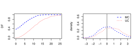
Figure 1: Monte Carlo estimates of limit distributions for estimation of the derivative and the maximum. The left plot gives Monte Carlo estimates of distribution functions of $|\widehat{\varphi}^{\prime}(0)|$ and $|(\widehat{\varphi}^{0})^{\prime}(0)|$. The right plot gives density estimates of $N(\widehat{\varphi})$ and $N(\widehat{\varphi}^{0})$. The number of Monte Carlos used is $10^{3}$, each with sample size $10^{4}$. Here, we sampled from $N(0,1)$ (although this is inconsequential).

5 Simulation results

Software to compute the mode-constrained estimator, and also to implement the likelihood ratio test and corresponding confidence intervals studied in Doss and Wellner (2019), is available in the package logcondens.mode (Doss, 2013a) in R (R Core Team, 2016). Here we illustrate the existence and characterization results on simulated data in Figure 2. There are two columns of four plots. The left column includes the mode-constrained log-concave MLE. The right column includes the $0$-symmetric log-concave MLE. The data points are represented by vertical hash lines along the bottom of each plot. The density, log density, and distribution function are plotted in the top three rows, with the unconstrained log-concave MLE in red and the true (unknown) function in black. On the left the mode-constrained MLE is in blue, and on the right the $0$-symmetric MLE is in blue. The empirical df $\mathbb{F}_{n}$ is plotted in green in the third row. In the last row, we plot $\mathbb{Y}_{n,L}-\widehat{H}_{n,L}^{0}$ (blue) and $\mathbb{Y}_{n,R}-\widehat{H}_{n,R}^{0}$ (purple) to illustrate Theorem 2.4 B (left plot), the corresponding symmetry-constrained process (blue) to illustrate Theorem 2.4 C (right plot), and ${\mathbb{Y}}_{n}-\widehat{H}_{n}$ in red (both plots) to illustrate Theorem 2.4 A. In all the plots, dashed vertical red lines give $S_{n}(\widehat{\varphi}_{n})$ and dashed vertical blue lines give knots of the constrained estimator (which frequently overlap). The solid blue line is the specified mode value for the mode-constrained MLE.

Figure 3 gives plots of $\sqrt{n}(\widehat{G}_{n}^{0}-F_{0})$ (“SC”), $\sqrt{n}(\widehat{F}_{n}^{0}-F_{0})$ (“MC”), $\sqrt{n}(\widehat{F}_{n}-F_{0})$ (“UC”), and $\sqrt{n}(\mathbb{F}_{n}-F_{0})$ (“E”). The left and right plot are each one simulation with sample size $n=200$ and $n=2000$, respectively, from a $N(0,1)$ distribution. The plots show improvements by $\widehat{G}_{n}^{0}$ and $\widehat{F}_{n}^{0}$ over $\widehat{F}_{n}$. The MC and UC lines are indistinguishable when $n=2000$ since one needs to plot locally to the mode $0$ to see differences between $\widehat{F}_{n}^{0}$ and $\widehat{F}_{n}$ when $n$ is large.

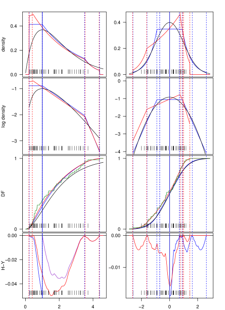
Figure 2: Left: Log-concave MLE and mode-constrained MLE of Gamma with density $xe^{-x}$, $x\geq 0$, with $n=50$ and $m=1$ well-specified. Right: Log-concave MLE and $0$-symmetric MLE of $N(0,1)$ with $n=50$.

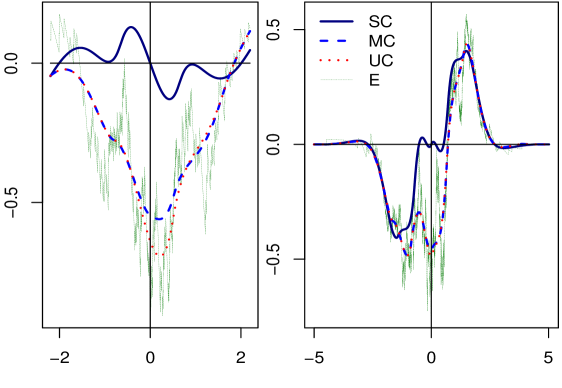
Figure 3: Empirical processes for the symmetry constrained (SC) log-concave MLE, mode constrained (MC) log-concave MLE, unconstrained (UC) log-concave MLE, and empirical (E) distribution. We used a sample of $n=200$ (left) and $n=2000$ (right) from a $N(0,1)$ distribution.

6 Outlook and further problems

Motivated by likelihood ratio test considerations as well as potential uses in several semiparametric settings, we have introduced estimators for a log-concave density known to satisfy a further constraint of either having a known mode or of being symmetric (about $0$). Our estimators are based on the maximum likelihood principle. The constrained MLE’s that we develop are more challenging to compute and to study theoretically than certain naïve estimators discussed in Subsection 2.2, but have much better theoretical behavior. We developed a fast algorithm for computation of the estimators which is made available in the logcondens.mode package for the R programming language. We found that the constrained MLE’s are consistent and indeed we presented the $n^{-2/5}$ rate of convergence, globally and locally (with some proofs given in Doss (2013b)). We found the pointwise asymptotic distribution of the MLE’s, in fact; this necessitated studying and characterizing certain limit processes that govern the limit distributions of the MLE’s. Studying the limit processes in the constrained cases seems to be somewhat more challenging than in the unconstrained case (i.e., than in the case given in Theorem 4.1), because the definitions and characterizing conditions for the constrained limit processes depend on certain knots (of the limit process) in complicated ways. Nonetheless, our proofs of Theorem 4.2 and Theorem 4.4 are different and shorter than the proof of Theorem 4.1; for the latter, Groeneboom, Jongbloed and Wellner (2001a) initially characterized the process on an interval $[-c,c]$ and then through further tightness-type arguments they showed that one can let $c\to\infty$. In the proofs of Theorem 4.2 and Theorem 4.4, we argue directly about a process on $(-\infty,\infty)$, skipping the step of considering the process on $[-c,c]$ and allowing for more direct proofs of the results.

The following are interesting questions beyond those already posed in the introduction that are motivated by the present work.

(a) One motivation for the study of $\widehat{f}_{n}^{0}$ given here has been the likelihood ratio tests and confidence intervals for the mode introduced in Doss and Wellner (2019). But the constrained estimators may be of interest for the study of semiparametric two- and $k-$sample problems with (constrained) log-concave errors. For example suppose that $X_{1},\ldots,X_{m}$ are i.i.d. with $X_{i}\stackrel{{\scriptstyle d}}{{=}}\mu+\varepsilon_{i}$, $i=1,\ldots,m$, while $Y_{1},\ldots,Y_{n}$ are i.i.d. with $Y_{j}\stackrel{{\scriptstyle d}}{{=}}\nu+\delta_{j}$ where $\mu,\nu\in{\mathbb{R}}$ and $\varepsilon_{i},\ \delta_{j}$ are i.i.d. with log-concave density $f$ with mode at $0$. Other variants of this problem might involve constraining $f$ to be log-concave with mean or median at $0$ rather than mode at $0$. Constraining $f$ to be symmetric about its mode of $0$ and log-concave, as in Balabdaoui and Doss (2018), is also of interest.

(b) In Balabdaoui and Doss (2018), a mixture density $g_{0}(x)=\sum_{i=1}^{k}\pi_{i}f_{0}(x-\mu_{i})$ is estimated where $f_{0}$ is constrained to be in ${\cal SLC}_{0}$, $k=2$, $\mu_{1}<\mu_{2}$, and $\pi_{1}=1-\pi_{2}\notin\left\{0,1/2,1\right\}$. Restriction to the case $k=2$ is made for identifiability reasons. Can the asymptotic distribution theory we developed in the present paper be extended to the MLE of $f_{0}$ (and of $g_{0}$) in the semiparametric mixture setting? Extensions to the case $k>2$ could also be possible and would certainly be interesting.

7 Proof sketches and outlines

In this section we give some outlines of the proofs of the results in Section 4. Full proofs are given in Section 8. Here we outline the material in each subsection of Section 8.

Subsection 8.2.1:

The main goal of Subsection 8.2.1 is to show the following proposition.

Proposition 7.1.

Suppose either Assumption 2a holds (at $x_{0}\neq m$) or Assumption 2b holds (at $x_{0}=m$). Let $C>0$ and let $I_{n}=[x_{0}-Cn^{-1/5},x_{0}+Cn^{-1/5}]$. Then

$$\sup_{t\in I_{n}}\left|(\widehat{\varphi}_{n}^{0})^{\prime}(t)-\varphi_{0}^{\prime}(x_{0})\right|=O_{p}(n^{-1/5}),$$ (7.1)

where $(\widehat{\varphi}_{n}^{0})^{\prime}$ denotes either the right or left derivative, and

$$\sup_{t\in I_{n}}\left|\widehat{\varphi}_{n}^{0}(t)-\varphi_{0}(x_{0})-(t-x_{0})\varphi_{0}^{\prime}(x_{0})\right|=O_{p}(n^{-2/5}).$$ (7.2)

We may replace the interval $I_{n}$ by $[\xi_{n}-Cn^{-1/5},\xi_{n}+Cn^{-1/5}]$ for any $\xi_{n}\to m$. Then the random variables implied by the $O_{p}$ upper bounds depend on $C$ but not on $\xi_{n}$.

This proposition is of crucial importance for showing the results in Subsection 4.3 (Theorems 4.7, 4.8, and 4.9). The proof of Proposition 7.1 depends on the following two propositions.

Proposition 7.2.

Let $K=[b,c]$ be a closed interval contained in the interior of the support of $f_{0}\in{\cal LC}_{m}$. Then

$$\sup_{t\in K}|\widehat{\varphi}_{n}^{0}(t)-\varphi_{0}(t)|\rightarrow_{a.s.}0\;\text{ and }\;\sup_{t\in K}|\widehat{f}_{n}^{0}(t)-f_{0}(t)|\rightarrow_{a.s.}0\ \ \ \text{ as }\ \ n\rightarrow\infty.$$

Proposition 7.3.

Suppose that Curvature Assumption 2b holds so $\varphi_{0}^{\prime\prime}(m)<0$.
Let $\tau_{+}^{0}(\xi_{n})$ denote the smallest knot of $\widehat{\varphi}_{n}^{0}$ strictly greater than $\xi_{n}$, and let $\tau_{-}^{0}(\xi_{n})$ denote the largest knot of $\widehat{\varphi}_{n}^{0}$ strictly smaller than $\xi_{n}$. Then for all $\varepsilon>0$ there exists $C^{0}>0$ such that for any random variables $\xi_{n}\rightarrow_{p}m$

$$P(n^{1/5}(\tau_{+}^{0}(\xi_{n})-\tau_{-}^{0}(\xi_{n}))\geq C^{0})\leq\varepsilon$$

for $n\geq N^{0}$ for some $N^{0}$. The integer $N^{0}$ may depend on $\xi_{m}$ but $C^{0}$ does not depend on $\xi_{m}$.

Proposition 7.2 is proved in Doss (2013b). It is needed to show Proposition 7.3, which is needed to prove Proposition 7.1. The proof of Proposition 7.1 depends on Proposition 7.3, finding points of closeness of $\widehat{\varphi}_{n}$ and $\widehat{\varphi}_{n}^{0}$, and properties of convex functions. The full proof of Proposition 7.1 is given in Doss (2013b) (see Corollary 4.2.7 there). Thus the main goal of Subsection 8.2.1 is to prove Proposition 7.3 about the “gap problem” (a term coined in Balabdaoui and Wellner (2007)) for the constrained MLE near $m$. The proof depends on constructing certain (somewhat complicated) classes of perturbation functions which can be related to $\tau_{+}^{0}(\xi_{n})-\tau_{-}^{0}(\xi_{n})$, and then applying an argument pioneered by Kim and Pollard (1990) to these perturbations (see Lemma 8.2).

Subsections 8.2.1 and 8.2.3:

Subsection 8.2.1 is devoted to the proof of Theorem 4.2. The proof proceeds by defining an “objective function”

$$\phi_{a,b}(g)=\frac{1}{2}\int_{a}^{b}g^{2}(t)dt-\int_{a}^{b}g(t)dX(t)$$ (7.3)

for $a<0<b$. Now, $\widehat{\varphi}^{0}$ is not a minimizer of this objective function (which has finite bounds of integration) but we can show that $\widehat{\varphi}^{0}$ behaves in a sense as if it were a minimizer of $\phi_{a,b}$ over a the space of concave functions with mode at $0$. We show that, for certain values $a<0<b$, directional derivatives of $\phi_{a,b}$, $\int_{a}^{b}\Delta(t)(\widehat{\varphi}^{0}(t)dt-dX(t)),$ in the direction of a function $\Delta$ (assumed to be concave with mode at $0$), are either nonnegative or in some cases are zero (see Propositions 8.7 and 8.8 for exact statements). This allows us to argue as follows. We want to show the uniqueness of any $\varphi$ satisfying the characterizing conditions of Theorem 4.2. We assume there exist $\varphi_{1}$ and $\varphi_{2}$ both satisfying the characterizing conditions. We examine $\phi_{a_{2},b_{2}}(\varphi_{1})-\phi_{a_{2},b_{2}}(\varphi_{2})$ and $\phi_{a_{1},b_{1}}(\varphi_{2})-\phi_{a_{1},b_{1}}(\varphi_{1})$ where $a_{i},b_{i}$ are certain knot points for $\varphi_{i}$. By Propositions 8.7 and 8.8, we are able to show that both of these differences are no smaller than $\int_{-n}^{n}(\varphi_{1}(t)-\varphi_{2}(t))^{2}dt>0$ for $n>0$ related to the knot points $a_{i},b_{i}$. On the other hand, after deriving results about the knots $a_{i},b_{i}$ and relating the processes $\varphi_{i}$ to the “observed” process $Y$ (see Lemma 8.9), we are able to show that $\phi_{a_{2},b_{2}}(\varphi_{1})-\phi_{a_{2},b_{2}}(\varphi_{2})$ and $\phi_{a_{1},b_{1}}(\varphi_{2})-\phi_{a_{1},b_{1}}(\varphi_{1})$ are also nonpositive, by using properties of Brownian motion. Thus the difference $\int_{-n}^{n}(\varphi_{1}(t)-\varphi_{2}(t))^{2}dt=0$. By letting $n\to\infty$, we see $\varphi_{1}=\varphi_{2}$ so the proof is complete. The proof is somewhat complicated by the fact that the “knots” of the concave function $\widehat{\varphi}^{0}$ are not separated but rather could be a complicated “Cantor-type” set, as described in Sinai (1992), and so their behavior requires careful analysis. The proof of Theorem 4.4 in Subsection 8.2.3 follows a similar argument.

Subsection 8.2.4:

Theorem 4.5 A about the unconstrained estimator is Theorem 2.1 of Balabdaoui, Rufibach and Wellner (2009). Part B of the theorem is then proved in an identical fashion as that theorem, because for $n$ large enough, in an $n^{-1/5}$ neighborhood of $x_{0}\neq m$, the constrained and unconstrained estimators satisfy the same characterization. Part C then follows from Part B. The main focus of Subsection 8.2.4 is to show Theorem 4.8. Theorem 4.9 follows in a similar fashion. Theorem 4.8 proves Theorem 4.7 B, which we show now. A similar argument shows that Theorem 4.9 proves Theorem 4.7 C.

Proof of Theorem 4.7 B.

Note that, now with $\sigma=1/\sqrt{f_{0}(m)}$ and $a=|\varphi_{0}^{(2)}(m)|/4!$, (4.21) equals

$$\frac{1}{\gamma_{1}\gamma_{2}^{2}}H_{R}^{(2)}(\cdot/\gamma_{2})\equiv\frac{1}{\gamma_{1}\gamma_{2}^{2}}\widehat{\varphi}^{0}(\cdot/\gamma_{2}),$$ (7.4)

where

$$\gamma_{1}=\left(\frac{f_{0}(m)^{4}|\varphi_{0}^{(2)}(m)|^{3}}{(4!)^{3}}\right)^{1/5}=\frac{1}{\sigma}\left(\frac{a}{\sigma}\right)^{3/5},$$ (7.5)

$$\gamma_{2}=\left(\frac{(4!)^{2}}{f_{0}(m)|\varphi_{0}^{(2)}(m)|^{2}}\right)^{1/5}=\left(\frac{\sigma}{a}\right)^{2/5},$$ (7.6)

and we note that

$$\gamma_{1}\gamma_{2}^{3/2}=\sigma^{-1}=\sqrt{f_{0}(m)},\ \ \ \gamma_{1}\gamma_{2}^{4}=a^{-1}=\frac{4!}{|\varphi_{0}^{(2)}(m)|},$$ (7.7)

$$\frac{1}{\gamma_{1}\gamma_{2}^{2}}=C(m,\varphi_{0})\equiv\left(\frac{4!f_{0}(m)^{2}}{|\varphi_{0}^{(2)}(m)|}\right)^{-1/5}.$$ (7.8)

This gives the constant in the limit distribution for $\widehat{\varphi}_{n}^{0}(m)$. For $(\widehat{\varphi}_{n}^{0})^{\prime}(m)$, we see from (7.4) that

$$(\widehat{\varphi}^{0}_{a,\sigma})^{\prime}=_{d}\frac{1}{\gamma_{1}\gamma_{2}^{3}}(\widehat{\varphi}^{0})^{\prime}(\cdot/\gamma_{2}),$$ (7.9)

and $1/\gamma_{1}\gamma_{2}^{3}=D(m,\varphi_{0})$. Thus Theorem 4.7 B follows from Theorem 4.8. ∎

Next we briefly outline the proof of Theorem 4.8. We define two sets of localized processes. We need to define left-side and right-side processes; for ease of exposition, here we only discuss right-side processes. We let $t_{n,b}\equiv m+bn^{-1/5}$. We let $s_{n,R}$ be any knot (sequence) of $\widehat{\varphi}_{n}^{0}$ strictly larger than $m$ satisfying $n^{1/5}(s_{n,R}-m)=O_{p}(1)$. The first set of localized processes is the “$f$-processes” (written in terms of the densities and the empirical distribution):

$$\mathbb{Y}_{n,R}^{f}(b) \equiv n^{4/5}\int_{s_{n,R}}^{t_{n,b}}\left(\int_{s_{n,R}}^{v}(d\mathbb{F}_{n}-f_{0}(m)d\lambda)\right)dv,$$

$$\widehat{H}_{n,R}^{f}(b) \equiv n^{4/5}\int_{s_{n,R}}^{t_{n,b}}\left(\int_{s_{n,R}}^{v}(\widehat{f}_{n}^{0}-f_{0}(m))d\lambda\right)dv+A_{n,R}n^{1/5}(t_{n,b}-s_{n,R}),$$

where $A_{n,R}=n^{3/5}\left(\mathbb{F}_{n,R}(s_{n,R})-\widehat{F}_{n,R}^{0}(s_{n,R})\right)$, and $A_{n,R}n^{1/5}(t_{n,b}-s_{n,R})$ is shown to be asymptotically negligible. These processes are needed because we can show that

$$\mathbb{Y}_{n,R}^{f}(\cdot)\Rightarrow\sqrt{f_{0}(m)}\int_{\nu_{n,R}}^{\cdot}\int_{\nu_{n,R}}^{v}dWdv-f_{0}^{(2)}(m)\int^{\cdot}_{\nu_{n,R}}\int_{\nu_{n,R}}^{v}\frac{u^{2}}{2}dudv$$ (7.10)

where $\nu_{n,R}=n^{1/5}(s_{n,R}-m)$ and $W$ is a standard Brownian motion with $W(0)=0$ (see Lemma 8.17). Furthermore, the characterization from Theorem 2.4 B applies to $\mathbb{Y}_{n,R}^{f}$ and $\widehat{H}_{n,R}^{f}$, so $\mathbb{Y}_{n,R}^{f}(b)-\widehat{H}_{n,R}^{f}(b)\geq 0$ for $b>0$, with equality at certain points (see Lemma 8.18).

On the other hand, the tightness proposition from above, Proposition 7.1, applies to the log-densities. Thus we define the second set of processes, the “$\varphi$-processes”, written in terms of log-densities:

$$\mathbb{Y}_{n,R}^{\varphi}(b) =\frac{\mathbb{Y}_{n,R}^{f}(b)}{f_{0}(m)}-n^{4/5}\int_{s_{n,R}}^{t_{n,b}}\int_{s_{n,R}}^{v}R_{n}^{0}(u)dudv,$$

$$\widehat{H}_{n,R}^{\varphi}(b) =n^{4/5}\int_{s_{n,R}}^{t_{n,b}}\int_{s_{n,R}}^{v}\left(\widehat{\varphi}_{n}^{0}(u)-\varphi_{0}(m)\right)dudv+\frac{A_{n,R}n^{1/5}(t_{n,b}-s_{n,R})}{f_{0}(m)}$$

where $R_{n}^{0}$ is a remainder term. These are related to the $f$-processes by a Taylor expansion (the delta method). One can translate the characterizing inequalities from the $f$-processes to the $\varphi$-processes, to see that $\mathbb{Y}_{n,R}^{\varphi}(b)-\widehat{H}_{n,R}^{\varphi}(b)\geq 0$ for $b\geq 0$ with equality at certain points. By (7.10), $\mathbb{Y}_{n,R}^{\varphi}$ can be shown to converge to a limiting Gaussian process. Furthermore, we can apply Proposition 7.1 and the Arzela-Ascoli theorem (after analyzing various remainder terms) to see that $\widehat{H}_{n,R}^{\varphi}$ is tight (Lemma 8.24).

Finally, we make a subsequence argument using tightness. By tightness, Prohorov’s theorem, and the Skorokhod construction, for any subsequence we can find a further subsubsequence that converges almost surely to a limit process. By using the characterization (Lemma 8.21, and by analysis of various remainder terms), we show that the limit process must satisfy the unique characterizing conditions given by Theorem 4.2. This shows the limit is the same along all subsequences and so the unique process $\widehat{\varphi}^{0}$ given in Theorem 4.2 is the limit, which completes the proof. The argument showing that the characterizing conditions pass from the finite sample processes to the limit process is somewhat complicated by the fact that the integrands in question are defined to begin at random knot points.

Another issue of note is that $(\widehat{\varphi}_{n}^{0})^{\prime}$ is a discontinuous function. We must choose or find an appropriate metric space in which to study its convergence; the metric we choose is the so-called $M_{1}$ Skorokhod metric, which differs from the (perhaps more standard) $J_{1}$ Skorokhod metric (referred to as “the” Skorokhod metric in chapter 12 of Billingsley (1999)). The $J_{1}$ metric unfortunately does not allow multiple jumps to approximate a single jump, whereas the $M_{1}$ metric does. Since we do not have a proof that multiple jumps of $(\widehat{\varphi}_{n}^{0})^{\prime}$ do not approximate a single jump in the limit, we must use the $M_{1}$ metric. See Lemma 8.23 and the preceding text for further discussion.

8 Proofs

8.1 Proofs for Section 2

Proofs of Theorems 2.1 A, 2.2 A, 2.4 A and Corollaries 2.7 A and 2.8 A may be found in Pal, Woodroofe and Meyer (2007), Rufibach (2006), and Dümbgen and Rufibach (2009). Proofs of parts B and C of Corollary 2.7 and part B of Corollary 2.8 follow from the corresponding parts of Theorems 2.2 and 2.4, much as in the unconstrained case, A. It remains to prove parts B and C of Theorems 2.1, 2.2, and 2.4.

In the following proofs, we let ${\cal C}_{n,m}$ denote the (random) class of concave functions with knots at the $Z_{i}$’s and support on $[X_{(1)},X_{(n)}]$, and let ${\cal K}_{n,m}$ denote the class of concave functions $\varphi$ with knots at the $Z_{i}$’s and where $e^{\varphi}$ is a density with support $[X_{(1)},X_{(n)}]$.

Proof of Theorem 2.1.

Proof of Theorem 2.1 B: As in the unconstrained case (Theorem 2.1 of Dümbgen and Rufibach (2009)), it is easy to argue that the solution is piecewise linear with knots at the $Z_{i}$’s, and that $\widehat{\varphi}_{n}^{0}$ is flat either directly to the left of the mode or directly to the right of the mode as long as the mode is not a data point. If the mode is equal to one of the $X_{i}$’s then the proof given by Rufibach (2006) for the unconstrained MLE existence applies directly. Thus assume the mode is not one of the $X_{i}$. Consider a sequence $\left\{v_{j}\right\}$ which has limit coordinates $\gamma=(\gamma_{1},\ldots,\gamma_{N})$ which may be $\pm\infty$. Let $\varphi_{\gamma}$ be the piecewise linear function given by linearly interpolating $\gamma$. Then $\varphi_{\gamma}$ has a flat modal region on $[Z_{i},Z_{j}]$ for some $i<j$. Since $\int e^{\varphi_{\gamma}(x)}dx=1$, we have $\varphi_{\gamma}(m)\leq\log(1/(Z_{j}-Z_{i}))$. Since $m$ is the mode of $e^{\varphi_{\gamma}}$ no coordinate of $\gamma$ is positive infinity, if one of the coordinates is $-\infty$ then $\Psi_{n}(\varphi_{\gamma})=-\infty$. This shows we can consider the continuous function $\Psi_{n}$ on a compact set so it achieves a maximum. The proof that if $\widehat{\psi}_{n}$ maximizes $\Psi_{n}$ over ${\cal C}_{m}$ then $\int e^{\widehat{\psi}_{n}(x)}dx=1$ as well as the proof that $\widehat{\psi}_{n}$ is unique are as in the unconstrained case (Rufibach (2006)).

For Theorem 2.1 C, note that

$$\operatorname*{argmax}_{g\in{\cal SLC}_{0}}\frac{1}{n}\sum_{i=1}^{n}\log g(X_{i})=\operatorname*{argmax}_{g\in{\cal SLC}_{0}}\frac{1}{n}\sum_{i=1}^{n}\log g(|X_{i}|)=\operatorname*{argmax}\frac{1}{n}\sum_{i=1}^{n}\log g(|X_{i}|)$$

where the last argmax is over log-concave functions with mode at $0$ and which integrate to $1/2$ on $[0,\infty)$. ∎

The proof of Theorem 2.2 B is standard. See Doss (2013b). For the proof of Theorem 2.4 B we need to introduce a certain cone $C\subseteq{\mathbb{R}}^{d}$ (defined, e.g., on page 13 of Rockafellar (1970)). We say the cone $C$ is (finitely) generated by a set $\{b_{i}\in C$ : $i=1,\ldots,k<\infty\}$ if for all $c\in C$ we can write $c=\sum_{i=1}^{k}\alpha_{i}b_{i}$ for some nonnegative numbers $\alpha_{i}\geq 0$. Let $(x)_{-}=\min(x,0)$ and $(x)_{+}=\max(x,0)$.

Proposition 8.1.

${\cal C}_{n,m}$ is a convex cone with finite generating set given by

$$\{(x-Z_{i})_{-}\}_{2\leq i\leq k}\,\bigcup\,\{(Z_{i}-x)_{-}\}_{k\leq i\leq N-1}\,\bigcup\{\pm 1\}.$$

Proof.

It is clear that ${\cal C}_{n,m}$ is a cone because concavity and the mode are preserved under positive scaling. For $\varphi\in{\cal C}_{n,m}$, with $\varphi^{\prime}(Z_{i}-)=\sum_{j=i}^{k}a_{j}$ for $i\leq k$, with, $\varphi^{\prime}(Z_{i}+)=\sum_{j=k}^{i}b_{j}$ for $i\geq k$, and with $\varphi(m)=C$, we can write $\varphi(x)=C+\sum_{i=2}^{k}a_{i}(x-Z_{i})_{-}+\sum_{i=k}^{n-1}b_{i}(Z_{i}-x)_{-}$. ∎

Proof of Theorem 2.4.

Proof of Part B: First we assume $\widehat{\varphi}_{n}^{0}$ is the MLE and use (2.5) to show that (2.12) and (2.13) hold. Using the generating functions described in Proposition 8.1 as our $\Delta$ yields equations (2.12) and (2.13) via integration by parts. That is, for $t\leq m$, we choose $\Delta(x)=\left(x-t\right)_{-}$ (which is concave with $m$ as a mode). Then integration by parts yields $-\int_{X_{(1)}}^{t}F(x)dx=\int_{X_{(1)}}^{X_{(n)}}(x-t)_{-}dF(x)$, by Lemma 9.1 B, for $F$ equal to either ${\mathbb{F}}_{n}$ or $\widehat{F}_{n}^{0}$ since $\mathbb{F}_{n}(X_{(1)}-)=\widehat{F}_{n}^{0}(X_{(1)}-)=0$. Thus, by our initial characterization (2.5), we get (2.12). Similarly, for $t\geq m$, let $\Delta(x)=\left(t-x\right)_{-}$; this yields

$${\left(t-X_{(n)}\right){\mathbb{F}}_{n}(X_{(n)})-\int_{t}^{X_{(n)}}{\mathbb{F}}_{n}(x)d(-x)}$$

$$\leq\left(t-X_{(n)}\right)\widehat{F}_{n}^{0}(X_{(n)})-\int_{t}^{X_{(n)}}\widehat{F}_{n}^{0}(x)d(-x),$$

and, recalling that we have already shown $\widehat{F}_{n}^{0}(X_{(n)})=1$, this is equivalent to $\int_{t}^{X_{(n)}}{\mathbb{F}}_{n}(x)dx\leq\int_{t}^{X_{(n)}}\widehat{F}_{n}^{0}(x)dx,$ so we have (2.13). We get equality at some knot points also: set $\Delta(x)=\left(x-b\right)_{+}$ where $b\geq m$ is any RK. Then, by the definition of a RK, $\Delta$ is an allowable perturbation because $\widehat{\varphi}_{n}^{0}(b+)-\widehat{\varphi}_{n}^{0}(b-)>0$ so for some $\delta$ small enough, $\widehat{\varphi}_{n}^{0}+\delta\Delta$ is still concave with mode at $m$. Using this $\Delta$ we get

$${\mathbb{F}}_{n}(X_{(n)})\left(X_{(n)}-b\right)-\int_{b}^{X_{(n)}}{\mathbb{F}}_{n}(x)dx$$

$$=\int_{X_{(1)}}^{X_{(n)}}(x-b)_{+}d{\mathbb{F}}_{n}(x)\leq\int_{X_{(1)}}^{X_{(n)}}(x-b)_{+}d\widehat{F}_{n}^{0}(x)$$

$$=\widehat{F}_{n}^{0}(X_{(n)})\left(X_{(n)}-b\right)-\int_{b}^{X_{(n)}}\widehat{F}_{n}^{0}(x)dx,$$

so that $\int_{b}^{X_{(n)}}{\mathbb{F}}_{n}(x)dx\geq\int_{b}^{X_{(n)}}\widehat{F}_{n}^{0}(x)dx$, and thus for any $b\geq m$ that is a RK we have the inequality both ways, $\int_{b}^{X_{(n)}}{\mathbb{F}}_{n}(x)dx=\int_{b}^{X_{(n)}}\widehat{F}_{n}^{0}(x)dx$. We have thus shown that (2.12) and (2.13) hold with the appropriate equalities.

Now we will show the reverse implication. We assume (2.12) and (2.13) hold and consider $\Delta$ with support $[X_{(1)},X_{(n)}]$ and piecewise linear with knots at the $Z_{i}$. These are all the $\Delta$’s we need to consider, since the rest were ruled out previously by elementary considerations. We also need $\widehat{\varphi}_{n}^{0}+\varepsilon\Delta$ to be concave with mode $m$. Now, we do not know if $m$ will be a NK or a LK or a RK, so we argue by cases. If $m$ is a knot for $\widehat{\varphi}_{n}^{0}$ in one direction, without loss of generality, we can say that $m$ is a RK and we have $\int_{m}^{c}{\mathbb{F}}_{n}(x)dx=\int_{m}^{c}\widehat{F}_{n}^{0}(x)dx$ for any $c>m$ that is also a knot. Recall that we have defined the indices $1=j_{1},\ldots,j_{l^{0}}=N$ so that $Z_{j_{i}}$ are the knots. We write

$$\Delta^{\prime}(r-)=\sum_{i=2}^{l}-C_{i}1_{[Z_{j_{i}-1}<r\leq Z_{j_{i}}]}+\sum_{j=j_{i-1}+1}^{j_{i}}\beta_{j}1_{[Z_{j_{i}-1}<r\leq Z_{j}]}$$ (8.1)

with $\beta_{j}\geq 0$ and all $C_{i}\geq 0$. Since $m$ is a RK, $m$ is not also a LK (otherwise $m$ is simply a knot and $\widehat{\varphi}_{n}^{0}$ coincides with the unconstrained MLE and the characterization of the unconstrained MLE in (Dümbgen and Rufibach, 2009) implies we are done). This forces $C_{p}=0$ (which refers to the interval $(Z_{j_{p}-1},m=Z_{j_{p}}]$). We thus have

$$\int\Delta d{\mathbb{F}}_{n} =\Delta(X_{(n)})-\left[\sum_{i=2}^{l}-C_{i}\int_{Z_{j_{i}-1}}^{Z_{j_{i}}}{\mathbb{F}}_{n}\left(x\right)dx+\sum_{j=j_{i-1}+1}^{j_{i}}\beta_{j}\int_{Z_{j_{i}-1}}^{Z_{j}}{\mathbb{F}}_{n}\left(x\right)dx\right]$$

$$\leq\Delta(X_{(n)})-\left[\sum_{i=2}^{l}-C_{i}\int_{Z_{j_{i}-1}}^{Z_{j_{i}}}\widehat{F}_{n}^{0}\left(x\right)dx+\sum_{j=j_{i-1}+1}^{j_{i}}\beta_{j}\int_{Z_{j_{i}-1}}^{Z_{j}}\widehat{F}_{n}^{0}\left(x\right)dx\right]$$

$$=\int\Delta d\widehat{F}_{n}^{0}$$

as desired, where the inequality follows from noting that $-\beta_{j}\int_{Z_{j_{i}-1}}^{Z_{j}}{\mathbb{F}}_{n}(x)dx\leq-\beta_{j}\int_{Z_{j_{i}-1}}^{Z_{j}}\widehat{F}_{n}^{0}(x)dx$ by assumption and because $\beta_{j}\geq 0$. We also have

$$C_{i}\int_{Z_{j_{i}-1}}^{Z_{j_{i}}}{\mathbb{F}}_{n}\left(x\right)dx=C_{i}\int_{Z_{j_{i}-1}}^{Z_{j_{i}}}\widehat{F}_{n}^{0}\left(x\right)dx$$

for all $i$ except for $i=p$, by the equality-at-knots assumption. However, for $i=p,$ we have $C_{i}=0$. An analogous argument holds for the case where $m$ is an LK and for the case where $m$ is neither an LK nor an RK.

Part C follows as in the proof of Theorem 2.1 C; $\widehat{g}_{n}^{+}$ is the MLE over ${\cal LC}_{0}$ of $|X_{1}|,\ldots,|X_{n}|$. Thus we apply the result of Part B. Note that $0\in S_{n}(\widehat{\psi}_{n}^{0})\cap[0,|X|_{(n)}]$ only if $(\widehat{\psi}_{n}^{0})^{\prime}(0+)<0$ (so that $0$ is a right knot). This is only possible if $0$ is an observed data point. ∎

Proof of Corollary 2.7 B and C follow as in the unconstrained case (Corollary 2.5, Dümbgen and Rufibach (2009)).

8.2 Proofs for local rates of convergence, limit processes, and limit theory

8.2.1 Proofs for local rates of convergence

This section is devoted to showing, Proposition 7.1, stated above, which is needed for proving Theorems 4.8, and 4.9. See 7 for a discussion of the proof of Proposition 7.1, the full details of which are given in Doss (2013b) (Corollary 4.2.7). Our main goal here is to prove Proposition 7.3.

Proof of Proposition 7.3.

We first consider the case $\xi_{n}=m$. For ease of notation and without loss of generality, we assume $m=0$ and abbreviate $\tau_{n,+}^{0}(0)$ by $\tau_{n,+}^{0}$ and $\tau_{n,-}^{0}$ by $\tau_{n,-}^{0}$. We will argue via a family of perturbations which can be separated into subfamilies, depending on whether $0$ is a left-knot (LK), $0$ is a right-knot (RK), or $0$ is not a knot (NK). If $0$ is a one-sided knot (LK or RK), we have different perturbation subfamilies depending on whether $\tau_{n,+}^{0}>-\ \tau_{n,-}^{0}$ or not. We will start with the case in which $0$ is a LK and we construct $\Delta$ that has the two properties

$$\int_{\tau_{n,-}^{0}}^{\tau_{n,+}^{0}}\Delta(t)dt=0,$$ (8.2)

$$\int_{\tau_{n,-}^{0}}^{0}t\Delta(t)dt=0.$$ (8.3)

Whereas in the unconstrained case construction of such an acceptable perturbation function was straightforward (Balabdaoui, Rufibach and Wellner, 2009), in the constrained case, construction of such a $\Delta$ that is an acceptable perturbation (i.e. keeps the mode fixed) is much less straightforward. We consider several cases separately.
Case 1. $\tau_{n,+}^{0}>-\tau_{n,-}^{0}$. In this case we define

$$\Delta_{LK,0}(t)=\begin{cases}\frac{\tau_{n,+}^{0}+m_{2}\cdot(-\frac{\tau_{n,-}^{0}}{4})}{\frac{\tau_{n,-}^{0}}{4}-\tau_{n,-}^{0}}\cdot(t-\tau_{n,-}^{0}),&\,\,\tau_{n,-}^{0}\leq t\leq\frac{\tau_{n,-}^{0}}{4}\\ \tau_{n,+}^{0}+m_{2}\cdot(-t),&\,\,\frac{\tau_{n,-}^{0}}{4}\leq t\leq 0\\ (\tau_{n,+}^{0}-t),&\,\,0\leq t\leq\tau_{n,+}^{0}\\ 0,&\mbox{otherwise,}\end{cases}$$ (8.4)

where

$$m_{2}:=m_{2}(\tau_{n,-}^{0},\tau_{n,+}^{0})=\left(\frac{-9-3\frac{\tau_{n,+}^{0}}{-\tau_{n,-}^{0}}}{1-5\frac{\tau_{n,+}^{0}}{-\tau_{n,-}^{0}}}\right)\left(\frac{\tau_{n,+}^{0}}{-\tau_{n,-}^{0}}\right).$$

This function has integral

$$\frac{(\tau_{n,+}^{0})(5\tau_{n,+}^{0}-\tau_{n,-}^{0})(\tau_{n,+}^{0}-\tau_{n,-}^{0})}{2(5\tau_{n,+}^{0}+\tau_{n,-}^{0})}\equiv M_{LK,case1}(\tau_{n,+}^{0}-\tau_{n,-}^{0}).$$

Case 2: $\tau_{n,+}^{0}<-\tau_{n,-}^{0}$. In this case we define

$$\Delta_{LK,0}(t)=\begin{cases}(t-\tau_{n,-}^{0}),&\,\,\tau_{n,-}^{0}\leq t\leq\frac{\tau_{n,-}^{0}}{2}\\ \frac{\tau_{n,-}^{0}}{2}-\tau_{n,-}^{0}+m_{2}\cdot(\frac{\tau_{n,-}^{0}}{2}-t),&\,\,\frac{\tau_{n,-}^{0}}{2}\leq t\leq 0\\ \ \left(\frac{-\frac{\tau_{n,-}^{0}}{2}+m_{2}\frac{\tau_{n,-}^{0}}{2}}{\tau_{n,+}^{0}}\right)(\tau_{n,+}^{0}-t),&\,\,0\leq t\leq\tau_{n,+}^{0}\\ 0,&\mbox{otherwise,}\end{cases}$$ (8.5)

where

$$m_{2}:=m_{2}(\tau_{n,-}^{0},\tau_{n,+}^{0})=\frac{2\tau_{n,-}^{0}+\tau_{n,+}^{0}}{2\tau_{n,-}^{0}-5\tau_{n,+}^{0}}$$

is defined so that (8.3) holds. This function has integral

$$\frac{-\tau_{n,-}^{0}(3\tau_{n,+}^{0}-\tau_{n,-}^{0})(\tau_{n,+}^{0}-\tau_{n,-}^{0})}{10\tau_{n,+}^{0}-4\tau_{n,-}^{0}}\equiv M_{LK,case2}(\tau_{n,+}^{0}-\tau_{n,-}^{0}).$$

Then we define

$$\Delta_{LK,1}(t)=\Delta_{LK,0}(t)-M_{LK}1_{[\tau_{n,-}^{0},\tau_{n,+}^{0}]}(t),$$ (8.6)

where

$$M_{LK}=\frac{(\tau_{n,+}^{0})(5\tau_{n,+}^{0}-\tau_{n,-}^{0})}{2(5\tau_{n,+}^{0}+\tau_{n,-}^{0})}1_{[\tau_{n,+}^{0}>\tau_{n,-}^{0}]}+\frac{-\tau_{n,-}^{0}(3\tau_{n,+}^{0}-\tau_{n,-}^{0})}{10\tau_{n,+}^{0}-4\tau_{n,-}^{0}}1_{[\tau_{n,+}^{0}\leq\tau_{n,-}^{0}]},$$

is $o_{p}(1)$ by uniform consistency of $\widehat{\varphi}_{n}^{0}$ and is the appropriate shift so that (8.2) holds. Then $\Delta_{LK,0}$ is an acceptable perturbation for $\widehat{\varphi}_{n}^{0}$, since we can have $m_{2}>1$ when $0$ is a LK, and $\Delta_{LK,1}$ has the properties (8.2) and (8.3). We also define $\Delta_{RK,1}$ analogously as $\Delta_{LK,1}$, with analogous constant $M_{RK}$.

Now consider the case in which $0$ is not a knot (NK). In this case, because $(\widehat{\varphi}_{n}^{0})^{\prime}(t)=0$ for all $t\in(\tau_{n,-}^{0},\tau_{n,+}^{0})$, we only need $\Delta$ to have the property

$$\int_{\tau_{n,-}^{0}}^{\tau_{n,+}^{0}}\Delta(t)dt=0.$$ (8.7)

So, if $\tau_{n,+}^{0}>-\tau_{n,-}^{0}$ define

$$\Delta_{NK,0}(t):=\begin{cases}\frac{\tau_{n,+}^{0}}{-\tau_{n,-}^{0}}(t-\tau_{n,-}^{0}),&\mbox{ for }t\in[\tau_{n,-}^{0},0]\\ (\tau_{n,+}^{0}-t),&\mbox{ for }t\in[0,\tau_{n,+}^{0}]\\ 0,&\mbox{ otherwise, }\end{cases}$$ (8.8)

and if $\tau_{n,+}^{0}<-\tau_{n,-}^{0}$, define

$$\Delta_{NK,0}(t):=\begin{cases}(t-\tau_{n,-}^{0}),&\mbox{ for }t\in[\tau_{n,-}^{0},0]\\ \frac{-\tau_{n,-}^{0}}{\tau_{n,+}^{0}}(\tau_{n,+}^{0}-t),&\mbox{ for }t\in[0,\tau_{n,+}^{0}]\\ 0,&\mbox{ otherwise.}\end{cases}$$ (8.9)

Denote $h_{l}=\max(\tau_{n,+}^{0},-\tau_{n,-}^{0})$ and $h_{s}=\min(\tau_{n,+}^{0},-\tau_{n,-}^{0})$. We then compute $\int\Delta_{NK,0}(x)dx=h_{l}(\tau_{n,+}^{0}-\tau_{n,-}^{0})/2$, so set

$$\Delta_{NK,1}(x):=\Delta_{NK,0}(x)-\frac{h_{l}}{2}1_{[\tau_{n,-}^{0},\tau_{n,+}^{0}]}(x),$$ (8.10)

so that (8.7) is satisfied. Let

$$\Delta_{0}(x)=\Delta_{RK,0}(x)1_{[m\text{ is RK}]}+\Delta_{LK,0}(x)1_{[m\text{ is LK}]}+\Delta_{NK,0}(x)1_{[m\text{ is NK}]},$$

$$M_{n}=M_{RK}1_{[m\text{ is RK}]}+M_{LK}1_{[m\text{ is LK}]}+h_{l}1_{[m\text{ is NK}]},$$

and let

$$\begin{split}\Delta_{1}(x)&=\Delta_{RK,1}(x)1_{[m\text{ is RK}]}+\Delta_{LK,1}(x)1_{[m\text{ is LK}]}+\Delta_{NK,1}(x)1_{[m\text{ is NK}]}\\ &=\Delta_{0}(x)-M_{n}.\end{split}$$ (8.11)

Note that $M_{n}$ is $o_{p}(1)$ by uniform consistency in a neighborhood of $m$. By the characterization Theorem 2.2B and Corollary 2.7, we see that

$$\int\Delta_{1}d({\mathbb{F}}_{n}-F_{0}) = \int\Delta_{1}d({\mathbb{F}}_{n}-\widehat{F}_{n}^{0})+\int\Delta_{1}d(\widehat{F}_{n}^{0}-F_{0})$$ (8.12)

$$= \int\Delta_{0}d({\mathbb{F}}_{n}-\widehat{F}_{n}^{0})-M_{n}\int_{\tau_{n,-}^{0}}^{\tau_{n,+}^{0}}d({\mathbb{F}}_{n}-\widehat{F}_{n}^{0})+\int\Delta_{1}d(\widehat{F}_{n}^{0}-F_{0})$$

$$\leq M_{n}\bigg{|}\int_{\tau_{n,-}^{0}}^{\tau_{n,+}^{0}}d({\mathbb{F}}_{n}-\widehat{F}_{n}^{0})\bigg{|}+\int\Delta_{1}(x)(\widehat{f}_{n}^{0}-f_{0})(x)dx$$

$$\leq \frac{2M_{n}}{n}+\int\Delta_{1}(x)(\widehat{f}_{n}^{0}-f_{0})(x)dx.$$

Then Lemma 8.2 yields

$$\left|\int\Delta_{1}d({\mathbb{F}}_{n}-F_{0})\right|\leq O_{p}(n^{-4/5})+\frac{K}{2}h_{l}^{4},$$ (8.13)

$$\int\Delta_{1}(x)(\widehat{f}_{n}^{0}-f_{0})(x)dx\leq-Kh_{l}^{4}+o_{p}(h_{l}^{4}),$$

for some $K>0$ and where we picked $\varepsilon$ from Lemma 8.2 to be $K/2$. So, by rearranging (8.12), we have

$$K(1+o_{p}(1))h_{l}^{4} \leq -\int\Delta_{1}(x)(\widehat{f}_{n}-f_{0})(x)dx$$

$$\leq \frac{2M_{n}}{n}-\int\Delta_{1}d({\mathbb{F}}_{n}-F_{0})\leq\frac{2M_{n}}{n}+\bigg{|}\int\Delta_{1}d({\mathbb{F}}_{n}-F_{0})\bigg{|}$$

$$\leq O_{p}(n^{-4/5})+\frac{K}{2}h_{l}^{4},$$

and hence

$$(K/2+o_{p}(1))h_{l}^{4})\leq O_{p}(n^{-4/5})$$

which yields $0\leq h_{l}=O_{p}(n^{-1/5})$. Since $\tau_{n,+}^{0}$ and $-\tau_{n,-}^{0}$ are both bounded by $h_{l}$, we are done for the case $\xi_{n}=m$.

Extending to the case where $\xi_{n}\to m$ rather than being fixed and equal to $m$ follows from considering the event $m\in[\tau_{n,-}^{0}(\xi_{n}),\tau_{n,+}^{0}(\xi_{n})]$ and its complement separately, and then by showing on the event $m\notin[\tau_{n,-}^{0}(\xi_{n}),\tau_{n,+}^{0}(\xi_{n})]$ that $\tau_{n,+}^{0}(\xi_{n})-\tau_{n,-}^{0}(\xi_{n})=O_{p}(n^{-1/5})$. This is straightforward. ∎

The following lemmas were used.

Lemma 8.2.

We continue with the setup of Proposition 7.3. That is, we define $h_{l}=\max(\tau_{n,+}^{0}-m,m-\tau_{n,-}^{0})$, $h_{s}=\min(\tau_{n,+}^{0}-m,m-\tau_{n,-}^{0})$ and $\Delta_{1}$ as in (8.11). Then for all $\varepsilon>0$,

$$\left|\int\Delta_{1}d({\mathbb{F}}_{n}-F_{0})\right|\leq\varepsilon h_{l}^{4}+O_{p}(n^{-4/5})$$ (8.14)

and

$$\int\Delta_{1}(x)(\widehat{f}_{n}^{0}-f_{0})(x)dx\leq-\frac{f_{0}(0)|\varphi_{0}^{\prime\prime}(0)|}{2}Kh_{l}^{4}+o_{p}(h_{l}^{4}),$$ (8.15)

where $K>0$ is from Lemma 8.3, and does not depend on $f_{0}$.

Proof.

We examine $\int\Delta_{1}(x)(\widehat{f}_{n}^{0}-f_{0})(x)dx$ by repeated Taylor expansions, where we let $\Delta_{1}$ be $\Delta_{LK,1}$ or $\Delta_{NK,1}$, and we will expand at $m$, which we again take to be $0$, without loss of generality. Write $(\widehat{f}_{n}^{0}-f_{0})=f_{0}((\widehat{f}_{n}^{0}/f_{0})-1)=f_{0}(\exp\{\widehat{\varphi}_{n}^{0}-\varphi_{0}\}-1)$. Then write $d_{n}=\widehat{\varphi}_{n}^{0}-\varphi_{0}$ so we can expand

$$\exp(d_{n}(t))-1 = \sum_{i=1}^{1}\frac{d_{n}(t)^{i}}{i!}+e^{\xi_{1,n,t}}\frac{d_{n}(t)^{2}}{2!},$$

$$f_{0}(t) = \sum_{i=0}^{1}\frac{f_{0}^{(i)}(0)t^{i}}{i!}+\frac{f_{0}^{(2)}(\xi_{2,n,t})t^{2}}{2!}$$

for $t\in[\tau_{n,-}^{0},\tau_{n,+}^{0}]$, where $\xi_{1,n,t}$ is between $0$ and $d_{n}(t)$ and $\xi_{2,n,t}$ is between $0$ and $t$. So, writing $\|\cdot\|_{\infty}$ as the uniform norm over $[\tau_{n,-}^{0},\tau_{n,,+}^{0}]$, we can see that $f_{0}(t)(e^{d_{n}(t)}-1)$ equals

$$\left(\sum_{i=0}^{1}\frac{(f_{0})^{(i)}(0)t^{i}}{i!}+\frac{(f_{0})^{(2)}(\xi_{2,n,t})t^{2}}{2!}\right)\left(\sum_{i=1}^{1}\frac{d_{n}(t)^{i}}{i!}+e^{\xi_{1,n,t}}\frac{d_{n}(t)^{2}}{2!}\right)$$

$$=f_{0}(0)d_{n}(t)+o_{p}(\|d_{n}(t)\|_{\infty})$$

since $f_{0}(0)>0,$ $f_{0}^{(i)}$ is continuous and thus bounded on a neighborhood of $0$ for $i\in\{0,1,2\}$, and, by uniform consistency, $d_{n}(t)^{i}$ and $t^{i}$ both go to $0$ uniformly in a neighborhood of $0$. Then we examine

$$\int_{\tau_{n,-}^{0}}^{\tau_{n,+}^{0}}\Delta_{1}(t)d_{n}(t)dt=\sum_{i=0}^{1}\frac{d_{n}^{(i)}(0)}{i!}\int_{\tau_{n,-}^{0}}^{\tau_{n,+}^{0}}t^{i}\Delta_{1}(t)dt+\int_{\tau_{n,-}^{0}}^{\tau_{n,+}^{0}}\frac{d_{n}^{(2)}(\xi_{3,n,t})}{2!}t^{2}\Delta_{1}(t)dt$$

where $\xi_{3,n,t}\in[\tau_{n,-}^{0},\tau_{n,+}^{0}]$. Note that $d_{n}^{(2)}(t)=-\varphi_{0}^{(2)}(t)$, and that since $d_{n}^{(2)}$ is continuous at $0$ we can write $d_{n}^{(2)}(\xi_{3,n,t})=d_{n}^{(2)}(0)+\varepsilon_{n}(t)$ where $\|\varepsilon_{n}(t)\|_{\infty}\rightarrow_{p}0$ since $\tau_{n,+}^{0}-\tau_{n,-}^{0}\rightarrow_{p}0$. Now we consider the different possible forms $\Delta_{1}$ may take.

If $0$ is NK, then $(\widehat{\varphi}_{n}^{0})^{(2)}(0)=0=\varphi_{0}^{\prime}(0)$, so

$$\int_{\tau_{n,-}^{0}}^{\tau_{n,+}^{0}}\Delta_{NK,1}(t)d_{n}(t)dt$$ (8.16)

$$= \sum_{i=0}^{2}\frac{d_{n}^{(i)}(0)}{i!}\int_{\tau_{n,-}^{0}}^{\tau_{n,+}^{0}}t^{i}\Delta_{NK,1}(t)dt+\int_{\tau_{n,-}^{0}}^{\tau_{n,+}^{0}}\frac{\varepsilon_{n}(t)}{2!}t^{2}\Delta_{NK,1}(t)dt$$

$$= -\frac{\varphi_{0}^{(2)}(0)}{2!}\int_{\tau_{n,-}^{0}}^{\tau_{n,+}^{0}}t^{2}\Delta_{NK,1}(t)dt+\ \int_{\tau_{n,-}^{0}}^{\tau_{n,+}^{0}}\frac{\varepsilon_{n}(t)}{2!}t^{2}\Delta_{NK,1}(t)dt.$$

Now we show that we get the same expansion if $0$ is a LK. Note that for $t\in[0,\tau_{n,+}^{0}],$ $\widehat{\varphi}_{n}^{0}(t)=\widehat{\varphi}_{n}^{0}(0)$ and for $t\in[\tau_{n,-}^{0},0]$, $\widehat{\varphi}_{n}^{0}(t)=\widehat{\varphi}_{n}^{0}(0)+(\widehat{\varphi}_{n}^{0})^{\prime}(0-)t$. Thus

$$\int_{\tau_{n,-}^{0}}^{\tau_{n,+}^{0}}\Delta_{LK,1}(t)\widehat{\varphi}_{n}^{0}(t)dt =\int_{\tau_{n,-}^{0}}^{0}\Delta_{LK,1}(t)\widehat{\varphi}_{n}^{0}(t)dt+\int_{0}^{\tau_{n,+}^{0}}\Delta_{LK,1}(t)\widehat{\varphi}_{n}^{0}(t)dt$$

$$=\widehat{\varphi}_{n}^{0}(0)\int_{\tau_{n,-}^{0}}^{0}\Delta_{LK,1}(t)dt+(\widehat{\varphi}_{n}^{0})^{\prime}(0-)\int_{\tau_{n,-}^{0}}^{0}t\Delta_{LK,1}(t)dt$$

$$\ \ +\ \widehat{\varphi}_{n}^{0}(0)\int_{0}^{\tau_{n,+}^{0}}\Delta_{LK,1}(t)dt$$

$$=0.$$

Hence,

$$\int_{\tau_{n,-}^{0}}^{\tau_{n,+}^{0}}\Delta_{LK,1}(t)d_{n}(t)dt$$ (8.17)

$$= \int_{\tau_{n,-}^{0}}^{\tau_{n,+}^{0}}\Delta_{LK,1}(t)\widehat{\varphi}_{n}^{0}(t)dt-\int_{\tau_{n,-}^{0}}^{\tau_{n,+}^{0}}\Delta_{LK,1}(t)\varphi_{0}(t)dt$$

$$= -\int_{\tau_{n,-}^{0}}^{\tau_{n,+}^{0}}\Delta_{LK,1}(t)\varphi_{0}(t)dt$$

$$= -\sum_{i=0}^{2}\frac{\varphi_{0}^{(i)}(0)}{i!}\int_{\tau_{n,-}^{0}}^{\tau_{n,+}^{0}}t^{i}\Delta_{LK,1}(t)dt+\int_{\tau_{n,-}^{0}}^{\tau_{n,+}^{0}}\frac{\varepsilon_{n}(t)}{2!}t^{2}\Delta_{LK,1}(t)dt$$

$$= -\frac{\varphi_{0}^{(2)}(0)}{2!}\int_{\tau_{n,-}^{0}}^{\tau_{n,+}^{0}}t^{2}\Delta_{LK,1}(t)dt+\int_{\tau_{n,-}^{0}}^{\tau_{n,+}^{0}}\frac{\varepsilon_{n}(t)}{2!}t^{2}\Delta_{LK,1}(t)dt.$$

Since an analogous statement holds for $\Delta_{RK,1}$, we have shown

$$\int_{\tau_{n,-}^{0}}^{\tau_{n,+}^{0}}\Delta_{1}(t)d_{n}(t)dt = -\frac{\varphi_{0}^{(2)}(0)}{2!}\int_{\tau_{n,-}^{0}}^{\tau_{n,+}^{0}}t^{2}\Delta_{1}(t)dt+\int_{\tau_{n,-}^{0}}^{\tau_{n,+}^{0}}\frac{\varepsilon_{n}(t)}{2!}t^{2}\Delta_{1}(t)dt$$

where $\|\varepsilon_{n}\|_{\infty}\rightarrow_{p}0$. Thus

$$\int\Delta_{1}(x)(\widehat{f}_{n}^{0}-f_{0})(x)dx = f_{0}(0)(1+o_{p}(1))\int\Delta_{1}(t)d_{n}(t)$$

$$= f_{0}(0)(1+o_{p}(1))^{2}\frac{-\varphi_{0}{(2)}(0)}{2!}\int_{\tau_{n,-}^{0}}^{\tau_{n,+}^{0}}t^{2}\Delta_{1}(t)dt.$$

Lemma 8.3 shows that

$$\int_{\tau_{n,-}^{0}}^{\tau_{n,+}^{0}}t^{2}\Delta_{1}(t)dt\leq-Kh_{l}^{4}\$$ (8.18)

which yields (8.15), our desired conclusion:

$$\int_{\tau_{n,-}^{0}}^{\tau_{n,+}^{0}}\Delta_{1}(t)\left(\widehat{f}_{n}^{0}-f_{0}\right)(t)dt \leq -\frac{f_{0}(0)|\varphi_{0}^{(2)}(0)|}{2}Kh_{l}^{4}+o(h_{l}^{4}).$$

Now we show (8.14). First for a fixed $\delta>0$, we know that $\tau_{n,+}^{0}$ and $\tau_{n,-}^{0}$ will be in $[-\delta,\delta]$ eventually, with high probability. Now we consider three families of functions, analogous to $\Delta_{LK,1}$, $\Delta_{RK,1}$, and $\Delta_{NK,1}$, respectively. Define $\Delta_{LK,1,b,c}$ by replacing $\tau_{n,-}^{0}$ with $b$ and $\tau_{n,+}^{0}$ with $c$ in (8.6). Define $\Delta_{NK,1,b,c}$ by replacing $\tau_{n,-}^{0}$ with $b$ and $\tau_{n,+}^{0}$ with $c$ in (8.10). Define $\mathcal{F}_{LK,b,R}:=\{\Delta_{LK,b,y}|b<a<y,\mbox{ }0\leq y-b\leq R\}$ and $\mathcal{F}_{NK,b,R}:=\{\Delta_{NK,b,y}|b<a<y,\mbox{ }0\leq y-b\leq R\}$ for $R>-b$. Define $\mathcal{F}_{RK,b,R}$ analogously to $\mathcal{F}_{LK,b,R}$. Let $\mathcal{F}=\mathcal{F}_{LK,b,R}\cup\mathcal{F}_{RK,b,R}\cup\mathcal{F}_{NK,b,R}$, and note that $\mathcal{F}$ is VC-class with VC-index of $4$. Thus Theorem 2.6.7 on page 141 of van der Vaart and Wellner (1996) shows that the entropy bound condition in Lemma A.1 on page 2560 of Balabdaoui and Wellner (2007) holds for $\mathcal{F}$. Then the function $F_{b,R}(x)$, defined to be constant equal to $(7/4)R$ on $[b,b+R]$ and $0$ otherwise, is an envelope for $\mathcal{F}$. That $F_{b,R}$ is an envelope is immediate for $\Delta\in\mathcal{F}_{NK,b,R}$ and for the setting where $\tau_{n,+}^{0}<-\tau_{n,-}^{0}$ and $\Delta\in\mathcal{F}_{LK,b,R}$ (and analogously when $\tau_{n,+}^{0}>-\tau_{n,-}^{0}$ and $\Delta\in\mathcal{F}_{RK,b,R}$). (For $\Delta\in\mathcal{F}_{NK,b,R}$, the longer interval has slope $\pm 1$ and the other interval has opposite sign slope. For the case $\tau_{n,+}^{0}<-\tau_{n,-}^{0}$ and $\Delta\in\mathcal{F}_{LK,b,R}$, the interval $[\tau_{n,-}^{0},\tau_{n,-}^{0}/2]$ has slope $1$ and the slope on the rest is opposite sign (and analogously for $\mathcal{F}_{RK,b,R}$).) For the case $\tau_{n,+}^{0}\geq-\tau_{n,-}^{0}$ and $\Delta\in\mathcal{F}_{LK,b,R}$, we need only note

$$0\leq m_{2}=\frac{\tau_{n,+}^{0}}{-\tau_{n,-}^{0}}\left(\frac{-9-3\frac{\tau_{n,+}^{0}}{-\tau_{n,-}^{0}}}{1-5\frac{\tau_{n,+}^{0}}{-\tau_{n,-}^{0}}}\right)\leq 3,$$

so that $(-\tau_{n,-}^{0}/4)m_{2}\leq(3/4)\tau_{n,+}^{0}$. Next, we compute the integral of the envelope squared

$$EF_{b,R}^{2}(X) = \int_{b}^{b+R}R^{2}f_{0}(x)dx\leq\|f_{0}\|_{\infty}R^{3},$$

where $\|f_{0}\|_{\infty}$ is the supremum over ${\mathbb{R}}$ of the (log-concave) density $f_{0}$, and is thus universal across $b$ and $R$. Thus, we can conclude from Lemma A.1 on page 2560 of Balabdaoui and Wellner (2007) that for $\varepsilon>0$ and with $s=2$ and $d=2$,

$$\left|\int\Delta_{1}d({\mathbb{F}}_{n}-F_{0})\right| \leq \varepsilon(\tau_{n,+}^{0}-\tau_{n,-}^{0})^{4}+O_{p}(n^{-4/5}),$$

$$\leq \varepsilon 2^{4}h_{l}^{4}+O_{p}(n^{-4/5})$$

as desired. ∎

Lemma 8.3.

For $h_{l}=\max(\tau_{n,+}^{0}-m,m-\tau_{n,-}^{0})$, $h_{s}=\min(\tau_{n,+}^{0}-m,m-\tau_{n,-}^{0})$ and $\Delta_{1}$ defined by (8.11), we have

$$\int\Delta_{1}(t)(t-m)^{2}dt \leq -Kh_{l}^{4},$$

for some $K>0$.

Proof.

First, we consider $\Delta_{LK,1}$, assume without loss of generality that $m=0$, and assume $\tau_{n,+}^{0}>-\tau_{n,-}^{0}$. Direct computation shows

$$\int_{\tau_{n,-}^{0}}^{\tau_{n,+}^{0}}t\Delta_{LK,1}(t)dt =-\frac{5}{12}\left(\frac{(\tau_{n,+}^{0}-\tau_{n,-}^{0})(\tau_{n,+}^{0})^{3}}{5\tau_{n,+}^{0}+\tau_{n,-}^{0}}\right)\leq-\frac{5}{12}\left(\frac{(\tau_{n,+}^{0}-\tau_{n,-}^{0})(\tau_{n,+}^{0})^{3}}{5(\tau_{n,+}^{0})}\right)$$

and this is bounded above by

$$-\frac{5}{12}\frac{(\tau_{n,+}^{0})^{4}}{5\tau_{n,+}^{0}}=-\frac{(\tau_{n,+}^{0})^{3}}{12}=-\frac{h_{l}^{3}}{12},$$

since $\tau_{n,+}^{0}>-\tau_{n,-}^{0}$.

We break $\int_{\tau_{n,-}^{0}}^{\tau_{n,+}^{0}}t^{2}\Delta_{LK,1}(t)dt$ into two pieces. First we see

$$\int_{\tau_{n,-}^{0}}^{0}t^{2}\Delta_{LK,1}(t)dt = \frac{-3(\tau_{n,-}^{0})^{4}\tau_{n,+}^{0}-19(-(\tau_{n,-}^{0}))^{3}(\tau_{n,+}^{0})^{2}}{96(5\tau_{n,+}^{0}+\tau_{n,-}^{0})}<0.$$

Next we see that

$$\int_{0}^{\tau_{n,+}^{0}}t^{2}\Delta_{LK,1}(t)dt = \frac{-3(-\tau_{n,-}^{0})(\tau_{n,+}^{0})^{4}-5(\tau_{n,+}^{0})^{5}}{12(5\tau_{n,+}^{0}+\tau_{n,-}^{0})}$$

$$\leq -\frac{3(-\tau_{n,-}^{0})(\tau_{n,+}^{0})^{4}+5(\tau_{n,+}^{0})^{5}}{12\cdot 5(\tau_{n,+}^{0})}\leq-\frac{(\tau_{n,+}^{0})^{4}}{12}.$$

Thus,

$$\int_{\tau_{n,-}^{0}}^{\tau_{n,+}^{0}}t^{2}\Delta_{LK,1}(t)dt\leq-\frac{(\tau_{n,+}^{0})^{4}}{12}=-\frac{h_{l}^{4}}{12},$$

as desired.

Now we consider $\Delta_{LK,1}$ when $\tau_{n,+}^{0}<-\tau_{n,-}^{0}$, and again split the computation into two pieces. First we see

$$\int_{0}^{\tau_{n,+}^{0}}t^{2}\Delta_{LK,1}(t)dt = -\frac{2(\tau_{n,-}^{0})^{2}(\tau_{n,+}^{0})^{3}-3(\tau_{n,+}^{0})^{5}}{12(5\tau_{n,+}^{0}-2\tau_{n,-}^{0})}.$$

Next we find that

$$\int_{\tau_{n,-}^{0}}^{a}t^{2}\Delta_{LK,1}(t)dt = -\frac{(-\tau_{n,-}^{0})^{5}+5(\tau_{n,-}^{0})^{4}\tau_{n,+}^{0}}{48(5\tau_{n,+}^{0}-2\tau_{n,-}^{0})}$$

so that

$$\int_{\tau_{n,-}^{0}}^{\tau_{n,+}^{0}}t^{2}\Delta_{LK,1}(t)dt = \frac{(\tau_{n,-}^{0})^{5}-5(\tau_{n,-}^{0})^{4}\tau_{n,+}^{0}-8(\tau_{n,-}^{0})^{3}(\tau_{n,+})^{3}+12(\tau_{n,+}^{0})^{5}}{48(5\tau_{n,+}^{0}-2\tau_{n,-}^{0})}$$ (8.19)

$$\leq -\frac{(-\tau_{n,-}^{0})^{4}}{48\cdot 7}$$

and it remains only to prove the last inequality. To do this, let $a\equiv\tau_{n,-}^{0}<0<\tau_{n,+}^{0}\equiv b$ where $-a\geq b$. Thus we want to show that

$$K(a,b)=-5a^{5}+30a^{4}b+56a^{2}b^{3}-84b^{5}\geq 0$$

for all $a<0<b$ with $-a\geq b$. But this holds if and only if $J(v,c)\equiv K(-v,cv)\geq 0$ holds for all $v\geq 0$ and $0\leq c\leq 1$. But

$$J(v,c)=K(-v,cv)\geq v^{5}(5c^{5}+30c^{5}+56c^{5}-84c^{5}) =v^{5}c^{5}\cdot 7\geq 0.$$

Thus (8.19) holds.

Identical calculations hold for $\Delta_{RK,1}$. Now we examine $\Delta_{NK,1}$. Direct computation shows

$$\int_{\tau_{n,-}^{0}}^{\tau_{n,+}^{0}}t^{2}\Delta_{NK,1}(t)dt=-\frac{1}{12}(h_{s}^{3}h_{l}+h_{l}^{4})\leq-\frac{1}{12}h_{l}^{4}.$$

∎

8.2.2 Proofs for mode-constrained limit process

This entire section is devoted to the proof of Theorem 4.2, and thus throughout this section we take the definitions and assumptions as given in that theorem.

Proof of Lemma 4.3.

If $0\in\widehat{S}^{0}$ then one of $\tau_{+}^{0}$ or $\tau_{-}^{0}$ is $0$, because then $(\widehat{\varphi}^{0})^{(2)}$ is not constant-equal-to-$0$ on any open neighborhood of $0$; if it is not constant-equal-to-$0$ on $[0,\delta)$ for any $0<\delta$ then $(\widehat{\varphi}^{0})^{\prime}$ is also not constant on $[0,\delta)$, so since $0\geq(\widehat{\varphi}^{0})^{\prime}(0+)$, we have $(\widehat{\varphi}^{0})^{\prime}(\delta+)<0$ for all $\delta>0$, i.e. $\tau_{+}^{0}=0$ (of course $\tau_{+}^{0}\geq 0$ since $0$ is the mode of $\widehat{\varphi}^{0}$). Similarly, if $(\widehat{\varphi}^{0})^{(2)}$ is not $0$ on any neighborhood below $0$, then $\tau_{-}^{0}=0$.

Now, if $0\notin\widehat{S}^{0}$ then $\tau_{-}^{0}=\sup\widehat{S}^{0}\cap(-\infty,0]$ and $\tau_{+}^{0}=\inf\widehat{S}^{0}\cap[0,\infty)$. If $0\in\widehat{S}^{0}$ then we have shown that one of $\tau^{0}_{\pm}$ equals $0$. Thus, in either case, it is clear that $(\widehat{\varphi}^{0})^{(2)}(t\pm)=0$ for $0\leq t<\tau_{+}^{0}$ and for $\tau_{-}^{0}<t\leq 0$. Thus, regardless of whether $0\in\widehat{S}^{0}$, $(\widehat{\varphi}^{0})^{(2)}$ and so $(\widehat{\varphi}^{0})^{\prime}$ are constant and equal to $0$ on $(\tau_{-}^{0},\tau_{+}^{0})$, i.e. (4.11) holds (and so $(\tau_{-}^{0},\tau_{+}^{0})$ is the modal interval of $\widehat{\varphi}^{0}$). ∎

The next lemma gives the sense in which $\widehat{\varphi}^{0}$ is piecewise affine.

Lemma 8.4.

Assume that $H_{L},H_{R},$ and $\widehat{\varphi}^{0}$ are as in Theorem 4.2. Define

$$S_{L} =\{t\leq 0:H_{L}(t)=Y_{L}(t),H_{L}^{\prime}(t)=Y_{L}^{\prime}(t)\},$$

$$S_{R} =\{t\geq 0:H_{R}(t)=Y_{R}(t),H_{R}^{\prime}(t)=Y_{R}^{\prime}(t)\},$$

$$\mbox{ and }S^{0} =S_{L}\cup S_{R}\cup\{0\}.$$ (8.20)

Then $(\widehat{\varphi}^{0})^{\prime}$ is a monotonically nonincreasing function and the ‘bend points’ of $\widehat{\varphi}^{0}$, $\widehat{S}^{0}$, defined in (4.2), satisfy $\widehat{S}^{0}\subset S^{0}$. Additionally, with probability $1$ the following statements hold. The sets $S_{L},S_{R},$ and $S^{0}$ are all closed and have Lebesgue measure $0$. For any fixed $t\neq 0$, $t\notin S^{0}$ and so $(H^{0})^{(3)}(t)$ is well-defined.

The lemma says that for any knot $\tau\leq\tau_{+}^{0}$, if $\tau<0$ then $\tau\in S_{L}$. Similarly if $\tau\geq\tau_{-}^{0}$ and $\tau>0$ then $\tau\in S_{R}$. It is possible but not guaranteed that $0$ is a knot and lies in either $S_{L}$ or $S_{R}$.

Proof.

By Theorem 4.2, displays (4.8) and (4.9), $H^{0}-Y^{0}\leq 0$, which allows us to conclude

$$\begin{split}\left\{t<0:H_{L}(t)=Y_{L}(t)\right\}&=\left\{t<0:H_{L}(t)=Y_{L}(t),H_{L}^{\prime}(t)=Y_{L}^{\prime}(t)\right\},\\ \left\{t>0:H_{R}(t)=Y_{R}(t)\right\}&=\left\{t>0:H_{R}(t)=Y_{R}(t),H_{R}^{\prime}(t)=Y_{R}^{\prime}(t)\right\};\end{split}$$ (8.21)

the first line follows since $H_{L}-Y_{L}$ is differentiable on $(-\infty,0)$, and a differentiable function has derivative $0$ at a local maximum (see, e.g., Dieudonné (1969), page 153, Problem 3, part (a)). The same argument applies to the second line of (8.21).

Now, the following argument holds with probability $1$ and for any fixed $c>0$. On $[0,c]$, $H_{R}$ has a bounded second derivative, so that there exists a constant $a>0$ such that $\tilde{H}_{R}(t):=H_{R}(t)+at^{2}$ is convex on $[0,c]$. Let $\tilde{Y}_{R}(t):=Y_{R}(t)+at^{2}.$ Now, $Y_{R}+A=Y$ for an affine function $A$ and where $Y(t)=\int_{0}^{t}\int_{0}^{u}dX(z)du$. Let $\tilde{Y}(t)=Y(t)+at^{2}=\tilde{Y}_{R}(t)+A(t)$ so that

$$\begin{split}\{x\in[0,c]:H_{R}(x)=Y_{R}(x)\}&=\{x\in[0,c]:\tilde{H}_{R}(x)+A(x)=\tilde{Y}_{R}(x)+A(x)\}\\ &=\{x\in[0,c]:\tilde{H}_{R}(x)+A(x)=\tilde{Y}(x)\}\end{split}$$ (8.22)

We also have $\tilde{H}_{R}+A\leq\tilde{Y}_{R}+A=\tilde{Y}$ by (4.9), so that, letting $M_{\tilde{Y}}$ be the greatest convex minorant of $\tilde{Y}$ on $[0,c]$, we have $\tilde{H}_{R}+A\leq M_{\tilde{Y}}\leq\tilde{Y}$, since $\tilde{H}_{R}+A$ is convex and below $\tilde{Y}$.

Let $T=\left\{x\in[0,c]:M_{\tilde{Y}}(x)=\tilde{Y}(x)\right\}$. By the proof of Corollary 2.1 of Groeneboom, Jongbloed and Wellner (2001a) (see also Definition 1 and Theorem 1 of Sinai (1992)), $T$ is a (Cantor-type) set which has Lebesgue measure $0$; (8.22) is contained in $T$, and thus (by (8.21) and) by letting $c\to\infty$, we see that $S_{R}$ is contained in a set which has Lebesgue measure $0$. Finally, $S_{R}$ is closed because $H_{R}-Y_{R}$ and $(H_{R}-Y_{R})^{\prime}$ are both continuous functions. By an analogous argument, we can conclude that $S_{L}$ is closed and has Lebesgue measure $0$ and thus also $S^{0}$ is closed and has Lebesgue measure $0$. By (4.10),

$$\int_{\{t\in(-\infty,\tau_{-}^{0}]:H_{L}(t)\neq Y_{L}(t)\}}d(\widehat{\varphi}^{0})^{\prime}(t)=0=\int_{\{t\in[\tau_{+}^{0},\infty):H_{R}(t)\neq Y_{R}(t)\}}d(\widehat{\varphi}^{0})^{\prime}(t),$$ (8.23)

(regardless of whether one of $\tau_{+}^{0}$ or $\tau_{-}^{0}$ is $0$ or not).

Thus we now conclude that $\widehat{S}^{0}\subset S^{0}$ as follows. If $\tau$ is an element of the set $\widehat{S}^{0}$ then for any $\varepsilon>0$ $(\widehat{\varphi}^{0})^{\prime}(\tau-\varepsilon,\tau+\varepsilon)<0$ (here $(\widehat{\varphi}^{0})^{\prime}$ refers to the signed measure corresponding to $(\widehat{\varphi}^{0})^{\prime}$). This is by the definition of derivative; since $(\widehat{\varphi}^{0})^{\prime}$ is nonincreasing, $\delta\mapsto(\widehat{\varphi}^{0})^{\prime}(\tau+\delta)-(\widehat{\varphi}^{0})^{\prime}(\tau-\delta)\leq 0$ is nonincreasing. Thus if

$$\frac{(\widehat{\varphi}^{0})^{\prime}(\tau+\delta)-(\widehat{\varphi}^{0})^{\prime}(\tau-\delta)}{2\delta}$$ (8.24)

does not converge to $0$ as $\delta\searrow 0$, then for all $\varepsilon>0$ there is $0<\delta<\varepsilon$ such that (8.24) is $<$ const., i.e.,

$$(\widehat{\varphi}^{0})^{\prime}(\tau+\varepsilon)-(\widehat{\varphi}^{0})^{\prime}(\tau-\varepsilon)\leq(\widehat{\varphi}^{0})^{\prime}(\tau+\delta)-(\widehat{\varphi}^{0})^{\prime}(\tau-\delta)<0.$$ (8.25)

Since $H_{R}-Y_{R}$ is continuous on all of ${\mathbb{R}}$, if $H_{R}(\tau)-Y_{R}(\tau)<0$ for $\tau\geq\tau^{0}_{+}$, then on a neighborhood $(\tau-\varepsilon,\tau+\varepsilon)$ for some $\varepsilon>0$ we have $H_{R}-Y_{R}<0$ and so the integral on the right-hand side of (8.23) is strictly less than $0$. Thus if $\tau\geq\tau_{+}^{0}$, then $(H_{R}-Y_{R})(\tau)=0$. For $\tau>0$, this implies that $\tau\in S_{R}$ by (8.21). Similarly, if $\tau\leq\tau_{-}^{0}$ and $\tau<0$, then $(H_{L}-Y_{L})(\tau)=0$ and $\tau\in S_{L}$. We have $(\tau_{-}^{0},\tau_{+}^{0})\cap\widehat{S}^{0}=\emptyset$ by Lemma 4.3, so we have shown that if $\tau\in\widehat{S}^{0}$, then $\tau$ is either $0$ (if one of $\tau^{0}_{-}$ or $\tau^{0}_{+}$ is $0$) or is in $S_{L}$ or $S_{R}$, i.e. $\tau\in S^{0}$.

Now, by the proof of Theorem 1 of Sinai (1992), any fixed point $t\geq 0$ belongs to $T\supset S_{R}$ with probability zero. An analogous statement holds for $t\leq 0$ and $S_{L}$. Thus, if $t\neq 0$, $t\not\in S^{0}$ and so $(H_{L})^{(2)}$ is concave and affine in a neighborhood of $t$, so $(H_{L})^{(3)}(t)$ is well-defined. ∎

By Lemma 8.4,

$$H_{L}(\tau_{L})=Y_{L}(\tau_{L})=0,\mbox{ and }H_{L}^{\prime}(\tau_{L})=Y_{L}^{\prime}(\tau_{L})=0.$$ (8.26)

This is because, by its definition, either $\tau_{L}<0$, in which case $\tau_{L}\in S_{L}$, or there is a sequence $\left\{\tau^{0}_{L,n}\right\}\subset S_{L}$ with $\tau^{0}_{L,n}<0$ for all $n$. In this latter case, since $H_{L}-Y_{L}$ and $H_{L}^{\prime}-Y_{L}^{\prime}$ are both continuous, we still conclude that $H_{L}(\tau_{L})=Y_{L}(\tau_{L})=0$, and $H_{L}^{\prime}(\tau_{L})=Y_{L}^{\prime}(\tau_{L})=0$. Analogously, $H_{R}(\tau_{R})=Y_{R}(\tau_{R})$ and $H_{R}^{\prime}(\tau_{R})=Y_{R}^{\prime}(\tau_{R})$. This suggests the following definitions:

$$F_{L}(u)=\int^{\tau_{L}}_{u}\widehat{\varphi}^{0}(v)dv\quad\mbox{ and }\quad F_{R}(u)=\int_{\tau_{R}}^{u}\widehat{\varphi}^{0}(v)dv,$$ (8.27)

$$X_{L}(u)=\int^{\tau_{L}}_{u}dX(v)\quad\mbox{ and }\quad X_{R}(u)=\int_{\tau_{R}}^{u}dX(v).$$ (8.28)

It is then true by definition that

$$Y_{L}(t)=\int_{t}^{\tau_{L}}X_{L}(u)du,\quad\mbox{ and }\quad Y_{R}(t)=\int_{\tau_{R}}^{t}X_{R}(u)du.$$ (8.29)

It is furthermore true that

$$H_{L}(t) =\int_{t}^{\tau_{L}}\int_{u}^{\tau_{L}}\widehat{\varphi}^{0}(v)dvdu=\int_{t}^{\tau_{L}}F_{L}(u)du,$$ (8.30)

$$H_{R}(t) =\int_{\tau_{R}}^{t}\int_{\tau_{R}}^{u}\widehat{\varphi}^{0}(v)dvdu=\int_{\tau_{R}}^{t}F_{R}(u)du,$$ (8.31)

since $H_{L}(t)=\int^{\tau_{L}}_{t}\int^{\tau_{L}}_{u}\widehat{\varphi}^{0}(v)dvdu+A_{L}(t)$ where $A_{L}(t)$ is an affine function, and we just verified in (8.26) that $A_{L}(t)\equiv 0$. An analogous statement holds for $H_{R}$.

Remark 8.5.

Note that since $S^{0}$ is closed, $\tau_{+},\tau_{-}$ are both elements of $S^{0}$. Also, it is possible for $H_{L}^{(3)}$ to have a point of increase at $0$ without $H_{L}^{\prime}(0)=Y_{L}^{\prime}(0)$, since the inequality (4.8) only holds on $(-\infty,0]$, so not in an open neighborhood of $0$. Similarly for $H_{R}^{(3)}$. This is why we add the point $0$ to $S^{0}$.

Lemma 8.4 suggests that we can think of $\widehat{\varphi}^{0}$ as being piecewise affine (with a potentially uncountable number of knot points), because with probability $1$, the union of the open intervals on which $\widehat{\varphi}^{0}$ is affine has full Lebesgue measure on the real line (meaning its complement has Lebesgue measure $0$). For $t\in{\mathbb{R}}$, we let $\tau_{+}^{0}(t)$ be the first knot larger than $t$, and analogously for $\tau_{-}^{0}(t)$,

$$\tau_{+}^{0}(t)=\inf\left(\widehat{S}^{0}\cap[t,\infty)\right)\quad\mbox{ and }\quad\tau_{-}^{0}(t)=\sup\left(\widehat{S}^{0}\cap(-\infty,t]\right).$$ (8.32)

Lemma 8.6.

We again assume the full setup of Theorem 4.2. Then, for any (fixed or random) $T\geq 0$, with probability $1$ there are ‘knot points’ $\tau_{+}^{0}(T)$ and $\tau_{-}^{0}(T)$ in $\widehat{S}^{0}$.

Proof.

We fix $T\geq 0$, and we will show that there exists $\tau_{+}(T)\in\widehat{S}^{0}$ with $\tau_{+}(T)>T\geq 0$. We assume for contradiction that $\widehat{\varphi}^{0}$ has no knots on $(T,\infty)$, and thus is linear. Thus $H_{R}$ is cubic on $[T,\infty)$, so can be written as $H_{R}(t)=\sum_{i=0}^{3}A_{i}(t-T)^{i}$ for some random $A_{i}$. By definition, we have

$$\begin{split}Y_{R}(t)=\int_{\tau_{R}}^{t}X_{R}(u)du&=\int_{\tau_{R}}^{t}(X(u)-X(\tau_{R}))du\\ &=\int_{0}^{t}X(u)du-\int_{0}^{\tau_{R}}X(u)du-(t-\tau_{R})X(\tau_{R}).\end{split}$$

In other words, $Y_{R}(t)$ is $\int_{0}^{t}X(u)du=V(t)+t^{4}$ plus a random affine function, where $V(t)=\int_{0}^{t}W(u)du$. Thus we can write

$$Y_{R}(t)-H_{R}(t)=V(t)+t^{4}-\sum_{i=0}^{3}B_{i}(t-T)^{i},$$

for some new random coefficients, $B_{i}$ (where only for $i=0,1$ are $B_{i}$ not equal to $A_{i}$). Now, let $\varphi(t)=\sqrt{\frac{2}{3}t^{3}\log\log t}$. Then by page 1714 of Lachal (1997) (or from page 238 of Watanabe (1970)), we know that almost surely

$$\limsup_{t\to\infty}\frac{\int_{0}^{t}W(u)du}{\varphi(t)}=1.$$

Thus,

$$\frac{Y_{R}(t)-H_{R}(t)}{\varphi(t)}=\frac{V(t)}{\varphi(t)}+\frac{t^{4}-\sum_{i=0}^{3}B_{i}(t-T)^{i}}{\varphi(t)},$$

which gets larger than $0$ for $t$ large enough, as it is almost surely bounded below by a quadratic polynomial (with positive first coefficient) minus $1$. This contradicts the fact that $Y_{R}(t)-H_{R}(t)\leq 0$ for all $t$, so we are done. Our argument applies with probability $1$ to any $T\geq 0$, and thus to the entire sample space of any random $T\geq 0$. An identical argument works for showing there exists a knot less than $-T$. ∎

We will not speak of $\widehat{\varphi}^{0}$ as a minimizer of an objective function, but we will instead show that for acceptable $\Delta$ perturbations that $\int\Delta(t)(\widehat{\varphi}^{0}(t)dt-dX(t))\geq 0$, i.e. $\widehat{\varphi}^{0}$ behaves as we would expect a minimizer to behave.

Proposition 8.7.

We assume the full setup of Theorem 4.2. Let $\Delta:{\mathbb{R}}\to{\mathbb{R}}$ be concave with maximum at $0$. If $a,b\in\widehat{S}^{0}$ with $-\infty<a<0<b<\infty$ then

$$\int_{a}^{b}\Delta(t)(\widehat{\varphi}^{0}(t)dt-dX(t))\geq 0,$$ (8.33)

and thus, by Lemma 8.6, $\limsup_{a\to\infty}\int_{-a}^{a}\Delta(t)(\widehat{\varphi}^{0}(t)dt-dX(t))\geq 0.$

Proof.

We use the notation $g(a,b]=g(b)-g(a)$ here. We have

$$\int_{a}^{b}\Delta(t)(\widehat{\varphi}^{0}(t)dt-dX(t))$$

$$=-\int_{a}^{0}\Delta(t)(dF_{L}(t)-dX_{L}(t))+\int_{0}^{b}\Delta(t)(dF_{R}(t)-dX_{R}(t))$$

$$=-\left[(\Delta(F_{L}-X_{L}))(a,0]-\int_{a}^{0}((F_{L}-X_{L})\Delta^{\prime})(t)dt\right]$$

$$\quad+(\Delta(F_{R}-X_{R}))(0,b]-\int_{0}^{b}((F_{R}-X_{R})\Delta^{\prime})(t)dt.$$

By Lemma 8.4, $a\in S_{L}$, $b\in S_{R}$, and since neither $a$ nor $b$ is $0$, we have $(F_{R}-X_{R})(b)=0=(F_{L}-X_{L})(a)$ and we recall (4.10). Also recalling that $(H_{L}-Y_{L})^{\prime}=-(F_{L}-X_{L})$, we see that the above display equals

$${-\Delta(0)((F_{L}-X_{L})(0)+(F_{R}-X_{R})(0))}$$

$${-\left[((H_{R}-Y_{R})\Delta^{\prime}(\cdot+))(0,b]-\int_{0}^{b}(H_{R}-Y_{R})(t)d\Delta^{\prime}(t)\right]}$$

$${-\left[((H_{L}-Y_{L})\Delta^{\prime}(\cdot-))(a,0]-\int_{a}^{0}(H_{L}-Y_{L})(t)d\Delta^{\prime}(t)\right]}$$

$$=-\Delta(0)\left(\int_{0}^{\tau_{L}}(\widehat{\varphi}^{0}(t)dt-dX(t))+\int_{\tau_{R}}^{0}(\widehat{\varphi}^{0}(t)dt-dX(t))\right)$$

$$\quad+(H_{R}-Y_{R})(0)\Delta^{\prime}(0+)-(H_{L}-Y_{L})(0)\Delta^{\prime}(0-)$$

$$\quad+\int_{0}^{b}(H_{R}-Y_{R})(t)d\Delta^{\prime}(t)+\int_{a}^{0}(H_{L}-Y_{L})(t)d\Delta^{\prime}(t)$$

$$\geq 0,$$

where the inequality follows because each of the three lines in the final expression is $\leq 0$, as follows. The first line is equal to $0$ by (4.7); the third line is $\geq 0$ by (4.8) and (4.9), and the fact that $\Delta$ is concave so $\Delta^{\prime}$ is monotonically nonincreasing so $d\Delta^{\prime}$ is a nonpositive measure; similarly, the second line is $\geq 0$ because $\Delta$ has maximum at $0$, so that $(H_{R}-Y_{R})(0)$, $\Delta^{\prime}(0+)$, $(H_{L}-Y_{L})(0),$ and $-\Delta^{\prime}(0-)$ are nonpositive. ∎

The above proof can be extended to $\Delta$ such that $\widehat{\varphi}^{0}(t)+\varepsilon\Delta(t)\in{\cal G}^{0}$, where ${\cal G}^{0}$ is the set of concave functions with maximum at $0$, but we will not need this per se. Rather, in the next result we will express the same idea by showing for knots $a<0<b$ that $\int_{a}^{b}\widehat{\varphi}^{0}(t)\left(\widehat{\varphi}^{0}(t)dt-dX(t)\right)=0$, and re-express this via integration by parts formulae.

Proposition 8.8.

We again assume the full setup of Theorem 4.2 and assume that $a,b\in\widehat{S}^{0}$, and $a<0<b$. Then

$$\int_{a}^{b}\widehat{\varphi}^{0}(t)(\widehat{\varphi}^{0}(t)dt-dX(t))$$

$$=\int_{a}^{0}((F_{L}-X_{L})(\widehat{\varphi}^{0})^{\prime})(t)dt-\int_{0}^{b}((F_{R}-X_{R})(\widehat{\varphi}^{0})^{\prime})(t)dt$$

$$=\int_{a}^{\tau_{L}}(H_{L}-Y_{L})(t)d(\widehat{\varphi}^{0})^{\prime}(t)+\int_{\tau_{R}}^{b}(H_{R}-Y_{R})(t)d(\widehat{\varphi}^{0})^{\prime}(t)$$

$$=0.$$

Proof.

Since $a<0<b$, we again have $F_{L}(a)-X_{L}(a)=0=F_{R}(b)-X_{R}(b)$ by Lemma 8.4, so

$$\int_{a}^{b}\widehat{\varphi}^{0}(t)(\widehat{\varphi}^{0}(t)dt-dX(t))$$

$$=-\int_{a}^{0}\widehat{\varphi}^{0}(t)d(F_{L}(t)-X_{L}(t))+\int_{0}^{b}\widehat{\varphi}^{0}(t)d(F_{R}(t)-X_{R}(t))$$

which equals

$$-\left[(\widehat{\varphi}^{0}(F_{L}-X_{L}))(a,0]-\int_{a}^{0}((F_{L}-X_{L})(\widehat{\varphi}^{0})^{\prime})(t)dt\right]$$

$$+(\widehat{\varphi}^{0}(F_{R}-X_{R}))(0,b]-\int_{0}^{b}((F_{R}-X_{R})(\widehat{\varphi}^{0})^{\prime})(t)dt$$

which equals

$$-\left[(\widehat{\varphi}^{0}(F_{L}-X_{L}))(0)-\int_{a}^{0}((F_{L}-X_{L})(\widehat{\varphi}^{0})^{\prime})(t)dt\right]$$

$$-(\widehat{\varphi}^{0}(F_{R}-X_{R}))(0)-\int_{0}^{b}((F_{R}-X_{R})(\widehat{\varphi}^{0})^{\prime})(t)dt$$

$$\quad=\int_{a}^{0}((F_{L}-X_{L})(\widehat{\varphi}^{0})^{\prime})(t)dt-\int_{0}^{b}((F_{R}-X_{R})(\widehat{\varphi}^{0})^{\prime})(t)dt,$$

where the last equality is by (4.7). Since $\widehat{\varphi}^{0}$ is constant on $(\tau_{-}^{0},\tau_{+}^{0})$, and using the notation $g[c,d]=g(d)-g(c-)$, we can write the last expression above as

$${\int_{a}^{\tau_{-}^{0}}((F_{L}-X_{L})(\widehat{\varphi}^{0})^{\prime})(t)dt-\int_{\tau_{+}^{0}}^{b}((F_{R}-X_{R})(\widehat{\varphi}^{0})^{\prime})(t)dt}$$

$$=((\widehat{\varphi}^{0})^{\prime}(H_{L}-Y_{L}))[a,\tau_{-}^{0}]-\int_{[a,\tau_{-}^{0}]}(H_{L}-Y_{L})(t)d(\widehat{\varphi}^{0})^{\prime}(t)$$

$$\quad-\left[((\widehat{\varphi}^{0})^{\prime}(H_{R}-Y_{R}))[\tau_{+}^{0},b]-\int_{[\tau_{+}^{0},b]}(H_{R}-Y_{R})(t)d(\widehat{\varphi}^{0})^{\prime}(t)\right]$$

which equals

$$-\int_{[a,\tau_{-}^{0}]}(H_{L}-Y_{L})(t)d(\widehat{\varphi}^{0})^{\prime}(t)+\int_{[\tau_{+}^{0},b]}(H_{R}-Y_{R})(t)d(\widehat{\varphi}^{0})^{\prime}(t)=0,$$

using integration by parts formula (see Lemma 9.1) for the first equality since $H_{L}-Y_{L}$ and $H_{R}-Y_{R}$ are continuous, and using (4.10) for the third equality. The second equality follows from Lemma 8.4, since a knot $a$ and limit of knots $\tau_{-}$ are elements of $S_{L}$, and similarly $b,\tau_{+}$ are elements of $S_{R}$. ∎

Next we prove a representation lemma, analogous to the midpoint result for the unconstrained (and compact support) case in Lemma 2.3 on page 1631 of Groeneboom, Jongbloed and Wellner (2001a).

Lemma 8.9.

We again assume the full setup of Theorem 4.2. Let $\tau_{1},\tau_{2}\in\widehat{S}^{0}$be such that $\widehat{\varphi}^{0}$ is affine on $[\tau_{1},\tau_{2}]$, and let $t\in[\tau_{1},\tau_{2}]$. For any function $g$, we define $\Delta g=g(\tau_{2})-g(\tau_{1})$ and $\bar{g}=\frac{g(\tau_{1})+g(\tau_{2})}{2}$, including in particular, $\Delta\tau=\tau_{2}-\tau_{1}$ and $\bar{\tau}=(\tau_{1}+\tau_{2})/2$. Then if $0<\tau_{1}<\tau_{2}$, we can conclude

$$\begin{split}H_{R}(t)&=\frac{(Y_{R}(\tau_{2})(t-\tau_{1})+Y_{R}(\tau_{1})(\tau_{2}-t))}{\Delta\tau}\\ &\quad-\frac{1}{2}\left(\frac{\Delta X_{R}}{\Delta\tau}+\frac{4}{(\Delta\tau)^{3}}(\bar{X}_{R}\Delta\tau-\Delta Y_{R})(t-\bar{\tau})\right)(t-\tau_{1})(\tau_{2}-t),\end{split}$$ (8.34)

and thus

$$H_{R}(\bar{\tau})=\bar{Y}_{R}-\frac{1}{8}\Delta X_{R}\Delta\tau.$$ (8.35)

If $\tau_{1}<\tau_{2}<0$, we can conclude

$$\begin{split}H_{L}(t)&=\frac{Y_{L}(\tau_{2})(t-\tau_{1})+Y_{L}(\tau_{1})(\tau_{2}-t)}{\Delta\tau}\\ &\quad-\frac{1}{2}\left(\frac{-\bar{X}_{L}}{\Delta\tau}+\frac{4}{(\Delta\tau)^{3}}(-\bar{X}_{L}\Delta\tau-\Delta Y_{L})(t-\bar{\tau})\right)(t-\tau_{1})(\tau_{2}-t),\end{split}$$ (8.36)

and thus

$$H_{L}(\bar{\tau})=\bar{Y}_{L}+\frac{1}{8}\Delta X_{L}\Delta\tau.$$ (8.37)

Proof.

We assume that on $[\tau_{1},\tau_{2}]$, that $\widehat{\varphi}^{0}$ is linear and thus $H_{L}$ and $H_{R}$ are cubic polynomials. Thus, taking $\tau_{1}<\tau_{2}<0$, $H_{L}$ is defined by its values and its derivative’s values at $\tau_{i}$, for $i=1,2$. Thus, if we name the polynomial on the right hand side of (8.36) $P_{L}$, it suffices to check that $P_{L}(\tau_{i})$ and $P_{L}^{\prime}(\tau_{i})$ equal $H_{L}(\tau_{i})$ and $H_{L}^{\prime}(\tau_{i})$, respectively, for $i=1,2$, to conclude that $H_{L}(t)=P_{L}(t)$ for $t\in[\tau_{1},\tau_{2}]$. We know that $H_{L}(\tau_{i})=Y_{L}(\tau_{i})$ by (4.10) and it is immediate that $P_{L}(\tau_{i})=Y_{L}(\tau_{i})$, so we only need to check the derivative values. To differentiate, we denote

$$A(t)=\frac{1}{2}\left(\frac{-\bar{X}_{L}}{\Delta\tau}+\frac{4}{(\Delta\tau)^{3}}(-\bar{X}_{L}\Delta\tau-\Delta Y_{L})(t-\bar{\tau})\right),$$

so that

$$P_{L}(t)=\frac{Y_{L}(\tau_{2})(t-\tau_{1})+Y_{L}(\tau_{1})(\tau_{2}-t)}{\Delta\tau}-A(t)(t-\tau_{1})(\tau_{2}-t),$$

and

$$P_{L}^{\prime}(t)=\frac{Y_{L}(\tau_{2})-Y_{L}(\tau_{1})}{\Delta\tau}-A^{\prime}(t)(t-\tau_{1})(\tau_{2}-t)-A(t)((\tau_{2}-t)-(t-\tau_{1})),$$

so that

$$P_{L}^{\prime}(\tau_{1}) =\frac{\Delta Y_{L}}{\Delta\tau}-A(\tau_{1})\Delta\tau$$

$$=\frac{\Delta Y_{L}}{\Delta\tau}-\frac{1}{2}\left\{\frac{-\Delta X_{L}}{\Delta\tau}+\frac{4}{(\Delta\tau)^{3}}(-\bar{X}_{L}\Delta\tau-\Delta Y_{L})\left(\frac{-\Delta\tau}{2}\right)\right\}\Delta\tau$$

$$=-X_{L}(\tau_{1}).$$

This equals $H_{L}^{\prime}(\tau_{1})$, as desired, since $H_{L}^{\prime}(\tau_{1})=Y_{L}^{\prime}(\tau_{1})$ by Lemma 8.4 since $\tau_{1}$ is strictly less than $0$, and $Y_{L}^{\prime}(\tau_{1})=-X_{L}(\tau_{1})$. Similarly, $P_{L}^{\prime}(\tau_{2})=-X_{L}(\tau_{2})$ and, letting $P_{R}$ be the polynomial on the right hand side of (8.36), $P_{R}^{\prime}(\tau_{i})=X_{R}(\tau_{i})$ and $P_{R}(\tau_{i})=Y_{R}(\tau_{i})$. Then (8.35) and (8.37) follow immediately. ∎

Next, we show a tightness-type of results for the bend points. Recall the definition (8.32) of $\tau_{-}^{0}(t)$ and $\tau_{+}^{0}(t)$.

Lemma 8.10.

Let the assumptions of Theorem 4.2 hold. Then, for all $\varepsilon>0$ there exists $M_{\varepsilon}$ such that for all $t>0$,

$$P(\tau_{+}^{0}(t)>t+M_{\varepsilon})<\varepsilon,$$ (8.38)

$$P(\tau_{-}^{0}(-t)<-t-M_{\varepsilon})<\varepsilon,$$ (8.39)

$$P((t-M_{\varepsilon})\vee 0\leq\tau_{-}^{0}(t)\vee 0)>1-\varepsilon,$$ (8.40)

$$P(\tau_{+}^{0}(-t)\wedge 0\leq(-t+M_{\varepsilon})\wedge 0)>1-\varepsilon,$$ (8.41)

where $M_{\varepsilon}$ does not depend on $t$.

Proof.

We will show for all $t,\varepsilon>0$ there exists $M=M_{\varepsilon}$ such that $P(\tau_{+}^{0}(t)>t+M)<\varepsilon$. The statement for $\tau_{-}^{0}(-t)$ is analogous. By Lemma 8.6, for any $t$ we can find $\tau_{2}\in\widehat{S}^{0}$ where $\tau_{2}<\infty$ is taken to be $\tau_{+}^{0}(t)$; similarly, we can take $t\equiv t_{\varepsilon}$ large enough such that with probability $1-\varepsilon$ there exists a knot $0<\tau_{1}<t$. To match notation up with Lemma 8.9, we will define $\Delta g$ and $\bar{g}$, for any function $g$, as in the lemma. Since $\widehat{\varphi}^{0}$ is affine on $[\tau_{1},\tau_{2}]$, Lemma 8.9 allows us to conclude that $Y_{R}(\bar{\tau})\leq H_{R}(\bar{\tau})=\bar{Y}_{R}-\Delta X_{R}\Delta\tau/8$ which is if and only if

$$Y(\bar{\tau})\leq\bar{Y}-\frac{1}{8}\Delta X\Delta\tau,$$ (8.42)

where $Y(t)=\int_{0}^{t}X(u)du=V(t)+t^{4}$ and $V(t)=\int_{0}^{t}W(u)du.$ The “if and only if” follows because $Y_{R}(t)=Y(t)+A(t)$ where $A(t)$ is a random affine function. Since for any affine function $A(\bar{\tau})=:\bar{A},$ we see that

$$Y_{R}(\bar{\tau})-\bar{Y}_{R}=Y(\bar{\tau})+A(\bar{\tau})-(\bar{Y}+\bar{A})=Y(\bar{\tau})-\bar{Y}.$$

Since $\Delta X$ trivially equals $\Delta X_{R}$, we have shown (8.42). Let $M_{\varepsilon}>0$ and let $B_{t}$ be the event $\left\{0<\tau_{1}<t,\tau_{2}>t+M_{\varepsilon}\right\}$. We then see

$$P(\tau_{2}>t_{\varepsilon}+M_{\varepsilon}) \leq P(\tau_{1}\leq 0)+P(B_{t_{\varepsilon}})$$

$$\leq\varepsilon+P\left(Y_{R}(\bar{\tau})\leq H_{R}(\bar{\tau})=\bar{Y}_{R}-\frac{1}{8}\Delta X_{R}\Delta\tau,B_{t_{\varepsilon}}\right)$$

$$\leq 2\varepsilon,$$ (8.43)

where we now show that the last inequality follows from page 1633 in the proof of Lemma 2.4 in Groeneboom, Jongbloed and Wellner (2001a). We have already noted that $Y_{R}(\bar{\tau})\leq\bar{Y}_{R}-\frac{1}{8}\Delta X_{R}\Delta\tau$ if and only if $Y(\bar{\tau})\leq\bar{Y}-\frac{1}{8}\Delta X\Delta\tau$. Then Groeneboom, Jongbloed and Wellner (2001a) show algebraically that this inequality can be rewritten as

$$V(\bar{\tau})-\bar{V}+\frac{1}{8}\Delta W\Delta\tau\leq-\left(\frac{\Delta\tau}{2}\right)^{4}.$$

Thus we have shown for any $t>0$,

$${P\left(Y_{R}(\bar{\tau})\leq H_{R}(\bar{\tau})=\bar{Y}_{R}-\frac{1}{8}\Delta X_{R}\Delta\tau,B_{t}\right)}$$

$$=P\left(V(\bar{\tau})-\bar{V}+\frac{1}{8}\Delta W\Delta\tau\leq-\left(\frac{\Delta\tau}{2}\right)^{4},B_{t}\right).$$

Groeneboom, Jongbloed and Wellner (2001a) show that

$$P\left(V(\bar{\tau})-\bar{V}+\frac{1}{8}\Delta W\Delta\tau\leq-\left(\frac{\Delta\tau}{2}\right)^{4},\tau_{1}<M_{\varepsilon},\tau_{2}>M_{\varepsilon}\right)<\varepsilon,$$ (8.44)

and thus that

$$P\left(V(\bar{\tau})-\bar{V}+\frac{1}{8}\Delta W\Delta\tau\leq-\left(\frac{\Delta\tau}{2}\right)^{4},\tau_{1}<t-M_{\varepsilon},\tau_{2}>t+M_{\varepsilon}\right)<\varepsilon.$$ (8.45)

This independence from $t$ follows because

$$\left\{(W(s)-W(t),V(s)-V(t)-(s-t)W(t))\right\}_{s\in{\mathbb{R}}}$$

is equal in distribution to $\left\{W(u-t),\int_{t}^{u}W(u-t)\,du)\right\}_{u\in{\mathbb{R}}}$, since $\int_{t}^{s}W(u)du=\int_{t}^{s}(W(u)-W(t))du+(s-t)W(t)$, and thus $V(\bar{s})-\bar{V}+\frac{1}{8}\Delta W\Delta s$ equals

$$V(\bar{s})-V(t)-W(t)(\bar{s}-t)$$

$$\quad-\left(\frac{1}{2}(V(s_{1})-V(t)-W(t)(s_{1}-t))+\frac{1}{2}(V(s_{2})-V(t)-W(t)(s_{2}-t))\right)$$

$$\quad+\frac{1}{8}(W(s_{2})-W(t)-(W(s_{1})-W(t)))(s_{2}-t-(s_{1}-t))$$

$$=_{d}V\left(\frac{r_{1}+r_{2}}{2}\right)-\frac{V(r_{1})+V(r_{2})}{2}+\frac{1}{8}(W(r_{2})-W(r_{1}))(r_{2}-r_{1})$$

where $\bar{s}=(s_{1}+s_{2})/2$, $\bar{V}=(V(s_{1})+V(s_{2}))/2$, $\Delta W=W(s_{2})-W(s_{1})$, and $\Delta s=s_{2}-s_{2}$ and $r_{i}=s_{i}-t$ for $i=1,2$. This shows that the left hand sides of both of (8.44) and (8.45) are, regardless of $t$, bounded by

$$P\left(V(\bar{s})-\bar{V}+\frac{1}{8}\Delta W\Delta s\leq-\left(\frac{\Delta s}{2}\right)^{4},\mbox{ for some }\;s_{1}<-M_{\varepsilon},s_{2}>M_{\varepsilon}\right).$$ (8.46)

This probability is defined in (2.27) on page 1633 of Groeneboom, Jongbloed and Wellner (2001a), and is shown to be less than $\varepsilon$ at the top of page 1634, so, using this fact, we have now shown (8.44) and (8.45).

The probability we consider in (8.43) is on the event $B_{t_{\varepsilon}}=\{0<\tau_{1}<t_{\varepsilon},\tau_{2}>t_{\varepsilon}+M_{\varepsilon}\}$ rather than $C_{t_{\varepsilon}}\equiv\{0<\tau_{1}<t_{\varepsilon}-M_{\varepsilon},\tau_{2}>t_{\varepsilon}+M_{\varepsilon}\}$. The only cost for this is we need to double our $M_{\varepsilon}$ for this to correspond with the probability in (8.45). Thus (8.43) holds, but we do not yet have independence from $t$ because of the $t_{\varepsilon}$ in the expression. We easily circumvent this by replacing $M_{\varepsilon}$ by $t_{\varepsilon}+M_{\varepsilon}$. Now we have shown (8.38) holds with $M_{\varepsilon}$ independent of $t$.

Now we show (8.39). Note that we can write an analogous version of (8.43) for $t>M_{\varepsilon}$ as

$$P(0\leq\tau_{1}\leq t-M_{\varepsilon}) \leq P(\tau_{2}>t+M_{\varepsilon})+P(C_{t})$$ (8.47)

$$\leq\varepsilon+P\left(Y_{R}(\bar{\tau})\leq H_{R}(\bar{\tau})=\bar{Y}_{R}-\frac{1}{8}\Delta X_{R}\Delta\tau,C_{t_{\varepsilon}}\right)$$

$$\leq 2\varepsilon$$

because, by the argument we just went through, the probability in the third line is again bounded by (8.46). Note we have $t$ in place of $t_{\varepsilon}$ in (8.47), so the above statement is already independent of $t$ as long as $t>M_{\varepsilon}$. Thus we have shown $P((t-M)\vee 0\leq\tau_{-}^{0}(t)\vee 0\leq t)>1-\varepsilon$, since if $t<M_{\varepsilon}$ this probability is trivially $1$. Showing the analogous statements for the left side, the existence of $M$, not depending on $t$, such that $P(\tau_{-}^{0}(-t)<-t-M)<\varepsilon$ and $P(-t\leq\tau_{+}^{0}(-t)\wedge 0\leq(-t+M)\wedge 0)>1-\varepsilon$, can be done analogously. ∎

The next result will relate the unconstrained and constrained limit estimators in the Gaussian setting.

Corollary 8.11.

Let the definitions and assumptions of Theorem 4.2 hold, and let $Y$ and $H$ be as in Theorem 4.1. Let $\widehat{\varphi}\equiv H^{\prime\prime}$. For any $t\in{\mathbb{R}}$, define

$$s^{+}(t) =\inf\{s\in[t,\infty):\widehat{\varphi}^{0}(s)=\widehat{\varphi}(s)\}$$ (8.48)

$$s^{-}(t) =\sup\{s\in(-\infty,t]:\widehat{\varphi}^{0}(s)=\widehat{\varphi}(s)\}.$$ (8.49)

Then we can say that for all $\varepsilon>0$, there exists $M_{\varepsilon}$, not depending on $t$, such that

$$P(t-s^{-}(t)>M_{\varepsilon})<\varepsilon$$ (8.50)

$$P(s^{+}(t)-t>M_{\varepsilon})<\varepsilon.$$ (8.51)

Proof.

Define a right-side sequence of knots to be a sequence of points

$$0<\nu_{1}<\nu^{0}_{1}<\nu_{2}<\nu^{0}_{2}<\nu_{3},$$

where $\nu_{i}$ are knots for $\widehat{\varphi}$ and $\nu^{0}_{i}$ are knots for $\widehat{\varphi}^{0}$. Similarly, define a left-side sequence of knots

$$\nu_{-3}<\nu^{0}_{-2}<\nu_{-2}<\nu^{0}_{-1}<\nu_{-1}<0.$$

Then we argue by the Intermediate Value Theorem and the Mean Value Theorem. First, we assume we are given such a sequence, without loss of generality take it to be a right-side sequence (on the probability $1$ event on which Theorem 4.1 holds). Then we can say, by our hypotheses, that

$$(H_{R}-Y_{R})(\nu^{0}_{i}) =0\leq(H-Y)(\nu^{0}_{i})\quad\mbox{ for }i=1,2$$ (8.52)

$$(H_{R}-Y_{R})(\nu_{i}) \geq 0=(H-Y)(\nu_{i})\quad\mbox{ for }i=1,2,3.$$ (8.53)

By the Intermediate Value Theorem we can pick points $x_{1}\in[\nu_{1},\nu^{0}_{1}],x_{2}\in[\nu^{0}_{1},\nu_{2}],x_{3}\in[\nu_{2},\nu^{0}_{2}]$ such that $(H_{R}-Y_{R})(x_{i})=(H-Y)(x_{i})$ for $i=1,2,3$. Since $Y_{R}(t)-Y(t)=A(t)$ is a (random) affine function, we can conclude for $i=1,2,3$ that

$$H_{R}(x_{i})-H(x_{i})-A(x_{i})=0.$$

We apply the Mean Value Theorem and get $t_{i}\in(x_{i},x_{i+1})$ for $i=1,2$ such that

$$F_{R}(t_{i})-H^{\prime}(t_{i})-A^{\prime}(t_{i})=0.$$

Again applying the Mean Value Theorem, we get $s\in(t_{1},t_{2})\subset(x_{1},x_{3})\subset[\nu_{1},\nu^{0}_{2}]\subset[\nu_{1},\nu_{3}]$.

Now we will construct right-side sequences or left-side sequences of knots and be done. Note that by Lemma 8.10 and the analogous lemma for the unconstrained case, Lemma 2.7, page 1638, of Groeneboom, Jongbloed and Wellner (2001a), there exists a large $M>0$ such that with probability $1-\varepsilon$ there exists a right-side sequence of knots contained in any interval of length $\geq M$ that lies in $[0,\infty)$ and a left-side sequence of knots in any interval of length $\geq M$ that lies in $(-\infty,0]$. For any $t>0$, note that the interval $[t-2M,t]$ contains an interval of length at least $M$ which lies either entirely in $(-\infty,0]$ or entirely in $[0,\infty)$. Thus, $[t-2M,t]$ contains a one-sided sequence of knots, and thus an $s<t$ such that $\widehat{\varphi}^{0}(s)=\widehat{\varphi}(s)$, with probability $1-\varepsilon$. Similarly, there exists a one-sided sequence of knots in $[t,t+M]$, and thus an $s>t$ such that $\widehat{\varphi}^{0}(s)=\widehat{\varphi}(s)$, with probability $1-\varepsilon$. Thus, for $t>0$, we have shown (8.50) and (8.51). Similarly, for $t<0$, we consider intervals $[t-M,t]$ and $[t,t+2M]$ in which there exist one-sided sequences of knots, which allows us to conclude that $\widehat{\varphi}^{0}(s)=\widehat{\varphi}(s)$ for an $s>t$ and an $s<t$. ∎

Lemma 8.12.

Let the assumptions of Theorem 4.2 hold. For all $\varepsilon>0$ there exists $M_{\varepsilon}$, not depending on $t$, such that

$$P\left(|\widehat{\varphi}^{0}(t)-\widehat{\varphi}(t)|>M_{\varepsilon}\right)<\varepsilon\mbox{ and }P\left(|(\widehat{\varphi}^{0})^{\prime}(t)-\widehat{\varphi}^{\prime}(t)|>M_{\varepsilon}\right)<\varepsilon,$$ (8.54)

where the derivatives can be taken to be right or left derivatives.

Proof.

This follows from Lemma 8.10 and an argument similar to the finite sample tightness results. We can pick, by Corollary 8.11, $t-2M<s_{-2}<s_{-1}<t<s_{1}<s_{2}<t+2M$ where $\widehat{\varphi}^{0}(s_{i})=\widehat{\varphi}(s_{i})$ for $i=-2,-1,1,2$, with probability $1-\varepsilon$ for $M$ appropriately large. Then

$$(\widehat{\varphi}^{0})^{\prime}(t)\leq\frac{\widehat{\varphi}^{0}(s_{2})-\widehat{\varphi}^{0}(s_{1})}{s_{2}-s_{1}}=\frac{\widehat{\varphi}(s_{2})-\widehat{\varphi}(s_{1})}{s_{2}-s_{1}}\leq\widehat{\varphi}^{\prime}(s_{2}),$$

and, similarly,

$$(\widehat{\varphi}^{0})^{\prime}(t)\geq\widehat{\varphi}^{\prime}(s_{-2})$$

where $\widehat{\varphi}^{\prime}$ and $(\widehat{\varphi}^{0})^{\prime}$ can be either the left or right derivatives. Thus

$$(\widehat{\varphi}^{0})^{\prime}(t)-\widehat{\varphi}^{\prime}(t)\leq\widehat{\varphi}^{\prime}(s_{2})-\widehat{\varphi}^{\prime}(t)\leq\widehat{\varphi}^{\prime}(s_{2})-\widehat{\varphi}^{\prime}(s_{-2})$$

and

$$(\widehat{\varphi}^{0})^{\prime}(t)-\widehat{\varphi}^{\prime}(t)\geq\widehat{\varphi}^{\prime}(s_{-2})-\widehat{\varphi}^{\prime}(t)\geq\widehat{\varphi}^{\prime}(s_{-2})-\widehat{\varphi}^{\prime}(s_{2}),$$

that is,

$$|(\widehat{\varphi}^{0})^{\prime}(t)-\widehat{\varphi}^{\prime}(t)|\leq\widehat{\varphi}^{\prime}(s_{2})-\widehat{\varphi}^{\prime}(s_{-2}).$$ (8.55)

Let $h_{0}(t)=-12t^{2}$. With high probability, the right side of (8.55) is bounded by

$$\begin{split}&\widehat{\varphi}^{\prime}(t+2M)-\widehat{\varphi}^{\prime}(t-2M)\\ &\leq|\widehat{\varphi}^{\prime}(t+2M)-h_{0}^{\prime}(t+2M)|+|h_{0}^{\prime}(t+2M)-h_{0}^{\prime}(t-2M)|\\ &\quad+|h_{0}^{\prime}(t-2M)-\widehat{\varphi}^{\prime}(t-2M)|,\end{split}$$ (8.56)

which is less than $M+M+24\cdot 2M$ with probability $1-\varepsilon$, independently of $t$, by (2.36) or (2.37) of Lemma 2.7 on page 1638 of Groeneboom, Jongbloed and Wellner (2001a). Thus we have shown the second statement in (8.54), which we will now use to show the first statement in (8.54).

We first apply Lemma 9.2 to the difference $|\widehat{\varphi}^{0}(t)-\widehat{\varphi}(t)|$ by applying (9.1) to both $\widehat{\varphi}^{0}-\widehat{\varphi}$ and to $\widehat{\varphi}-\widehat{\varphi}^{0}$, using the points $s_{-1}$ and $s_{1}$ as $a$ and $b$, respectively. Then by (9.1), we can bound both of these differences if we can bound both

$$(\widehat{\varphi}^{0})^{\prime}(s_{1})-(\widehat{\varphi}^{0})^{\prime}(s_{-1})\leq(\widehat{\varphi}^{0})^{\prime}(t+M)-(\widehat{\varphi}^{0})^{\prime}(t-M)$$ (8.57)

and

$$\widehat{\varphi}^{\prime}(s_{1})-\widehat{\varphi}^{\prime}(s_{-1})\leq\widehat{\varphi}^{\prime}(t+M)-\widehat{\varphi}^{\prime}(t-M),$$ (8.58)

since all the other terms are $0$ by the definition of the $s_{i}$. Here we can take the derivatives to be either left or right derivatives. As in (8.56), we can bound $(\widehat{\varphi}^{0})^{\prime}(t+M)-(\widehat{\varphi}^{0})^{\prime}(t-M)$ from above by

$$\begin{split}&|(\widehat{\varphi}^{0})^{\prime}(t+M)-\widehat{\varphi}^{\prime}(t+M)|+|\widehat{\varphi}^{\prime}(t+M)-\widehat{\varphi}^{\prime}(t-M)|\\ &+|\widehat{\varphi}^{\prime}(t-M)-(\widehat{\varphi}^{0})^{\prime}(t-M)|.\end{split}$$

The first and last terms are bounded by the second statement in (8.54). The middle term is shown to be bounded by (8.56). The middle term also bounds (8.58). All of this is with probability $1-\varepsilon$ and uniformly in $t$, so we are done. ∎

For the next lemma, let $h_{0}(t)=-12t^{2}$ be the “true” concave function.

Lemma 8.13.

Let the definitions and assumptions of Theorem 4.2 hold. Then, for all $\varepsilon>0$ there exists $M_{\varepsilon}$, independent of $t$, such that

$$P\left(|\widehat{\varphi}^{0}(t)-h_{0}(t)|>M_{\varepsilon}\right)<\varepsilon$$ (8.59)

$$P\left(|(\widehat{\varphi}^{0})^{\prime}(t)-h_{0}^{\prime}(t)|>M_{\varepsilon}\right)<\varepsilon.$$ (8.60)

where the derivatives can be right or left derivatives.

Proof.

This is immediate from Lemma 2.7, page 1638, of Groeneboom, Jongbloed and Wellner (2001a) and Lemma 8.12. ∎

We are now in a position to prove Theorem 4.2.

Proof of Theorem 4.2.

We define objective functions with variable bounds of integration,

$$\phi_{a,b}(g)=\frac{1}{2}\int_{a}^{b}g^{2}(t)dt-\int_{a}^{b}g(t)dX(t),$$ (8.61)

where we will always take $a<0<b$. For $i=1,2$, we will take $H_{L,i}$ and $H_{R,i}$ to satisfy the hypotheses stated in the theorem, and we need to show $H_{L,1}\equiv H_{L,2}$ and $H_{R,1}\equiv H_{R,2}$ almost surely. We will denote $F_{L,i}=-H_{L,i}^{\prime}$ and $F_{R,i}=H_{R,i}^{\prime}$ and

$$\varphi_{i}=H_{L,i}^{\prime\prime}=H_{R,i}^{\prime\prime}.$$ (8.62)

We also will use the notation $dF_{i}(t)=\varphi_{i}(t)dt$. Now, using that $\varphi_{1}^{2}-\varphi_{2}^{2}=(\varphi_{1}-\varphi_{2})^{2}+2(\varphi_{1}-\varphi_{2})\varphi_{2}$, we see that

$$\phi_{a,b}(\varphi_{1})-\phi_{a,b}(\varphi_{2})= \frac{1}{2}\int_{a}^{b}\left(\varphi_{1}-\varphi_{2}\right)^{2}d\lambda+\int_{a}^{b}\left(\varphi_{1}(t)-\varphi_{2}(t)\right)d(F_{2}(t)-X(t))$$

where $\lambda$ is Lebesgue measure. Now, we specify that $a_{n}^{i}$ and $b_{n}^{i}$ are knots for $\varphi_{i}$, and, using Lemma 8.6, we take $a_{n}^{2}<a_{n}^{1}<-n<0<n<b_{n}^{1}<b_{n}^{2}$. Then

$$\phi_{a_{n}^{2},b_{n}^{2}}(\varphi_{1})-\phi_{a_{n}^{2},b_{n}^{2}}(\varphi_{2})\geq\frac{1}{2}\int_{a_{n}^{2}}^{b_{n}^{2}}\left(\varphi_{1}-\varphi_{2}\right)^{2}d\lambda\geq\frac{1}{2}\int_{-n}^{n}\left(\varphi_{1}-\varphi_{2}\right)^{2}d\lambda$$

by Propositions 8.7 and 8.8, and, similarly,

$$\phi_{a_{n}^{1},b_{n}^{1}}(\varphi_{2})-\phi_{a_{n}^{1},b_{n}^{1}}(\varphi_{1})\geq\frac{1}{2}\int_{-n}^{n}\left(\varphi_{2}(t)-\varphi_{1}(t)\right)^{2}dt.$$

Now, we see directly from (8.61) that $\phi_{a_{n}^{2},b_{n}^{2}}(\varphi_{1})-\phi_{a_{n}^{1},b_{n}^{1}}(\varphi_{1})$ equals

$$\frac{1}{2}\int_{a_{n}^{2}}^{b_{n}^{2}}\varphi_{1}^{2}(t)dt-\frac{1}{2}\int_{a_{n}^{1}}^{b_{n}^{1}}\varphi_{1}^{2}(t)dt-\left(\int_{a_{n}^{2}}^{b_{n}^{2}}\varphi_{1}(t)dX(t)-\int_{a_{n}^{1}}^{b_{n}^{1}}\varphi_{1}(t)dX(t)\right)$$

$$= \frac{1}{2}\int_{A_{n}}\varphi_{1}^{2}(t)dt-\int_{A_{n}}\varphi_{1}(t)dX(t),$$

where $A_{n}=[a_{n}^{2},a_{n}^{1}]\cup[b_{n}^{1},b_{n}^{2}]$. Thus we have

$$\int_{-n}^{n}\left(\varphi_{1}-\varphi_{2}\right)^{2}d\lambda\leq \;\phi_{a_{n}^{2},b_{n}^{2}}(\varphi_{1})-\phi_{a_{n}^{1},b_{n}^{1}}(\varphi_{1})-(\phi_{a_{n}^{2},b_{n}^{2}}(\varphi_{2})-\phi_{a_{n}^{1},b_{n}^{1}}(\varphi_{2}))$$

$$= \frac{1}{2}\int_{A_{n}}\left(\varphi_{1}^{2}-\varphi_{2}^{2}\right)d\lambda-\int_{A_{n}}\left(\varphi_{1}(t)-\varphi_{2}(t)\right)dX(t).$$

Recalling $h_{0}(t)=12t^{2}$, we see the previous display equals

$$\int_{A_{n}}\frac{1}{2}\left(\left(\varphi_{1}-h_{0}\right)^{2}-\left(\varphi_{2}-h_{0}\right)^{2}\right)d\lambda-\left(\varphi_{1}-\varphi_{2}\right)dW.$$

Thus we can conclude that

$$0 \leq\lim_{n}\int_{-n}^{n}\left(\varphi_{1}-\varphi_{2}\right)^{2}d\lambda$$

$$\leq\liminf_{n}\left(\frac{1}{2}\int_{A_{n}}\left(\left(\varphi_{1}-h_{0}\right)^{2}-\left(\varphi_{2}-h_{0}\right)^{2}\right)d\lambda-\int_{A_{n}}\left(\varphi_{1}-\varphi_{2}\right)dW\right).$$ (8.63)

The proof will now proceed as follows. We first will show that the right hand side of (8.63) is finite. For a function $g\colon{\mathbb{R}}\to{\mathbb{R}}$, we let $\|g\|_{a}^{b}=\sup_{t\in[a,b]}|g(t)|$ and $\|g\|_{a}^{\infty}=\sup_{t\in[a,\infty)}|g(t)|.$ Using that $\int_{-\infty}^{\infty}\left(\varphi_{1}-\varphi_{2}\right)^{2}d\lambda$ is finite we will then conclude that $||\varphi_{1}(t)-\varphi_{2}(t)||_{n}^{\infty}\to 0$ as $n\to\infty$. We then will revisit our earlier argument which showed the right hand side of (8.63) was finite and use this new fact to show that (8.63) is, in fact, $0$. This will finish the proof.

Thus, our next step is to show that $\int_{-\infty}^{\infty}\left(\varphi_{1}(t)-\varphi_{2}(t)\right)^{2}dt<\infty$. Note that we only need to control the $\liminf_{n}$ of the right hand side of (8.63) since $\int_{-n}^{n}(\varphi_{1}-\varphi_{2})^{2}\,d\lambda$ is non-negative and non-decreasing in $n$. We will first show that $\int_{b_{n}^{1}}^{b_{n}^{2}}(\varphi_{1}-\varphi_{2})\,dW<\infty$. An identical argument shows $\int_{a_{n}^{1}}^{a_{n}^{2}}(\varphi_{1}-\varphi_{2})dW<\infty$. By integration by parts,

$$\begin{split}\int_{b_{n}^{1}}^{b_{n}^{2}}\left(\varphi_{1}-\varphi_{2}\right)(u)dW(u)&=\int_{b_{n}^{1}}^{b_{n}^{2}}\left(\varphi_{1}-\varphi_{2}\right)(u)d(W(u)-W(b_{n}^{1}))\\ &=\left(W(b_{n}^{2})-W(b_{n}^{1}\right)\left(\varphi_{1}(b_{n}^{2})-\varphi_{2}(b_{n}^{2})\right)\\ &\quad-\int_{b_{n}^{1}}^{b_{n}^{2}}\left(W(u)-W(b_{n}^{1})\right)\left(\varphi_{1}^{\prime}(u)-\varphi_{2}^{\prime}(u)\right)du\\ \end{split}$$ (8.64)

where we can take $\varphi_{i}^{\prime}$ to be the right-derivative, but this choice is inconsequential because of the almost sure continuity of $W$. Thus, by (8.69) and (8.70), for all $n$, with probability $1-\varepsilon$, we can conclude that $\big{|}\int_{b_{n}^{1}}^{b_{n}^{2}}\left(\varphi_{1}-\varphi_{2}\right)(u)dW(u)\big{|}$ is bounded above by

$$K_{\varepsilon}\left(\left|W(b_{n}^{2})-W(b_{n}^{1})\right|+\left|\int_{b_{n}^{1}}^{b_{n}^{2}}(W(u)-W(b_{n}^{1}))du\right|\right).$$

Lemma 8.14 shows for $i=1,2$ that $\int_{b_{n}^{1}}^{b_{n}^{2}}(\varphi_{i}-h_{0})^{2}d\lambda<K_{\varepsilon,2}$ with probability $1-\varepsilon$. Thus since, by (8.68), $\left(\left|W(b_{n}^{2})-W(b_{n}^{1})\right|+\left|\int_{b_{n}^{1}}^{b_{n}^{2}}(W(u)-W(b_{n}^{1}))du\right|\right)$ is $O_{p}(1)$, and since this argument is perfectly symmetrical and applies to the interval $[a_{n}^{1},a_{n}^{2}]$, we have now shown that the right hand side of (8.63) is $O_{p}(1)$ and thus finite almost surely, as desired.

Now that we have shown that $\int_{-\infty}^{\infty}(\varphi_{1}-\varphi_{2})^{2}d\lambda<\infty$ almost surely, we can conclude that

$$\|\varphi_{1}-\varphi_{2}\|_{n}^{\infty}\to 0$$ (8.65)

almost surely as $n\to\infty$, and now using (8.65) with arguments similar to those used above, we will show $\int_{-\infty}^{\infty}\left(\varphi_{1}-\varphi_{2}\right)^{2}d\lambda=0$ almost surely. By (8.65), Lemma 8.14 below allows us to conclude that almost surely $\int_{b_{n}^{1}}^{b_{n}^{2}}|\varphi_{1}^{\prime}-h_{0}^{\prime}|d\lambda\to 0$. Thus we can reexamine (8.64) and see that the right side is bounded above by

$$\left|W(b_{n}^{2})-W(b_{n}^{1})\right|\left|\varphi_{1}(b_{n}^{2})-\varphi_{2}(b_{n}^{2})\right|+||W(\cdot)-W(b_{n}^{1})||_{b_{n}^{1}}^{b_{n}^{2}}\int_{b_{n}^{1}}^{b_{n}^{2}}|\varphi_{1}^{\prime}(u)-\varphi_{2}^{\prime}(u)|du$$

$$\leq\varepsilon\left(\left|W(b_{n}^{2})-W(b_{n}^{1})\right|+||W(\cdot)-W(b_{n}^{1})||_{b_{n}^{1}}^{b_{n}^{2}}\right),$$

where we may choose $n$ large enough to make the inequality occur with probability $1-\varepsilon$ for any positive $\varepsilon$. Thus, since $\left(\left|W(b_{n}^{2})-W(b_{n}^{1})\right|+||W(\cdot)-W(b_{n}^{1})||_{b_{n}^{1}}^{b_{n}^{2}}\right)=O_{p}(1)$, we have shown that we may choose $n$ large enough that with probability $1-\varepsilon$

$$\left|\int_{b_{n}^{1}}^{b_{n}^{2}}\left(\varphi_{1}(u)-\varphi_{2}(u)\right)\,dW(u)\right|\leq\varepsilon.$$ (8.66)

Next we show that the other term in (8.63), $\int_{A_{n}}\left(\left(\varphi_{1}-h_{0}\right)^{2}-\left(\varphi_{2}-h_{0}\right)^{2}\right)\,d\lambda/2$, is small. By Lemma 8.14, for any $\varepsilon>0$ we may pick an $M_{\varepsilon}$ such that both $|\int_{b_{n}^{1}}^{b_{n}^{2}}(\varphi_{1}-h_{0})\,d\lambda|$ and $b_{n}^{2}-b_{n}^{1}$ are bounded by $M_{\varepsilon}$ with probability $1-\varepsilon$. Thus, defining $\varepsilon_{2}=\varepsilon/M_{\varepsilon}$ we take $n$ large enough such that with probability $1-\varepsilon$ we have $||\varphi_{1}-\varphi_{2}||_{n}^{\infty}<\varepsilon_{2}$. Then let $\delta(t)=\varphi_{1}(t)-\varphi_{2}(t)$ and conclude that

$$\int_{b_{n}^{1}}^{b_{n}^{2}}(\varphi_{1}-h_{0})^{2}d\lambda =\int_{b_{n}^{1}}^{b_{n}^{2}}(\varphi_{2}-h_{0}+\delta)^{2}d\lambda$$

$$\leq\int_{b_{n}^{1}}^{b_{n}^{2}}(\varphi_{2}-h_{0})^{2}d\lambda+2\varepsilon_{2}\int_{b_{n}^{1}}^{b_{n}^{2}}|\varphi_{2}-h_{0}|d\lambda+\varepsilon_{2}^{2}(b_{n}^{2}-b_{n}^{1}),$$

and that the above display is bounded above by

$$\int_{b_{n}^{1}}^{b_{n}^{2}}(\varphi_{2}-h_{0})^{2}\,d\lambda+\varepsilon+\left(\frac{\varepsilon}{M_{\varepsilon}}\right)^{2}M_{\varepsilon}\leq\int_{b_{n}^{1}}^{b_{n}^{2}}(\varphi_{2}-h_{0})^{2}\,d\lambda+2\varepsilon,$$

with probability $1-2\varepsilon$ and $n$ large enough. Similarly, $\int_{b_{n}^{1}}^{b_{n}^{2}}(\varphi_{2}-h_{0})^{2}d\lambda\leq\int_{b_{n}^{1}}^{b_{n}^{2}}(\varphi_{1}-h_{0})^{2}d\lambda+2\varepsilon$, and thus

$$\left|\frac{1}{2}\int_{A_{n}}\left(\left(\varphi_{1}-h_{0}\right)^{2}-\left(\varphi_{2}-h_{0}\right)^{2}\right)d\lambda\right|\leq\varepsilon$$ (8.67)

with probability $1-2\varepsilon$. Thus we have shown that with probability approaching $1$ both terms in (8.63) are bounded by $\varepsilon$ as $n$ goes to infinity. Thus since $\int_{-n}^{n}(\varphi_{1}-\varphi_{2})^{2}d\lambda$ is non decreasing in $n$, $\int_{-n}^{n}(\varphi_{1}-\varphi_{2})^{2}d\lambda<\varepsilon$ with probability $1-\varepsilon$ and thus it must be $0$ almost surely. ∎

The following lemma translates Lemma 8.13 into a more direct tightness result.

Lemma 8.14.

Let the definitions and assumptions of Theorem 4.2 hold and let $h_{0}(t)=-12t^{2}$. Let $\varphi_{i}$, $i=1,2$, be as in (8.62) and $a_{n}^{i}$ and $b_{n}^{i}$ as defined on page 8.2.2. We then have

$$b_{n}^{2}-b_{n}^{1}=O_{p}(1).$$ (8.68)

Furthermore, for $i=1,2$ and any $\varepsilon>0$ and $k>0$, there exist $K_{\varepsilon},K_{\varepsilon,k}>0$ such that with probability greater than $1-\varepsilon$ we have

$$||\varphi_{i}-h_{0}||_{b_{n}^{1}}^{b_{n}^{2}}<K_{\varepsilon}$$ (8.69)

$$||\varphi_{i}^{\prime}-h_{0}^{\prime}||_{b_{n}^{1}}^{b_{n}^{2}}<K_{\varepsilon},$$ (8.70)

(in which we take $\varphi_{i}^{\prime}$ to be either the right of the left derivative) and thus that

$$\int_{b_{n}^{1}}^{b_{n}^{2}}|\varphi_{i}-h_{0}|^{k}d\lambda<K_{\varepsilon,k},$$ (8.71)

where $K_{\varepsilon}$ and $K_{\varepsilon,k}$ do not depend on $n$. Further, if almost surely $\|\varphi_{1}-\varphi_{2}\|_{n}^{\infty}\to 0$ as $n\to\infty$ then we can conclude that almost surely

$$\int_{b_{n}^{1}}^{b_{n}^{2}}|(\varphi_{i})^{\prime}-h_{0}^{\prime}|\,d\lambda\to 0$$ (8.72)

as $n\to\infty$, for $i=1,2$. The statements also hold if we replace $b_{n}^{1}$ by $a_{n}^{2}$ and $b_{n}^{2}$ by $a_{n}^{1}$.

Proof.

(8.68) follows immediately from Lemma 8.10.

Next we will show (8.69) and (8.70). Let $g_{1}$ and $g_{0}$ be monotone functions. Then for any $t\in[a,b]$, we have that

$$g_{1}(t)-g_{0}(t)\leq g_{1}(b)-g_{0}(a)=g_{1}(b)-g_{0}(b)+g_{0}(b)-g_{0}(a)$$

and similarly $g_{0}(t)-g_{1}(t)\leq g_{0}(b)-g_{0}(a)+g_{1}(a)-g_{0}(a)$. Thus

$$|(g_{1}-g_{0})(t)| \leq|(g_{1}-g_{0})(b)|+|(g_{1}-g_{0})(a)|+g_{0}(b)-g_{0}(a).$$

By monotonicity and Lemma 8.13, we can say

$$||\varphi_{i}^{\prime}-h_{0}^{\prime}||_{b_{n}^{1}}^{b_{n}^{2}}<2M_{\varepsilon}+h_{0}^{\prime}(n+M_{\varepsilon})-h_{0}^{\prime}(n)=2M_{\varepsilon}+24M_{\varepsilon},$$

where $\varphi_{i}^{\prime}$ refers to either the left or the right derivative. This is independent of $n$ thanks to the linearity of $h_{0}^{\prime}$. Thus we have shown (8.70).

Now we establish (8.69). Fix $i\in\left\{1,2\right\}$. We will apply Lemma 9.2 twice, with $\varphi_{i}$ as $g_{1}$ and $h_{0}$ as $g_{0}$, and then with the reverse assignments. We let $[a,b]=[n,n+M]$. Regardless of the choice of which is $g_{1}$ and which is $g_{0}$, we can bound the first two terms in (9.1), the weighted differences $\lambda(g_{1}(n+M)-g_{0}(n+M))+(1-\lambda)(g_{1}(n)-g_{0}(n))$, by $2M_{\varepsilon}$ with probability $1-\varepsilon$, independently of $n$, by Lemma 8.13. If $h_{0}$ is $g_{0}$ then for the third term of (9.1) we have to bound $(h_{0}^{\prime}(n+)-h_{0}^{\prime}(n+M-))=24M$ which is independent of $n$. If $\varphi_{i}$ is $g_{0}$, then for the third term of (9.1) we have that $|\varphi_{i}^{\prime}(n+M-)-\varphi_{i}^{\prime}(n+))|$ is bounded above by

$$|\varphi_{i}^{\prime}(n+M-)-h_{0}^{\prime}(n+M)|+|h_{0}^{\prime}(n)-\varphi_{i}^{\prime}(n+)|+h_{0}^{\prime}(n+M)-h_{0}^{\prime}(n)$$

which we can again bound independently of $n$ by the linearity of $h_{0}^{\prime}$ and Lemma 8.13 with probability $1-\varepsilon$. Since $[b_{n}^{1},b_{n}^{2}]\subset[n,n+M]$ with probability $1-\varepsilon$ for appropriately large $M$, and since $(n+M-t)(t-n)/M\leq(M/2)^{2}/M$ which is independent of $n$ and $t$, the bound is independent of $n$ or $t$. Thus we have shown (8.69). Then (8.71) follows immediately from (8.69) and (8.68), since we can bound $\int_{b_{n}^{1}}^{b_{n}^{2}}|\varphi_{i}-h_{0}|^{k}d\lambda\leq\int_{b_{n}^{1}}^{b_{n}^{2}}K_{\varepsilon}^{k}d\lambda\leq K_{\varepsilon}^{k}\cdot K_{\varepsilon},$ with probability $1-\varepsilon$.

Finally, we show that if for a random outcome $\omega$, $||\varphi_{1}^{\omega}-\varphi_{2}^{\omega}||_{n}^{\infty}\to 0$ as $n\to\infty$ then (8.72) follows. First, note for any $a,b$ that if $\varepsilon<\int_{a}^{b}((\varphi_{i}^{\omega})^{\prime}-h_{0}^{\prime})d\lambda=(\varphi_{i}^{\omega}-h_{0})(b)-(\varphi_{i}^{\omega}-h_{0})(a)$, and if $(\varphi_{i}^{\omega}-h_{0})(b)>\varepsilon/2$ then $(\varphi_{i}^{\omega}-h_{0})(a)<-\varepsilon/2$. Similarly, if $-\varepsilon>\int_{a}^{b}((\varphi_{i}^{\omega})^{\prime}-h_{0}^{\prime})d\lambda$ we can conclude that $(\varphi_{i}^{\omega}-h_{0})$ at $a$ or at $b$ is larger than $\varepsilon/2$ in absolute value. Since we can take $n$ large enough that $|\varphi_{i}^{\omega}-h_{0}|$ is less than $\varepsilon/2$ at any $a,b>n$, by contradiction we have that $|\int_{a}^{b}((\varphi_{i}^{\omega})^{\prime}-h_{0}^{\prime})d\lambda|<\varepsilon$ for such $a$ and $b$. Now, since $\left\{t\in[b_{n}^{1},b_{n}^{2}):(\varphi_{1}^{\omega})^{\prime}(t)>(\varphi_{2}^{\omega})^{\prime}(t)\right\}$ and $\left\{t\in[b_{n}^{1},b_{n}^{2}):(\varphi_{1}^{\omega})^{\prime}(t)\leq(\varphi_{2}^{\omega})^{\prime}(t)\right\}$ are both intervals by monotonicity of $(\varphi_{1}^{\omega})^{\prime}$ and linearity of $(\varphi_{2}^{\omega})^{\prime}$ on $[b_{n}^{1},b_{n}^{2}]$, we can conclude that $\int_{a}^{b}|(\varphi_{i}^{\omega})^{\prime}-h_{0}^{\prime}|d\lambda<\varepsilon$ as desired. ∎

8.2.3 Proof for symmetric limit process

Proof of Theorem 4.4.

The proof follows as in the proof of Theorem 4.2 in the previous section, where we replace $H_{R}$ by $H^{+}$, $\tau_{+}^{0}$ by $\tau_{+}^{+}$, $\tau_{R}^{0}$ by $\tau_{R}^{+}$, and we take $H_{L}$ to be $0$, and also replace $\tau_{L}$ and $\tau_{+}^{0}$ by $0$.

In particular, we can see that analogs of the characterizing equalities and inequalities hold, and that an analog of Lemma 4.3 holds. The analog of Lemma 4.3 can immediately be seen to hold since by definition $(\widehat{\psi}^{0})^{(2)}(t)=0$ for $t\in(0,\tau_{+}^{+})$. Proofs similar to the proofs of Proposition 8.8 and Proposition 8.7 show the following characterizing proposition holds.

Proposition 8.15.

If $\Delta\colon[0,\infty)\to{\mathbb{R}}$ is concave with maximum at $0$ and if $0\leq b\in\widehat{S}^{+}$, then

$$\int_{0}^{b}\Delta(t)\left(\widehat{\psi}^{0}(t)dt-dX(t)\right)\geq 0.$$

And if $\Delta=\widehat{\psi}^{0}$ then the inequality is an equality.

In the proof of this proposition we define $F_{R}^{+}(u)=\int_{\tau_{R}^{+}}^{u}\widehat{\psi}^{0}(v)dv$ and $X_{R}^{+}(u)=\int_{\tau_{R}^{+}}^{u}dX(v)$ and then use the fact that by (4.12), $(F_{R}^{+}-X_{R}^{+})(0)=0$. The proof of Theorem 4.4 then proceeds analogously to the proof of Theorem 4.2. This completes the proof of Theorem 4.4. ∎

8.2.4 Proofs for pointwise limit theory

Theorem 4.5 A about the unconstrained estimator is Theorem 2.1 of Balabdaoui, Rufibach and Wellner (2009). Part B of the theorem is then proved in an identical fashion as that theorem, because for $n$ large enough, in an $n^{-1/5}$ neighborhood of $x_{0}\neq m$, the constrained and unconstrained estimators satisfy the same characterization. Part C then follows from Part B. Thus we focus first on proving Theorem 4.7 B, where $x_{0}=m$, which follows from Theorem 4.8.

The statements in (4.17) about the limit distribution of $\widehat{f}_{n}^{0}$ and $(\widehat{f}_{n}^{0})^{\prime}$ now follow from the delta method (Taylor expansion). We devote the entire remainder of this subsection to proving Theorem 4.8. All the lemmas contained in the proof use the same notation, and have the same hypotheses as the theorem. An outline of the structure of the proof can be found in Section 7.

Proof of Theorem 4.8.

Let $b\in{\mathbb{R}}$ denote our “local” parameter and let

$$t_{n,b}\equiv m+bn^{-1/5}$$ (8.73)

be the “global” parameter. We also let $s_{n,L}$ be any knot (sequence) of $\widehat{\varphi}_{n}^{0}$ strictly less than $m$ satisfying $n^{1/5}(s_{n,L}-m)=O_{p}(1)$ and let $s_{n,R}$ be any knot (sequence) of $\widehat{\varphi}_{n}^{0}$ strictly larger than $m$ satisfying $n^{1/5}(s_{n,R}-m)=O_{p}(1)$. Recall $\lambda$ is Lebesgue measure, and define

$$\mathbb{Y}_{n}^{f}(b) \equiv n^{4/5}\int_{m}^{t_{n,b}}\left(\int_{m}^{v}(d\mathbb{F}_{n}-f_{0}(m)d\lambda)\right)dv,$$

$$\widehat{H}_{n}^{f}(b) \equiv n^{4/5}\int_{m}^{t_{n,b}}\left(\int_{m}^{v}(\widehat{f}_{n}-f_{0}(m))d\lambda\right)dv+A_{n}b+B_{n},$$

and

$$\mathbb{Y}_{n,L}^{f}(b) \equiv n^{4/5}\int^{s_{n,L}}_{t_{n,b}}\left(\int^{s_{n,L}}_{v}(d\mathbb{F}_{n}-f_{0}(m)d\lambda)\right)dv,$$

$$\mathbb{Y}_{n,R}^{f}(b) \equiv n^{4/5}\int_{s_{n,R}}^{t_{n,b}}\left(\int_{s_{n,R}}^{v}(d\mathbb{F}_{n}-f_{0}(m)d\lambda)\right)dv,$$

$$\widehat{H}_{n,L}^{f}(b) \equiv n^{4/5}\int^{s_{n,L}}_{t_{n,b}}\left(\int^{s_{n,L}}_{v}(\widehat{f}_{n}^{0}-f_{0}(m))d\lambda\right)dv+A_{n,L}n^{1/5}(s_{n,L}-t_{n,b}),$$

$$\widehat{H}_{n,R}^{f}(b) \equiv n^{4/5}\int_{s_{n,R}}^{t_{n,b}}\left(\int_{s_{n,R}}^{v}(\widehat{f}_{n}^{0}-f_{0}(m))d\lambda\right)dv+A_{n,R}n^{1/5}(t_{n,b}-s_{n,R}),$$

where

$$A_{n}=n^{3/5}\left(\widehat{F}_{n}(m)-\mathbb{F}_{n}(m)\right)\quad\mbox{ and }\quad B_{n}=n^{4/5}\left(\widehat{H}_{n}(m)-\mathbb{Y}_{n}(m)\right),$$

and

$$A_{n,L} =n^{3/5}\left(\mathbb{F}_{n,L}(s_{n,L})-\widehat{F}_{n,L}^{0}(s_{n,L})\right),$$ (8.74)

$$A_{n,R} =n^{3/5}\left(\mathbb{F}_{n,R}(s_{n,R})-\widehat{F}_{n,R}^{0}(s_{n,R})\right)$$ (8.75)

(recalling the definitions of $\mathbb{F}_{n,L}$ and $\mathbb{F}_{n,R}$ from (2.11)). Additionally, let

$$\mathbb{X}_{n}^{f}(b) :=(\mathbb{Y}_{n}^{f})^{\prime}(b)=n^{3/5}\int_{m}^{t_{n,b}}\left(d\mathbb{F}_{n}-f_{0}(m)d\lambda\right),$$

$$\mathbb{X}_{n,L}^{f}(b) :=-(\mathbb{Y}_{n,L}^{f})^{\prime}(b)=n^{3/5}\int_{t_{n,b}}^{s_{n,L}}\left(d\mathbb{F}_{n}-f_{0}(m)d\lambda\right),$$

$$\mathbb{X}_{n,R}^{f}(b) :=(\mathbb{Y}_{n,R}^{f})^{\prime}(b)=n^{3/5}\int_{s_{n,R}}^{t_{n,b}}\left(d\mathbb{F}_{n}-f_{0}(m)d\lambda\right).$$

The terms for the constrained processes which would correspond to $B_{n}$ turn out to be $0$. Also, $A_{n,L}$ and $A_{n,R}$ appear to be off by a sign change when compared with $A_{n}$: this is because of the definitions of our left- and right-processes, which entails, e.g., $(\widehat{H}_{n,R}^{0}-\mathbb{Y}_{n,R})^{\prime}(t)=-(\widehat{F}_{n,R}^{0}-\mathbb{F}_{n,R})(t)$. Note that in Balabdaoui, Rufibach and Wellner (2009), $\mathbb{Y}_{n}^{f}$ is denoted by $\mathbb{Y}_{n}^{loc}$ and similarly for $\widehat{H}_{n}^{f}$.

The proof proceeds as follows. We will derive the limit distribution for the empirical process-type ${\mathbb{Y}}$ and ${\mathbb{X}}$ terms. We will show that the estimator-type $H$ terms (and appropriate derivatives) are tight, and also satisfy characterizations analogous to those given in Theorem 4.1 and Theorem 4.2. We argue then (by a continuous mapping argument) that a characterization must hold in the limit (along subsequences, using tightness of the $H$ processes) and then apply Theorem 4.1 and Theorem 4.2 to conclude that the limit is as desired.

For $0<c\leq\infty$, define

$$\mathcal{C}_{c} =\{h|h:[-c,c]\to{\mathbb{R}},h\mbox{ is continuous}\}$$

$$\mathcal{D}_{c} =\{h|h:(-c,c)\to{\mathbb{R}},h\mbox{ is cadlag and bounded}\},$$

where “cadlag” means right-continuous functions which have limits from the left. If $c=\infty$ then we we interpret the definition of $\mathcal{C}_{\infty}$ to mean continuous functions $h$ defined on $(-\infty,\infty)$. We let $\|f\|$ be the supremum of $f$ over its domain, and this is the distance we use in $\mathcal{C}_{c}$ when $c<\infty$. When $c=\infty$ we use the topology of convergence on all compacta (see Whitt (1970)). For $\mathcal{D}_{c}$ the uniform norm is too strong, so generally one uses a Skorokhod norm (Skorokhod (1956), see also Billingsley (1999)). We endow, for the moment, $\mathcal{D}_{c}$ with the $J_{1}$ Skorokhod norm (referred to as “the” Skorokhod topology in chapter 12 of Billingsley (1999)). When we come to proving tightness of our $H$-type processes we will further discuss topological details. Now we focus on the empirical processes. We let “$A_{n}\Rightarrow A$” mean that $A_{n}$ converges weakly to $A$ in a space that will be specified in each context (Billingsley, 1999). The proof of the following lemma is standard but we will refer to it several times so we provide it here. Recall $t_{n,b}=m+bn^{-1/5}$, for $b\in{\mathbb{R}}$, and recall that $s_{n,L},s_{n,R}$ are chosen to be of order $n^{-1/5}$ from $m$ in probability. Let ${\mathbb{D}}_{n}=\mathbb{F}_{n}-F_{0}$, and define processes $\underline{{\mathbb{A}}}_{n}(b)\equiv({\mathbb{A}}_{n,1}(b),{\mathbb{A}}_{n,2}(b),{\mathbb{A}}_{n,3}(b))$ and $\underline{{\mathbb{B}}}_{n}(b)\equiv({\mathbb{B}}_{n,1}(b),{\mathbb{B}}_{n,2}(b),{\mathbb{B}}_{n,3}(b))$ for $b\in{\mathbb{R}}$ by

$$\underline{{\mathbb{A}}}_{n}(b)\equiv\frac{n^{3/5}}{\sqrt{f_{0}(m)}}\left(\int_{m}^{t_{n,b}}d{\mathbb{D}}_{n},\int_{t_{n,b}}^{s_{n,L}}d{\mathbb{D}}_{n},\int_{s_{n,R}}^{t_{n,b}}d{\mathbb{D}}_{n}\right),$$

and

$$\underline{{\mathbb{B}}}_{n}(b)\equiv\frac{n^{4/5}}{\sqrt{f_{0}(m)}}\left(\int_{m}^{t_{n,b}}\int_{m}^{v}d{\mathbb{D}}_{n}dv,\int_{t_{n,b}}^{s_{n,L}}\int_{v}^{s_{n,L}}d{\mathbb{D}}_{n}dv,\int_{s_{n,R}}^{t_{n,b}}\int_{s_{n,R}}^{v}d{\mathbb{D}}_{n}dv\right).$$

Let $\nu_{n,R}=n^{1/5}(s_{n,R}-m)$ and $\nu_{n,L}=n^{1/5}(s_{n,L}-m)$. For a (sequence of) Brownian motion processes $W\equiv W_{n}$ on ${\mathbb{R}}$ we also define corresponding approximating (nearly Gaussian) processes $\underline{G}_{n}\equiv(G_{n,1},\ldots,G_{n,6})$ by

$$(G_{n,1},G_{n,2},G_{n,3})=\left(\int_{0}^{b}dW,\int_{b}^{\nu_{n,L}}dW,\int_{\nu_{n,R}}^{b}dW\right),$$

and

$$(G_{n,4},G_{n,5},G_{n,6})=\left(\int_{0}^{b}\int_{0}^{v}dWdv,\int_{b}^{\nu_{n,L}}\int_{v}^{\nu_{n,L}}dWdv,\int_{\nu_{n,R}}^{b}\int_{\nu_{n,R}}^{v}dWdv\right).$$

Lemma 8.16.

The vector of processes $({\mathbb{A}}_{n}(b),{\mathbb{B}}_{n}(b))$ can be defined on a common probability space with a sequence of Brownian motion processes $W\equiv W_{n}$ so that

$$\sup_{b\in[-c,c]}|({\mathbb{A}}_{n}(b),{\mathbb{B}}_{n}(b))-\underline{G}_{n}(b)|\to_{p}0.$$

Proof.

We prove that the difference of ${\mathbb{A}}_{n,1}(b)=n^{3/5}\int_{m}^{t_{n,b}}d{\mathbb{D}}_{n}$ and $G_{n,1}$ converges to $0$ in probability uniformly in $|b|\leq c$ and that the difference of ${\mathbb{B}}_{n,1}(b)=n^{4/5}\int_{m}^{t_{n,b}}\int_{m}^{v}d{\mathbb{D}}_{n}dv$ and $G_{n,4}(b)$ converges to $0$ in probability uniformly in $|b|\leq c$. The proofs for the other components are analogous. We can see $n^{3/5}\int_{m}^{t_{n,b}}d{\mathbb{D}}_{n}$ is equal in distribution to

$$n^{1/10}\left({\mathbb{U}}_{n}(F_{0}(t_{n,b}))-{\mathbb{U}}_{n}(F_{0}(m))\right)$$ (8.76)

where ${\mathbb{U}}_{n}(t)\equiv\sqrt{n}({\mathbb{F}}_{n}^{*}(t)-t)$ is the empirical process corresponding to $\mathbb{F}_{n}^{*}(t)$, the empirical d.f. for $n$ i.i.d. uniform random variables. By a Skorokhod construction (see e.g. Theorem 12.3.4, page 502, of Shorack and Wellner (2009); or see Mason and van Zwet (1987)) there exist a sequence of Brownian bridge processes $B_{n}$ such that $\|\mathbb{U}_{n}-B_{n}\|=O(\log(n)n^{-1/2})$ almost surely. Thus, (8.76) is equal to

$$n^{1/10}(B_{n}(F_{0}(t_{n,b}))-B_{n}(F_{0}(m)))+n^{-4/10}\log(n)M_{n}(b),$$ (8.77)

where for all $|b|\leq c$, $0\leq M_{n}(b)\leq M=O(1)$ almost surely. Next we use that $B_{n}(t)=W_{n}(t)-tW_{n}(1)$ where $W_{n}(t)=B_{n}(t)+tN$ is a Brownian motion and $N$ is a standard Normal random variable. Thus (8.77) equals

$$n^{1/10}\left(W_{n}(F_{0}(t_{n,b}))-W_{n}(F_{0}(m))-(F_{0}(t_{n,b})-F_{0}(m))W_{n}(1)\right)+o_{p}(1),$$

which is equal to

$$W_{n}(b)\sqrt{n^{1/5}(F_{0}(t_{n,b})-F_{0}(m))/b}-W_{n}(1)f_{0}(m)bn^{-1/10}+o_{p}(1)$$

$$=W_{n}(b)\sqrt{f_{0}(m)}+o_{p}(1).$$

This shows that $\sup_{b\in[-c,c]}|{\mathbb{A}}_{n,1}(b)-G_{n,1}(b)|=o_{p}(1)$. Using this, we see that the process $n^{4/5}\int_{m}^{t_{n,b}}\int_{m}^{v}d{\mathbb{D}}_{n}dv$ defined on this probability space equals

$$n^{1/5}\int_{m}^{t_{n,b}}\left(\sqrt{f_{0}(m)}W_{n}(n^{1/5}(v-m))+o_{p}(1)\right)dv=\sqrt{f_{0}(m)}\int_{0}^{b}W_{n}(v)dv+o_{p}(1)$$

with the $o_{p}(1)$ error still uniform in $|b|\leq c$. Thus $\sup_{b\in[-c,c]}|{\mathbb{B}}_{n,1}(b)-G_{n,4}(b)|=o_{p}(1)$. This completes the proof for two of the terms and the other four are analogous. ∎

Lemma 8.17.

Let $\underline{P}_{n}\equiv(P_{n,1},\ldots,P_{n,6})$ be a vector of drift terms where we let

$$P_{n,1}(b) =\frac{1}{6}b^{3}, P_{n,2}(b) =\int^{n^{1/5}(s_{n,L}-m)}_{b}\frac{1}{2}u^{2}du,$$

$$P_{n,3}(b) =\int_{n^{1/5}(s_{n,R}-m)}^{b}\frac{1}{2}u^{2}du, P_{n,4}(b) =\frac{1}{24}b^{4},$$

and

$$P_{n,5}(b) =\int_{b}^{n^{1/5}(s_{n,L}-m)}\int^{n^{1/5}(s_{n,L}-m)}_{v}\frac{1}{2}u^{2}dudv,$$

$$P_{n,6}(b) =\int^{b}_{n^{1/5}(s_{n,R}-m)}\int_{n^{1/5}(s_{n,R}-m)}^{v}\frac{1}{2}u^{2}dudv.$$

Then the vector of processes $(\underline{{\mathbb{X}}}_{n}^{f},\underline{{\mathbb{Y}}}_{n}^{f})\equiv\left(\mathbb{X}_{n}^{f},\mathbb{X}_{n,L}^{f},\mathbb{X}_{n,R}^{f},\mathbb{Y}_{n}^{f},\mathbb{Y}_{n,L}^{f},\mathbb{Y}_{n,R}^{f}\right)$ can be defined on a common probability space with a sequence of Brownian motion processes $W\equiv W_{n}$ such that for $0<c<\infty$

$$\begin{split}\sup_{b\in[-c,c]}|(\underline{{\mathbb{X}}}_{n}^{f}(b),\underline{{\mathbb{Y}}}_{n}^{f}(b))-\sqrt{f_{0}(m)}\underline{G}_{n}(b)-f_{0}^{\prime\prime}(m)\underline{P}_{n}(b)|\to_{p}0\quad\mbox{ as }n\to\infty,\end{split}$$

where $\underline{G}_{n}$ is as in Lemma 8.16.

Proof.

We will show that the statement holds for $\mathbb{X}_{n,R}^{f}$. The proof for the other ${\mathbb{X}}$ terms and for all the ${\mathbb{Y}}$ terms are similar. Now, $n^{-3/5}\mathbb{X}_{n,R}^{f}(b)$ equals $\int_{s_{n,R}}^{t_{n,b}}d{\mathbb{D}}_{n}+\int_{s_{n,R}}^{t_{n,b}}(f_{0}-f_{0}(m))d\lambda$; by a second-order Taylor expansion of $f_{0}$, since $f_{0}^{\prime}(m)=0$, the second term equals

$$\int_{s_{n,R}}^{t_{n,b}}(f_{0}^{(2)}(m)+o(1))\frac{(w-m)^{2}}{2}dw=n^{-3/5}(f_{0}^{(2)}(m)+o(1))\int_{n^{1/5}(s_{n,R}-m)}^{b}\frac{u^{2}}{2}du$$

where the $o(1)$ is uniform in $|b|\leq c$. By Lemma 8.16, we have shown $\mathbb{X}_{n,R}^{f}$ has the desired limit. ∎

The next lemma shows that the localized processes still satisfy the characterizing system of equalities/inequalities of the global estimators; once these characterizing equalities/inequalities are carried over to the limit they will allow us to identify the limit distribution, via Theorems 4.1 and 4.2.

Lemma 8.18.

For $b\in{\mathbb{R}}$,

$$\mathbb{Y}_{n,L}^{f}(b)-\widehat{H}_{n,L}^{f}(b)\geq 0,$$ (8.78)

$$\mathbb{Y}_{n,R}^{f}(b)-\widehat{H}_{n,R}^{f}(b)\geq 0,$$ (8.79)

and

$$\int^{\tau_{n,-}^{0}}_{\infty}\left(\mathbb{Y}_{n,L}^{f}(b)-\widehat{H}_{n,L}^{f}(b)\right)d(\widehat{H}_{n,L}^{f})^{(3)}(b) =0,$$ (8.80)

$$\int_{\tau_{n,+}^{0}}^{\infty}\left(\mathbb{Y}_{n,R}^{f}(b)-\widehat{H}_{n,R}^{f}(b)\right)d(\widehat{H}_{n,R}^{f})^{(3)}(b) =0$$ (8.81)

where $\tau_{n,-}^{0}$ is the largest left-knot of $\widehat{\varphi}_{n}^{0}$ (no larger than $m$) and $\tau_{n,+}^{0}$ is the smallest right-knot of $\widehat{\varphi}_{n}^{0}$ (no smaller than $m$).

Proof.

We consider the right-side process, and the left-side ones are analogous. The difference $\mathbb{Y}_{n,R}^{f}(b)-\widehat{H}_{n,R}^{f}(b)$ equals

$$n^{4/5}\int_{s_{n,R}}^{t_{n,b}}\left(\int_{s_{n,R}}^{v}d\mathbb{F}_{n}-\widehat{f}_{n}^{0}d\lambda\right)dv-(b-n^{1/5}(s_{n,R}-m))A_{n,R},$$

which, by the definition of $A_{n,R}$, equals

$$\begin{split}&n^{4/5}\int_{s_{n,R}}^{t_{n,b}}\left(\int_{s_{n,R}}^{X_{(n)}}(d\mathbb{F}_{n}(u)-\widehat{f}_{n}^{0}(u)du)-\int_{v}^{X_{(n)}}(d\mathbb{F}_{n}(u)-\widehat{f}_{n}^{0}(u)du)\right)dv\\ &\quad-n^{4/5}\left(t_{n,b}-s_{n,R}\right)\int_{s_{n,R}}^{X_{(n)}}(d\mathbb{F}_{n}(u)-\widehat{f}_{n}^{0}(u)du),\end{split}$$

which equals

$$-n^{4/5}\int_{s_{n,R}}^{t_{n,b}}\left(\int_{v}^{X_{(n)}}(d\mathbb{F}_{n}(u)-\widehat{f}_{n}^{0}(u)du)\right)dv,$$

which equals

$$n^{4/5}\int_{t_{n,b}}^{X_{(n)}}\left(\int_{v}^{X_{(n)}}(d\mathbb{F}_{n}(u)-\widehat{f}_{n}^{0}(u)du)\right)dv,$$ (8.82)

since $\widehat{H}_{n,R}^{0}(s_{n,R})-\mathbb{Y}_{n,R}(s_{n,R})=0$ by Theorem 2.4 B Thus,

$$\mathbb{Y}_{n,R}^{f}(b)-\widehat{H}_{n,R}^{f}(b)=n^{4/5}\left(\mathbb{Y}_{n,R}(t_{n,b})-\widehat{H}_{n,R}^{0}(t_{n,b})\right)\geq 0$$

for all $b\geq 0$, with equality if $t_{n,b}$ is a right-knot, by Theorem 2.4 B We have thus shown (8.79) and (8.81). Showing (8.78) and (8.80) is analogous. ∎

In order to show tightness of our $H$-processes, we want to apply Proposition 7.1, which is at the log-density level. To do this, we need to translate from the $f$-processes to processes defined at the log level, which we will refer to as $\varphi$-processes. Let

$$\begin{split}\mathbb{Y}_{n}^{\varphi}(b)&=\frac{\mathbb{Y}_{n}^{f}(b)}{f_{0}(m)}-n^{4/5}\int_{m}^{t_{n,b}}\int_{m}^{v}R(u)dudv,\\ \widehat{H}_{n}^{\varphi}(b)&=\frac{\widehat{H}_{n}^{f}(b)}{f_{0}(m)}-n^{4/5}\int_{m}^{t_{n,b}}\int_{m}^{v}R_{n}(u)dudv,\\ \mathbb{Y}_{n,L}^{\varphi}(b)&=\frac{\mathbb{Y}_{n,L}^{f}(b)}{f_{0}(m)}-n^{4/5}\int^{s_{n,L}}_{t_{n,b}}\int^{s_{n,L}}_{v}R_{n}^{0}(u)dudv,\\ \mathbb{Y}_{n,R}^{\varphi}(b)&=\frac{\mathbb{Y}_{n,R}^{f}(b)}{f_{0}(m)}-n^{4/5}\int_{s_{n,R}}^{t_{n,b}}\int_{s_{n,R}}^{v}R_{n}^{0}(u)dudv,\\ \widehat{H}_{n,L}^{\varphi}(b)&=\frac{\widehat{H}_{n,L}^{f}(b)}{f_{0}(m)}-n^{4/5}\int^{s_{n,L}}_{t_{n,b}}\int^{s_{n,L}}_{v}R_{n}^{0}(u)dudv,\\ \widehat{H}_{n,R}^{\varphi}(b)&=\frac{\widehat{H}_{n,R}^{f}(b)}{f_{0}(m)}-n^{4/5}\int_{s_{n,R}}^{t_{n,b}}\int_{s_{n,R}}^{v}R_{n}^{0}(u)dudv,\end{split}$$ (8.83)

where

$$R_{n}(u)=\sum_{j=2}^{\infty}\frac{1}{j!}\left(\widehat{\varphi}_{n}(u)-\varphi_{0}(m)\right)^{j},\quad\mbox{ and }\quad R_{n}^{0}(u)=\sum_{j=2}^{\infty}\frac{1}{j!}\left(\widehat{\varphi}_{n}^{0}(u)-\varphi_{0}(m)\right)^{j}.$$

Also let

$$\mathbb{X}_{n}^{\varphi}(v) =(\mathbb{Y}_{n}^{\varphi})^{\prime}(v)=\frac{\mathbb{X}_{n}^{f}(v)}{f_{0}(m)}-n^{3/5}\int_{m}^{t_{n,v}}R_{n}(u)du,$$

$$\mathbb{X}_{n,L}^{\varphi}(v) =-(\mathbb{Y}_{n,L}^{\varphi})^{\prime}(v)=\frac{\mathbb{X}_{n,L}^{f}(v)}{f_{0}(m)}-n^{3/5}\int_{t_{n,v}}^{s_{n,L}}R_{n}^{0}(u)du,$$

$$\mathbb{X}_{n,R}^{\varphi}(v) =(\mathbb{Y}_{n,R}^{\varphi})^{\prime}(v)=\frac{\mathbb{X}_{n,R}^{f}(v)}{f_{0}(m)}-n^{3/5}\int_{s_{n,R}}^{t_{n,v}}R_{n}^{0}(u)du.$$

The above definitions are motivated by the following identities.

Lemma 8.19 ($f$ to $\varphi$ identities).

We have

$$f_{0}(m)^{-1}\left(\widehat{f}_{n}(u)-f_{0}(m)\right)=\widehat{\varphi}_{n}(u)-\varphi_{0}(m)+R_{n}(u)$$ (8.84)

$$f_{0}(m)^{-1}\left(\widehat{f}_{n}^{0}(u)-f_{0}(m)\right)=\widehat{\varphi}_{n}^{0}(u)-\varphi_{0}(m)+R_{n}^{0}(u).$$ (8.85)

The $\varphi$-processes thus satisfy

$$\widehat{H}_{n}^{\varphi}(b) =n^{4/5}\int_{m}^{t_{n,b}}\int_{m}^{v}\left(\widehat{\varphi}_{n}(u)-\varphi_{0}(m)\right)dudv+\frac{A_{n}b+B_{n}}{f_{0}(m)}$$ (8.86)

$$\widehat{H}_{n,L}^{\varphi}(b) =n^{4/5}\int^{s_{n,L}}_{t_{n,b}}\int^{s_{n,L}}_{v}\left(\widehat{\varphi}_{n}^{0}(u)-\varphi_{0}(m)\right)dudv+\frac{A_{n,L}n^{1/5}(s_{n,L}-t_{n,b})}{f_{0}(m)}$$ (8.87)

$$\widehat{H}_{n,R}^{\varphi}(b) =n^{4/5}\int_{s_{n,R}}^{t_{n,b}}\int_{s_{n,R}}^{v}\left(\widehat{\varphi}_{n}^{0}(u)-\varphi_{0}(m)\right)dudv+\frac{A_{n,R}n^{1/5}(t_{n,b}-s_{n,R})}{f_{0}(m)}$$ (8.88)

Proof.

The identities (8.84) and (8.85) are just the exponential series expansion about the density at $m$,

$$\hat{g}(u)-f_{0}(m)=f_{0}(m)(e^{\{\hat{\varphi}(u)-\varphi_{0}(m)\}}-1)=f_{0}(m)\sum_{j=1}^{\infty}\frac{1}{j!}(\hat{\varphi}(u)-\varphi_{0}(m))^{j},$$ (8.89)

where $\hat{g}$ is either $\widehat{f}_{n}$ or $\widehat{f}_{n}^{0}$, and $\hat{\varphi}$ is either $\widehat{\varphi}_{n}$ or $\widehat{\varphi}_{n}^{0}$, respectively. Now (8.86), (8.87), and (8.88) follow directly from either (8.84) or (8.85) and the definitions of the processes. ∎

Lemma 8.20.

Taking $b\in[m-cn^{-1/5},m+cn^{-1/5}]$ for any $c>0$, we have

$$R_{n}(b)=o_{p}(n^{-2/5})\quad\mbox{ and }\quad R_{n}^{0}(b)=o_{p}(n^{-2/5}),$$ (8.90)

uniformly for $b\in[m-cn^{-1/5},m+cn^{-1/5}]$.

Proof.

Note $(\hat{\varphi}(u)-\varphi_{0}(m))^{j}=O_{p}(n^{-2j/5})$, for $j\geq 2$, from by (7.2) for $\hat{\varphi}=\widehat{\varphi}_{n}^{0}$, and the analogous (4.17) on page 1319 of Balabdaoui, Rufibach and Wellner (2009) for $\hat{\varphi}=\widehat{\varphi}_{n}$, since $\varphi_{0}^{\prime}(m)=0$. Thus, we have shown (8.90). ∎

Lemma 8.21.

We have

$$\mathbb{Y}_{n,L}^{\varphi}(b)-\widehat{H}_{n,L}^{\varphi}(b)\geq 0,\quad\mbox{ for }b\leq 0,$$ (8.91)

$$\mathbb{Y}_{n,R}^{\varphi}(b)-\widehat{H}_{n,R}^{\varphi}(b)\geq 0,\quad\mbox{ for }b\geq 0,$$ (8.92)

and

$$\int^{\tau_{n,-}^{0}}_{\infty}\left(\mathbb{Y}_{n,L}^{\varphi}(b)-\widehat{H}_{n,L}^{\varphi}(b)\right)d(\widehat{H}_{n,L}^{\varphi})^{(3)}(b) =0,$$ (8.93)

$$\int_{\tau_{n,+}^{0}}^{\infty}\left(\mathbb{Y}_{n,R}^{\varphi}(b)-\widehat{H}_{n,R}^{\varphi}(b)\right)d(\widehat{H}_{n,R}^{\varphi})^{(3)}(b) =0$$ (8.94)

where $\tau_{n,-}^{0}$ is the largest left-knot of $\widehat{\varphi}_{n}^{0}$ (no larger than $m$) and $\tau_{n,+}^{0}$ is the smallest right-knot of $\widehat{\varphi}_{n}^{0}$ (no smaller than $m$).

Proof.

By the process definitions,

$$\mathbb{Y}_{n,R}^{\varphi}(b)-\widehat{H}_{n,R}^{\varphi}(b)=\frac{1}{f_{0}(m)}\left(\mathbb{Y}_{n,R}^{f}(b)-\widehat{H}_{n,R}^{f}(b)\right),$$

so by Lemma 8.18 we can conclude for $b\geq 0$ that

$$\mathbb{Y}_{n,R}^{\varphi}(b)-\widehat{H}_{n,R}^{\varphi}(b)\geq 0,$$

with equality if $t_{n,b}$ is a right-knot, as desired. We have thus shown (8.92) and (8.94), and (8.91) and (8.93) are similar. ∎

Lemma 8.22.

The vector of processes $(\underline{{\mathbb{X}}}_{n}^{\varphi},\underline{{\mathbb{Y}}}_{n}^{\varphi})\equiv\left(\mathbb{X}_{n}^{\varphi},\mathbb{X}_{n,L}^{\varphi},\mathbb{X}_{n,R}^{\varphi},\mathbb{Y}_{n}^{\varphi},\mathbb{Y}_{n,L}^{\varphi},\mathbb{Y}_{n,R}^{\varphi}\right)$ can be defined on a common probability space with a sequence of Brownian motion processes $W\equiv W_{n}$ such that for $0<c<\infty$

$$\begin{split}\sup_{b\in[-c,c]}\left|(\underline{{\mathbb{X}}}_{n}^{\varphi}(b),\underline{{\mathbb{Y}}}_{n}^{\varphi}(b))-\frac{1}{\sqrt{f_{0}(m)}}\underline{G}_{n}(b)-\varphi_{0}^{\prime\prime}(m)\underline{P}_{n}(b)\right|\to_{p}0\quad\mbox{ as }n\to\infty,\end{split}$$ (8.95)

where $\underline{G}_{n}$ and $\underline{P}_{n}$ are as in Lemma 8.16 and Lemma 8.17.

Proof.

By (8.90), since $\varphi_{0}^{\prime\prime}(m)=f_{0}^{\prime\prime}(m)/f_{0}(m)$, we can conclude that (8.95) holds. ∎

We have established the appropriate characterizing properties of the $\varphi$-processes, and the limit distribution of the ${\mathbb{Y}}^{\varphi}$ processes. It remains to prove tightness of the $H^{\varphi}$-processes. To begin, we discuss the spaces in which our convergences will occur. For $0<c\leq\infty$, define

$$\mathcal{F}_{c,M} =\left\{f\in{\cal D}_{c}|f\mbox{ is non-increasing and }\|f\|\leq M\right\},$$

where “cadlag” means right-continuous functions which have limits from the left. Our $H$, $H^{(1)}$, and $H^{(2)}$ functions (for the constrained and unconstrained estimators) are continuous and the uniform norm is appropriate for them. The $H^{(3)}$ type functions lie in $\mathcal{F}_{c,M}$, and the uniform norm is too strong. For the convergence of the ${\mathbb{Y}}$-processes we used the $J_{1}$ Skorokhod metric. Unfortunately this also is too strong as it does not allow multiple jumps to approximate a single jump in $\mathcal{F}_{c,M}$ (see Remark B.0.10 in Appendix B of Doss (2013b)). Thus, we will use the so-called $M_{1}$ Skorokhod metric on $\mathcal{F}_{c,M}$. This is defined in Section 12.3 of Whitt (2002), and discussed in the following sections. We give a brief introduction here. The $M_{1}$ metric is defined as follows. For a set $A\subseteq{\mathbb{R}}$, let $\|x-A\|:=\inf_{y\in A}|x-y|.$ (Note that we have also taken $\|f\|$ to be the supremum of a function $f$ over its domain. It will be clear from context which usage is intended.) For a function $x$ and $\delta>0$, let $w_{s}(x,\delta)=\sup\|x(t_{2})-[x(t_{1}),x(t_{3})]\|,$ where the $\sup$ is taken over $t_{1},t_{2},$ and $t_{3}$ such that $-c\vee(t_{2}-\delta)\leq t_{1}<t_{2}<t_{3}\leq c\wedge(t_{2}+\delta)$. Note that since sequences that converge in the $J_{1}$ topology also converge in the $M_{1}$ topology (Whitt (2002)), the weak convergences proved for the empirical processes in Lemma 8.22 still hold when we use the $M_{1}$ topology. By Whitt (1980) (see Theorem B.0.2 of Doss (2013b)), $\mathcal{F}_{c,M}$ is a complete, separable metric space. And furthermore we have the following.

Proposition 8.23 (Lemma B.0.9 of Doss (2013b)).

$\mathcal{F}_{c,M}$ is precompact, meaning that every sequence in $\mathcal{F}_{c,M}$ has a convergent subsequence (not necessarily lying in $\mathcal{F}_{c,M}$).

This is the fundamental property we need for tightness arguments, to which we now proceed.

Lemma 8.24.

The processes $(\widehat{H}_{n,L}^{\varphi})^{\prime\prime\prime},(\widehat{H}_{n,L}^{\varphi})^{\prime\prime},(\widehat{H}_{n,L}^{\varphi})^{\prime}$ and $\widehat{H}_{n,L}^{\varphi}$ are tight in $\mathcal{D}_{c}\times\mathcal{C}_{c}^{3}$ when $0<c<\infty$. The same tightness holds if we replace the $L$-processes by the $R-$processes.

Proof.

We will discuss the tightness for the left-side processes. The argument for the right-side processes is analogous. Proposition 7.1 shows that for any $\varepsilon$, we can take $M>0$ large enough that $(\widehat{H}_{n,L}^{\varphi})^{\prime\prime\prime}$ lies in $\mathcal{F}_{c,M}$ with probability $1-\varepsilon$. Since $\mathcal{F}_{c,M}$ is precompact in $\mathcal{D}_{c}$ by Proposition 8.23, $(\widehat{H}_{n,L}^{\varphi})^{\prime\prime\prime}$ is tight. Then $(\widehat{H}_{n,L}^{\varphi})^{\prime\prime}$ is uniformly bounded by Proposition 7.1, and since its derivative is uniformly bounded, and since the set of functions with their values as well as the values of their derivatives uniformly bounded by $M$ is compact in $\mathcal{C}_{c}$ (via the Arzela-Ascoli theorem, see e.g. Royden (1988)), we can conclude that $(\widehat{H}_{n,L}^{\varphi})^{\prime\prime}$ is tight in $\mathcal{F}_{c,M}$. Similarly, since integrals on bounded intervals of uniformly bounded functions are also uniformly bounded, and by Lemma 8.25 below, together with the fact that $n^{1/5}(s_{n,L}-b)$ is $O_{p}(1)$ by assumption we see that $(\widehat{H}_{n,L}^{\varphi})^{\prime}$ and $\widehat{H}_{n,L}^{\varphi}$ are uniformly bounded, and their respective derivatives are uniformly bounded, so we can again conclude that they are tight. An identical argument works for the right-side processes. ∎

We will want to consider our processes in $\mathcal{C}_{\infty}$ and in $\mathcal{D}_{\infty}$. For the continuous processes in $\mathcal{C}_{\infty}$, Corollary 5 of Whitt (1970) says that processes that are tight in $\mathcal{C}_{c}$ for all $0<c<\infty$ are then tight in $\mathcal{C}_{\infty}$. By Theorem 12.9.3 of Whitt (2002) (with Prohorov’s theorem, e.g. van der Vaart and Wellner (1996) page 21), processes that are tight in $\mathcal{D}_{c}$, $0<c<\infty$, are tight in $\mathcal{D}_{\infty}$. For the next lemma, recall the definitions of $A_{n,L},A_{n,R}$ in (8.74) and (8.75).

Lemma 8.25.

As $n\to\infty$,

$$|A_{n,L}|\to 0\;\mbox{ and }\;|A_{n,R}|\to 0,\mbox{ almost surely.}$$ (8.96)

Proof.

Because $s_{n,L}$ is strictly less than $m$, we can apply Corollary 2.7 B, so that $|A_{n,L}|=n^{3/5}\left|\mathbb{F}_{n,L}(s_{n,L})-\widehat{F}_{n,L}^{0}(s_{n,L})\right|\leq n^{-2/5}\to 0$ almost surely. Similarly, since $\mathbb{F}_{n,L}(X_{(n)})=1=\mathbb{F}_{n}(X_{(n)})$, by the same corollary, $|A_{n,R}|\to 0$ almost surely. ∎

With Lemmas 8.21, 8.22, and 8.24 in hand, we can now finish the proof of the theorem. Fix a subsequence $n^{\prime}$. Let

$$Z_{n,L} =\left((\widehat{H}_{n,L}^{\varphi})^{(3)},(\widehat{H}_{n,L}^{\varphi})^{(2)},(\widehat{H}_{n,L}^{\varphi})^{(1)},\widehat{H}_{n,L}^{\varphi},\mathbb{X}_{n,L}^{\varphi},\mathbb{Y}_{n,L}^{\varphi}\right),$$

$$Z_{n,R} =\left((\widehat{H}_{n,R}^{\varphi})^{(3)},(\widehat{H}_{n,R}^{\varphi})^{(2)},(\widehat{H}_{n,R}^{\varphi})^{(1)},\widehat{H}_{n,R}^{\varphi},\mathbb{X}_{n,R}^{\varphi},\mathbb{Y}_{n,R}^{\varphi}\right),$$

By Lemmas 8.22 and 8.24, $Z_{n,R}$ and $Z_{n,L}$ are both tight in the space $E_{c}\equiv\mathcal{D}_{c}\times\mathcal{C}_{c}^{3}\times\mathcal{D}_{c}\times\mathcal{C}_{c}$ with $0<c<\infty$. This means they are also tight in $E_{\infty}$, by the discussion after Lemma 8.24. Thus there exists a subsubsequence $n^{\prime\prime}$ such that $Z_{n^{\prime\prime},R}$ and $Z_{n^{\prime\prime},L}$ converge weakly. By the Skorokhod construction (see e.g., Chapter 14 of Shorack (2000)), we may assume that the convergence is almost sure (a.s.). Let $(Z_{0,L},Z_{0,R})$ be the limit and let $Z_{0,L}=(H_{L}^{(3)},H_{L}^{(2)},H_{L}^{(1)},H_{L},X_{L},Y_{L})$, and $Z_{0,R}=(H_{R}^{(3)},H_{R}^{(2)},H_{R}^{(1)},H_{R},X_{R},Y_{R})$. Note that $(\widehat{H}_{n,R}^{\varphi})^{(2)}=(\widehat{H}_{n,L}^{\varphi})^{(2)}$ and this function is of course concave with mode at $0$, so $H_{R}^{(2)}=H_{L}^{(2)}$ must also be concave with mode at $0$. Let

$$\tau_{L}=\sup\left(\widehat{S}^{0}(H^{(2)}_{R})\cap(-\infty,0)\right)\,\mbox{ and }\,\tau_{R}=\inf\left(\widehat{S}^{0}(H^{(2)}_{R})\cap(0,\infty)\right)$$ (8.97)

with $\widehat{S}^{0}(H^{(2)}_{R})$ defined as in (4.2). There must be a sequence of knots $\tau_{n^{\prime\prime},R}\in(S_{n}(\widehat{\varphi}_{n}^{0})\cap(m,\infty))$ such that $n^{1/5}(\tau_{n^{\prime\prime},R}-m)\to\tau_{R}$ a.s. To see that we can take $\tau_{n^{\prime\prime},R}$ strictly greater than $m$, by (8.97) we see the only way $\tau_{R}=0$ is if there exists a sequence of points of $\widehat{S}^{0}(H^{(2)}_{R})$ strictly greater than $0$ and converging to $0$. Similarly there is a sequence $\tau_{n^{\prime\prime},L}\in(S_{n}(\widehat{\varphi}_{n}^{0})\cap(-\infty,m))$ such that $n^{1/5}(\tau_{n^{\prime\prime},L}\to\tau_{L}$ a.s. In our definitions of the ($f$- and $\varphi$-) processes, $s_{n,R}$ was any knot strictly greater than $m$ satisfying $n^{1/5}(s_{n,R}-m)=O_{p}(1)$, and analogously for $s_{n,L}$. Take $s_{n^{\prime\prime},R}=\tau_{n^{\prime\prime},R}$ and $s_{n^{\prime\prime},L}=\tau_{n^{\prime\prime},L}$. Then let

$$s_{n^{\prime\prime}} =(n^{\prime\prime})^{1/5}\left(\tau_{n^{\prime\prime},L}-m,\tau_{n^{\prime\prime},R}-m,\tau^{0}_{n^{\prime\prime},-}-m,\tau^{0}_{n^{\prime\prime},+}-m\right),$$

let $s_{n^{\prime\prime}}\to(\tau_{L},\tau_{R},\tau_{-},\tau_{+})$ and let $Z_{0}=(Z_{0,L},Z_{0,R},\tau_{L},\tau_{R},\tau_{-},\tau_{+})$, where $\tau_{-}$ and $\tau_{+}$ are the limits of the corresponding terms again by tightness from Proposition 7.3. By Lemma 8.22, if we let $Y\equiv Y_{a,\sigma}$ as defined in (4.18) with $a=|\varphi_{0}^{(2)}(m)|/4!$ and $\sigma=1/\sqrt{f_{0}(m)}$, then

$$Y_{R}(b) =\int_{\tau_{R}}^{b}\int_{\tau_{R}}^{v}dY^{\prime}(v)dv, X_{R}(b) =Y_{R}^{\prime}(b)=\int_{\tau_{R}}^{b}dY^{\prime},$$

$$Y_{L}(b) =\int_{b}^{\tau_{L}}\int_{v}^{\tau_{L}}dY^{\prime}(v)dv, X_{L}(b) =-Y_{L}^{\prime}(b)=\int_{b}^{\tau_{L}}dY^{\prime}.$$

Let $\phi:E_{c}^{2}\times{\mathbb{R}}^{4}\to{\mathbb{R}}$ be defined by

$$\phi(z_{1},\ldots,z_{16})=\int_{z_{13}}^{z_{14}}z_{8}d\lambda-dz_{11}$$

giving

$$\phi(Z_{n}) =\int_{n^{1/5}(\tau_{n,L}-m)}^{n^{1/5}(\tau_{n,R}-m)}(\widehat{H}_{n,R}^{\varphi})^{(2)}d\lambda-d(\mathbb{Y}_{n,R}^{\varphi})^{(1)}$$

$$=(\widehat{H}_{n,R}^{\varphi}-\mathbb{Y}_{n,R}^{\varphi})^{\prime}(n^{1/5}(\tau_{n,R}-m))-(\widehat{H}_{n,R}^{\varphi}-\mathbb{Y}_{n,R}^{\varphi})^{\prime}(n^{1/5}(\tau_{n,L}-m)).$$

By Lemma 8.26 below, $\phi(Z_{n^{\prime\prime}})\to 0$ a.s., and $Z_{n^{\prime\prime}}\to Z_{0}$ a.s., and $\phi$ is continuous at $z$ such that $z_{8}$ and $z_{11}$ are continuous functions, so a.s. $\phi(Z_{0})=0$, i.e.

$$\int_{\tau_{L}}^{\tau_{R}}H_{R}^{(2)}d\lambda-d(Y_{R}^{(1)})=0\quad\mbox{ a.s.},$$

so condition (4.7) of Theorem 4.2 holds. Now, let $\phi_{c}:E_{c}^{2}\times{\mathbb{R}}^{4}\to{\mathbb{R}}$ be defined by $\phi_{c}(z)=\inf_{b\in[0,c]}(z_{4}(b)-z_{6}(b))\wedge 0$ giving $\phi_{c}(Z_{n})=\inf_{b\in[0,c]}(\widehat{H}_{n,L}^{\varphi}(b)-\mathbb{Y}_{n,L}^{\varphi}(b))\wedge 0$. This $\phi_{c}$ is continuous since $z_{4}$ and $z_{6}$ are continuous, and $\phi_{c}(Z_{n})=0$ a.s. by Lemma 8.21, so $\phi_{c}(Z_{0})=0$ a.s., for all $c$. An analogous argument holds for the right-side processes. Thus,

$$(H_{L}-Y_{L})(b) \leq 0\quad\mbox{ for }\ b\leq 0,$$

$$(H_{R}-Y_{R})(b) \leq 0\quad\mbox{ for }\ b\geq 0,$$

so (4.8) and (4.9) hold. Now, let $\phi_{R,c}(z)=\int\mathbbm{1}_{[z_{16},c]}(z_{10}-z_{12})dz_{7}$ (where $z_{16}$ corresponds to $\tau_{+}$, $z_{10}$ to $H_{R}$, $z_{12}$ to $Y_{R}$, and $z_{7}$ to $H_{R}^{(3)}$). Let

$$\phi_{R}(z)=\int_{[\tau_{+}^{0}(z_{2}),\infty)}(z_{10}-z_{12})dz_{7},$$

where $\tau_{+}^{0}(z_{2})$ is defined as in (4.4) (and thus $\widehat{S}^{0}(z_{2})$ is defined as in (4.2)). We want to show $\phi_{R}(Z_{0})=0$ a.s. Note that $\tau_{+}\leq\tau_{+}^{0}(Z_{0,2})$, although a priori we may not have equality. This is because a linear function may be well approximated by a nonlinear function, but the reverse is not true. Thus $\widehat{\varphi}_{n}^{0}$ could potentially have knots strictly between the limit knot $\tau_{+}^{0}(Z_{0,2})$ and $m$ (on an $n^{-1/5}$ scale) so $\tau_{+}$ could be smaller than $\tau_{+}^{0}(Z_{0,2})$, but $\widehat{\varphi}_{n}^{0}$ must have knots approaching $\tau_{+}^{0}(Z_{0,2})$ (on an $n^{-1/5}$ scale), so $\tau_{+}$ cannot be larger than $\tau_{+}^{0}(Z_{0,2})$. By Lemma 8.21, $\phi_{R,c}(Z_{n})=0$ a.s., and by Lemma 8.27 below we can conclude $\phi_{R,c}(Z_{0})=0$ a.s. Now, let $c\to\infty$ to see

$$\int\mathbbm{1}_{[Z_{0,16},\infty)}(Z_{0,10}-Z_{0,12})dZ_{0,7}=0$$

and since the integrand is nonpositive and the integrating measure is nonpositive, this implies

$$\int\mathbbm{1}_{[\tau_{+}^{0}(Z_{0,2}),\infty)}(Z_{0,10}-Z_{0,12})dZ_{0,7}=0$$

as desired. An analogous argument holds for the functional

$$\phi_{L}(z)=\int_{(-\infty,\tau_{-}^{0}(z_{2})]}(z_{4}-z_{6})dz_{1}$$

with $\tau_{-}^{0}(z_{2})$ defined as in (4.3). Thus we can a.s. conclude $\phi_{R}(Z_{0})=0$ and $\phi_{L}(Z_{0})=0$, so we have shown condition (4.10) of Theorem 4.2 holds. We have shown that as $n^{\prime\prime}\to\infty$, $Z_{n^{\prime\prime},0}$ converge a.s., so weakly, to $Z_{0}$ which satisfies the uniqueness criteria of Theorem 4.2. Thus we conclude that the limit does not depend on the choice of subsequence, and so can conclude $Z_{n,L}\Rightarrow Z_{0,L}$ and $Z_{n,R}\Rightarrow Z_{0,R}$ both in $E_{\infty}$, as desired. This ends the proof of Theorem 4.8. ∎

Here are the two remaining lemmas we used in the proof of Theorem 4.8.

Lemma 8.26.

Let $\nu_{n,R}=n^{1/5}(s_{n,R}-m)$ and $\nu_{n,L}=n^{1/5}(s_{n,L}-m)$. Then almost surely, recalling the notation $g(a,b]=g(b)-g(a)$, we have

$$\left|\left(\widehat{H}_{n,R}^{\varphi}-\mathbb{Y}_{n,R}^{\varphi}\right)^{\prime}(\nu_{n,L},\nu_{n,R}]\right|\leq\frac{4}{f_{0}(m)}n^{-2/5},$$

Proof.

We have

$$(\widehat{H}_{n,R}^{f}-\mathbb{Y}_{n,R}^{f})^{\prime}(b)=n^{3/5}\int_{s_{n,R}}^{t_{n,b}}(\widehat{f}_{n}^{0}(u)du-d\mathbb{F}_{n}(u))+A_{n,R}$$

so that

$$\begin{split}&(\widehat{H}_{n,R}^{f}-\mathbb{Y}_{n,R}^{f})^{\prime}(\nu_{n,R})-(\widehat{H}_{n,R}^{f}-\mathbb{Y}_{n,R}^{f})^{\prime}(\nu_{n,L})\\ &=n^{3/5}\int_{s_{n,L}}^{s_{n,R}}(\widehat{f}_{n}^{0}(u)du-d\mathbb{F}_{n}(u)).\end{split}$$

Thus,

$$\left(\widehat{H}_{n,R}^{\varphi}-\mathbb{Y}_{n,R}^{\varphi}\right)^{\prime}(\nu_{n,L},\nu_{n,R}]=\frac{n^{3/5}}{f_{0}(m)}\int_{s_{n,L}}^{s_{n,R}}(\widehat{f}_{n}^{0}(u)du-d\mathbb{F}_{n}(u))$$

which is bounded in absolute value by $2n^{-2/5}/f_{0}(m)$ almost surely, by applying Corollary 2.7 (recall, by definition, $s_{n,R}$ and $s_{n,L}$ are not equal to $m$). ∎

In the definition of $\phi_{R,c}$ in the lemma below, $z_{16}$ corresponds to $\tau_{+}$, $z_{10}$ to $H_{R}$, $z_{12}$ to $Y_{R}$, and $z_{7}$ to $H_{R}^{(3)}$. The variables defining $\phi_{L,c}$ are the analogous left-side terms.

Lemma 8.27.

For $n\geq 0$, assume $z_{n}\in E_{c}^{2}\times{\mathbb{R}}^{4}$ is such that $z_{n}$ converges to $z_{0}$. Assume $z_{0,1}$ and $z_{0,7}$ are nonincreasing. Let $\phi_{R,c}(z)=\int\mathbbm{1}_{[z_{16},c]}(z_{10}-z_{12})dz_{7}$ and $\phi_{L,c}(z)=\int\mathbbm{1}_{[-c,z_{15}]}(z_{4}-z_{6})dz_{1}$. Assume further that $\phi_{R,c}(z_{n})=0$, $\phi_{L,c}(z_{n})=0$, $z_{n,10}-z_{n,12}\leq 0$ and $z_{n,4}-z_{n,6}\leq 0$. Then for $c>0$, $\phi_{R,c}(z_{0})=0$ if $c$ is not a discontinuity point of $z_{0,7}$ and $\phi_{L,c}(z_{0})=0$ if $-c$ is not a discontinuity point of $z_{0,1}$.

Proof.

We consider $\phi_{R,c}$, the proof for $\phi_{L,c}$ is analogous. For convenience, let $h_{c}(z)=\mathbbm{1}_{[z_{16},c]}(z_{10}-z_{12})$, and then $\int h_{c}(z_{n})dz_{n,7}-\int h_{c}(z_{0})dz_{0,7}$ equals

$$\int\left(h_{c}(z_{n})-h_{c}(z_{0})\right)dz_{n,7}-\int h_{c}(z_{0})d(z_{0,7}-z_{n,7}).$$ (8.98)

The integrand of the first term in (8.98) is uniformly converging to $0$. If we let $x_{1}$ and $x_{2}$ be any fixed continuity points of $z_{0}$ satisfying $x_{1}\leq z_{0,22}\leq c\leq x_{2}$ then, for large enough $n$ the measure $z_{n,7}$ has total mass bounded by $z_{0,7}(x_{1})-z_{0,7}(x_{2})+2<\infty$. Thus the first term in (8.98) converges to $0$ as $n\to\infty$ since $dz_{n,7}$ is a nonpositive measure (Royden (1988), Chapter 11.5). Now since $z_{n,5}$ converges to $z_{0,5}$ in the $M_{1}$ topology, $z_{n,5}$ converges weakly to $z_{5}$, in the sense that for all $t\in(-c,c)$ that are continuity points of $z_{0,5}$, $z_{n,5}(t)\to z_{0,5}(t)$ as $n\to\infty$ (Lemma 12.5.1, Whitt (2002)). The integrand of the second term in (8.98) is uniformly bounded and has discontinuity points at $z_{0,22}$ and $c$, so $\int\mathbbm{1}_{(z_{0,16},c)}h_{c}(z_{0})d(z_{0,7}-z_{n,7})$ converges to $0$. By assumption $c$ is not a discontinuity point of $z_{0,7}$ so $\int\mathbbm{1}_{\left\{c\right\}}h_{c}(z_{0})d(z_{0,7}-z_{n,7})$ goes to $0$ as $n\to\infty$. If $z_{0,16}$ is not a discontinuity point of $z_{0,7}$ then similarly $\int\mathbbm{1}_{\left\{z_{0,16}\right\}}h_{c}(z_{0})d(z_{0,7}-z_{n,7})$ goes to $0$. Thus, assume $z_{0,16}$ is a discontinuity point of $z_{0,7}$. Then by the $M_{1}$ convergence of $z_{n,7}$ to $z_{0,7}$, there exists a sequence $x_{n}$ of discontinuity points of $z_{n,7}$ such that $x_{n}\to z_{0,16}$. By the assumption that $\phi_{R,c}(z_{n})=0$, we know $(z_{n,10}-z_{n,12}(x_{n})=0$ (since $z_{n,10}-z_{n,12}\leq 0$), and by uniform convergence, we see that $(z_{0,10}-z_{0,12})(z_{0,16})=0$. Thus $\int\mathbbm{1}_{\left\{z_{0,16}\right\}}h_{c}(z_{0})d(z_{0,7}-z_{n,7})$ converges to $0$, and so (8.98) converges to $0$ as $n\to\infty$, so we are done. ∎

Next we prove Theorem 4.9.

Proof of Theorem 4.9.

We argue by considering $|X_{1}|,\ldots,|X_{n}|\stackrel{{\scriptstyle iid}}{{\sim}}2F_{0}-1$ on $[0,\infty)$ with density $g_{0}^{+}=2f_{0}\mathbbm{1}_{[0,\infty)}$. Note that $g_{0}^{+}$ is log-concave with mode known to be at $0$ and so we can use the results based on the mode-constrained MLE. Let $\psi_{0}^{+}=\log g^{+}_{0}=\varphi_{0}+\log 2$ on $[0,\infty)$. Recall that

$$\mathbb{F}_{n,R}^{+}(x)=n^{-1}\sum_{i=1}^{n}\mathbbm{1}_{\left\{|X_{i}|\geq x\right\}}\quad\text{ and }\quad\widehat{G}_{n,R}^{+}(x)=\int_{x}^{|X|_{(n)}}\widehat{g}_{n}^{+}(u)du$$

where $\widehat{g}_{n}^{+}=2\widehat{g}_{n}^{0}\mathbbm{1}_{[0,\infty)}$. Let $\widehat{\psi}_{n}^{+}=\log\widehat{g}_{n}^{+}$. Let $s_{n,R}>0$ be a knot of $\widehat{\psi}_{n}^{+}$ satisfying $n^{1/5}s_{n,R}=O_{p}(1)$. The proof proceeds as in the proof of Theorem 4.8, except we replace $\widehat{F}_{n,R}^{0}$ by $\widehat{G}_{n,R}^{+}$, $\mathbb{F}_{n,R}$ by $\mathbb{F}_{n,R}^{+}$, and $f_{0}$ by $g_{0}^{+}$, and we consider only “right-side” processes on $[0,\infty)$. To make things line up fully, we can take $s_{n,L}$ to be $0$ and define left side analogs of $\widehat{G}_{n,R}^{+}$ and $\mathbb{F}_{n,R}^{+}$ to be identically $0$. In the mode-constrained proof, $s_{n,L}$ must be strictly less than $0$. However in the present case because all left-side processes are identically 0, we may take $s_{n,L}$ to be $0$. What is needed is that $H_{n,L}=Y_{n,L}$ and $|H^{\prime}_{n,L}-Y^{\prime}_{n,L}|\leq 1/n$ at $s_{n,L}$, which is immediately true. Let $b\geq 0$ and $t=t_{n,b}\equiv bn^{-1/5}$.

Thus (in parallel with (8.88)) we let

$$\widehat{H}_{n,R}^{\psi}(b)=n^{4/5}\int_{s_{n,R}}^{t_{n,b}}\int_{s_{n,R}}^{v}(\widehat{\psi}_{n}^{+}(u)-\psi_{0}^{+}(0))dudv+\frac{A_{n,R}^{+}n^{1/5}(t_{n,b}-s_{n,R})}{g_{0}^{+}(0)}$$

where $|A_{n,R}^{+}|\to 0$ almost surely, by Lemma 8.25, and we let (in parallel with (8.83))

$$\mathbb{Y}_{n,R}^{\psi}(b)=g_{0}^{+}(0)^{-1}n^{4/5}\int_{s_{n,R}}^{t_{n,b}}\int^{v}_{s_{n,R}}(d{\mathbb{G}}_{n}-g_{0}^{+}(0)d\lambda)dv-E^{+}(b)$$

where $E^{+}(b)=o_{p}(1)$ uniformly for $b\in[-cn^{-1/5},cn^{1/5}]$, $c>0$ (by Lemma 8.20). Then by (8.92) and (8.94) we have that $\mathbb{Y}_{n,R}^{\psi}(b)-\widehat{H}_{n,R}^{\psi}(b)\geq 0$ for $b\geq 0$, and $\int_{\tau^{+}_{n,+}}^{\infty}\left(\mathbb{Y}_{n,R}^{\psi}(b)-\widehat{H}_{n,R}^{\psi}(b)\right)d(\widehat{H}_{n,R}^{\psi})^{(3)}(b)=0$, where $\tau^{+}_{n,+}$ is the smallest right-knot of $\widehat{\psi}_{n}^{+}$. By arguing along subsequences, as in the proof of Theorem 4.8, we can take $\widehat{H}_{n,R}^{\psi}$ and its first three derivatives to converge in distribution on $[0,c]$ to a process $\widehat{H}^{+}_{a,\sigma,R}$ and its first three derivatives. We can also then assume $n^{1/5}s_{n,R}\to_{d}\tau_{R}$ where $\tau_{R}$ is the infimum of the strictly positive knots of $\widehat{H}^{+}_{a,\sigma,R}$. Let $Y_{a,\sigma,R}(b)=\int_{\tau_{R}}^{b}\int_{\tau_{R}}^{v}dY_{a,\sigma}^{\prime}(u)dv$. By Lemma 8.22 we see that $((\mathbb{Y}_{n,R}^{\psi})^{\prime},\mathbb{Y}_{n,R}^{\psi})$ converges in distribution to $((Y_{a,\sigma,R})^{\prime},Y_{a,\sigma,R})$ on $[0,c]$.

Now, we need to see that the characterization given by Theorem 4.4 holds for $\widehat{H}^{+}_{a,\sigma,R}$. This can be checked in fashion similar to what is done at the end of the proof of Theorem 4.8. Thus the proof is complete. ∎

See the scaling relations in (7.5) and (7.6), and the three following displays, to see how Theorem 4.9 proves Theorem 4.7 C. Note that in Theorem 4.9, $\sigma=1/\sqrt{2f_{0}(0)}$, whereas in (7.8) and (7.9), $\sigma$ is $1/\sqrt{f_{0}(0)}$. This modification yields the factors of $2^{-2/5}$ and $2^{-1/5}$ appearing (twice each) on the right side of (4.17).

8.2.5 Proof for the maximum functional limit theory

Proof of Theorem 4.11.

If $\left\{F_{n}\right\}$ is a concave function sequence on ${\mathbb{R}}$ that converges uniformly on compacta to a function $F$, where $F$ has a unique maximizer, then $N(F_{n})\to N(F)$. Thus $N$ is continuous on the subset of convex functions in ${\cal C}_{\infty}$ with the topology of uniform convergence on compacta. Let $\sigma=1/\sqrt{f_{0}(m)}$, $a=|\varphi_{0}^{(2)}(m)|/4!$, $F_{n}(t)=n^{2/5}(\widehat{\varphi}_{n}(m+n^{-1/5}t)-\varphi_{0}(m))$, and $F(t)=\widehat{\varphi}_{a,\sigma}(t)$. Then by Theorem 4.8, $F_{n}$ converges weakly to $F$ so by the continuous mapping theorem $N(F_{n})\to_{d}N(F)$. Now, by the scaling relationship (4.20), $N(F)=_{d}\sigma^{4/5}a^{1/5}N(\widehat{\varphi}((a/\sigma)^{2/5}\cdot))=\sigma^{4/5}a^{1/5}N(\widehat{\varphi})$. We can check that $\sigma^{4/5}a^{1/5}=C(m,\varphi_{0})$. Thus we have shown

$$n^{2/5}(\log N(\widehat{f}_{n})-\log N(f_{0}))\to_{d}C(m,\varphi_{0})N(\widehat{\varphi})$$

since $N(F_{n})$ is the left side of the above display. Applying the delta rule, we see also

$$n^{2/5}(N(\widehat{f}_{n})-N(f_{0}))\to_{d}c(m,\varphi_{0})N(\widehat{\varphi}).$$

∎

9 Technical lemmas

Here is a statement of the general integration by parts formulas for functions of bounded variation, used in our proof of Proposition 8.8. See, e.g., page 102 of Folland (1999) for the definition of bounded variation.

Lemma 9.1 (Folland (1999)).

Assume that $F$ and $G$ are of bounded variation on a set $[a,b]$ where $-\infty<a<b<\infty$

1. If at least one of $F$ and $G$ is continuous, then

   $$\int_{(a,b]}FdG+\int_{(a,b]}GdF=F(b)G(b)-F(a)G(a).$$

2. If there are no points in $[a,b]$ where $F$ and $G$ are both discontinuous, then

   $$\int_{[a,b]}FdG+\int_{[a,b]}GdF=F(b)G(b)-F(a-)G(a-).$$

The next lemma is proved in Doss (2013b), page 143, for convex rather than concave functions.

Lemma 9.2 (Doss (2013b)).

Let $g_{1}$ and $g_{0}$ be concave functions on $[a,b]$, and let $t\in[a,b]$. Then

$$\begin{split}&g_{0}(t)-g_{1}(t)\leq\frac{b-t}{b-a}(g_{0}(a)-g_{1}(a))+\frac{t-a}{b-a}(g_{0}(b)-g_{1}(b))\\ &\qquad\qquad+\frac{(b-t)(t-a)}{b-a}(g_{0}^{\prime}(a+)-g_{0}^{\prime}(b-)).\end{split}$$ (9.1)

References

• Azadbakhsh, Jankowski and Gao (2014) {barticle}[author] \bauthor\bsnmAzadbakhsh, \bfnmMahdis\binitsM., \bauthor\bsnmJankowski, \bfnmHanna\binitsH. and \bauthor\bsnmGao, \bfnmXin\binitsX. (\byear2014). \btitleComputing confidence intervals for log-concave densities. \bjournalComput. Statist. Data Anal. \bvolume75 \bpages248–264. \endbibitem
• Balabdaoui and Doss (2018) {barticle}[author] \bauthor\bsnmBalabdaoui, \bfnmFadoua\binitsF. and \bauthor\bsnmDoss, \bfnmCharles R.\binitsC. R. (\byear2018). \btitleInference for a two-component mixture of symmetric distributions under log-concavity. \bjournalBernoulli \bvolume24 \bpages1053–1071. \endbibitem
• Balabdaoui, Rufibach and Wellner (2009) {barticle}[author] \bauthor\bsnmBalabdaoui, \bfnmFadoua\binitsF., \bauthor\bsnmRufibach, \bfnmKaspar\binitsK. and \bauthor\bsnmWellner, \bfnmJon A.\binitsJ. A. (\byear2009). \btitleLimit distribution theory for maximum likelihood estimation of a log-concave density. \bjournalAnn. Statist. \bvolume37 \bpages1299–1331. \endbibitem
• Balabdaoui and Wellner (2007) {barticle}[author] \bauthor\bsnmBalabdaoui, \bfnmFadoua\binitsF. and \bauthor\bsnmWellner, \bfnmJon A.\binitsJ. A. (\byear2007). \btitleEstimation of a $k$-monotone density: limit distribution theory and the spline connection. \bjournalAnn. Statist. \bvolume35 \bpages2536–2564. \endbibitem
• Billingsley (1999) {bbook}[author] \bauthor\bsnmBillingsley, \bfnmPatrick\binitsP. (\byear1999). \btitleConvergence of Probability Measures, \beditionsecond ed. \bseriesWiley Series in Probability and Statistics: Probability and Statistics. \bpublisherJohn Wiley & Sons Inc., \baddressNew York. \bnoteA Wiley-Interscience Publication. \endbibitem
• Chacón (2018a) {barticle}[author] \bauthor\bsnmChacón, \bfnmJosé E.\binitsJ. E. (\byear2018a). \btitleMixture model modal clustering. \bjournalAdvances in Data Analysis and Classification \bvolume12 \bpages1-26. \bdoi10.1007/s11634-018-0308-3 \endbibitem
• Chacón (2018b) {barticle}[author] \bauthor\bsnmChacón, \bfnmJosé E.\binitsJ. E. (\byear2018b). \btitleThe Modal Age of Statistics. \bjournalarXiv:1807.02789. \endbibitem
• Chang and Walther (2007) {barticle}[author] \bauthor\bsnmChang, \bfnmGeorge T.\binitsG. T. and \bauthor\bsnmWalther, \bfnmGuenther\binitsG. (\byear2007). \btitleClustering with mixtures of log-concave distributions. \bjournalComput. Statist. Data Anal. \bvolume51 \bpages6242–6251. \endbibitem
• Chen, Genovese and Wasserman (2015) {barticle}[author] \bauthor\bsnmChen, \bfnmYen-Chi\binitsY.-C., \bauthor\bsnmGenovese, \bfnmChristopher R.\binitsC. R. and \bauthor\bsnmWasserman, \bfnmLarry\binitsL. (\byear2015). \btitleAsymptotic theory for density ridges. \bjournalAnn. Statist. \bvolume43 \bpages1896–1928. \bdoi10.1214/15-AOS1329. \bmrnumber3375871 \endbibitem
• Chen et al. (2016) {barticle}[author] \bauthor\bsnmChen, \bfnmYen-Chi\binitsY.-C., \bauthor\bsnmGenovese, \bfnmChristopher R.\binitsC. R., \bauthor\bsnmTibshirani, \bfnmRyan J.\binitsR. J. and \bauthor\bsnmWasserman, \bfnmLarry\binitsL. (\byear2016). \btitleNonparametric modal regression. \bjournalAnn. Statist. \bvolume44 \bpages489–514. \endbibitem
• Cule and Samworth (2010) {barticle}[author] \bauthor\bsnmCule, \bfnmMadeleine\binitsM. and \bauthor\bsnmSamworth, \bfnmRichard\binitsR. (\byear2010). \btitleTheoretical properties of the log-concave maximum likelihood estimator of a multidimensional density. \bjournalElectron. J. Stat. \bvolume4 \bpages254–270. \endbibitem
• Cule, Samworth and Stewart (2010) {barticle}[author] \bauthor\bsnmCule, \bfnmMadeleine\binitsM., \bauthor\bsnmSamworth, \bfnmRichard\binitsR. and \bauthor\bsnmStewart, \bfnmMichael\binitsM. (\byear2010). \btitleMaximum likelihood estimation of a multi-dimensional log-concave density. \bjournalJ. R. Stat. Soc. Ser. B Stat. Methodol. \bvolume72 \bpages545–607. \endbibitem
• Dieudonné (1969) {bbook}[author] \bauthor\bsnmDieudonné, \bfnmJ.\binitsJ. (\byear1969). \btitleFoundations of Modern Analysis. \bpublisherAcademic Press, New York-London. \endbibitem
• Doss (2013a) {bmisc}[author] \bauthor\bsnmDoss, \bfnmCharles R.\binitsC. R. (\byear2013a). \btitlelogcondens.mode: Compute MLE of Log-Concave Density on R with Fixed Mode, and Perform Inference for the Mode. \bnoteR package version 1.0.1. Available from http://CRAN.R-project.org/package=logcondens.mode. \endbibitem
• Doss (2013b) {bphdthesis}[author] \bauthor\bsnmDoss, \bfnmCharles R.\binitsC. R. (\byear2013b). \btitleShape-constrained inference for concave-transformed densities and their modes \btypePhD thesis, \bschoolUniversity of Washington. \endbibitem
• Doss and Wellner (2016) {barticle}[author] \bauthor\bsnmDoss, \bfnmCharles R.\binitsC. R. and \bauthor\bsnmWellner, \bfnmJon A.\binitsJ. A. (\byear2016). \btitleGlobal rates of convergence of the MLEs of log-concave and $s$-concave densities. \bjournalAnn. Statist. \bvolume44 \bpages954–981. \bnoteWith supplementary material available online. \endbibitem
• Doss and Wellner (2019) {barticle}[author] \bauthor\bsnmDoss, \bfnmCharles R.\binitsC. R. and \bauthor\bsnmWellner, \bfnmJon A.\binitsJ. A. (\byear2019). \btitleInference for the mode of a log-concave density. \bjournalAnnals of Statistics \bvolume47 \bpagesto appear. \bnotearXiv:1611.10348. \endbibitem
• Dümbgen and Rufibach (2009) {barticle}[author] \bauthor\bsnmDümbgen, \bfnmLutz\binitsL. and \bauthor\bsnmRufibach, \bfnmKaspar\binitsK. (\byear2009). \btitleMaximum likelihood estimation of a log-concave density and its distribution function: basic properties and uniform consistency. \bjournalBernoulli \bvolume15 \bpages40–68. \endbibitem
• Dümbgen and Rufibach (2011) {barticle}[author] \bauthor\bsnmDümbgen, \bfnmL\binitsL. and \bauthor\bsnmRufibach, \bfnmK\binitsK. (\byear2011). \btitlelogcondens: computations related to univariate log-concave density estimation. \bjournalJournal of Statistical Software \bvolume39 \bpages1–28. \endbibitem
• Dümbgen, Samworth and Schuhmacher (2011) {barticle}[author] \bauthor\bsnmDümbgen, \bfnmLutz\binitsL., \bauthor\bsnmSamworth, \bfnmRichard\binitsR. and \bauthor\bsnmSchuhmacher, \bfnmDominic\binitsD. (\byear2011). \btitleApproximation by log-concave distributions, with applications to regression. \bjournalAnn. Statist. \bvolume39 \bpages702–730. \endbibitem
• Eilers and Borgdorff (2007) {barticle}[author] \bauthor\bsnmEilers, \bfnmPaul H. C.\binitsP. H. C. and \bauthor\bsnmBorgdorff, \bfnmM. W.\binitsM. W. (\byear2007). \btitleNon-parametric log-concave mixtures. \bjournalComput. Statist. Data Anal. \bvolume51 \bpages5444–5451. \endbibitem
• Folland (1999) {bbook}[author] \bauthor\bsnmFolland, \bfnmGerald B.\binitsG. B. (\byear1999). \btitleReal Analysis, \beditionsecond ed. \bseriesPure and Applied Mathematics (New York). \bpublisherJohn Wiley & Sons Inc., \baddressNew York. \bnoteModern techniques and their applications, A Wiley-Interscience Publication. \endbibitem