Inference for the mode of a log-concave density

Abstract

We study a likelihood ratio test for the location of the mode of a log-concave density. Our test is based on comparison of the log-likelihoods corresponding to the unconstrained maximum likelihood estimator of a log-concave density and the constrained maximum likelihood estimator where the constraint is that the mode of the density is fixed, say at $m$. The constrained estimation problem is studied in detail in Doss and Wellner [2018]. Here the results of that paper are used to show that, under the null hypothesis (and strict curvature of $-\log f$ at the mode), the likelihood ratio statistic is asymptotically pivotal: that is, it converges in distribution to a limiting distribution which is free of nuisance parameters, thus playing the role of the $\chi_{1}^{2}$ distribution in classical parametric statistical problems. By inverting this family of tests we obtain new (likelihood ratio based) confidence intervals for the mode of a log-concave density $f$. These new intervals do not depend on any smoothing parameters. We study the new confidence intervals via Monte Carlo methods and illustrate them with two real data sets. The new intervals seem to have several advantages over existing procedures. Software implementing the test and confidence intervals is available in the R package logcondens.mode.

mylongform

and label=u1,url]http://www.stat.washington.edu/jaw/ t1Supported in part by NSF Grant DMS-1104832 and a University of Minnesota Grant-In-Aid grant. t2Supported in part by NSF Grants DMS-1104832 and DMS-1566514, NI-AID grant 2R01 AI291968-04, and by the Isaac Newton Institute for Mathematical Sciences program Statistical Scalability, EPSRC Grant Number LNAG/036 RG91310.

1 Introduction and overview: inference for the mode

Let ${\cal P}$ denote the class of all log-concave densities $f$ on ${\mathbb{R}}$. It is well-known since Ibragimov (1956) that all log-concave densities $f$ are strongly unimodal, and conversely; see Dharmadhikari and Joag-Dev [1988] for an exposition of the basic theory. Of course, “the mode” of a log-concave density $f$ may not be a single point. It is, in general, the modal interval $MI(f)\equiv\{x\in{\mathbb{R}}:\ f(x)=\sup_{y\in{\mathbb{R}}}f(y)\}$, and to describe “the mode” completely we need to choose a specific element of $MI(f)$, for example $M(f)\equiv\inf\{x\in MI(f)\}$. For a large sub-class of log-concave densities the set reduces to a single point. Our focus here is on the latter case and, indeed, on inference concerning $M(f)$ based on i.i.d. observations $X_{1},\ldots,X_{n}$ with density $f_{0}\in{\cal P}$. We have restricted to log-concave densities for several reasons:

(a)

It is well known that the MLE over the class of all unimodal densities does not exist; see e.g. Birgé (1997).

(b)

On the other hand, MLE’s do exist for the class ${\cal P}$ of log-concave densities if $n\geq 2$: see, for example, Pal, Woodroofe and Meyer [2007], Rufibach [2006], Dümbgen and Rufibach [2009].

(c)

Moreover the MLE’s for the class of log-concave densities have remarkable stability and continuity properties under model miss-specification: see e.g. Dümbgen, Samworth and Schuhmacher [2011].

Before proceeding with our overview, it will be helpful to introduce some notation for derivatives. (Further notation and terminology will be given in Subsection 1.1.) In particular, we let $f^{\prime}$ denote the derivative of a differentiable function $f$, and we write $f^{\prime\prime}$ for the second derivative. We also use the notation $f^{(i)}$ for the $i$th derivative of $f$, particularly for higher derivatives.

Concerning estimation of the mode, Balabdaoui, Rufibach and Wellner [2009] showed that if $f_{0}=e^{\varphi_{0}}$ where the concave function $\varphi_{0}$ has second derivative $\varphi_{0}^{(2)}\equiv\varphi_{0}^{\prime\prime}$ at the mode $m_{0}=M(f_{0})$ of $f_{0}$ satisfying $\varphi_{0}^{(2)}(m_{0})<0$, then the MLE $M(\widehat{f}_{n})$ satisfies

$$n^{1/5}\left(M(\widehat{f}_{n})-M(f_{0})\right)\rightarrow_{d}\left(\frac{(4!)^{2}f_{0}(m_{0})}{f_{0}^{{}^{(2)}}(m_{0})^{2}}\right)^{1/5}M(H_{2}^{(2)})$$ (1.1)

where $M(H_{2}^{(2)})$ has a universal distribution (not depending on $f_{0}$). Here $\{H_{2}(t):\ t\in{\mathbb{R}}\}$ is the “invelope” process on ${\mathbb{R}}$ defined in terms of the “driving process” $\{Y(t):\ t\in{\mathbb{R}}\}$ defined by $Y(t)=-t^{4}+\int_{0}^{t}W(s)ds$ for $t\in{\mathbb{R}}$. Thus with $X(t)\equiv Y^{(1)}(t)=-4t^{3}+W(t)$,

$$dX(t)=g_{0}(t)dt+dW(t),$$ (1.2)

where $W$ is two-sided Brownian motion on ${\mathbb{R}}$ and $g_{0}(t)\equiv-12t^{2}$. The process $H_{2}$ and its concave second derivative $H_{2}^{(2)}$ first appeared in Groeneboom, Jongbloed and Wellner [2001a, b] in the study of other nonparametric estimation problems involving convex or concave functions; see also Balabdaoui, Rufibach and Wellner [2009].

The limit distribution (1.1) gives useful information about the behavior of $M(\widehat{f}_{n})$, but it is somewhat difficult to use for inference because of the constant
$((4!)^{2}f_{0}(m_{0})/f_{0}^{(2)}(m_{0})^{2})^{1/5}$ which involves the unknown density through the second derivative $f_{0}^{(2)}(m_{0})$. This can be estimated via smoothing methods, but because we wish to avoid the consequent problem of choosing bandwidths or other tuning parameters, we take a different approach to inference here.

Instead, we first consider the following testing problem: test

$$H:\ M(f)=m\ \ \ \mbox{versus}\ \ \ K:\ M(f)\not=m$$

where $m\in{\mathbb{R}}$ is fixed. To construct a likelihood ratio test of $H$ versus $K$ we first need to construct both the unconstrained MLE’s $\widehat{f}_{n}$ and the mode-constrained MLE’s $\widehat{f}_{n}^{0}$. The unconstrained MLE’s $\widehat{f}_{n}$ are available from the results of Pal, Woodroofe and Meyer [2007], Rufibach [2006], and Dümbgen and Rufibach [2009] cited above. Corresponding results concerning the existence and properties of the mode-constrained MLE’s $\widehat{f}_{n}^{0}$ are given in the companion paper Doss and Wellner [2018]. Global convergence rates for both estimators are given in Doss and Wellner [2016a]. Once both the unconstrained estimators $\widehat{f}_{n}$ and the constrained estimators $\widehat{f}_{n}^{0}$ are available, then we can consider the natural likelihood ratio test of $H$ versus $K$: reject the null hypothesis $H$ if

$$2\log\lambda_{n}\equiv 2\log\lambda_{n}(m)\equiv 2n{\mathbb{P}}_{n}(\log\widehat{f}_{n}-\log\widehat{f}_{n}^{0})=2n{\mathbb{P}}_{n}(\widehat{\varphi}_{n}-\widehat{\varphi}_{n}^{0})$$

is “too large” where $\widehat{f}_{n}=\exp(\widehat{\varphi}_{n})$, $\widehat{f}_{n}^{0}=\exp(\widehat{\varphi}_{n}^{0})$, ${\mathbb{P}}_{n}=\sum_{i=1}^{n}\delta_{X_{i}}/n$ is the empirical measure, and ${\mathbb{P}}_{n}(g)=\int gd{\mathbb{P}}_{n}$. To carry out this test we need to know how large is “too large”; i.e. we need to know the (asymptotic) distribution of $2\log\lambda_{n}$ when $H$ is true. Thus the primary goal of this paper is to prove the following theorem:

Theorem 1.1.

If $X_{1},\ldots,X_{n}$ are i.i.d. $f_{0}=e^{\varphi_{0}}$ with mode $m$ where $\varphi_{0}$ is concave, twice continuously differentiable at $m$, and $\varphi_{0}^{(2)}(m)<0$, then

$$2\log\lambda_{n}\rightarrow_{d}{\mathbb{D}}$$

where ${\mathbb{D}}$ is a universal limiting distribution (not depending on $f_{0}$); thus $2\log\lambda_{n}$ is asymptotically pivotal under the assumption $\varphi_{0}^{(2)}(m)<0$.

With Theorem 1.1 in hand, our likelihood ratio test with (asymptotic) size $\alpha\in(0,1)$ becomes: “reject $H$ if $2\log\lambda_{n}>d_{\alpha}$” where $d_{\alpha}$ is chosen so that
$P({\mathbb{D}}>d_{\alpha})=\alpha$. Furthermore, we can then form confidence intervals for $m$ by inverting the family of likelihood ratio tests: let

$$J_{n,\alpha}\equiv\{m\in{\mathbb{R}}:\ 2\log\lambda_{n}(m)\leq d_{\alpha}\}.$$ (1.3)

Then it follows that for $f_{0}\in{\cal P}_{m}=\{f\in{\cal P}:\ M(f)=m\}$ with $(\log f_{0})^{(2)}(m)<0$, we have

$$P_{f_{0}}(m\in J_{n,\alpha})\rightarrow P({\mathbb{D}}\leq d_{\alpha})=1-\alpha.$$

This program is very much analogous to the methods for pointwise inference for nonparametric estimation of monotone increasing or decreasing functions developed by Banerjee and Wellner [2001] and Banerjee [2007]. Those methods have recently been extended to include pointwise inference for nonparametric estimation of a monotone density by Groeneboom and Jongbloed [2015]. Theorem 1.1 says that $2\log\lambda_{n}$ is (asymptotically) pivotal over the class of all log-concave densities $f_{0}$ satisfying $(\log f_{0})^{(2)}(m)<0$. (That log-likelihood ratios are frequently asymptotically pivotal is sometimes known as the “Wilks phenomenon” in honor of the classical result in this direction in regular parametric models by Wilks [1938].) We can specify more about the form of the limit random variable ${\mathbb{D}}$; see Remark 4.1.

A secondary goal of this paper is to begin a study of the likelihood ratio statistics $2\log\lambda_{n}$ under fixed alternatives. We leave the study of the log likelihood ratio statistic under local (contiguous) alternatives for future work. Our second theorem concerns the situation when $f\in{\cal P}$ has mode $M(f)\not=m$.

Theorem 1.2.

Suppose that $f_{0}\in{\cal P}$ with $m\notin MI(f_{0})$. Then

$$\frac{2}{n}\log\lambda_{n}(m) \rightarrow_{p} 2K(f_{0},f_{m}^{0})$$ (1.4)

$$= 2\inf\{K(f_{0},g):\ g\in{\cal P}_{m}\}>0$$

where $f_{m}^{0}\in{\cal P}_{m}$ achieves the infimum in (1.4) and

$$K(f,g)\equiv\left\{\begin{array}[]{c l}\int f(x)\log\frac{f(x)}{g(x)}dx,&\ \ \mbox{if}\ \ f\prec\prec g\\ \infty,&\ \ \mbox{otherwise}.\end{array}\right.$$

Here $f\prec\prec g$ means $f=0$ whenever $g=0$ except perhaps on a set of Lebesgue measure $0$. The proof of Theorem 1.2 is given in Subsection 4.2, and relies on the methods used by Cule and Samworth [2010] and Dümbgen, Samworth and Schuhmacher [2011], in combination with the results of Doss and Wellner [2016a]. Theorem 1.2 implies consistency of the likelihood ratio test based on the critical values from Theorem 1.1. That is: let $d_{\alpha}$ satisfy $P({\mathbb{D}}>d_{\alpha})=\alpha$ for $0<\alpha<1$, and suppose we reject $H:\ M(f)=m$ if $2\log\lambda_{n}(m)>d_{\alpha}$.

Corollary 1.3.

If the hypotheses of Theorem 1.2 hold, then the likelihood ratio test “reject $H$ if $2\log\lambda_{n}(m)>d_{\alpha}$” is consistent: if $f\notin{\cal P}_{m}$, then

$$P_{f}(2\log\lambda_{n}(m)>d_{\alpha})\rightarrow 1.$$

Here is an explicit example:

Example 1.4.

Suppose that $f$ is the Laplace density given by

$$f(x)=(1/2)\exp(-|x|).$$

First we note that $M(f)=0$ so that $f\notin{\cal P}_{1}$. Thus for testing $H:\ M(f)=1$ versus $K:M(f)\not=1$, the Laplace density $f$ satisfies $f\in{\cal P}\setminus{\cal P}_{1}$. So we have (incorrectly) hypothesized that $M(f)=1\equiv m$. In this case the constrained MLE $\widehat{f}_{n}^{0}$ satisfies $\int|\widehat{f}_{n}^{0}-f^{0}|dx\rightarrow_{a.s.}0$ where $f^{0}\equiv g^{*}\in{\cal P}_{1}$ is determined by Theorem 4.2 which is the population analogue of Theorem 2.10 of Doss and Wellner [2018]. It also satisfies (1.4) in Theorem 1.2. In the present case, $g^{*}=g_{a^{*}}$ where $\{g_{a}:\ a\in(0,1]\}$ is the family of densities given by

$$g_{a}(x)=\left\{\begin{array}[]{l c}(1/2)e^{x},&-\infty<x\leq-a\\ (1/2)e^{-a},&-a\leq x\leq 1,\\ (1/2)e^{-a}e^{-c(x-1)},&\ \ 1\leq x<\infty,\end{array}\right.$$

where $c\equiv c(a)=1/(2e^{a}-(2+a))$ is chosen so that $\int g_{a}(x)dx=1$. Here it is not hard to show that $a^{*}\approx.490151\ldots$ satisfies $c(a^{*})^{2}=\exp(-(a^{*}-1))$, while $K(f,f^{0})=K(f,g_{a^{*}})\approx 0.03377\ldots$.

Although the basic approach here has points in common with the developments in Banerjee and Wellner [2001] and Banerjee [2007], the details of the proofs require several new tools and techniques due to the relative lack of development of theory for the mode-constrained log-concave MLEs. Furthermore, the proof of Theorem 1.1 is significantly more complicated than corresponding proofs in Banerjee and Wellner [2001], Banerjee [2007], or Groeneboom and Jongbloed [2015]: in the present context, the mode-constrained estimator and the unconstrained estimator are not identically equal to each other away from the constraint, whereas in many monotonicity-based cases, the corresponding constrained and unconstrained estimators are indeed equal away from the constraint. In the case of monotone density estimation studied by Groeneboom and Jongbloed [2015], the constrained and unconstrained estimators are not identically equal away from the constraint, but the differences can be handled using the so-called min-max formula (see e.g., Lemma 3.2 of Groeneboom and Jongbloed [2015]), which does not have an analog for concavity-based problems. Thus, beyond being interesting in its own right, the proof of Theorem 1.1 is useful for opening the door to the study of likelihood ratios in other concavity/convexity-based problems. These could be likelihood ratios for locations of extrema or likelihood ratios for the values (heights) of functions in concavity/convexity-based problems. We present some discussion of possible extensions in Section 6.

To prove Theorem 1.1 we first prepare the way by reviewing the local asymptotic distribution theory for the unconstrained estimators $\widehat{f}_{n}$ and $\widehat{\varphi}_{n}$ developed by Balabdaoui, Rufibach and Wellner [2009] and asymptotic theory for $\widehat{f}_{n}^{0}$ and $\widehat{\varphi}_{n}^{0}$ developed by Doss and Wellner [2018]. These results are stated in Section 3.

Section 4 contains an outline of our proof of Theorem 1.1 and the full proof of Theorem 1.2. The complete details of the long proof of Theorem 1.1 are deferred to Subsections A.1 and A.2. In Subsection A.1 we treat remainder terms in a local neighborhood of the mode $m$, while remainder terms away from the mode are treated in Subsection A.2. Our proofs in Subsections A.1 and A.2 rely heavily on the theory developed for the constrained estimators in Doss and Wellner [2018] and on the new uniform consistency results for the constrained estimator presented in Section 2 (with proofs in Section A.4).

In Section 5 we present Monte-Carlo estimates of quantiles of the distribution of ${\mathbb{D}}$ and provide empirical evidence supporting the universality of the limit distribution (under the assumption that $\varphi_{0}^{(2)}(m)<0$). We illustrate the likelihood ratio confidence sets with Monte Carlo evidence demonstrating the coverage probabilities of our proposed intervals are near the nominal levels. Further simulation studies and application to two data sets can be found in Doss and Wellner [2016b]. Section 6 gives a brief description of further problems and potential developments. We also discuss connections with the results of Romano [1988b], Romano [1988a], Donoho and Liu [1991], and Pfanzagl [1998, 2000]. In Subsection 1.1 we discuss notation and terminology.

1.1 Notation and terminology

Several classes of concave functions will play a central role in this paper.

$${\cal C}:=\{\varphi:\ {\mathbb{R}}\rightarrow[-\infty,\infty)\ |\ \varphi\ \ \mbox{is concave, closed, and proper}\}$$ (1.7)

and, for any fixed $m\in{\mathbb{R}}$,

$${\cal C}_{m}:=\{\varphi\in{\cal C}\ |\ \varphi(m)\geq\varphi(x)\ \ \mbox{for all}\ \ x\in{\mathbb{R}}\}.$$ (1.8)

Here proper and closed concave functions are as defined in Rockafellar [1970], pages 24 and 50. We will follow the convention that all concave functions $\varphi$ are defined on all of ${\mathbb{R}}$ and take the value $-\infty$ off of their effective domains $\mbox{dom}(\varphi)$ where $\mbox{dom}(\varphi):=\{x\ :\ \varphi(x)>-\infty\}$ (Rockafellar [1970], page 40). Recall from the previous section that the classes of unconstrained and constrained log-concave densities are then

$${\cal P}:=\left\{e^{\varphi}\ :\ \int e^{\varphi}d\lambda=1,\ \ \varphi\in{\cal C}\right\},\ \ \ \mbox{and}$$

$${\cal P}_{m}:=\left\{e^{\varphi}\ :\ \int e^{\varphi}d\lambda=1,\ \ \varphi\in{\cal C}_{m}\right\}$$

where $\lambda$ is Lebesgue measure on ${\mathbb{R}}$. We let $X_{1},\ldots,X_{n}$ be the observations, independent and identically distributed with density $f_{0}$ with respect to Lebesgue measure. Here we assume throughout that $f_{0}\in{\cal P}$ and frequently that $f_{0}=e^{\varphi_{0}}\in{\cal P}_{m}$ for some $m\in{\mathbb{R}}$. We let $X_{(1)}<\cdots<X_{(n)}$ denote the order statistics of the $X_{i}$’s, let ${\mathbb{P}}_{n}=n^{-1}\sum_{i=1}^{n}\delta_{X_{i}}$ denote the empirical measure, and let $\mathbb{F}_{n}(x)=n^{-1}\sum_{i=1}^{n}1_{(-\infty,x]}(X_{i})$ denote the empirical distribution function. We define the log-likelihood criterion function $\Psi_{n}:{\cal C}\rightarrow{\mathbb{R}}$ by

$$\Psi_{n}(\varphi)=\frac{1}{n}\sum_{i=1}^{n}\varphi(X_{i})-\int_{{\mathbb{R}}}e^{\varphi(x)}dx={\mathbb{P}}_{n}\varphi-\int_{{\mathbb{R}}}e^{\varphi}d\lambda$$ (1.9)

where we have used the standard device of including the Lagrange term $\int_{{\mathbb{R}}}e^{\varphi(x)}dx$ in $\Psi_{n}$ so that we can maximize $\Psi_{n}$ over all concave functions ${\cal C}$ or ${\cal C}_{m}$ (rather than maximizing over classes corresponding to density functions). This is as in Silverman [1982]. We will denote the unconstrained MLEs of $\varphi_{0}$, $f_{0}$, and $F_{0}$ by $\widehat{\varphi}_{n}$, $\widehat{f}_{n}$, and $\widehat{F}_{n}$ respectively. These exist uniquely by Proposition 1 of Walther [2002]. The corresponding constrained estimators with mode $m$ will be denoted by $\widehat{\varphi}_{n}^{0}$, $\widehat{f}_{n}^{0}$, and $\widehat{F}_{n}^{0}$. These exist uniquely by Theorem 2.6 of Doss and Wellner [2018] (or Lemma 2.0.3 of Doss [2013b]). Thus

$$\widehat{\varphi}_{n}\equiv\operatorname*{argmax}_{\varphi\in{\cal C}}\Psi_{n}(\varphi),\ \ \ \mbox{and}\ \ \ \widehat{\varphi}_{n}^{0}\equiv\operatorname*{argmax}_{\varphi\in{\cal C}_{m}}\Psi_{n}(\varphi).$$

2 Uniform consistency and rates

Here we recall the uniform rate-consistency theorem of Dümbgen and Rufibach [2009], and give a partial analogue for the mode-constrained MLE. The new result, given in Theorem 2.1 Part B below, is of interest in its own right for describing the theoretical behavior of the mode-constrained MLE. Additionally, the proof of Theorem 1.1 relies on (both parts of) Theorem 2.1. It should be mentioned that Theorem 2.1 Part B is a non-trivial extension of the theorem of Dümbgen and Rufibach [2009], with a fairly difficult proof.

To state the uniform results we define ${\cal H}^{\beta,L}(I)$ to be the collection of real-valued functions $g$ on the closed interval $I$ satisfying $|g(y)-g(x)|\leq L|y-x|$ if $\beta=1$ and $|g^{\prime}(y)-g^{\prime}(x)|\leq L|y-x|^{\beta-1}$ if $\beta>1$, for all $x,y\in I$. We let $\rho_{n}\equiv n^{-1}\log n$.

Theorem 2.1.

(Uniform consistency and rates of convergence.)

1. (Dümbgen and Rufibach [2009]) Suppose that $f_{0}\in{\cal LC}$. If $\varphi_{0}\in{\cal H}^{\beta,L}(K)$ for some $1\leq\beta\leq 2$, $L>0$, and $K=[b,c]\subset\mbox{int}(\{f_{0}>0\})$, then

   $$\sup_{t\in K}(\widehat{\varphi}_{n}-\varphi_{0})(t) =O_{p}(\rho_{n}^{\beta/(2\beta+1)}),\ \ \ \mbox{and}$$ (2.1)

   $$\sup_{t\in K_{n}}(\varphi_{0}-\widehat{\varphi}_{n})(t) =O_{p}(\rho_{n}^{\beta/(2\beta+1)})$$ (2.2)

   where $K_{n}\equiv[b+\rho_{n}^{1/(2\beta+1)},c-\rho_{n}^{1/(2\beta+1)}]$. These results remain true when $\widehat{\varphi}_{n}$ is replaced by $\widehat{f}_{n}$ and $\varphi_{0}$ by $f_{0}$.

2. Suppose that $f_{0}\in{\cal LC}_{m}$, $\varphi_{0}\in{\cal H}^{2,L}(K)$ for some $L>0$, $\varphi_{0}^{(2)}(m)<0$, and $K=[b,c]\subset\mbox{int}(\{f_{0}>0\})$. Then the results of Part A hold true with $\beta=2$, with $\widehat{\varphi}_{n}$ replaced by $\widehat{\varphi}_{n}^{0}$ and with $\widehat{f}_{n}$ replaced by $\widehat{f}_{n}^{0}$.

The proof of Theorem 2.1 is given in Appendix A.4.

3 Unconstrained and Constrained local limit processes

The limit distribution of $2\log\lambda_{n}$, under the hypotheses of Theorem 1.1, depends on the joint distribution of $\widehat{\varphi}_{n}(x)$ and $\widehat{\varphi}_{n}^{0}(x)$ at points $x$ in $n^{-1/5}$-neighborhoods of $m$. In proving Theorem 1.1 it is also helpful to know that $\widehat{\varphi}_{n}(x)$ and $\widehat{\varphi}_{n}^{0}(x)$ are asymptotically equivalent at fixed $x\neq m$ when $\varphi_{0}^{\prime\prime}(x)<0$ and $M(f_{0})=m$. Thus, in this section we recall the limit distributions of $\widehat{\varphi}_{n}$ and $\widehat{\varphi}_{n}^{0}$ from Theorem 2.1 of Balabdaoui, Rufibach and Wellner [2009] and Theorems 5.5 and 5.7 (see also Theorem 5.8) of Doss and Wellner [2018]. The process giving the limit distribution of $\widehat{\varphi}_{n}$ was first studied by Groeneboom, Jongbloed and Wellner [2001a]. Here are the assumptions we will need.

Assumption 1.

(Curvature at $m$) Suppose that $X_{1},\ldots,X_{n}$ are i.i.d. $f_{0}=e^{\varphi_{0}}\in{\cal P}_{m}$ and that $\varphi_{0}$ is twice continuously differentiable at $m$ with $\varphi_{0}^{\prime\prime}(m)<0$.

Assumption 2.

(Curvature at $x_{0}\not=m$) Suppose that $X_{1},\ldots,X_{n}$ are i.i.d. $f_{0}=e^{\varphi_{0}}\in{\cal P}_{m}$ and that $\varphi_{0}$ is twice continuously differentiable at $x_{0}\not=m$ with $\varphi_{0}^{\prime\prime}(x_{0})<0$ and $f_{0}(x_{0})>0$.

Theorem 3.1 (Balabdaoui, Rufibach and Wellner [2009], Doss and Wellner [2018]).

A. (At a point $x_{0}\not=m$). Suppose that $\varphi_{0}$ and $f_{0}$ satisfy Assumption 2. Then

$$\left(\begin{array}[]{l}n^{2/5}(\widehat{\varphi}_{n}(x_{0})-\varphi_{0}(x_{0}))\\ n^{2/5}(\widehat{\varphi}_{n}^{0}(x_{0})-\varphi_{0}(x_{0}))\end{array}\right)\rightarrow_{d}\left(\begin{array}[]{l}{\mathbb{V}}\\ {\mathbb{V}}\end{array}\right)$$

where ${\mathbb{V}}\equiv C(x_{0},\varphi_{0})H^{(2)}(0)$, where $H$ is described in Theorem 5.1 of Doss and Wellner [2018], and where $C(x_{0},\varphi_{0})$ is as given in (B.6) (but with $m$ replaced by $x_{0}$):

$$C(x_{0},\varphi_{0})=\left(\frac{|\varphi_{0}^{(2)}(x_{0})|}{4!f_{0}(x_{0})^{2}}\right)^{1/5}.$$

Consequently

$$n^{2/5}(\widehat{\varphi}_{n}(x_{0})-\widehat{\varphi}_{n}^{0}(x_{0}))\rightarrow_{p}0.$$

B. (In $n^{-1/5}-$neighborhoods of $m$) Suppose $\varphi_{0}$ and $f_{0}$ satisfy Assumption 1. Define processes ${\mathbb{X}}_{n}$ and ${\mathbb{X}}_{n}^{0}$ by

$${\mathbb{X}}_{n}(t)\equiv n^{2/5}(\widehat{\varphi}_{n}(m+n^{-1/5}t)-\varphi_{0}(m))$$

$${\mathbb{X}}_{n}^{0}(t)\equiv n^{2/5}(\widehat{\varphi}_{n}^{0}(m+n^{-1/5}t)-\varphi_{0}(m)).$$

Then the finite-dimensional distributions of $({\mathbb{X}}_{n}(t),{\mathbb{X}}_{n}^{0}(t))$ converge in distribution to the finite-dimensional distributions of the processes

$$(\widehat{\varphi}_{a,\sigma}(t),\widehat{\varphi}_{a,\sigma}^{0}(t))\stackrel{{\scriptstyle d}}{{=}}\frac{1}{\gamma_{1}\gamma_{2}^{2}}(\widehat{\varphi}(t/\gamma_{2}),\widehat{\varphi}^{0}(t/\gamma_{2}))\equiv({\mathbb{X}}(t),{\mathbb{X}}^{0}(t))$$

where $H,H^{0},H^{(2)}=\widehat{\varphi}$, and $(H^{0})^{(2)}=\widehat{\varphi}^{0}$ are as described in Theorems 5.1 and 5.2 of Doss and Wellner [2018], and $\gamma_{i}$, $i=1,2$, is described in Subsection B.1. Furthermore, for $p\geq 1$

$$({\mathbb{X}}_{n}(t),{\mathbb{X}}_{n}^{0}(t))\rightarrow_{d}({\mathbb{X}}(t),{\mathbb{X}}^{0}(t))$$

in ${\cal L}^{p}[-K,K]\times{\cal L}^{p}[-K,K]$ for each $K>0$.

4 Proof sketches for Theorems 1.1 and 1.2

Now we present proof sketches for our two main theorems (and make use of the results in the previous two sections).

4.1 Proof sketch for Theorem 1.1

To begin our sketch of the proof of Theorem 1.1 we first give the basic decomposition we will use. We begin by using $\int_{{\mathbb{R}}}\widehat{f}_{n}(u)du=1=\int_{{\mathbb{R}}}\widehat{f}_{n}^{0}(u)du$ to write

$$2\log\lambda_{n} = 2n{\mathbb{P}}_{n}(\widehat{\varphi}_{n}-\widehat{\varphi}_{n}^{0})$$

$$= 2n\int_{{\mathbb{R}}}(\widehat{\varphi}_{n}-\widehat{\varphi}_{n}^{0})d\mathbb{F}_{n}-\int_{{\mathbb{R}}}(\widehat{f}_{n}(u)-\widehat{f}_{n}^{0}(u))du$$

$$= 2n\int_{[X_{(1)},X_{(n)}]}\left(\widehat{\varphi}_{n}d\widehat{F}_{n}-\widehat{\varphi}_{n}^{0}d\widehat{F}_{n}^{0}\right)$$

$$\qquad\ -\ 2n\int_{[X_{(1)},X_{(n)}]}\left(e^{\widehat{\varphi}_{n}(u)}-e^{\widehat{\varphi}_{n}^{0}(u)}\right)du$$

where we have used the characterization Theorems 2.2 and 2.8 of Doss and Wellner [2018] with $\Delta=\pm\ \widehat{\varphi}_{n}$ and $\Delta=\pm\ \widehat{\varphi}_{n}^{0}$ respectively. As we will see, inclusion of the second term in (4.1) will be of considerable help in the analysis.

Now we split the integrals in (4.1) into two regions: let $D_{n}\equiv[t_{1},t_{2}]$ for some $t_{1}<m<t_{2}$ and then let $D_{n}^{c}\equiv[X_{(1)},X_{(n)}]\setminus D_{n}$. The set $D_{n}$ is the region containing the mode $m$; here the unconstrained estimator $\widehat{\varphi}_{n}$ and the constrained estimator $\widehat{\varphi}_{n}^{0}$ tend to differ. On the other hand, $D_{n}^{c}$ is the union of two sets away from the mode, and on both of these sets the unconstrained estimator $\widehat{\varphi}_{n}$ and the constrained estimator $\widehat{\varphi}_{n}^{0}$ are asymptotically equivalent (or at least nearly so). Sometimes we will take the $t_{i}$, $i=1,2$, to be constant in $n$, sometimes to be fixed or random sequences approaching $m$ as $n\to\infty$. We will sometimes suppress the dependence of $D_{n}\equiv D_{n,t_{1},t_{2}}$ on $t_{i}$, and will emphasize it when it is important. Now, from (4.1), we can write

$$2\log\lambda_{n} = 2n\left\{\int_{D_{n}}\left(\widehat{\varphi}_{n}d\widehat{F}_{n}-\widehat{\varphi}_{n}^{0}d\widehat{F}_{n}^{0}\right)\right.\left.-\ \int_{D_{n}}\left(e^{\widehat{\varphi}_{n}(u)}-e^{\widehat{\varphi}_{n}^{0}(u)}\right)du\right.$$

$$\left.+\ \int_{D_{n}^{c}}\left(\widehat{\varphi}_{n}d\widehat{F}_{n}-\widehat{\varphi}_{n}^{0}d\widehat{F}_{n}^{0}\right)\right.\left.-\ \int_{D_{n}^{c}}\left(e^{\widehat{\varphi}_{n}(u)}-e^{\widehat{\varphi}_{n}^{0}(u)}\right)du\right\}$$

$$= 2n\left\{\int_{D_{n}}\left((\widehat{\varphi}_{n}-\varphi_{0}(m))d\widehat{F}_{n}-(\widehat{\varphi}_{n}^{0}-\varphi_{0}(m))d\widehat{F}_{n}^{0}\right)\right.$$

$$\left.-\ \int_{D_{n}}\left((e^{\widehat{\varphi}_{n}(u)}-e^{\varphi_{0}(m)})-(e^{\widehat{\varphi}_{n}^{0}(u)}-e^{\varphi_{0}(m)})\right)du\right\}$$

$$\hskip 20.00003pt+\ 2n(R_{n,1}+R_{n,1}^{c})$$

where

$$R_{n,t_{1},t_{2}}\equiv R_{n,1}\equiv\int_{D_{n}}\varphi_{0}(m)(\widehat{f}_{n}(x)-\widehat{f}_{n}^{0}(x))dx,$$ (4.2)

$$R_{n,t_{1},t_{2}}^{c}\equiv R_{n,1}^{c}\equiv\int_{D_{n}^{c}}\left(\widehat{\varphi}_{n}d\widehat{F}_{n}-\widehat{\varphi}_{n}^{0}d\widehat{F}_{n}^{0}\right)-\ \int_{D_{n}^{c}}\left(e^{\widehat{\varphi}_{n}(u)}-e^{\widehat{\varphi}_{n}^{0}(u)}\right)du.$$ (4.3)

Now we use an expansion of the exponential function to rewrite the second part of the main term: since

$$e^{b}-e^{a}=e^{a}\{e^{b-a}-1\}=e^{a}\{(b-a)+\frac{1}{2}(b-a)^{2}+\frac{1}{6}e^{a^{*}}(b-a)^{3}\}$$

where $|a^{*}-a|\leq|b-a|$, we have

$$\int_{D_{n}}\left((e^{\widehat{\varphi}_{n}(u)}-e^{\varphi_{0}(m)})-(e^{\widehat{\varphi}_{n}^{0}(u)}-e^{\varphi_{0}(m)})\right)du$$

$$= \int_{D_{n}}e^{\varphi_{0}(m)}\left((\widehat{\varphi}_{n}(u)-\varphi_{0}(m))+\frac{1}{2}(\widehat{\varphi}_{n}(u)-\varphi_{0}(m))^{2})\right)du+R_{n,2}$$

$$\ -\ \int_{D_{n}}e^{\varphi_{0}(m)}\left((\widehat{\varphi}_{n}^{0}(u)-\varphi_{0}(m))+\frac{1}{2}(\widehat{\varphi}_{n}^{0}(u)-\varphi_{0}(m))^{2})\right)du-R_{n,2}^{0}$$

where

$$R_{n,2}\equiv\int_{D_{n}}\frac{1}{6}f_{0}(m)e^{\tilde{x}_{n,2}(u)}(\widehat{\varphi}_{n}(u)-\varphi_{0}(m))^{3}du,$$ (4.4)

$$R_{n,2}^{0}\equiv\int_{D_{n}}\frac{1}{6}f_{0}(m)e^{\tilde{x}_{n,2}^{0}(u)}(\widehat{\varphi}_{n}^{0}(u)-\varphi_{0}(m))^{3}du.$$ (4.5)

Thus

$$2\log\lambda_{n}$$

$$= n\left\{2\int_{D_{n}}\left((\widehat{\varphi}_{n}(u)-\varphi_{0}(m))(d\widehat{F}_{n}(u)-f_{0}(m)du)\right.\right.$$

$$\qquad\left.\left.-\ 2\int_{D_{n}}(\widehat{\varphi}_{n}^{0}(u)-\varphi_{0}(m))(d\widehat{F}_{n}^{0}(u)-f_{0}(m)du)\right)\right.$$

$$\qquad\left.-\ \int_{D_{n}}\left((\widehat{\varphi}_{n}(u)-\varphi_{0}(m))^{2}-(\widehat{\varphi}_{n}^{0}(u)-\varphi_{0}(m))^{2}\right)f_{0}(m)du\right\}$$

$$+\ 2n(R_{n,1}+R_{n,1}^{c}+R_{n,2}-R_{n,2}^{0}).$$

Now we expand the first two terms in the last display, again using a two term expansion, $e^{b}-e^{a}=(e^{b-a}-1)e^{a}=e^{a}\{(b-a)+\frac{1}{2}(b-a)^{2}e^{a^{*}}\}$, to find that

$$\int_{D_{n}}(\widehat{\varphi}_{n}(u)-\varphi_{0}(m))(d\widehat{F}_{n}(u)-f_{0}(m)du)$$

$$= \int_{D_{n}}(\widehat{\varphi}_{n}(u)-\varphi_{0}(m))(e^{\widehat{\varphi}_{n}(u)-\varphi_{0}(u)}-1)f_{0}(m)du$$

$$= \int_{D_{n}}(\widehat{\varphi}_{n}(u)-\varphi_{0}(m))\left((\widehat{\varphi}_{n}(u)-\varphi_{0}(m))+e^{\tilde{x}_{n,3}(u)}\frac{1}{2}(\widehat{\varphi}_{n}(u)-\varphi_{0}(m))^{2}\right)f_{0}(m)du$$

$$= \int_{D_{n}}(\widehat{\varphi}_{n}(u)-\varphi_{0}(m))^{2}f_{0}(m)du+R_{n,3}$$

where

$$R_{n,3,t_{1},t_{2}}\equiv R_{n,3}=\int_{D_{n}}\frac{1}{2}f_{0}(m)e^{\tilde{x}_{n,3}(u)}(\widehat{\varphi}_{n}(u)-\varphi_{0}(m))^{3}du.$$ (4.7)

Similarly,

$$\int_{D_{n}}(\widehat{\varphi}_{n}^{0}(u)-\varphi_{0}(m))(d\widehat{F}_{n}^{0}(u)-f_{0}(m)du)$$

$$= \int_{D_{n}}(\widehat{\varphi}_{n}^{0}(u)-\varphi_{0}(m))^{2}f_{0}(m)du+R_{n,3}^{0}$$

where

$$R_{n,3,t_{1},t_{2}}^{0}\equiv R_{n,3}^{0}=\int_{D_{n}}\frac{1}{2}f_{0}(m)e^{\tilde{x}_{n,3}^{0}(u)}(\widehat{\varphi}_{n}^{0}(u)-\varphi_{0}(m))^{3}du.$$ (4.8)

If we let $t_{1}=t_{n,1}=m-bn^{-1/5}$ and $t_{2}=t_{n,2}=m+bn^{-1/5}$ for $b>0$, then from (4.1) we now have

$$2\log\lambda_{n} = n\int_{D_{n}}f_{0}(m)\left\{(\widehat{\varphi}_{n}(u)-\varphi_{0}(m))^{2}-(\widehat{\varphi}_{n}^{0}(u)-\varphi_{0}(m))^{2}\right\}du$$ (4.9)

$$\qquad+\ 2n\left(R_{n,1}+R_{n,1}^{c}+R_{n,2}-R_{n,2}^{0}+R_{n,3}-R_{n,3}^{0}\right)$$

$$\equiv {\mathbb{D}}_{n,b}+R_{n}.$$

Now we sketch the behavior of ${\mathbb{D}}_{n,b}$. Let $u=m+vn^{-1/5}$; with this change of variables and the definition of $t_{n,i}$, $i=1,2$, we can rewrite ${\mathbb{D}}_{n,b}$ as

$${\mathbb{D}}_{n,b}=f_{0}(m)n^{4/5}\int_{-b}^{b}\bigg{\{}\left(\widehat{\varphi}_{n}(m+n^{-1/5}v)-\varphi_{0}(m)\right)^{2}$$

$$\hskip 85.35826pt-\left(\widehat{\varphi}_{n}^{0}(m+n^{-1/5}v)-\varphi_{0}(m)\right)^{2}\bigg{\}}dv.$$

By Theorem 3.1B this converges in distribution to

$$f_{0}(m)\int_{-b}^{b}\left\{\left(\widehat{\varphi}_{a,\sigma}(v)\right)^{2}-\left(\widehat{\varphi}_{a,\sigma}^{0}(v)\right)^{2}\right\}dv,$$ (4.10)

where the processes $(\widehat{\varphi}_{a,\sigma},\widehat{\varphi}_{a,\sigma}^{0})$ are related to $(\widehat{\varphi},\widehat{\varphi}^{0})$ by the scaling relations (B.1) and (B.2). We conclude that the limiting random variable in (4.10) is equal in distribution to

$$f_{0}(m)\int_{-b}^{b}\left\{\left(\frac{1}{\gamma_{1}\gamma_{2}^{2}}\widehat{\varphi}(v/\gamma_{2})\right)^{2}-\left(\frac{1}{\gamma_{1}\gamma_{2}^{2}}\widehat{\varphi}^{0}(v/\gamma_{2})\right)^{2}\right\}dv$$ (4.11)

$$= \frac{f_{0}(m)}{\gamma_{1}^{2}\gamma_{2}^{3}}\frac{1}{\gamma_{2}}\int_{-b}^{b}\left\{\widehat{\varphi}(v/\gamma_{2})^{2}-\widehat{\varphi}^{0}(v/\gamma_{2})^{2}\right\}dv$$

$$= \int_{-b/\gamma_{2}}^{b/\gamma_{2}}\left\{\widehat{\varphi}(s)^{2}-\widehat{\varphi}^{0}(s)^{2}\right\}ds$$

in view of (B.5). This is not yet free of the parameter $\gamma_{2}$, but it will become so if we let $b\to\infty$. If we show that this is permissible and we show that the remainder term $R_{n}$ in (4.9) is negligible, then the proof of Theorem 1.1 will be complete. For details, see section A.

Remark 4.1.

As is suggested by (4.11) (and proved in section A), the form of the random variable ${\mathbb{D}}$ from Theorem 1.1 is

$${\mathbb{D}}=\int_{-\infty}^{\infty}\left\{\widehat{\varphi}(u)^{2}-\widehat{\varphi}^{0}(u)^{2}\right\}\,du.$$

The form of this random variable is the same as that found in Banerjee and Wellner [2001] and Banerjee [2007], if we replace our $\widehat{\varphi}$ and $\widehat{\varphi}^{0}$ with the corresponding random functions studied in the monotone case.

4.2 Proof of Theorem 1.2

Recall ${\cal P}_{m}=\left\{f\in{\cal P}:M(f)=m\right\}$. We now assume that $f\in{\cal P}\setminus{\cal P}_{m}$. Let $\lambda$ be Lebesgue measure and let

$$f_{m}^{0} =\mbox{argmin}_{g\in{\cal P}_{m}}\left\{-\int\log gf_{0}d\lambda\right\}$$ (4.12)

$$=\mbox{argmin}_{g\in{\cal P}_{m}}\int f_{0}\left(\log f_{0}-\log g\right)d\lambda=\mbox{argmin}_{g\in{\cal P}_{m}}K(f_{0},g),$$

where we will make (4.12) rigorous later, in Theorem 4.1. Let ${\mathbb{P}}_{n}=\sum_{i=1}^{n}\delta_{X_{i}}/n$ be the empirical measure and for a function $g$ let ${\mathbb{P}}_{n}(g)=\int gd{\mathbb{P}}_{n}$. We now have

$$n^{-1}\log\lambda_{n}(m) ={\mathbb{P}}_{n}(\log\widehat{f}_{n}/\widehat{f}_{n}^{0})={\mathbb{P}}_{n}\left\{\log\frac{\widehat{f}_{n}}{f_{0}}\cdot\frac{f_{0}}{f^{0}_{m}}\cdot\frac{f^{0}_{m}}{\widehat{f}_{n}^{0}}\right\}$$

$$={\mathbb{P}}_{n}\left\{\log\frac{\widehat{f}_{n}}{f_{0}}\right\}+{\mathbb{P}}_{n}\left\{\log\frac{f_{0}}{f_{m}^{0}}\right\}-{\mathbb{P}}_{n}\left\{\log\frac{\widehat{f}_{n}^{0}}{f^{0}_{m}}\right\}.$$ (4.13)

From this we can conclude that as $n\to\infty$,

$$n^{-1}2\log\lambda_{n}(m)=O_{p}(n^{-4/5})+2{\mathbb{P}}_{n}\left\{\log\frac{f_{0}}{f^{0}_{m}}\right\}-o_{p}(1)\rightarrow_{p}2K(f_{0},f_{m}^{0}).$$

That ${\mathbb{P}}_{n}\left\{\log\frac{\widehat{f}_{n}}{f_{0}}\right\}=O_{p}(n^{-4/5})$ follows from Doss and Wellner [2016a], Corollary 3.2, page 962. The convergence of $2{\mathbb{P}}_{n}\left\{\log\frac{f_{0}}{f^{0}_{m}}\right\}$ to $K(f_{0},f_{m}^{0})$ follows from the weak law of large numbers. The indicated negligibility of the third term in (4.13) follows from Theorem 4.3 below (which is a constrained analogue of Theorem 2.15 of Dümbgen, Samworth and Schuhmacher [2011]).

It remains to justify the definition given in (4.12), and to show that the third term of (4.13) is $o_{p}(1)$, under the assumptions of Theorem 1.2. We first state three theorems. These are mode-constrained analogues of Theorems 2.2, 2.7, and 2.15 of Dümbgen, Samworth and Schuhmacher [2011], and are proved with methods similar to the methods used in Dümbgen, Samworth and Schuhmacher [2011]. The full proofs will be given in a separate work on estimation and inference for modal regression functions.

Now we set

$$L(\varphi,Q)\equiv\int\varphi dQ-\int e^{\varphi}d\lambda+1$$

and define

$$L_{m}(Q)\equiv\sup_{\varphi\in{\cal C}_{m}}L(\varphi,Q)$$

where

$${\cal C}_{m}\equiv\{\varphi:\ m\in MI(\varphi),\varphi\mbox{ concave}\}$$

and recall $MI(\varphi)\equiv\{x\in{\mathbb{R}}:\ \varphi(x)=\sup_{y\in{\mathbb{R}}}\varphi(y)\}.$ If for fixed $Q$ there exists $\psi_{m}\in{\cal C}_{m}$ such that

$$L(\psi_{m},Q)=L_{m}(Q)\in{\mathbb{R}},$$

then $\psi_{m}$ will automatically satisfy $\int\exp(\psi_{m}(x))dx=1$: note that $\phi+c\in{\cal C}_{m}$ for any fixed $\phi\in{\cal C}_{m}$ and $c\in{\mathbb{R}}$. On the other hand,

$$\frac{\partial}{\partial c}L({\cal C}+c,Q) = \frac{\partial}{\partial c}\left\{\int(\phi+c)dQ-e^{c}\int e^{\phi}d\lambda+1\right\}$$

$$= 1-e^{c}\int e^{\phi}d\lambda$$

if $L(\phi,Q)\in{\mathbb{R}}$. Thus $L(\phi+c,Q)$ is maximal for $c=-\log\int e^{\phi}d\lambda$.
For the next theorem we need to define

$$\mbox{csupp}_{m}(Q)=\bigcap\left\{C\subseteq{\mathbb{R}}^{d}:C\mbox{ closed, convex },Q(C)=1,m\in C\right\}.$$

Theorem 4.1.

Let $Q$ be a measure on ${\mathbb{R}}^{d}$. The value of $L_{m}(Q)$ is real if and only if $\int|x|dQ(x)<\infty$ and $\mbox{int}(\mbox{csupp}_{m}(Q))\neq\emptyset$. In that case there exists a unique $\psi_{m}\equiv\psi_{m}(\cdot|Q)\in\mbox{argmax}_{\varphi\in{\cal C}_{m}}L(\varphi,Q)$. This function $\psi_{m}$ satisfies $\int e^{\psi_{m}}d\lambda=1$ and

$$\mbox{int}(\mbox{csupp}_{m}(Q))\subseteq\mbox{dom}(\psi_{m})\subseteq\mbox{csupp}_{m}(Q)$$

where $\mbox{dom}(\psi_{m})\equiv\{x\in{\mathbb{R}}^{d}:\ \psi_{m}(x)>-\infty\}$.

Theorem 4.1 justifies rigorously the definition given in (4.12), since $f_{0}\in{\cal P}$ has a finite mean and is non-degenerate. Now, for $\psi_{m}\in{\cal C}_{m}$, let

$${\cal S}(\psi_{m})=\{x\in\mbox{dom}(\psi_{m}):\ \psi_{m}(x)>2^{-1}\left(\psi_{m}(x-\delta)+\psi_{m}(x+\delta)\right)\ \ \mbox{for all}\ \delta>0\},$$

and

$${\cal S}_{L}(\psi_{m}) =\left\{x\in{\cal S}(\psi_{m}):\psi_{m}^{\prime}(x-)>0\right\}\subseteq(-\infty,m],$$

$${\cal S}_{R}(\psi_{m}) =\left\{x\in{\cal S}(\psi_{m}):\psi_{m}^{\prime}(x+)<0\right\}\subseteq[m,\infty).$$

It is possible for $m$ to be an element of either of the sets ${\cal S}_{L}(\psi_{m})$ and ${\cal S}_{R}(\psi_{m})$ without being a member of the other. The following theorem is the population analogue of Theorem 2.10 of Doss and Wellner [2018].

Theorem 4.2.

Let $Q$ be a non-degenerate distribution on ${\mathbb{R}}$ with finite first moment and distribution function $G$. Let $F_{m}$ be a distribution function with log-density $\varphi_{m}\in{\cal C}_{m}$. Then $\varphi_{m}=\psi(\cdot|Q)$ if and only if

$$\int_{-\infty}^{x}F_{m}(y)dy\leq\int_{-\infty}^{x}G(y)dy\ \ \ \mbox{for all}\ \ x\leq m,\ \ \mbox{and}$$ (4.14)

$$\int_{x}^{\infty}(1-F_{m}(y))dy\leq\int_{x}^{\infty}(1-G(y))dy\ \ \ \mbox{for all}\ \ x\geq m,$$ (4.15)

with equality in (4.14) if $x\in{\cal S}_{L}(\varphi_{m})$ and equality in (4.15) if $x\in{\cal S}_{R}(\varphi_{m})$.

Thus, again much as in Dümbgen, Samworth and Schuhmacher [2011], for $x\in{\cal S}(\psi_{m}(\cdot|Q))$, $x\leq m$, and (small) $\delta>0$,

$$0\leq\frac{1}{\delta}\int_{x-\delta}^{x}(F_{m}(y)-G(y))dy\rightarrow F_{m}(x)-G(x-)\ \ \mbox{as}\ \delta\searrow 0,$$

$$0\geq\frac{1}{\delta}\int_{x}^{x+\delta}F_{m}(y)-G(y))dy\rightarrow F_{m}(x)-G(x)\ \ \mbox{as}\ \ \delta\searrow 0,$$

and hence $G(x-)\leq F_{m}(x)\leq G(x)$ for all $x\in{\mathbb{R}}$.

Now we need to understand the properties of the maps $Q\mapsto L_{m}(Q)$ and $Q\mapsto\psi_{m}(\cdot|Q)$ on ${\cal Q}_{1}\cap{\cal Q}_{0,m}$, where we let ${\cal Q}_{1}=\left\{Q:\int|x|dQ<\infty\right\}$ and ${\cal Q}_{0,m}=\left\{Q:\mbox{int}(\mbox{csupp}_{m}(Q))\neq\emptyset\right\}$. As in Dümbgen, Samworth and Schuhmacher [2011] we show that these are both continuous with respect to Mallows distance $D_{1}$:

$$D_{1}(Q,Q^{\prime})\equiv\inf_{(X,X^{\prime})}E|X-X^{\prime}|$$

where the infimum is taken over all pairs $(X,X^{\prime})$ of random variables $X\sim Q$ and $X^{\prime}\sim Q^{\prime}$ on a common probability space. Convergence of $Q_{n}$ to $Q$ in Mallows distance is equivalent to having $\int|x|dQ_{n}\to\int|x|dQ$ and $Q_{n}\Rightarrow Q$ [Mallows, 1972].

Theorem 4.3.

Let $\{Q_{n}\}$ be a sequence of distributions on ${\mathbb{R}}^{d}$ such that $D_{1}(Q_{n},Q)\rightarrow 0$ for some $Q\in{\cal Q}_{1}$. Then

$$L_{m}(Q_{n})\rightarrow L_{m}(Q).$$

If $Q\in{\cal Q}_{0,m}\cap{\cal Q}_{1}$ the probability densities $f^{0}\equiv\exp(\psi_{m}(\cdot|Q))$ and $f_{n}^{0}\equiv\exp(\psi_{m}(\cdot|Q_{n}))$ are well-defined for large $n$ and satisfy

$$\lim_{n\rightarrow\infty,x\rightarrow y}f_{n}^{0}(x) = f^{0}(y)\ \ \mbox{for all}\ \ y\in{\mathbb{R}}^{d}\setminus\partial\{f^{0}>0\},$$

$$\limsup_{n\rightarrow\infty,x\rightarrow y}f_{n}^{0}(x) \leq f^{0}(y)\ \ \mbox{for all}\ \ y\in\partial\{f^{0}>0\},$$

$$\int|f_{n}^{0}(x)-f^{0}(x)|dx \rightarrow 0.$$

We can now show that the third term of (4.13) is $o_{p}(1)$ under the assumptions of Theorem 1.2. First note that ${\mathbb{P}}_{n}$ converges weakly to $P$, the measure corresponding to $f_{0}\in{\cal P}$, with probability $1$ and ${\mathbb{P}}_{n}(|x|)=n^{-1}\sum_{i=1}^{n}|X_{i}|\rightarrow_{a.s.}\int|x|dP(x)$ by the strong law of large numbers. Thus $D_{1}({\mathbb{P}}_{n},P)\rightarrow_{a.s.}0$. It follows from Theorem 4.3 that

$$\log\widehat{f}_{n}^{0} = \mbox{argmax}_{\varphi\in{\cal C}_{m}}\left\{{\mathbb{P}}_{n}\varphi-\int e^{\varphi}d\lambda+1\right\}$$

$$= \psi_{m}(\cdot|{\mathbb{P}}_{n})=\widehat{\varphi}_{n}^{0}$$

where, by the last part of Theorem 4.3, $\int|\widehat{f}_{n}^{0}-f_{m}^{0}|d\lambda\rightarrow_{a.s.}0$ and by the continuity

$$L_{m}({\mathbb{P}}_{n}) = L(\psi_{m}(\cdot|{\mathbb{P}}_{n}),{\mathbb{P}}_{n})={\mathbb{P}}_{n}\log\widehat{f}_{n}^{0}$$ (4.16)

$$\rightarrow_{a.s.} L(\psi_{m}(\cdot|P),P)=P(\log f_{m}^{0}).$$

But then

$${\mathbb{P}}_{n}\log\frac{\widehat{f}_{n}^{0}}{f_{m}^{0}} = {\mathbb{P}}_{n}\log\widehat{f}_{n}^{0}-P\log f_{m}^{0}-({\mathbb{P}}_{n}\log f_{m}^{0}-P\log f_{m}^{0})$$

$$\rightarrow_{a.s.} 0-0=0$$

by (4.16) for the first term and the strong law of large numbers for the second term (using that $-\infty<L_{m}(P)<\infty$ by Theorem 4.1).

5 Simulations: some comparisons and examples

5.1 Monte Carlo estimates of the distribution of $\ {\mathbb{D}}$

To implement our likelihood ratio test and the corresponding new confidence intervals, we first conducted a Monte-Carlo study of the null-hypothesis limit random variable, ${\mathbb{D}}$. We did this by simulating $M=5\times 10^{3}$ samples of $n=10^{4}$ from the following distributions satisfying the key hypothesis ($\varphi_{0}^{\prime\prime}(m)<0$) of Theorem 1.1: Gamma$(3,1)$, Beta$(2,3)$, Weibull$(3/2,1)$. The results are shown in Figure 1. Figure 1 also includes: (i) a plot of the known d.f. of a chi-square random variable with $1$ degree of freedom, (which is the limiting distribution of the likelihood ratio test statistic for testing a one-dimensional parameter in a regular parametric model); (ii) a plot of the empirical distribution of $2\log\lambda_{n}$ for $M=5\times 10^{3}$ samples of size $n=10^{4}$ drawn drawn from the Laplace density $2^{-1}\exp(-|x|)$ for which the assumption of Theorem 1 fails. In keeping with Theorem 1.1, the empirical results for all the distributions satisfying Theorem 1.1 are tightly clustered and in fact are almost visually indistinguishable, in spite of the fact that the various constants associated with these distributions are quite different, as shown in Table 1; in the next to last column $C(f_{0})\equiv\left((4!)^{2}f_{0}(m)/(f_{0}^{\prime\prime}(m))^{2})\right)^{1/5}$ from (1.1), and in the last column SLC stands for “strongly log-concave” (see e.g. Saumard and Wellner [2014]).

Table 1: Numerical characteristics of the distributions in the null hypothesis Monte-Carlo study

distribution	$m$	$f_{0}(m)$	$f_{0}^{\prime\prime}(m)$	$\varphi_{0}^{\prime\prime}(m)$	$C(f_{0})$	SLC
N(0,1)	$0$	$(2\pi)^{-1/2}=.3989\ldots$	$-(2\pi)^{-1/2}$	$-1$	$4.28$	Y
Gamma$(3,1)$	$2$	$2e^{-2}$	$-e^{-2}$	$-1/2$	$6.109$	Y
Weibull$(3/2,1)$	$3^{-2/3}$	$\frac{3^{2/3}}{2e^{1/3}}$	$-\frac{27}{8e^{1/3}}$	$-\frac{9\cdot 3^{1/4}}{4}$	$2.36$	N
Beta$(2,3)$	$3^{-1}$	$\frac{16}{9}$	$-24$	$-\frac{27}{2}$	$1.12$	Y
Logistic	$0$	$1/4$	$-1/8$	$-1/2$	$6.207$	N
Gumbel	$0$	$e^{-1}$	$-e^{-1}$	$-1$	$4.3545$	N
$\chi_{4}^{2}$	$2$	$\frac{1}{2e}$	$-\frac{1}{8e}$	$-\frac{1}{4}$	$8.7091$	N

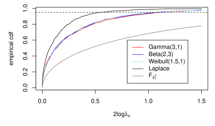
Figure 1: Monte Carlo distributions of $2\log\lambda_{n}$ for four distributions, $n=10^{4}$, $M=5\times 10^{3}$ replications, together with the exact distribution function of $\chi_{1}^{2}$.

Now for $\alpha\in(0,1)$ let $d_{\alpha}$ satisfy $P({\mathbb{D}}>d_{\alpha})=\alpha$. The following table gives

Table 2: Estimated critical values $d_{\alpha}$

$\alpha$	$.25$	$.20$	$.15$	$.10$	$.05$	$.01$
$d_{\alpha}$	$.40$	$.49$	$.61$	$.79$	$1.11$	$1.92$

a few estimated values for $d_{\alpha}$: These are based on $350,000$ Monte Carlo simulations each based on simulating $1\times 10^{6}$ observations from a standard normal. These values, and the simulated critical values for all $\alpha\in(0,1)$, are available in the logcondens.mode package [Doss, 2013a] in R [R Core Team, 2016].

Banerjee and Wellner [2001] study a likelihood ratio test in the context of constraints based on monotonicity, and find a universal limiting distribution, denote it ${\mathbb{D}}_{\text{mono}}$, for their likelihood ratio test. Comparison of the values in Table 2 with Table 2 of Banerjee and Wellner [2001] (particularly Method 2 in column 3 of that table) suggest, perhaps surprisingly, that $P(2{\mathbb{D}}\leq t)\approx P({\mathbb{D}}_{\text{mono}}\leq t)$ for $t\in{\mathbb{R}}$. It would be quite remarkable if this held exactly. We do not have any explanation for this observed phenomenon.

5.2 Comparisons via simulations

Code to compute the mode-constrained log-concave MLE, implement a corresponding test, and invert the family of tests to form confidence intervals is available in the logcondens.mode package [Doss, 2013a]. We can thus test our procedure and compare it to alternatives.

Romano [1988a] proposed and investigated two methods of forming confidence intervals for the mode of a unimodal density. His estimators of the mode and confidence intervals were based on the classical kernel density estimators of the density $f$ going back to Parzen [1962]. One method, which Romano called the “normal approximation method”, is based on the limiting normality of the kernel density estimator of the mode, together with a plug-in estimator of the asymptotic variance. Romano’s second method involved bootstrapping the mode estimator, and involved the choice of two bandwidths, one for the initial estimator to determine the mode, and a second (larger) bandwidth for the bootstrap sampling. The abstract of Romano [1988a] states: “In summary, the results are negative in the sense that a straightforward application of a naive bootstrap yields invalid inferences. In particular the bootstrap fails if resampling is done from the kernel density estimate.” That is, one must use a second (larger) bandwidth for the bootstrap resampling to achieve valid inference. This thus necessitates selection of two tuning parameters for the bootstrap procedure. Romano [1988a] notes in summarizing his simulation results:

… but the problem of constructing a confidence interval for the mode for smaller sample sizes remains a challenging one. In summary, the simulations reinforce the idea that generally automatic methods like the bootstrap need mathematical and numerical justification before their use can be recommended.

The bootstrap simulations that Romano [1988a] refers to in the previous quote are based on an underlying $N(0,1)$ or a $\chi_{4}^{2}$ distribution with a sample size of $n=100$. Romano [1988a] also performs simulations for the normal approximation method for the same underlying distributions and based on the same sample size. For the normal approximation method, a grid of bandwidths $h$ are used for the simulation. For the bootstrap, a matrix of bandwidth pairs $(h,b)$ (one for estimation, one for resampling) are used. Monte Carlo estimates of coverage probabilities are presented in Tables 1–4 of Romano [1988a].

In Figure 2 we consider the case of a true underlying $\chi_{4}^{2}$ distribution, and we plot all the estimated coverage probabilities of Romano’s bootstrap CI’s (blue; these are from Romano [1988a]’s Table 4) together with the target (ideal) coverage (green line) and the estimated coverage probabilities of our likelihood ratio (LR) based CI’s (magenta). As can be seen, the estimated coverage probabilities of our LR-based procedure are reasonably close to the target values without requiring any bandwidth choice.

Corresponding comparison plots based on Tables 1,2, and 3 of Romano [1988a], as well as tables of the simulated coverage probabilities, are given in Doss and Wellner [2016b]. We do not include them here due to space constraints. Doss and Wellner [2016b] also includes a Monte Carlo simulation study of lengths of the CI’s in some settings.

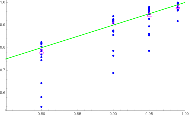
Figure 2: Coverage probabilities, Romano’s Table 4 compared with LR coverage probabilities, $\chi_{4}^{2}$ data, Bootstrap confidence intervals (blue dots); LR confidence intervals (magenta triangles). The green line is the nominal level.

Methods of bandwidth selection for various problems have received considerable attention in the period since Romano [1988a]; see especially Léger and Romano [1990], Mammen and Park [1997], Härdle, Marron and Wand [1990], Hall and Johnstone [1992], Ziegler [2001], Hazelton [1996a], Hazelton [1996b], and Samworth and Wand [2010]. Although bandwidth selection in connection with mode estimation is mentioned briefly by Léger and Romano [1990] (see their last paragraph, page 734), we are not aware of any specific proposal or detailed study of bandwidth selection methods in the problem of confidence intervals for the mode of a unimodal density. For this reason, we have not undertaken a full comparative study of possible methods here. Further comparisons of our LR based confidence intervals with methods based on kernel density estimates of the type studied by Romano [1988a] but incorporating current state of the art bandwidth selection procedures will be of interest.

5.3 Comparisons via data examples

We used our procedure for formation of modal confidence intervals (CI’s) on two real data sets, the rotational velocities of stars from the Bright Star Catalogue [Hoffleit and Warren, 1991] and daily log returns for the S&P $500$ stock market index. To see the former, see Section 5.3 of Doss and Wellner [2016b]. Here we discuss the $1006$ daily log returns for the S&P $500$ stock market index from January $1$, 2003 to December $29$, 2006. In Figure 3 we plot the data, a kernel density estimate with bandwidth $.13$ [Sheather and Jones, 1991], the log-concave MLE, and the $95$% confidence interval for the mode given by our likelihood ratio statistic. We also plot the maximum likelihood Gaussian density estimate, for comparison. The sample mean is $0.04$, the sample median is $0.081$, and the log-concave mode estimate is $0.17$. A $95$% CI’s for the mean is $[-0.004,0.09]$ and a $95$% CI for the median is $[.037,.122]$, [Hogg and Craig, 1970, pages 539–540]. Our likelihood ratio CI for the mode is $[0.10,0.21]$. Note that our confidence interval for the mode excludes $0$ and does not intersect with the CI for the mean. Thus, our procedure highlights some interesting features of the data and provides evidence for its non-normality. Also note that the lengths of the mean, median, and our LR-based mode CI are $0.094$, $0.085$, and $0.11$. Thus, despite the fact that our mode estimator does not generally have a $n^{-1/2}$ rate of convergence, the three confidence intervals are of fairly similar length on a dataset with $1006$ observations, which is encouraging for our mode CI procedure and for any future extensions (e.g., mode regression CI’s).

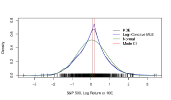
Figure 3: $1006$ S&P $500$ daily log returns for the years $2003$–$2006$

6 Further Problems and potential developments

6.1 Uniformity and rates of convergence

There is a long line of research giving negative results concerning nonparametric estimation, starting with Bahadur and Savage [1956], Blum and Rosenblatt [1966], Singh [1963, 1968], and continuing with Donoho [1988] and Pfanzagl [1998, 2000]. In particular, Pfanzagl [2000] considers a general setting involving estimators or confidence limits with optimal convergence rate $n^{-\rho}$ with $0<\rho<1/2$. He shows, under weak additional conditions, that: (i) there do not exist estimators which converge locally uniformly to a limit distribution; and (ii) there are no confidence limits with locally uniform asymptotic coverage probability. As an example he considers the mode of probability distributions $P$ on ${\mathbb{R}}$ with corresponding densities $p$ having a unique mode $M(p)$ and continuous second derivative in a neighborhood of $M(p)$. Pfanzagl [2000] also reproves the result of Has’minskii [1979] to the effect that the optimal rate of convergence of a mode estimator for such a class is $n^{-1/5}$. In this respect, we note that Balabdaoui, Rufibach and Wellner [2009] established a comparable lower bound for estimation of the mode in the class of log-concave densities with continuous second derivative at the mode; they obtained a constant which matches (up to absolute constants) the pointwise (fixed $P$) behavior of the plug-in log-concave MLE of the mode. Romano [1988b] gives a detailed treatment of minimax lower bounds for estimation of the mode under smoothness and curvature assumptions: assuming a bounded derivative of order $p$ in a neighborhood of the mode $M(f_{0})$, Romano shows in his Theorem 3.1 that the minimax rate for estimation of $M(f_{0})$ is $n^{-r}$ where $r=(p-1)/(2p+1)$. He also shows that when $p=3$, the rate $n^{-2/7}$ can be achieved by a kernel density estimator.

Our approach here has been to construct reasonable confidence intervals with pointwise (in $P$ or density $p$) correct asymptotic coverage without proof of any local uniformity properties. In view of the recent uniform rate results of Kim and Samworth [2016] we suspect that our new confidence intervals will (eventually) be shown to have some uniformity of convergence in their coverage probabilities over appropriate subclasses of the class of log-concave densities, but we leave the uniformity issues to future work.

6.2 Some further directions and open questions

But we now turn to discussion of some difficulties and potential for further work.

6.2.1 Relaxing the second derivative assumption:

As noted in the previous subsection, most of the available research concerning inference for $M(f)$ has assumed $f\in C^{2}(m,\mbox{loc})$ and $f^{(2)}(M(f))<0$. Second derivative type assumptions of this type are made in Parzen [1962], Has’minskii [1979], Eddy [1980], Donoho and Liu [1991], Romano [1988a, b], and Pfanzagl [2000]. Exceptions include Müller [1989], Ehm [1996], Herrmann and Ziegler [2004], Balabdaoui, Rufibach and Wellner [2009].

What happens if the second derivative curvature assumption does not hold, but instead is replaced by something either stronger or weaker, such as

$$f(m)-f(x)\leq C|x-m|^{r}$$

for some $C$ where $1\leq r<2$ (in the “stronger” case) or $2<r<\infty$ (in the “weaker” case)? It is natural to expect that it is easier to form confidence intervals for $m$ when $1\leq r<2$ holds, but that it is harder to form confidence intervals for $m$ when $2<r<\infty$. In fact, Balabdaoui, Rufibach and Wellner [2009] page 1313 gives the following result: if $f=\exp(\varphi)$ with $\varphi$ concave and where $\varphi^{(j)}(m)=0$ for $j=2,\ldots,k-1$ but $\varphi^{(k)}$ exists and is continuous in a neighborhood of $m$ with $\varphi^{(k)}(m)\not=0$, then

$$n^{1/(2k+1)}(\widehat{M}_{n}-m)\rightarrow_{d}C_{k}(f(m),\varphi^{(k)}(m))M(H_{k}^{(2)}).$$

Thus the convergence rate of the log-concave MLE of the mode is slower as $k$ increases. [On the other hand, by Theorem 2.1 of Balabdaoui, Rufibach and Wellner [2009], page 1305, the convergence rate of the MLE $\widehat{f}_{n}$ of $f$ at $m$ (and in a local neighborhood of $m$) is faster:

$$n^{k/(2k+1)}(\widehat{f}_{n}(m)-f(m))\rightarrow_{d}c_{k}(m,f)H_{k}^{(2)}(0).]$$

Furthermore the sketch of the proof of the limiting distribution of the likelihood ratio statistic in Section 4.1 (ignoring any remainder terms) together with the results of Balabdaoui, Rufibach and Wellner [2009], suggest that $2\log\lambda_{n}\rightarrow_{d}{\mathbb{D}}_{k}$ under $f\in{\cal P}_{m}\cap{\cal Z}_{k}$ where

$${\cal Z}_{k}=\{f\in{\cal P}:\ \varphi^{(j)}(m)=0,\ j=2,\ldots,k-1,\ \varphi^{(k)}(m)\not=0,\ \varphi\in C^{k}(m,\mbox{loc})\}$$

and where with $\varphi_{k}$ and $\varphi_{k}^{0}$ denoting the local limit processes in the white noise model (1.2) with drift term $g_{0}(t)=-12t^{2}$ replaced by $-(k+2)(k+1)|t|^{k}$,

$${\mathbb{D}}_{k}\equiv\int\{(\widehat{\phi}_{k}(v))^{2}-(\widehat{\phi}_{k}^{0}(v))^{2}\}dv.$$

We provide Monte Carlo evidence in support of this conjecture, by simulating $2\log\lambda_{n}$ based on some parent distributions with $k\neq 2$. The results are given in Figure 4. Figure 4 contains empirical distributions of $2\log\lambda_{n}$ (with $n=10^{4}$ and $M=5\times 10^{3}$) for $9$ parent distributions, as well as a plot of the df of a $\chi_{1}^{2}$ random variable; all of the curves from Figure 1 are present, including $F_{\chi_{1}^{2}}$, the Laplace (with $k=1$), the standard normal, Gamma$(3,1)$, Beta$(2,3)$, and Weibull$(1.5,1)$ (all four having $k=2$). We also add four parent distributions with $k>2$. We include parent densities proportional to $\exp\left\{-|x|^{j}/j\right\}$ for $x\in{\mathbb{R}}$, labelled “Subbotin$(j)$,” $j=3,4$ (having $k=j$). We also include parent densities proportional to $1-|x|^{j}$ for $x\in[-1,1]$, labelled “Bump$(j)$,” $j=3,4$ (with $k=j$). The (Monte Carlo estimators of) dfs based on the parent distributions with $k=3$ (estimating ${\mathbb{D}}_{3}$) are grouped together, and the dfs based on the parent distributions with $k=4$ (estimating ${\mathbb{D}}_{4}$) are similarly grouped together. Note that the (Monte Carlo estimator of) the distribution of ${\mathbb{D}}_{3}$ seems to be stochastically larger than the (Monte-Carlo estimator) of the distribution of ${\mathbb{D}}_{2}\equiv{\mathbb{D}}$, and that the distribution of ${\mathbb{D}}_{4}$ is apparently stochastically larger than that of ${\mathbb{D}}_{3}$.

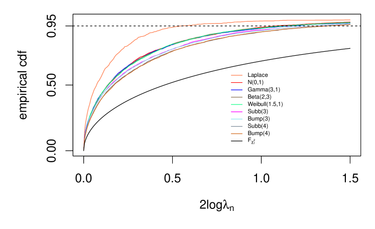
Figure 4: Empirical distributions of $2\log\lambda_{n}$ for $f\in{\cal P}_{m}\cap{\cal Z}_{k}$, $k\in\{2,3,4\}$ with $n=10^{4}$ and $M=5\times 10^{3}$ replications.

This raises several possibilities:

Option 1:

It seems likely that by choosing a critical value from the distribution of ${\mathbb{D}}_{6}$ (say), that the resulting confidence intervals will have correct coverage for $f\in{\cal P}\cap{\cal Z}_{6}$ with conservative coverage if we happen to have $f\in{\cal P}\cap{\cal Z}_{2}$ (in which case critical points from ${\mathbb{D}}={\mathbb{D}}_{2}$ would have sufficed), and anti-conservative coverage if the true $f$ belongs to ${\cal P}\cap({\cal Z}_{k}\setminus{\cal Z}_{6})$ for some $k\geq 8$.

Option 2:

Try to construct an adaptive procedure which first estimates $k$ (the degree of “flatness”) of the true $f\in{\cal P}$ (by $\hat{k}$ say), and then choose a critical point from the distribution of ${\mathbb{D}}_{\hat{k}}$.

We leave the investigation of both of these possibilities to future work.

6.2.2 Relaxing the assumption of log-concavity

It would also be of interest to relax the assumption of log-concavity used in the developments here. It would be very desirable to allow $f_{0}$ to be a completely arbitrary unimodal density, and allow the smoothness at the mode $M(f_{0})$ to vary as noted in the previous subsection. As a more realistic replacement for this ambitious goal, we might instead consider enlarging from the class of log-concave densities to some class of $s-$concave densities, ${\cal P}_{s}$ with $-1<s<0$; i.e. densities of the form $f_{0}=\phi_{0}^{1/s}$ with $\phi_{0}>0$ convex; see e.g. Koenker and Mizera [2010], Doss and Wellner [2016a], and Han and Wellner [2016]. Extensions in this direction will likely require further study of the Rényi divergence estimators studied in Han and Wellner [2016] and mode-constrained versions thereof. An interesting possible connection is that for the classes of $\alpha-$stable densities ${\cal S}_{\alpha}$ with $0<\alpha\leq 2$, we know that $f_{0}\in{\cal S}_{\alpha}$ is unimodal. Moreover, it is also known from Hall [1984] that for the symmetric $\alpha-$stable distributions $f_{0}^{\prime\prime}$ exists in a neighborhood of the mode $m=M(f_{0})$, and $f_{0}^{\prime\prime}(m)<0$. It is apparently not known if the $\alpha-$stable densities are $s-$concave for some $s\in(-1,0]$, even though this obviously holds in the (few) examples for which an explicit formula for the density $f_{0}\in{\cal S}_{\alpha}$ is available: for example for $f_{0}=$ Cauchy, $f_{0}\in{\cal S}_{1}\cap{\cal P}_{-1/2}$, while for Lévy’s completely asymmetric stable law, $f_{0}\in{\cal S}_{1/2}\cap{\cal P}_{-2/3}$, and of course, for $f_{0}=\$Gaussian, $f_{0}\in{\cal S}_{2}\cap{\cal P}_{0}$.

6.2.3 Mode inference in other contexts

The methods developed in this paper raise several questions about other settings in which inference about a convex function may be of interest.

1. Can we do inference for the maxima or minima in the contexts of estimation of intensity functions, of (bathtub-shaped) hazard functions [Jankowski and Wellner, 2009], or of regression functions? For instance, let $Y_{i}=r(x_{i})+\varepsilon_{i}$ where $\varepsilon_{i}$ are mean zero i.i.d. observations and $x_{i}$ are fixed numbers in ${\mathbb{R}}$. If we assume $r$ to be convex, then much is known about the least-squares estimator $\widehat{r}_{n}$ of $r$; see, e.g., Hildreth [1954], Hanson and Pledger [1976], Mammen [1991], and Groeneboom, Jongbloed and Wellner [2001a, b]. Can an argmin-constrained estimator $\widehat{r}_{n}^{0}$ be developed, in analogy with the estimator $\widehat{f}_{n}^{0}$, and used to develop likelihood ratio-based (or rather, residual sum-of-squares) tests and intervals for the location of the minimum of $r$? In such a problem, we conjecture that the universal component of the limit distribution of $\widehat{r}_{n}^{0}(m)$ will be the same as that studied in Theorem 1.1.

2. Can the techniques used here be applied to form tests and intervals for the value (or height) of a concave function, $f_{0}$, rather than argmax? Here, $f_{0}$ could be a log-concave density or a concave regression function (and other settings could be of interest). That is, can we develop an estimator $\widehat{f}_{n}^{0}$ based on the constraint that $f$ satisfies $f(x_{0})=y_{0}$ for $x_{0},y_{0}$ fixed, and use $\widehat{f}_{n}^{0}$ with an unconstrained estimator $\widehat{f}_{n}$ to form a likelihood ratio test for $f_{0}(x_{0})$? In the case where $f_{0}$ is a concave regression function, such a program has recently been studied by Doss [2018]. Can this be extended to the density case, where $f_{0}$ is log-concave?

3. Can inference for the mode be extended to semiparametric settings? For example can we form tests/intervals for the location of the minimum of an unknown convex “link” function $m_{0}$ in a single index model, $Y=m_{0}(\theta_{0}^{\prime}X)+\varepsilon$, where $X\in{\mathbb{R}}^{d}$, $Y\in{\mathbb{R}}$, $E(\varepsilon|X)=0$, and $m_{0}$ is assumed to be convex [Kuchibhotla, Patra and Sen, 2017; Chen and Samworth, 2016]? Can we form tests/intervals for a modal regression function, i.e. for $m_{0}$ where $Y=m_{0}(X)+\varepsilon$ where $\varepsilon$ has mode $0$?

6.2.4 Beyond dimension $d=1$:

It seems natural to consider generalizations of the present methods to the case of multivariate log-concave and $s-$concave densities. While there is a considerable amount of work on estimation of multivariate modes, mostly via kernel density estimation, much less seems to be available in terms of confidence sets or other inference tools. For some of this, see e.g. Tsybakov [1990], Abraham, Biau and Benoît [2003], Kim [1994], Klemelä [2005], Konakov [1973], Sager [1978], Samanta [1973]. On the other hand apparently very little is known about the multivariate mode estimator $M(\widehat{f}_{n})$ where $\widehat{f}_{n}$ is the log-concave density estimator for $f$ on ${\mathbb{R}}^{d}$ studied by Cule, Samworth and Stewart [2010] and Cule and Samworth [2010]. Further study of this estimator will very likely require considerable development of new methods for study of the pointwise and local properties of the log-concave density estimator $\widehat{f}_{n}$ when $d\geq 2$.

Appendix A Proofs

We now deal with the remainder terms defined in (4.9) in the course of our “proof sketch” for Theorem 1.1. We first deal with the “local” remainder terms $R_{n,j},\ R_{n,j}^{0}$ with $j\in\{2,3\}$ in Subsection A.1. The analysis of these local remainder terms depends crucially on Theorem 2.1. Subsection A.2 is dedicated to the proofs for the “non-local” remainder terms.

For a function $f\colon{\mathbb{R}}\to{\mathbb{R}}$, we let $\|f\|:=\sup_{x\in{\mathbb{R}}}|f(x)|$, and for a set $J\subset{\mathbb{R}}$ we let $\|f\|_{J}:=\sup_{x\in J}|f(x)|$.

A.1 The local remainder terms $R_{n,j},R_{n,j}^{0}$, $j\in\{2,3\}$

We first deal with the (easy) local remainder terms.

Proposition A.1.

Let $t_{n,1}=m-Mn^{-1/5}$ and $t_{n,2}=m+Mn^{-1/5}$ for $M>0$. Then the remainder terms $R_{n,2}$, $R_{n,2}^{0}$, $R_{n,3}$, and $R_{n,3}^{0}$ satisfy $nR_{n,j}=o_{p}(1)$ and $nR_{n,j}^{0}=o_{p}(1)$ for $j\in\{2,3\}$.

Proof.

Recall that the remainder terms $R_{n,2}$, $R_{n,2}^{0}$, $R_{n,3}$, and $R_{n,3}^{0}$ given by (4.4), (4.5), (4.7), and (4.8) are all of the form a constant times

$$\tilde{R}_{n}\equiv\int_{D_{n}}e^{\tilde{x}_{n}(u)}(\widehat{\varphi}_{n}(u)-\varphi_{0}(m))^{3}du,\ \ \ \mbox{or}$$

$$\tilde{R}_{n}^{0}\equiv\int_{D_{n}}e^{\tilde{x}_{n}^{0}(u)}(\widehat{\varphi}_{n}^{0}(u)-\varphi_{0}(m))^{3}du,$$

where $D_{n}$ is a (possibly random) interval of length $O_{p}(n^{-1/5})$ and $\tilde{x}_{n,j}$ converges in probability, uniformly in $u\in D_{n}$, to zero. But by Assumption 1 and by Theorem 2.1 Part A it follows that for any $M>0$ we have

$$\sup_{|t|\leq M}|\widehat{\varphi}_{n}(m+n^{-1/5}t)-\varphi_{0}(m)|$$

$$\leq \sup_{|t|\leq M}\left\{|\widehat{\varphi}_{n}(m+n^{-1/5}t)-\varphi_{0}(m+n^{-1/5}t)|+|\varphi_{0}(m+n^{-1/5}t)-\varphi_{0}(m)|\right\}$$

$$= O_{p}((n^{-1}\log n)^{2/5})+O(n^{-2/5})=O_{p}((n^{-1}\log n)^{2/5}),$$

and hence

$$n|\tilde{R}_{n}|=nO_{p}((n^{-1}\log n)^{6/5}\cdot n^{-1/5})=O_{p}(n^{-2/5}(\log n)^{6/5})=o_{p}(1),$$

By Assumption 1 and by Theorem 2.1 Part B it follows that for any $M>0$ we have

$$n|\tilde{R}_{n}^{0}|=nO_{p}((n^{-1}\log n)^{6/5}\cdot n^{-1/5})=O_{p}(n^{-2/5}(\log n)^{6/5})=o_{p}(1).$$

Note that the $o_{p}$ terms do not depend on $M$, by Theorem 2.1. This completes the proof of negligibility of the local error terms $R_{n,j},R_{n,j}^{0}$, $j\in\{2,3\}$. ∎

A.2 The global remainder terms $R_{n,1}$ and $R_{n,1}^{c}$

Recall that the remainder terms $R_{n,1}$ and $R_{n,1}^{c}$ are given by (4.2) and (4.3). Note that the integral in the definition of (4.3) is over $[X_{(1)},X_{(n)}]\setminus D_{n}$, and hence this term in particular has a global character. We will see later that $R_{n,1}$ also can be seen as having a global nature.

Outline: From now on, we will focus our analysis on the portion of $R_{n,1,t_{1},t_{2}}^{c}$ given by integrating over the left side, $[X_{(1)},t_{1}]$. Arguments for the integral over $[t_{2},X_{(n)}]$ are analogous. Thus, by a slight abuse of notation, define the one-sided counterpart to $R_{n,1,t_{1},t_{2}}^{c}$ from (4.3) for any $t<m$ by

$$\begin{split}R_{n,1,t}^{c}&\equiv\int_{[X_{(1)},t]}\widehat{\varphi}_{n}d\widehat{F}_{n}-\widehat{\varphi}_{n}^{0}d\widehat{F}_{n}^{0}-\int_{[X_{(1)},t]}(e^{\widehat{\varphi}_{n}}-e^{\widehat{\varphi}_{n}^{0}})\,d\lambda.\end{split}$$ (A.1)

Here $\lambda$ is Lebesgue measure (and is unrelated to the likelihood ratio $\lambda_{n}$). The analysis of $R_{n,1,t}^{c}$ is the greatest difficulty in understanding $2\log\lambda_{n}$. The proof that $R_{n,1,t_{n}}^{c}$ is $o_{p}(n^{-1})$ when $b\to\infty$ where $t_{n}=m-bn^{-1/5}$ is somewhat lengthy so we provide an outline here.

1. Step 1, Decomposition of $R_{n,1,t}^{c}$: Decompose $R_{n,1,t}^{c}$, to see that

   $$R_{n,1,t}^{c}=A_{n,t}^{1}+E_{n,t}^{1}-T_{n,t}^{1}=A_{n,t}^{2}+E_{n,t}^{2}+T_{n,t}^{2},$$ (A.2)

   where the summands $A_{n,t}^{i},E_{n,t}^{i},T_{n,t}^{i}$ are defined below (see (A.11) and the preceding text).

2. Step 2, Global $O_{p}(n^{-1})$ conclusion: In this section we use the fact that away from the mode, the characterizations of $\widehat{\varphi}_{n}$ and $\widehat{\varphi}_{n}^{0}$ are identical to study $T_{n}^{i}$, $i=1,2$, which are related to $\int_{[X_{(1)},t]}(\widehat{\varphi}_{n}-\widehat{\varphi}_{n}^{0})^{2}\widehat{f}_{n}d\lambda$. and $\int_{[X_{(1)},t]}(\widehat{\varphi}_{n}-\widehat{\varphi}_{n}^{0})^{2}\widehat{f}_{n}^{0}d\lambda$. We will show ${T}_{n}^{i}=O_{p}(n^{-1})$, $i=1,2$. Note $O_{p}(n^{-1})$ would be the size of the integral if it were over a local interval of length $O_{p}(n^{-1/5})$ (under our curvature assumptions), but here the integral is over an interval of constant length or larger, so this result is global in nature.

3. Step 3, Convert global $O_{p}$ to local $o_{p}$ to global $o_{p}$: Convert the global $O_{p}(n^{-1})$ conclusion over $T_{n}^{i}$ into an $o_{p}(n^{-1})$ conclusion over a interval of length $O_{p}(n^{-1/5})$ local to $m$. Feed this result back into the argument in Step 2, yielding $T_{n,t}^{i}=o_{p}(n^{-1}),$ $i=1,2$. Apply Lemma C.2 to show additionally that there exist knots of $\widehat{\varphi}_{n}$ and $\widehat{\varphi}_{n}^{0}$ that are $o_{p}(n^{-1/5})$ apart in an $O_{p}(n^{-1/5})$ length interval on which $\|\widehat{\varphi}_{n}^{0}-\widehat{\varphi}_{n}\|=o_{p}(n^{-2/5})$, $\|\widehat{f}_{n}^{0}-\widehat{f}_{n}\|=o_{p}(n^{-2/5})$, and $\|\widehat{F}_{n}^{0}-\widehat{F}_{n}\|=o_{p}(n^{-3/5})$.

4. Step 4, Concluding arguments: Return to the decomposition of $R_{n,1,t}^{c}$ given in Step 1; the terms given there depend on $\widehat{\varphi}_{n}^{0}-\widehat{\varphi}_{n}$, $\widehat{f}_{n}^{0}-\widehat{f}_{n}$, and $\widehat{F}_{n}^{0}-\widehat{F}_{n}$. Thus, using the results of Step 3 we can show $nR_{n,1,t}^{c}=o_{p}(1)$ as desired.

To finalize the argument, in Section A.3, we take $t_{n}=m-bn^{-1/5}$, but we also need to let $b\to\infty$. Thus, the $O_{p}$ and $o_{p}$ statements above need to hold uniformly in $b$.

A.2.1 Decomposition of $R_{n,1,t}^{c}$

We begin by decomposing $R_{n,1,t}^{c}$ for fixed $t<m$. By (C.2) with $\varphi_{1n}=\widehat{\varphi}_{n}$ and $\varphi_{2n}=\widehat{\varphi}_{n}^{0}$, we see that

$$R_{n,1,t}^{c} =\int_{[X_{(1)},t]}\left(\widehat{\varphi}_{n}\widehat{f}_{n}-\widehat{\varphi}_{n}^{0}\widehat{f}_{n}^{0}-\left(\widehat{\varphi}_{n}-\widehat{\varphi}_{n}^{0}+\frac{(\widehat{\varphi}_{n}-\widehat{\varphi}_{n}^{0})^{2}}{2}e^{\varepsilon_{n}^{1}}\right)\widehat{f}_{n}^{0}\right)\,d\lambda$$

$$=\int_{[X_{(1)},t]}\left(\widehat{\varphi}_{n}\widehat{f}_{n}-\widehat{\varphi}_{n}\widehat{f}_{n}^{0}-\frac{(\widehat{\varphi}_{n}-\widehat{\varphi}_{n}^{0})^{2}}{2}e^{\varepsilon_{n}^{1}}\widehat{f}_{n}^{0}\right)d\lambda$$

$$=\int_{[X_{(1)},t]}\left(\widehat{\varphi}_{n}(\widehat{f}_{n}-\widehat{f}_{n}^{0})-\frac{(\widehat{\varphi}_{n}-\widehat{\varphi}_{n}^{0})^{2}}{2}e^{\varepsilon_{n}^{1}}\widehat{f}_{n}^{0}\right)\,d\lambda,$$ (A.3)

where $\lambda$ is Lebesgue measure and $\varepsilon_{n}^{1}(x)$ lies between $0$ and $\widehat{\varphi}_{n}(x)-\widehat{\varphi}_{n}^{0}(x)$. Again applying (C.2) now with $\varphi_{1n}=\widehat{\varphi}_{n}^{0}$ and $\varphi_{2n}=\widehat{\varphi}_{n}$, we see that

$$R_{n,1,t}^{c} =\int_{[X_{(1)},t]}\left(\widehat{\varphi}_{n}\widehat{f}_{n}-\widehat{\varphi}_{n}^{0}\widehat{f}_{n}^{0}+\left(e^{\widehat{\varphi}_{n}^{0}-\widehat{\varphi}_{n}}-1\right)\widehat{f}_{n}\right)\,d\lambda$$

$$=\int_{[X_{(1)},t]}\left(\widehat{\varphi}_{n}\widehat{f}_{n}-\widehat{\varphi}_{n}^{0}\widehat{f}_{n}^{0}+\left(\widehat{\varphi}_{n}^{0}-\widehat{\varphi}_{n}+\frac{(\widehat{\varphi}_{n}^{0}-\widehat{\varphi}_{n})^{2}}{2}e^{\varepsilon_{n}^{2}}\right)\widehat{f}_{n}\right)\,d\lambda$$

$$=\int_{[X_{(1)},t]}\left(\widehat{\varphi}_{n}^{0}(\widehat{f}_{n}-\widehat{f}_{n}^{0})+\frac{(\widehat{\varphi}_{n}^{0}-\widehat{\varphi}_{n})^{2}}{2}e^{\varepsilon_{n}^{2}}\widehat{f}_{n}\right)\,d\lambda,$$ (A.4)

where $\varepsilon_{n}^{2}$ lies between $0$ and $\widehat{\varphi}_{n}^{0}(x)-\widehat{\varphi}_{n}(x)$. For a function $f(x)$, recall the notation $f_{s}(x)=f(x)-f(s)$ for $x\leq s$ and $f_{s}(x)=0$ for $x\geq s$. Now define $A^{i}_{n,t}\equiv A^{i}_{n}$, $i=1,2$ by

$$A_{n}^{1}\equiv\int_{[X_{(1)},t]}\widehat{\varphi}_{n,t}\,d\left(\mathbb{F}_{n}-\widehat{F}_{n}^{0}\right)\quad\mbox{ and }\quad A_{n}^{2}\equiv\int_{[X_{(1)},t]}\widehat{\varphi}_{n,t}^{0}d\left(\widehat{F}_{n}-\mathbb{F}_{n}\right)$$ (A.5)

and define $E_{n,t}^{1}\equiv E_{n}^{1}$ to be

$$\begin{split}&\int_{(\tau,t]}\widehat{\varphi}_{n,t}\,d\left(\widehat{F}_{n}-\mathbb{F}_{n}\right)+\widehat{\varphi}_{n}(t)(\widehat{F}_{n}(t)-\widehat{F}_{n}^{0}(t))\\ &+(\widehat{\varphi}_{n}(\tau)-\widehat{\varphi}_{n}(t))(\widehat{F}_{n}(\tau)-\mathbb{F}_{n}(\tau))\end{split}$$ (A.6)

and $E_{n,t}^{2}\equiv E_{n}^{2}$ to be

$$\begin{split}&\int_{(\tau^{0},t]}\widehat{\varphi}_{n,t}^{0}d\left(\mathbb{F}_{n}-\widehat{F}_{n}^{0}\right)+\widehat{\varphi}_{n}^{0}(t)(\widehat{F}_{n}(t)-\widehat{F}_{n}^{0}(t))\\ &+(\widehat{\varphi}_{n}^{0}(\tau^{0})-\widehat{\varphi}_{n}^{0}(t))(\mathbb{F}_{n}(\tau^{0})-\widehat{F}_{n}^{0}(\tau^{0})),\end{split}$$ (A.7)

where $\tau\equiv\tau_{-}(t)=\sup S(\widehat{\varphi}_{n})\cap(-\infty,t]$ and $\tau^{0}\equiv\tau_{-}^{0}(t)=\sup S(\widehat{\varphi}_{n}^{0})\cap(-\infty,t]$. We will assume that

$$\tau\leq\tau^{0}$$

without loss of generality, because the arguments are symmetric in $\widehat{\varphi}_{n}$ and $\widehat{\varphi}_{n}^{0}$, since we will be arguing entirely on one side of the mode.

Our next lemma will decompose the first terms in (A.3) and (A.4), into $A_{n}^{i}+E_{n}^{i}$, $i=1,2$. The crucial observation is that $A_{n}^{1}\leq 0$ and $A_{n}^{2}\geq 0$, by taking $\Delta=\widehat{\varphi}_{n,t}$ and $\Delta=\widehat{\varphi}_{n,t}^{0}$ in the characterization theorems for the constrained and unconstrained MLEs, Theorem 2.2 A and B of Doss and Wellner [2018]. Note that since $t\leq m$, $\widehat{\varphi}_{n,t}$ has modal interval containing $m$.

Lemma A.2.

Let all terms be as defined above. We then have

$$\begin{split}\int_{[X_{(1)},t]}\widehat{\varphi}_{n}(\widehat{f}_{n}-\widehat{f}_{n}^{0})d\lambda&=A_{n,t}^{1}+E_{n,t}^{1}\end{split}$$ (A.8)

and

$$\begin{split}\int_{[X_{(1)},t]}\widehat{\varphi}_{n}^{0}(\widehat{f}_{n}-\widehat{f}_{n}^{0})d\lambda&=A_{n,t}^{2}+E_{n,t}^{2}.\end{split}$$ (A.9)

Proof.

We first show (A.8). We can see $\int_{[X_{(1)},t]}\widehat{\varphi}_{n}(\widehat{f}_{n}-\widehat{f}_{n}^{0})$ equals

$$\int_{[X_{(1)},t]}(\widehat{\varphi}_{n,\tau_{-}}+\widehat{\varphi}_{n}-\widehat{\varphi}_{n,\tau_{-}})\widehat{f}_{n}d\lambda-\int_{[X_{(1)},t]}(\widehat{\varphi}_{n,t}+\widehat{\varphi}_{n}-\widehat{\varphi}_{n,t})\widehat{f}_{n}^{0}d\lambda,$$

and since $\int\widehat{\varphi}_{n,\tau_{-}}\,d\left(\mathbb{F}_{n}-\widehat{F}_{n}\right)=0$, this equals

$$\int_{[X_{(1)},\tau_{-}]}\widehat{\varphi}_{n,\tau_{-}}d\mathbb{F}_{n}+\int_{[X_{(1)},\tau_{-}]}(\widehat{\varphi}_{n}-\widehat{\varphi}_{n,\tau_{-}})\widehat{f}_{n}d\lambda+\int_{(\tau_{-},t]}\widehat{\varphi}_{n}\widehat{f}_{n}d\lambda$$

$$\quad-\left(\int_{[X_{(1)},t]}\widehat{\varphi}_{n,t}\widehat{f}_{n}^{0}d\lambda+\widehat{\varphi}_{n}(t)\widehat{F}_{n}^{0}(t)\right)$$

$$=\int_{[X_{(1)},t]}\widehat{\varphi}_{n,t}d\mathbb{F}_{n}+\int_{[X_{(1)},\tau_{-}]}(\widehat{\varphi}_{n,\tau_{-}}-\widehat{\varphi}_{n,t})d\mathbb{F}_{n}-\int_{(\tau_{-},t]}\widehat{\varphi}_{n,t}d\mathbb{F}_{n}$$

$$\quad+\int_{[X_{(1)},\tau_{-}]}\widehat{\varphi}_{n}(\tau_{-})\widehat{f}_{n}d\lambda+\int_{(\tau_{-},t]}\widehat{\varphi}_{n}\widehat{f}_{n}d\lambda-\left(\int\widehat{\varphi}_{n,t}\widehat{f}_{n}^{0}d\lambda+\widehat{\varphi}_{n}(t)\widehat{F}_{n}^{0}(t)\right)$$

$$=\int_{[X_{(1)},t]}\widehat{\varphi}_{n,t}\,d\left(\mathbb{F}_{n}-\widehat{F}_{n}^{0}\right)+\left(\widehat{\varphi}_{n}(t)-\widehat{\varphi}_{n}(\tau_{-})\right)\mathbb{F}_{n}(\tau_{-})-\int_{(\tau_{-},t]}\widehat{\varphi}_{n}d\mathbb{F}_{n}$$

$$\quad+\widehat{\varphi}_{n}(t)(\mathbb{F}_{n}(t)-\mathbb{F}_{n}(\tau_{-}))+\widehat{\varphi}_{n}(\tau_{-})\widehat{F}_{n}(\tau_{-})+\int_{(\tau_{-},t]}\widehat{\varphi}_{n}\widehat{f}_{n}d\lambda-\widehat{\varphi}_{n}(t)\widehat{F}_{n}^{0}(t),$$

which equals

$$\begin{split}&\int\widehat{\varphi}_{n,t}d\left(\mathbb{F}_{n}-\widehat{F}_{n}^{0}\right)+\int_{(\tau_{-},t]}\widehat{\varphi}_{n}d\left(\widehat{F}_{n}-\mathbb{F}_{n}\right)\\ &+\widehat{\varphi}_{n}(t)(\mathbb{F}_{n}(t)-\widehat{F}_{n}^{0}(t))+\widehat{\varphi}_{n}(\tau_{-})(\widehat{F}_{n}(\tau_{-})-\mathbb{F}_{n}(\tau_{-}))\end{split}$$

which equals

$$\begin{split}&\int\widehat{\varphi}_{n,t}d\left(\mathbb{F}_{n}-\widehat{F}_{n}^{0}\right)+\int_{(\tau_{-},t]}\widehat{\varphi}_{n,t}d\left(\widehat{F}_{n}-\mathbb{F}_{n}\right)\\ &+\widehat{\varphi}_{n}(t)(\widehat{F}_{n}(t)-\widehat{F}_{n}^{0}(t))+(\widehat{\varphi}_{n}(\tau_{-})-\widehat{\varphi}_{n}(t))(\widehat{F}_{n}(\tau_{-})-\mathbb{F}_{n}(\tau_{-})),\end{split}$$

as desired.

Now we show (A.9). We see $\int_{[X_{(1)},t]}\widehat{\varphi}_{n}^{0}(\widehat{f}_{n}-\widehat{f}_{n}^{0})d\lambda$ equals

$$\int_{[X_{(1)},t]}\left(\widehat{\varphi}_{n,t}^{0}+\widehat{\varphi}_{n}^{0}-\widehat{\varphi}_{n,t}\right)\widehat{f}_{n}d\lambda-\int_{[X_{(1)},t]}\left(\widehat{\varphi}_{n,\tau^{0}_{-}}^{0}+\widehat{\varphi}_{n}^{0}-\widehat{\varphi}_{n,\tau^{0}_{-}}^{0}\right)\widehat{f}_{n}^{0}d\lambda$$

and since $\int\widehat{\varphi}_{n,\tau^{0}_{-}}^{0}d(\mathbb{F}_{n}-\widehat{F}_{n}^{0})=0$, this equals

$$\int_{[X_{(1)},t]}\widehat{\varphi}_{n,t}^{0}\widehat{f}_{n}d\lambda+\widehat{\varphi}_{n}^{0}(t)\widehat{F}_{n}(t)-\bigg{[}\int\widehat{\varphi}_{n,\tau^{0}_{-}}^{0}d\mathbb{F}_{n}+\int_{[X_{(1)},\tau^{0}_{-}]}\widehat{\varphi}_{n}^{0}(\tau^{0}_{-})\widehat{f}_{n}^{0}d\lambda$$

$$\hskip 130.0002pt+\int_{(\tau^{0}_{-},t]}\widehat{\varphi}_{n}^{0}\widehat{f}_{n}^{0}d\lambda\bigg{]},$$

which equals

$$\int_{[X_{(1)},t]}\widehat{\varphi}_{n,t}^{0}\widehat{f}_{n}d\lambda+\widehat{\varphi}_{n}^{0}(t)\widehat{F}_{n}(t)-\bigg{[}\int_{[X_{(1)},t]}\widehat{\varphi}_{n,t}^{0}d\mathbb{F}_{n}$$

$$+\int_{[X_{(1)},t]}(\widehat{\varphi}_{n,\tau^{0}_{-}}^{0}-\widehat{\varphi}_{n,t}^{0})d\mathbb{F}_{n}+\widehat{\varphi}_{n}^{0}(\tau^{0}_{-})\widehat{F}_{n}^{0}(\tau^{0}_{-})+\int_{(\tau^{0}_{-},t]}\widehat{\varphi}_{n}^{0}\widehat{f}_{n}^{0}d\lambda\bigg{]}$$

which equals

$$\int_{[X_{(1)},t]}\widehat{\varphi}_{n,t}^{0}d(\widehat{F}_{n}-\mathbb{F}_{n})+\widehat{\varphi}_{n}^{0}(t)\widehat{F}_{n}(t)-\bigg{[}\int_{[X_{(1)},\tau^{0}_{-}]}(\widehat{\varphi}_{n}^{0}(t)-\widehat{\varphi}_{n}^{0}(\tau^{0}_{-}))d\mathbb{F}_{n}$$

$$\quad-\int_{(\tau^{0},t]}\widehat{\varphi}_{n}^{0}d\mathbb{F}_{n}+\int_{(\tau^{0}_{-},t]}\widehat{\varphi}_{n}^{0}(t)d\mathbb{F}_{n}+\widehat{\varphi}_{n}^{0}(\tau^{0}_{-})\widehat{F}_{n}^{0}(\tau^{0}_{-})+\int_{(\tau^{0}_{-},t]}\widehat{\varphi}_{n}^{0}\widehat{f}_{n}^{0}d\lambda\bigg{]}$$

which equals

$$\int_{[X_{(1)},t]}\widehat{\varphi}_{n,t}^{0}d(\widehat{F}_{n}-\mathbb{F}_{n})+\int_{(\tau^{0}_{-},t]}\widehat{\varphi}_{n}^{0}d(\mathbb{F}_{n}-\widehat{F}_{n}^{0})+\widehat{\varphi}_{n}^{0}(t)\widehat{F}_{n}(t)+\widehat{\varphi}_{n}^{0}(\tau^{0}_{-})\mathbb{F}_{n}(\tau^{0}_{-})$$

$$\quad-\widehat{\varphi}_{n}^{0}(t)\mathbb{F}_{n}(\tau^{0}_{-})-\widehat{\varphi}_{n}^{0}(t)(\mathbb{F}_{n}(t)-\mathbb{F}_{n}(\tau^{0}_{-}))-\widehat{\varphi}_{n}^{0}(\tau^{0}_{-})\widehat{F}_{n}^{0}(\tau^{0}_{-})$$

which equals

$$\int_{[X_{(1)},t]}\widehat{\varphi}_{n,t}^{0}d(\widehat{F}_{n}-\mathbb{F}_{n})+\int_{(\tau^{0}_{-},t]}\widehat{\varphi}_{n}^{0}d(\mathbb{F}_{n}-\widehat{F}_{n}^{0})$$

$$+\widehat{\varphi}_{n}^{0}(t)(\widehat{F}_{n}(t)-\mathbb{F}_{n}(t))+\widehat{\varphi}_{n}^{0}(\tau^{0}_{-})(\mathbb{F}_{n}(\tau^{0}_{-})-\widehat{F}_{n}^{0}(\tau^{0}_{-}))$$

which equals

$$\int_{[X_{(1)},t]}\widehat{\varphi}_{n,t}^{0}d\left(\widehat{F}_{n}-\mathbb{F}_{n}\right)+\int_{(\tau^{0}_{-},t]}\widehat{\varphi}_{n,t}^{0}d\left(\mathbb{F}_{n}-\widehat{F}_{n}^{0}\right)+\widehat{\varphi}_{n}^{0}(t)(\widehat{F}_{n}(t)-\widehat{F}_{n}^{0}(t))$$

$$\quad+(\widehat{\varphi}_{n}^{0}(\tau^{0}_{-})-\widehat{\varphi}_{n}^{0}(t))(\mathbb{F}_{n}(\tau^{0}_{-})-\widehat{F}_{n}^{0}(\tau^{0}_{-})),$$

as desired. ∎

Define $T_{n,t}^{i}\equiv T_{n}^{i}$, $i=1,2$, by

$$T_{n}^{1}=\int_{[X_{(1)},t]}\frac{(\widehat{\varphi}_{n}-\widehat{\varphi}_{n}^{0})^{2}}{2}e^{\varepsilon_{n}^{1}}\widehat{f}_{n}^{0}d\lambda\quad\mbox{ and }\quad T_{n}^{2}=\int_{[X_{(1)},t]}\frac{(\widehat{\varphi}_{n}-\widehat{\varphi}_{n}^{0})^{2}}{2}e^{\varepsilon_{n}^{2}}\widehat{f}_{n}d\lambda,$$ (A.10)

so that

$$R_{n,1,t}^{c}=A_{n,t}^{1}+E_{n,t}^{1}-T_{n,t}^{1}=A_{n,t}^{2}+E_{n,t}^{2}+T_{n,t}^{2}.$$ (A.11)

by (A.3) and (A.4). Recall (from page A.2.1) that $A_{n}^{1}\leq 0\leq A_{n}^{2}$. Thus

$$E_{n}^{1}-E_{n}^{2}\geq E_{n}^{1}-E_{n}^{2}-T_{n}^{2}-T_{n}^{1}=A_{n}^{2}-A_{n}^{1}\geq\begin{cases}&A_{n}^{2}\geq 0,\\ &-A_{n}^{1}\geq 0.\end{cases}$$ (A.12)

To see that $R_{n,1}^{c}=O_{p}(n^{-1})$ we need to see that $E_{n}^{i},A_{n}^{i},$ and $T_{n}^{i}$ are each $O_{p}(n^{-1})$ (for, say, $i=1$). We can see already that $E_{n}^{1}-E_{n}^{2}=O_{p}(n^{-1})$ (by direct analysis of the terms in $E_{n}^{1}-E_{n}^{2}$ from (A.6) and (A.7)), which yields that $A_{n}^{1}$ and $A_{n}^{2}$ are both $O_{p}(n^{-1})$. However, it is clear that we also need to analyze $T_{n}^{1}+T_{n}^{2}$ to understand $R_{n,1}^{c}$. We need to show that $T_{n,t}^{1}+T_{n,t}^{2}$ is $O_{p}(n^{-1})$ to see that $R_{n,1,t}^{c}=O_{p}(n^{-1})$; but we will also be able to use that $T_{n,t}^{1}+T_{n,t}^{2}=O_{p}(n^{-1})$ to then find $t^{*}$ values such that $T_{n,t^{*}}^{1}+T_{n,t^{*}}^{2}=o_{p}(n^{-1})$, which will allow us to argue in fact that $E_{n,t^{*}}^{1}+E_{n,t^{*}}^{2}=o_{p}(n^{-1})$ (rather than just $O_{p}(n^{-1})$), and thus that $R_{n,1,t^{*}}^{c}=o_{p}(n^{-1})$, as is eventually needed. Thus, we will now turn our attention to studying $T_{n}^{1}+T_{n}^{2}$. Afterwards, we will study

$$R_{n,1,t}^{c}=(A_{n,t}^{1}+E_{n,t}^{1}-T_{n,t}^{1}+A_{n,t}^{2}+E_{n,t}^{2}+T_{n,t}^{2})/2,$$ (A.13)

from (A.11). From seeing $T_{n,t^{*}}^{1}+T_{n,t^{*}}^{2}=o_{p}(n^{-1})$, we will be able to conclude that $A_{n,t^{*}}^{1}+A_{n,t^{*}}^{2}$ and $E_{n,t^{*}}^{1}+E_{n,t^{*}}^{2}$ are also $o_{p}(n^{-1})$, as desired. Then we can conclude $R_{n,1,t^{*}}^{c}=o_{p}(n^{-1})$.

A.2.2 Show ${T}_{n}^{i}=O_{p}(n^{-1})$, $i=1,2$

The next lemma shows that terms that are nearly identical to $T_{n}^{i}$ are $O_{p}(n^{-1})$. The difference between the integrand in the terms in the lemma and the integrand defining $T_{n}^{i}$ is that $\varepsilon_{n}^{i}$ is replaced by a slightly different $\tilde{\varepsilon}_{n}^{i}$. Previously, we considered $t$ to be fixed, whereas now we will have it vary with $n$.

Lemma A.3.

Let $t_{n}<m$ be a (potentially random) sequence such that

$$t_{n}\leq\max\left(S(\widehat{\varphi}_{n})\cup S(\widehat{\varphi}_{n}^{0})\right)\cap(-\infty,m).$$ (A.14)

Let

$$\tilde{T}_{n,t}^{1}=\int_{[X_{(1)},t_{n}]}\left(\widehat{\varphi}_{n}^{0}-\widehat{\varphi}_{n}\right)^{2}e^{\tilde{\varepsilon}_{n}^{1}}\widehat{f}_{n}^{0}d\lambda\;\mbox{ and }\;\tilde{T}_{n,t}^{2}=\int_{[X_{(1)},t_{n}]}\left(\widehat{\varphi}_{n}^{0}-\widehat{\varphi}_{n}\right)^{2}e^{\tilde{\varepsilon}_{n}^{2}}\widehat{f}_{n}d\lambda,$$ (A.15)

where $\tilde{\varepsilon}_{n}^{1}(x)$ lies between $\widehat{\varphi}_{n}(x)-\widehat{\varphi}_{n}^{0}(x)$ and $0$, and $\tilde{\varepsilon}_{n}^{2}(x)$ lies between $\widehat{\varphi}_{n}^{0}(x)-\widehat{\varphi}_{n}(x)$ and $0$, and are defined in (A.23) in the proof. Then we have

$$\tilde{T}_{n,t_{n}}^{i}=O_{p}(n^{-1})\quad\text{ for }i=1,2.$$ (A.16)

Proof.

For a function $f(x)$, recall the notation $f_{s}(x)=f(x)-f(s)$ for $x\leq s$ and $f_{s}(x)=0$ for $x\geq s$. Let $\tau\in S(\widehat{\varphi}_{n})$ and $\tau^{0}\in S(\widehat{\varphi}_{n}^{0})$, and assume that

$$\tau\leq\tau^{0}<m.$$ (A.17)

(The argument is symmetric in $\widehat{\varphi}_{n}$ and $\widehat{\varphi}_{n}^{0}$, so we may assume this without loss of generality.) We will show the lemma holds for the case $t_{n}=\tau^{0}$, and then the general $t_{n}\leq\tau^{0}$ case follows since the integral is increasing in $t_{n}$. Now, because $\widehat{\varphi}_{n,\tau}^{0}$ is concave, for $\varepsilon\leq 1$, the function $\widehat{\varphi}_{n}(x)+\varepsilon(\widehat{\varphi}_{n,\tau}^{0}(x)-\widehat{\varphi}_{n,\tau}(x))$ is concave. So, by Theorem 2.2, page 43, of Dümbgen and Rufibach [2009], we have

$$\int(\widehat{\varphi}_{n,\tau}^{0}-\widehat{\varphi}_{n,\tau})d(\mathbb{F}_{n}-\widehat{F}_{n})\leq 0.$$ (A.18)

Similarly, if $\tau^{0}$ is a knot of $\widehat{\varphi}_{n}^{0}$ and is less than the mode, then since $\widehat{\varphi}_{n}^{0}(x)+\varepsilon\left(\widehat{\varphi}_{n,\tau^{0}}(x)-\widehat{\varphi}_{n,\tau^{0}}^{0}(x)\right)$ is concave with mode at $m$ for $\varepsilon$ small (since $\widehat{\varphi}_{n,\tau^{0}}(x)-\widehat{\varphi}_{n,\tau^{0}}^{0}(x)$ is only nonzero on the left side of the mode), by the characterization Theorem 2.2 B of Doss and Wellner [2018], we have

$$\int(\widehat{\varphi}_{n,\tau^{0}}-\widehat{\varphi}_{n,\tau^{0}}^{0})d(\mathbb{F}_{n}-\widehat{F}_{n}^{0})\leq 0.$$

Then setting $II_{n,\tau^{0}}^{L}:=\int_{[X_{(1)},\tau^{0}]}\left(\widehat{\varphi}_{n}-\widehat{\varphi}_{n}^{0}\right)d\left(\mathbb{F}_{n}-\widehat{F}_{n}^{0}\right)$, we have

$$0 \geq\int_{[X_{(1)},\tau^{0}]}\left(\widehat{\varphi}_{n,\tau^{0}}-\widehat{\varphi}_{n,\tau^{0}}^{0}\right)d\left(\mathbb{F}_{n}-\widehat{F}_{n}^{0}\right)$$ (A.19)

$$=II_{n,\tau^{0}}^{L}-\left(\widehat{\varphi}_{n}(\tau^{0})-\widehat{\varphi}_{n}^{0}(\tau^{0})\right)\left(\mathbb{F}_{n}(\tau^{0})-\widehat{F}_{n}^{0}(\tau^{0})\right).$$ (A.20)

And setting $I_{n,\tau^{0}}^{L}:=\int_{[X_{(1)},\tau^{0}]}\left(\widehat{\varphi}_{n}^{0}-\widehat{\varphi}_{n}\right)d\left(\mathbb{F}_{n}-\widehat{F}_{n}\right)$, we have

$$\begin{split}I_{n,\tau^{0}}^{L}&=\int_{[X_{(1)},\tau]}\left(\widehat{\varphi}_{n}^{0}(u)-\widehat{\varphi}_{n}^{0}(\tau)\right)d\left(\mathbb{F}_{n}-\widehat{F}_{n}\right)(u)\\ &\quad-\int_{[X_{(1)},\tau]}\left(\widehat{\varphi}_{n}(u)-\widehat{\varphi}_{n}(\tau)\right)d\left(\mathbb{F}_{n}-\widehat{F}_{n}\right)(u)\\ &\quad+\left(\widehat{\varphi}_{n}^{0}(\tau)-\widehat{\varphi}_{n}(\tau)\right)\int_{[X_{(1)},\tau]}d\left(\mathbb{F}_{n}-\widehat{F}_{n}\right)\\ &\quad+\int_{(\tau,\tau^{0}]}\left(\widehat{\varphi}_{n}^{0}-\widehat{\varphi}_{n}\right)d\left(\mathbb{F}_{n}-\widehat{F}_{n}\right),\end{split}$$ (A.21)

and, since the first two summands together yield the left hand side of (A.18), we have

$$I_{n,\tau^{0}}^{L}\leq\left(\widehat{\varphi}_{n}^{0}(\tau)-\widehat{\varphi}_{n}(\tau)\right)\int_{[X_{(1)},\tau]}d\left(\mathbb{F}_{n}-\widehat{F}_{n}\right)+\int_{(\tau,\tau^{0}]}\left(\widehat{\varphi}_{n}^{0}-\widehat{\varphi}_{n}\right)d\left(\mathbb{F}_{n}-\widehat{F}_{n}\right).$$ (A.22)

Now, we apply (C.1) of Lemma C.1 to see that

$$I_{n,\tau^{0}}^{L}+II_{n,\tau^{0}}^{L} =\int_{[X_{(1)},\tau^{0}]}\left(\widehat{\varphi}_{n}^{0}-\widehat{\varphi}_{n}\right)d\left(\widehat{F}_{n}^{0}-\widehat{F}_{n}\right)$$

$$=\begin{cases}&\int_{X_{(1)}}^{\tau^{0}}\left(\widehat{\varphi}_{n}^{0}-\widehat{\varphi}_{n}\right)^{2}e^{\tilde{\varepsilon}_{n}^{1}}\widehat{f}_{n}^{0}d\lambda\geq 0,\\ &\int_{X_{(1)}}^{\tau^{0}}\left(\widehat{\varphi}_{n}^{0}-\widehat{\varphi}_{n}\right)^{2}e^{\tilde{\varepsilon}_{n}^{2}}\widehat{f}_{n}d\lambda\geq 0,\end{cases}$$ (A.23)

where $\tilde{\varepsilon}_{n}^{2}(x)$ lies between $\widehat{\varphi}_{n}^{0}(x)-\widehat{\varphi}_{n}(x)$ and $0$ and $\tilde{\varepsilon}_{n}^{1}(x)$ lies between $\widehat{\varphi}_{n}(x)-\widehat{\varphi}_{n}^{0}(x)$ and $0$. By (A.20) and (A.22), (A.23) is bounded above by

$$\begin{split}&\left(\widehat{\varphi}_{n}^{0}(\tau)-\widehat{\varphi}_{n}(\tau)\right)\int_{[X_{(1)},\tau]}d\left(\mathbb{F}_{n}-\widehat{F}_{n}\right)+\int_{(\tau,\tau^{0}]}\left(\widehat{\varphi}_{n}^{0}-\widehat{\varphi}_{n}\right)d\left(\mathbb{F}_{n}-\widehat{F}_{n}\right)\\ &\quad+\left(\widehat{\varphi}_{n}(\tau^{0})-\widehat{\varphi}_{n}^{0}(\tau^{0})\right)\left(\mathbb{F}_{n}(\tau^{0})-\widehat{F}_{n}^{0}(\tau^{0})\right).\end{split}$$ (A.24)

By Proposition 7.1 of Doss and Wellner [2018] and Lemma 4.5 of Balabdaoui, Rufibach and Wellner [2009], $\sup_{t\in[\tau,\tau^{0}]}\left|\widehat{\varphi}_{n}^{0}(t)-\widehat{\varphi}_{n}(t)\right|=O_{p}(n^{-2/5})$. By Corollary 2.5 of Dümbgen and Rufibach [2009],

$$\left|\int_{[X_{(1)},\tau]}d\left(\mathbb{F}_{n}-\widehat{F}_{n}\right)\right|\leq 1/n,$$

so the first term in the above display is $O_{p}(n^{-7/5})$. Similarly, by Corollary 2.7B of Doss and Wellner [2018], $\left|\mathbb{F}_{n}(\tau^{0})-\widehat{F}_{n}^{0}(\tau^{0})\right|\leq 1/n$, so the last term in the previous display is $O_{p}(n^{-7/5})$. We can also see that the middle term in the previous display equals

$$\begin{split}&(\widehat{\varphi}_{n}^{0}-\widehat{\varphi}_{n})(\tau^{0})(\mathbb{F}_{n}-\widehat{F}_{n})(\tau^{0})-(\widehat{\varphi}_{n}^{0}-\widehat{\varphi}_{n})(\tau)(\mathbb{F}_{n}-\widehat{F}_{n})(\tau)\\ &\ \ -\ \int_{(\tau,\tau^{0}]}(\mathbb{F}_{n}-\widehat{F}_{n})(\widehat{\varphi}_{n}^{0}-\widehat{\varphi}_{n})^{\prime}d\lambda.\end{split}$$ (A.25)

Now the middle term in the previous display is $O_{p}(n^{-7/5})$. For the last two terms, we apply Lemma C.4 taking $I=[\tau,\tau^{0}]$ to see that

$$\sup_{t\in(\tau,\tau^{0}]}n^{3/5}\left|\int_{(\tau,t]}d\left(\mathbb{F}_{n}-\widehat{F}_{n}\right)\right|=O_{p}(1).$$

Thus, using Proposition 7.1 of Doss and Wellner [2018] and Lemma 4.5 of Balabdaoui, Rufibach and Wellner [2009], we have

$$\int_{(\tau,\tau^{0}]}(\mathbb{F}_{n}-\widehat{F}_{n})(\widehat{\varphi}_{n}^{0}-\widehat{\varphi}_{n})^{\prime}d\lambda=O_{p}(n^{-4/5})\int_{(\tau,\tau^{0}]}d\lambda=O_{p}(n^{-1}),$$ (A.26)

so we have now shown that (A.25) is $O_{p}(n^{-1})$, so the middle term in (A.24) is $O_{p}(n^{-1})$. Thus, (A.24) is $O_{p}(n^{-1})$, and since (A.24) bounds (A.23) we can conclude that

$$\int_{X_{(1)}}^{\tau^{0}}\left(\widehat{\varphi}_{n}^{0}-\widehat{\varphi}_{n}\right)^{2}e^{\tilde{\varepsilon}_{n}^{1}}\widehat{f}_{n}^{0}d\lambda=\int_{X_{(1)}}^{\tau^{0}}\left(\widehat{\varphi}_{n}^{0}-\widehat{\varphi}_{n}\right)^{2}e^{\tilde{\varepsilon}_{n}^{2}}\widehat{f}_{n}d\lambda=O_{p}(n^{-1}),$$ (A.27)

and so we are done. ∎

Remark A.1.

Note that if we computed the integrals in (A.27) over an interval of length $O_{p}(n^{-1/5})$, by using that the corresponding integrand is $O_{p}(n^{-4/5})$ (under smoothness/curvature assumptions), the integrals would be $O_{p}(n^{-1})$. However, (A.27) shows that the integrals are $O_{p}(n^{-1})$ over a larger interval whose length is constant or larger, with high probability. Thus we can use (A.27) to show that $\widehat{\varphi}_{n}^{0}-\widehat{\varphi}_{n}$ must be of order smaller than $O_{p}(n^{-2/5})$ somewhere, and this line of reasoning will in fact show that $T_{n,t}^{1}$ and $T_{n,t}^{2}$ are $o_{p}(n^{-1})$ for certain $t$ values.

Remark A.2.

Having shown (A.16), it may seem that we can easily find a subinterval over which the corresponding integrals are $o_{p}(n^{-1})$ (or smaller), and that this should allow us to quickly finish up our proof. There is an additional difficulty, though, preventing us from naively letting $|t|\to\infty$: we need to control the corresponding integrals actually within small neighborhoods of $m$ (of order $O_{p}(n^{-1/5})$), not just arbitrarily far away from $m$. This is because our asymptotic results for the limit distribution take place in $n^{-1/5}$ neighborhoods of $m$.

To connect the result about $\tilde{T}_{n}^{i}$ to the title of this section (which states $T_{n}^{i}=O_{p}(n^{-1})$), note that by Lemma C.5, $0\leq T_{n}^{i}\leq 2\tilde{T}_{n}^{i}=O_{p}(n^{-1})$.

A.2.3 Local and Global $o_{p}(n^{-1})$ Conclusion

We will now find a subinterval $I$ such that

$$\int_{I}\left(\widehat{\varphi}_{n}^{0}-\widehat{\varphi}_{n}\right)^{2}e^{\tilde{\varepsilon}_{n}^{2}}\widehat{f}_{n}d\lambda=o_{p}(n^{-1}).$$

We will argue by partitioning a larger interval over which the above integral is $O_{p}(n^{-1})$ into smaller subintervals. Let $\varepsilon>0$. Let $L>0$ be such that intervals of length $Ln^{-1/5}$ whose endpoints converge to $m$ contain a knot from each of $\widehat{\varphi}_{n}$ and $\widehat{\varphi}_{n}^{0}$ with probability $1-\varepsilon$. Also let $\delta>0$ and $\zeta=\delta/L$ which we take without loss of generality to be the reciprocal of an integer. By Proposition 7.3 of Doss and Wellner [2018], fix $M\geq L$ large enough such that with probability $1-\varepsilon\zeta$ for any random variable $\xi_{n}\to_{p}m$, $[\xi_{n}-Mn^{-1/5},\xi_{n}+Mn^{-1/5}]$ contains knots of both $\widehat{\varphi}_{n}$ and of $\widehat{\varphi}_{n}^{0}$, when $n$ is large enough. Now, each of the intervals

$$I_{jn}:=(\tau^{0}-Mjn^{-1/5},\tau^{0}-M(j-1)n^{-1/5}]\,\mbox{ for }\,j=1,\ldots,1/\zeta$$

contains a knot of $\widehat{\varphi}_{n}$ and of $\widehat{\varphi}_{n}^{0}$ by taking $\xi_{n}$ to be $\tau^{0}-Mjn^{-1/5}.$ There are $1/\zeta$ such intervals so the probability that all intervals contain a knot of both $\widehat{\varphi}_{n}$ and $\widehat{\varphi}_{n}^{0}$ is $1-\varepsilon$. Now, let $K=O_{p}(1)$ be such that $\int_{X_{(1)}}^{\tau^{0}}\left(\widehat{\varphi}_{n}^{0}-\widehat{\varphi}_{n}\right)^{2}e^{\tilde{\varepsilon}_{n}^{2}}\widehat{f}_{n}d\lambda\leq Kn^{-1}$ for $\tau^{0}<m$, by Lemma A.3. In particular,

$$\int_{I_{j^{*}}}\left(\widehat{\varphi}_{n}^{0}-\widehat{\varphi}_{n}\right)^{2}e^{\tilde{\varepsilon}_{n}^{2}}\widehat{f}_{n}d\lambda:=\min_{j=1,\ldots,1/\zeta}\int_{I_{j}}\left(\widehat{\varphi}_{n}^{0}-\widehat{\varphi}_{n}\right)^{2}e^{\tilde{\varepsilon}_{n}^{2}}\widehat{f}_{n}d\lambda\leq\zeta Kn^{-1}.$$ (A.28)

We next conclude by Lemma C.2, since $\zeta=\delta/L$, that there exists a subinterval $J^{*}\subset I_{j^{*}}$ containing knots $\eta\in S(\widehat{\varphi}_{n})$ and $\eta^{0}\in S(\widehat{\varphi}_{n}^{0})$, such that

$$\sup_{x\in J^{*}}|\widehat{\varphi}_{n}(x)-\widehat{\varphi}_{n}^{0}(x)|\leq c\delta_{1}n^{-2/5}\quad\mbox{ and }\quad|\eta^{0}-\eta|\leq c\delta_{1}n^{-1/5}$$ (A.29)

for a universal constant $c>0$ and where $\delta_{1}\to 0$ as $\delta\to 0$.

We can now re-apply the proof of Lemma A.3, this time taking as our knots $\eta$ and $\eta^{0}$, and again assuming without loss of generality $\eta\leq\eta^{0}$. We again see that (A.23) is bounded above by (A.24), and the middle term of (A.24) is bounded by (A.25). Using (A.29), we can conclude by (A.26) that (A.25) is bounded by $\delta_{2}O_{p}(n^{-1})$, so (A.24) is also, and so (A.23) is also, where $\delta_{2}\to 0$ as $\delta\to 0$. We can conclude

$$\int_{X_{(1)}}^{\eta^{0}}\left(\widehat{\varphi}_{n}^{0}-\widehat{\varphi}_{n}\right)^{2}e^{\tilde{\varepsilon}_{n}^{2}}\widehat{f}_{n}d\lambda\leq\tilde{\delta}n^{-1}.$$

Now $\eta^{0}\geq\tau^{0}-Mn^{-1/5}/\zeta$, the endpoint of $I_{1/\zeta,n}$. Thus, take $bn^{-1/5}\geq\tau^{0}-Mn^{-1/5}/\zeta$, let $t_{n}=m-bn^{-1/5}$ and now let $J^{*}=[t_{n}-\tilde{L}n^{-1/5},t_{n}]$ where $\tilde{L}=\max(L,8D/\varphi_{0}^{(2)}(m))$, chosen so that we can apply Lemma C.2. Then

$$\int_{X_{(1)}}^{t_{n}}\left(\widehat{\varphi}_{n}^{0}-\widehat{\varphi}_{n}\right)^{2}e^{\tilde{\varepsilon}_{n}^{2}}\widehat{f}_{n}d\lambda\leq\tilde{\delta}n^{-1}$$ (A.30)

with high probability. Analogously,

$$\int_{X_{(1)}}^{t_{n}}\left(\widehat{\varphi}_{n}^{0}-\widehat{\varphi}_{n}\right)^{2}e^{\tilde{\varepsilon}_{n}^{1}}\widehat{f}_{n}^{0}d\lambda\leq\tilde{\delta}n^{-1}$$ (A.31)

as $n\to\infty$ with high probability. And we can apply Lemma C.2 to the interval $J^{*}$ to see

$$\|\widehat{\varphi}_{n}-\widehat{\varphi}_{n}^{0}\|_{J^{*}}=\delta O_{p}(n^{-2/5}), \|\widehat{f}_{n}-\widehat{f}_{n}^{0}\|_{J^{*}}\leq\delta Kn^{-2/5},$$ (A.32)

$$\|\widehat{F}_{n}-\widehat{F}_{n}^{0}\|_{J^{*}}\leq\delta Kn^{-3/5}, |\tau-\tau^{0}|\leq\delta Kn^{-1/5},$$ and (A.33)

where $\tau\in S(\widehat{\varphi}_{n})\cap J^{*}$ and $\tau^{0}\in S(\widehat{\varphi}_{n}^{0})\cap J^{*}$, and

$$\|(\widehat{\varphi}_{n}-\widehat{\varphi}_{n}^{0})^{\prime}\|_{[\max(\tau,\tau^{0})+\delta O_{p}(n^{-1/5}),t_{n}-\delta O_{p}(n^{-1/5})]}=\delta Kn^{-1/5};$$ (A.34)

here, $K=O_{p}(1)$ and depends on $\varepsilon$ and $\tilde{L}\equiv\tilde{L}_{\varepsilon}$, but not on $\delta$ or $t_{n}$. Thus when we eventually let $\tilde{\delta}\to 0$, so $b\equiv b_{\tilde{\delta}}\to\infty$, we can still conclude $\tilde{\delta}K\to 0$.

Notes to self: Note we cannot assume that $\widehat{\varphi}_{n}$ or $\widehat{\varphi}_{n}^{0}$ are linear on $[\max(\tau,\tau^{0}),\sup J^{*}]$. $\blacktriangle$ We also continue to assume, without loss of generality, that

$$\tau\leq\tau^{0}.$$

Thus, here is the sense in which we mean $o_{p}$, for the remainder of the proof: if we say, e.g., $E_{n,t_{n}}^{1}-E_{n,t_{n}}^{2}=o_{p}(n^{-1})$ we mean for any $\tilde{\delta}>0$, we may set $t_{n}=m-bn^{-1/5}$ and choose $b$ large enough that $|E_{n,t_{n}}^{1}-E_{n,t_{n}}^{2}|\leq\tilde{\delta}Kn^{-1}$ where $K$ does not depend on $t_{n}$.

We can now conclude that

$$\tilde{T}_{n,t_{n}}^{i}=o_{p}(n^{-1})\quad\mbox{ for }\quad i=1,2,$$ (A.35)

The difference in the definitions of $T_{n}^{i}$ (defined in (A.10)) and $\tilde{T}_{n}^{i}$ (defined in (A.15)), for $i=1,2$, is only in the $e^{\varepsilon^{i}_{n}}$’s and $e^{\tilde{\varepsilon}_{n}^{i}}$’s. These arise from Taylor expansions of the exponential function. The definition of $T_{n}^{i}$ arises from the expansions of $R_{n,1,t}^{c}$ (see (A.3) and (A.4)). Thus, if we let $e^{x}=1+x+2^{-1}x^{2}e^{\varepsilon(x)}$ we can see that $\varepsilon_{n}^{1}(x)=\varepsilon(\widehat{\varphi}_{n}(x)-\widehat{\varphi}_{n}^{0}(x))$ and $\varepsilon^{2}_{n}(x)=\varepsilon(\widehat{\varphi}_{n}^{0}(x)-\widehat{\varphi}_{n}(x))$. Let $e^{x}=1+xe^{\tilde{\varepsilon}(x)}.$ Then we can see that $\tilde{\varepsilon}_{n}^{1}(x)=\tilde{\varepsilon}(\widehat{\varphi}_{n}(x)-\widehat{\varphi}_{n}^{0}(x))$ and $\tilde{\varepsilon}^{2}_{n}(x)=\tilde{\varepsilon}(\widehat{\varphi}_{n}^{0}(x)-\widehat{\varphi}_{n}(x))$. Now, by Lemma C.5, for all $x\in{\mathbb{R}}$, $e^{\varepsilon(x)}\leq 2e^{\tilde{\varepsilon}(x)},$ so that

$$0\leq T_{n,t_{n}}^{i}\leq 2\tilde{T}_{n,t_{n}}^{i}=o_{p}(n^{-1}),\mbox{ for }i=1,2,$$ (A.36)

by (A.35).

A.2.4 Return to $R_{n,1,t}^{c}$

We take $t_{n}$ and $J^{*}$ as defined at the end of the previous section. Now, if we could show that $E_{n,t_{n}}^{1}-E_{n,t_{n}}^{2}=o_{p}(n^{-1})$ then from (A.12) we could conclude that $A_{n,t_{n}}^{i}$, $i=1,2$, are both $o_{p}(n^{-1})$. If, in addition, we can show $E_{n,t_{n}}^{1}+E_{n,t_{n}}^{2}=o_{p}(n^{-1})$, then since

$$R_{n,1,t_{n}}^{c}=(E_{n,t_{n}}^{1}+E_{n,t_{n}}^{2}+A_{n,t_{n}}^{1}+A_{n,t_{n}}^{2}+T^{2}_{n,t_{n}}-T_{n,t_{n}}^{1})/2$$ (A.37)

by (A.11), we could conclude $R_{n,1,t_{n}}^{c}=o_{p}(n^{-1})$. Unfortunately it is difficult to get any results about $E_{n,t_{n}}^{1}-E_{n,t_{n}}^{2}$. We can analyze $E_{n,t_{n}}^{1}+E_{n,t_{n}}^{2}$, though. The next lemma shows that the difficult terms in $E_{n,t_{n}}^{1}+E_{n,t_{n}}^{2}$ are $o_{p}(n^{-1})$.

Lemma A.4.

Let all terms be as defined above. For any $t<m$ let $F_{n,t}^{1}=\int_{(\tau,t]}\widehat{\varphi}_{n,t}d(\widehat{F}_{n}-\mathbb{F}_{n})$ and $F_{n,t}^{2}=\int_{(\tau^{0},t]}\widehat{\varphi}_{n,t}^{0}d(\mathbb{F}_{n}-\widehat{F}_{n}^{0})$. Then

$$F_{n,t_{n}}^{1}+F_{n,t_{n}}^{2}=o_{p}(n^{-1}).$$

Proof.

For the proof, denote $t\equiv t_{n}$ and recall that we assume $\tau\leq\tau^{0}$. We see

$$\int_{(\tau,t]}\widehat{\varphi}_{n,t}d(\widehat{F}_{n}-\mathbb{F}_{n})+\int_{(\tau^{0},t]}\widehat{\varphi}_{n,t}^{0}d(\mathbb{F}_{n}-\widehat{F}_{n}^{0})$$

$$=\int_{(\tau^{0},t]}\widehat{\varphi}_{n,t}d(\widehat{F}_{n}-\mathbb{F}_{n})+\int_{(\tau,\tau^{0}]}\widehat{\varphi}_{n,t}d(\widehat{F}_{n}-\mathbb{F}_{n})$$

$$\quad-\left(\int_{(\tau^{0},t]}\widehat{\varphi}_{n,t}d(\widehat{F}_{n}^{0}-\mathbb{F}_{n})+\int_{(\tau^{0},t]}(\widehat{\varphi}_{n,t}^{0}-\widehat{\varphi}_{n,t})d(\widehat{F}_{n}^{0}-\mathbb{F}_{n})\right)$$

which equals

$$\int_{(\tau^{0},t]}\widehat{\varphi}_{n,t}(\widehat{f}_{n}-\widehat{f}_{n}^{0})d\lambda-\int_{(\tau^{0},t]}(\widehat{\varphi}_{n,t}^{0}-\widehat{\varphi}_{n,t})d(\widehat{F}_{n}-\mathbb{F}_{n})+\int_{(\tau,\tau^{0}]}\widehat{\varphi}_{n,t}d(\widehat{F}_{n}-\mathbb{F}_{n}).$$ (A.38)

Note $\|\widehat{\varphi}_{n,t}^{0}\|_{J^{*}}=O_{p}(n^{-2/5})$. This follows because $n^{1/5}(\tau^{0}-t)=O_{p}(1)$ by Proposition 7.3 of Doss and Wellner [2018], and because $\|(\widehat{\varphi}_{n}^{0})^{\prime}\|_{J^{*}}=n^{-1/5}O_{p}(1)$ by Corollary 7.1 of Doss and Wellner [2018], since $\varphi_{0}^{\prime}(m)=0$. In both cases the $O_{p}(1)$ does not depend on $t_{n}$. Thus, the first term in (A.38) is $o_{p}(n^{-1})$, since $\|\widehat{f}_{n}-\widehat{f}_{n}^{0}\|_{J^{*}}=o_{p}(n^{-2/5})$. We will rewrite the other two terms of (A.38) with integration by parts. The negative of the middle term, $\int_{(\tau^{0},t]}(\widehat{\varphi}_{n,t}^{0}-\widehat{\varphi}_{n,t})d(\widehat{F}_{n}-\mathbb{F}_{n})$, equals

$$((\widehat{F}_{n}-\mathbb{F}_{n})(\widehat{\varphi}_{n,t}^{0}-\widehat{\varphi}_{n,t}))(\tau^{0},t]-\int_{(\tau^{0},t]}(\widehat{F}_{n}-\mathbb{F}_{n})((\widehat{\varphi}_{n}^{0})^{\prime}-\widehat{\varphi}_{n}^{\prime})d\lambda.$$ (A.39)

Note $\|\widehat{F}_{n}-\mathbb{F}_{n}\|_{J^{*}}=O_{p}(n^{-3/5})$ by Lemma C.4. Thus the first term in (A.39) is $o_{p}(n^{-1})$ because $\|\widehat{\varphi}_{n}^{0}-\widehat{\varphi}_{n}\|_{J^{*}}=o_{p}(n^{-2/5})$. The second term in (A.39) is $o_{p}(n^{-1})$ because (A.34) implies that $\int_{[\tau^{0},t]}|(\widehat{\varphi}_{n}-\widehat{\varphi}_{n})^{\prime}|d\lambda=o_{p}(n^{-2/5})$, and, as already noted, $\|\widehat{F}_{n}-\mathbb{F}_{n}\|_{J^{*}}=O_{p}(n^{-3/5})$. Thus (A.39) is $o_{p}(n^{-1})$.

We have left the final term of (A.38). This can be bounded by

$$\left|(\widehat{F}_{n}-\mathbb{F}_{n})(\widehat{\varphi}_{n,t})(\tau,\tau^{0}]-\int_{(\tau,\tau^{0}]}(\widehat{F}_{n}-\mathbb{F}_{n})\widehat{\varphi}_{n}^{\prime}d\lambda\right|,$$ (A.40)

and the second term above bounded by $\|\widehat{F}_{n}-\mathbb{F}_{n}\|_{[\tau,\tau^{0}]}\widehat{\varphi}_{n}^{\prime}(\tau+)(\tau^{0}-\tau)=o_{p}(n^{-1})$ because $\|\widehat{F}_{n}-\mathbb{F}_{n}\|_{J^{*}}=O_{p}(n^{-3/5})$, $\widehat{\varphi}_{n}^{\prime}(\tau+)=O_{p}(n^{-1/5})$ (since $\varphi_{0}^{\prime}(m)=0$, and recall $\widehat{\varphi}_{n}$ is linear on $[\tau,\tau^{0}]$), and $(\tau^{0}-\tau)=o_{p}(n^{-1/5})$. The first term of (A.40) is $o_{p}(n^{-1})$ because in fact $\|\widehat{F}_{n}-\mathbb{F}_{n}\|_{[\tau,\tau^{0}]}=o_{p}(n^{-3/5})$, by Lemma C.4 (since $|\tau-\tau^{0}|=o_{p}(n^{-1/5})$), and $\|\widehat{\varphi}_{n,t}\|_{[\tau,\tau^{0}]}=O_{p}(n^{-2/5})$. Thus (A.38) is $o_{p}(n^{-1})$ so we are done. ∎

For $t<m$, define

$$G_{n,t}^{1}=\widehat{\varphi}_{n}(t)(\widehat{F}_{n}(t)-\widehat{F}_{n}^{0}(t))+(\widehat{\varphi}_{n}(\tau)-\widehat{\varphi}_{n}(t))(\widehat{F}_{n}(\tau)-\mathbb{F}_{n}(\tau))$$

and

$$G_{n,t}^{2}=\widehat{\varphi}_{n}^{0}(t)(\widehat{F}_{n}(t)-\widehat{F}_{n}^{0}(t))+(\widehat{\varphi}_{n}^{0}(\tau^{0})-\widehat{\varphi}_{n}^{0}(t))(\mathbb{F}_{n}(\tau^{0})-\widehat{F}_{n}^{0}(\tau^{0})),$$

so that $G_{n,t_{n}}^{i}=E_{n,t_{n}}^{i}-F_{n,t_{n}}^{i}$ for $i=1,2$ (recalling the definitions of $E_{n,t_{n}}^{i}$ in (A.6) and (A.7)). The key idea now is that the first term in $G_{n,t}^{i}$ matches up with $R_{n,1,t_{1},t_{2}}$. To make this explicit, we need to define a one-sided version of $R_{n,1,t_{1},t_{2}}$. Since both $\widehat{f}_{n}$ and $\widehat{f}_{n}^{0}$ integrate to $1$, note for any $t_{1}\leq m\leq t_{2}$, that

$$R_{n,1,t_{1},t_{2}}=-\varphi_{0}(m)\int_{D_{n,t_{1},t_{2}}^{c}}(\widehat{f}_{n}-\widehat{f}_{n}^{0})d\lambda;$$

thus, define

$$R_{n,1,t_{1}}=-\varphi_{0}(m)(\widehat{F}_{n}(t_{1})-\widehat{F}_{n}^{0}(t_{1})).$$ (A.41)

The corresponding definition for the right side is $-\varphi_{0}(m)\int_{t_{2}}^{X_{(n)}}(\widehat{f}_{n}-\widehat{f}_{n}^{0})d\lambda$, which when summed with (A.41) yields $R_{n,1,t_{1},t_{2}}$.

Lemma A.5.

Let all terms be as defined above. We then have for $i=1,2$,

$$G_{n,t_{n}}^{i}+R_{n,1,t_{n}}=o_{p}(n^{-1}).$$

Proof.

The second terms in the definitions of $G_{n,t_{n}}^{i}$, $i=1,2$, are both $O_{p}(n^{-7/5})$ since $\widehat{\varphi}_{n}(\tau)-\widehat{\varphi}_{n}(t)$ and $\widehat{\varphi}_{n}^{0}(\tau^{0})-\widehat{\varphi}_{n}^{0}(t)$ are both $O_{p}(n^{-2/5})$ by Lemma 4.5 of Balabdaoui, Rufibach and Wellner [2009] and Corollary 5.4 of Doss and Wellner [2018], and the terms $\widehat{F}_{n}(\tau)-\mathbb{F}_{n}(\tau)$ and $\widehat{F}_{n}^{0}(\tau^{0})-\mathbb{F}_{n}(\tau^{0})$ are both $O_{p}(n^{-1})$ by Corollary 2.4 and Corollary 2.12 of Doss and Wellner [2018].

Thus we consider the first terms of $G_{n,t_{n}}^{i}$, in sum with $R_{n,1,t_{n}}$. Consider the case $i=1$; we see that

$$\widehat{\varphi}_{n}(t_{n})(\widehat{F}_{n}(t_{n})-\widehat{F}_{n}^{0}(t_{n}))+R_{n,1,t_{n}}=(\widehat{\varphi}_{n}(t_{n})-\varphi_{0}(m))(\widehat{F}_{n}(t_{n})-\widehat{F}_{n}^{0}(t_{n})),$$ (A.42)

and $(\widehat{\varphi}_{n}(t_{n})-\varphi_{0}(m))=O_{p}(n^{-2/5})$ by Lemma 4.5 of Balabdaoui, Rufibach and Wellner [2009] since $\varphi_{0}^{\prime}(m)=0$. Crucially, we are not making a claim that $\widehat{\varphi}_{n}$ is close to $\varphi_{0}(m)$ uniformly over an interval, just a claim at the point $t_{n}$ satisfying $t_{n}\to m$, so the $O_{p}$ statement does not depend on $b$. Since $\widehat{F}_{n}(t_{n})-\widehat{F}_{n}^{0}(t_{n})=o_{p}(n^{-3/5})$ by (A.33), we conclude that (A.42) is $o_{p}(n^{-1})$. Identical reasoning applies to the case $i=2$, using Corollary 5.4 of Doss and Wellner [2018]. Thus we are done. ∎

Thus by Lemmas A.4 and A.5,

$$R_{n,1,t_{n}}+(E^{1}_{n,t_{n}}+E^{2}_{n,t_{n}})/2=o_{p}(n^{-1}).$$ (A.43)

Now we decompose the $A^{i}_{n,t_{n}}$ terms. Let

$$B_{n,t_{n}}^{1}=\int\widehat{\varphi}_{n,\tau}d(\mathbb{F}_{n}-\widehat{F}_{n}^{0}),$$

$$B_{n,t_{n}}^{2}=\int\widehat{\varphi}_{n,\tau^{0}}^{0}d(\widehat{F}_{n}-\mathbb{F}_{n}).$$

where $\tau$ and $\tau^{0}$ are as previously defined (on page A.2.3) and

$$C_{n,t_{n}}^{1}=\int\widehat{\varphi}_{n}^{\prime}(t_{n}-)(x-t_{n})_{-}\,d(\mathbb{F}_{n}-\widehat{F}_{n}^{0})$$

$$C_{n,t_{n}}^{2}=\int(\widehat{\varphi}_{n}^{0})^{\prime}(t_{n}-)(x-t_{n})_{-}\,d(\widehat{F}_{n}-\mathbb{F}_{n}).$$

Then, for $i=1,2$, by the definitions of $\tau$ and $\tau^{0}$,

$$A_{n}^{i}=B_{n}^{i}+C_{n}^{i},$$

and note that

$$B_{n,t_{n}}^{1}=\int(\widehat{\varphi}_{n,\tau}-\widehat{\varphi}_{n,\tau^{0}}^{0})d(\mathbb{F}_{n}-\widehat{F}_{n}^{0})\quad\mbox{ and }\quad B_{n,t_{n}}^{2}=\int(\widehat{\varphi}_{n,\tau^{0}}^{0}-\widehat{\varphi}_{n,\tau})d(\widehat{F}_{n}-\mathbb{F}_{n}),$$ (A.44)

by the characterization theorems, Theorem 2.2 of Doss and Wellner [2018] with $\Delta=\pm\widehat{\varphi}_{n,\tau^{0}}^{0}$ and Theorem 2.8 of Doss and Wellner [2018] with $\Delta=\pm\widehat{\varphi}_{n,\tau}$. Perhaps strangely, it seems it is easier to analyze $B_{n}^{1}-B_{n}^{2}$ than $B_{n}^{1}+B_{n}^{2}$, and $C_{n}^{1}+C_{n}^{2}$ rather than $C_{n}^{1}-C_{n}^{2}$. Perhaps more strangely, this will suffice. Again by Theorem 2.2 of Doss and Wellner [2018] with $\Delta=\widehat{\varphi}_{n,\tau}$ and Theorem 2.8 of Doss and Wellner [2018] with $\Delta=\widehat{\varphi}_{n,\tau^{0}}^{0}$, $B_{n,t_{n}}^{1}\leq 0$ and $B_{n,t_{n}}^{2}\geq 0,$ so

$$B_{n,t_{n}}^{1}-B_{n,t_{n}}^{2}\leq\begin{cases}-B_{n,t_{n}}^{2}\leq 0\\ B_{n,t_{n}}^{1}\leq 0.\end{cases}$$ (A.45)

Thus, if we can show $B_{n,t_{n}}^{1}-B_{n,t_{n}}^{2}=o_{p}(n^{-1})$ then $B_{n,t_{n}}^{i}=o_{p}(n^{-1})$, $i=1,2,$ so $B_{n,t_{n}}^{1}+B_{n,t_{n}}^{2}=o_{p}(n^{-1})$. We do this in the following lemma.

Lemma A.6.

With all terms as defined above,

$$B_{n,t_{n}}^{1}-B_{n,t_{n}}^{2}=o_{p}(n^{-1}),$$

and thus

$$B_{n,t_{n}}^{1}+B_{n,t_{n}}^{2}=o_{p}(n^{-1}).$$

Proof.

Now by (A.44)

$$\begin{split}B_{n,t_{n}}^{1}-B_{n,t_{n}}^{2}&=\int(\widehat{\varphi}_{n,\tau}-\widehat{\varphi}_{n,\tau}^{0})d(\widehat{F}_{n}-\widehat{F}_{n}^{0})+\int(\widehat{\varphi}_{n,\tau}^{0}-\widehat{\varphi}_{n,\tau^{0}}^{0})d(\widehat{F}_{n}-\widehat{F}_{n}^{0})\end{split}$$

which equals

$$\int(\widehat{\varphi}_{n,\tau}-\widehat{\varphi}_{n,\tau}^{0})d(\widehat{F}_{n}-\widehat{F}_{n}^{0})+(\widehat{\varphi}_{n}^{0}(\tau^{0})-\widehat{\varphi}_{n}^{0}(\tau))(\widehat{F}_{n}-\widehat{F}_{n}^{0})(\tau)+\int_{\tau}^{\tau^{0}}\widehat{\varphi}_{n,\tau^{0}}^{0}d(\widehat{F}_{n}-\widehat{F}_{n}^{0}).$$ (A.46)

The first term in (A.46) equals, applying (C.1),

$$\int_{X_{(1)}}^{\tau}(\widehat{\varphi}_{n}-\widehat{\varphi}_{n}^{0})^{2}e^{\tilde{\varepsilon}_{n}^{1}}\widehat{f}_{n}^{0}d\lambda-((\widehat{\varphi}_{n}-\widehat{\varphi}_{n}^{0})(\widehat{F}_{n}-\widehat{F}_{n}^{0}))(\tau),$$ (A.47)

where $\tilde{\varepsilon}_{n}^{1}$ is identical to $\tilde{\varepsilon}_{n}^{1}$ in Lemma A.3, and thus by (A.30) the first term in (A.47) is $o_{p}(n^{-1})$. The second term is also $o_{p}(n^{-1})$ since $\|\widehat{\varphi}_{n}-\widehat{\varphi}_{n}^{0}\|_{J^{*}}=o_{p}(n^{-2/5})$ and $\|\widehat{F}_{n}-\widehat{F}_{n}^{0}\|_{J^{*}}=o_{p}(n^{-3/5})$. This also shows that the middle terms in (A.46) is $o_{p}(n^{-1})$. To see the last term is $o_{p}(n^{-1})$, recall $\|\widehat{\varphi}_{n,\tau^{0}}^{0}\|_{J^{*}}=O_{p}(n^{-2/5})$ by Corollary 5.4 of Doss and Wellner [2018], using that $\varphi_{0}^{\prime}(m)=0$. Since $|\tau^{0}-\tau|=o_{p}(n^{-1/5})$ and $\|\widehat{f}_{n}-\widehat{f}_{n}^{0}\|_{J^{*}}=o_{p}(n^{-2/5})$ we see the last term of (A.46) is $o_{p}(n^{-1})$, so (A.46) is $o_{p}(n^{-1})$, so $B^{1}_{n,t_{n}}-B^{2}_{n,t_{n}}=o_{p}(n^{-1})$. By (A.45), $B^{1}_{n,t_{n}}+B^{2}_{n,t_{n}}=o_{p}(n^{-1})$, so we are done. ∎

We now turn our attention to $C_{n,t_{n}}^{1}+C_{n,t_{n}}^{2}$.

Lemma A.7.

With all terms as defined above,

$$C^{1}_{n,t_{n}}+C^{2}_{n,t_{n}}=o_{p}(n^{-1}).$$

Proof.

Note that $C_{n,t_{n}}^{1}+C_{n,t_{n}}^{2}$ equals

$$\int(\widehat{\varphi}_{n}^{\prime}(t_{n}-)-(\widehat{\varphi}_{n}^{0})^{\prime}(t_{n}-))(x-t_{n})_{-}\,d(\mathbb{F}_{n}-\widehat{F}_{n}^{0})$$

$$\quad+\int(\widehat{\varphi}_{n}^{0})^{\prime}(t_{n}-)(x-t_{n})_{-}\,d(\mathbb{F}_{n}-\widehat{F}_{n}^{0})+\int(\widehat{\varphi}_{n}^{0})^{\prime}(t_{n}-)(x-t_{n})_{-}\,d(\widehat{F}_{n}-\mathbb{F}_{n})$$

which equals

$$\int(\widehat{\varphi}_{n}^{\prime}(t_{n}-)-(\widehat{\varphi}_{n}^{0})^{\prime}(t_{n}-))(x-t_{n})_{-}\,d(\mathbb{F}_{n}-\widehat{F}_{n}^{0})+\int(\widehat{\varphi}_{n}^{0})^{\prime}(t_{n}-)(x-t_{n})_{-}\,d(\widehat{F}_{n}-\widehat{F}_{n}^{0}).$$ (A.48)

Since $(\widehat{F}_{n}-\widehat{F}_{n}^{0})(X_{(1)})=0$, the second term in (A.48) equals

$$-(\widehat{\varphi}_{n}^{0})^{\prime}(t_{n}-)\int_{-\infty}^{t_{n}}(\widehat{F}_{n}-\widehat{F}_{n}^{0})d\lambda=-(\widehat{\varphi}_{n}^{0})^{\prime}(t_{n}-)\int_{\upsilon}^{t_{n}}(\widehat{F}_{n}-\widehat{F}_{n}^{0})d\lambda$$ (A.49)

for a point $\upsilon\in[\tau,\tau^{0}]$ which exists by the proof of Proposition 2.13 of Doss and Wellner [2018]. By (A.33), since $t_{n}-\upsilon=O_{p}(n^{-1/5})$,

$$\int_{\upsilon}^{t_{n}}(\widehat{F}_{n}-\widehat{F}_{n}^{0})d\lambda=o_{p}(n^{-4/5}).$$ (A.50)

Since $t_{n}\to m$, by Corollary 5.4 of Doss and Wellner [2018], $(\widehat{\varphi}_{n}^{0})^{\prime}(t_{n}-)=O_{p}(1)n^{-1/5}.$ As in previous cases, by taking $t_{n}=\xi_{n}$ and $C=0$ in that corollary, the $O_{p}(1)$ does not depend on $t_{n}$. Thus we have shown (A.49) is $o_{p}(n^{-1})$.

Since $\mathbb{F}_{n}(-\infty)-\widehat{F}_{n}^{0}(-\infty)=0$, the first term in (A.48) equals

$$-(\widehat{\varphi}_{n}-\widehat{\varphi}_{n}^{0})^{\prime}(t_{n}-)\int_{X_{(1)}}^{t_{n}}(\mathbb{F}_{n}-\widehat{F}_{n}^{0})d\lambda,$$

which equals

$$-(\widehat{\varphi}_{n}-\widehat{\varphi}_{n}^{0})^{\prime}(t_{n}-)\int_{\tau^{0}}^{t_{n}}(\mathbb{F}_{n}-\widehat{F}_{n}^{0})d\lambda$$ (A.51)

because $\widehat{H}_{n,L}^{0}(\tau^{0})=\mathbb{Y}_{n,L}(\tau^{0})$ by Theorem 2.10 of Doss and Wellner [2018]. The absolute value of (A.51) is bounded above by

$$|\widehat{\varphi}_{n}^{\prime}(t_{n}-)-(\widehat{\varphi}_{n}^{0})^{\prime}(t_{n}-)|(t_{n}-\tau^{0})\sup_{u\in[\tau^{0},t_{n}]}|\mathbb{F}_{n}(u)-\widehat{F}_{n}^{0}(u)|.$$ (A.52)

We know $|\widehat{\varphi}_{n}^{\prime}(t_{n}-)-(\widehat{\varphi}_{n}^{0})^{\prime}(t_{n}-)|=O_{p}(n^{-1/5})$ but unfortunately it is not necessarily $o_{p}(n^{-1/5})$. However,

$$|\widehat{\varphi}_{n}^{\prime}(t_{n}-)-(\widehat{\varphi}_{n}^{0})^{\prime}(t_{n}-)|(t_{n}-\tau^{0})=|(\widehat{\varphi}_{n}-\widehat{\varphi}_{n}^{0})(t_{n})-(\widehat{\varphi}_{n}-\widehat{\varphi}_{n}^{0})(\tau^{0})|=o_{p}(n^{-2/5}),$$

so (A.52) is $o_{p}(n^{-1})$, and thus so also is (A.48); that is, $C_{n,t_{n}}^{1}+C_{n,t_{n}}^{2}=o_{p}(n^{-1})$. ∎

Thus we have shown that $C^{1}_{n,t_{n}}+C^{2}_{n,t_{n}}=o_{p}(n^{-1})$ and $B^{1}_{n,t_{n}}+B^{2}_{n,t_{n}}=o_{p}(n^{-1})$, so we can conclude

$$A^{1}_{n,t_{n}}+A^{2}_{n,t_{n}}=o_{p}(n^{-1}).$$

Together with (A.43), (A.36), and (A.37), we can conclude that

$$R_{n,t_{n}}+R_{n,1,t_{n}}^{c}=o_{p}(n^{-1}).$$ (A.53)

A.3 Proof completion / details: the main result

The preceding one-sided arguments apply symmetrically to the error terms on the right side of $m$. Thus, we now return to handling simultaneously the two-sided error terms. We have thus shown for any $\delta>0$ we can find a $b\equiv b_{\delta}$, such that, letting $t_{n,1}=m-bn^{-1/5}$, $t_{n,2}=m+bn^{-1/5}$, we have

$$|R_{n,1,t_{n,1},t_{n,2}}+R_{n,1,t_{n,1},t_{n,2}}^{c}|\leq\delta Kn^{-1}$$ (A.54)

where $K=O_{p}(1)$ does not depend on $b$ (i.e., on $\delta$). Now by Proposition A.1

$$|R_{n,2,t_{n,1},t_{n,2}}|+|R_{n,2,t_{n,1},t_{n,2}}^{0}|+|R_{n,3,t_{n,1},t_{n,2}}|+|R_{n,3,t_{n,1},t_{n,2}}^{0}|=o_{p}(n^{-1}).$$

Let

$$R_{n,t_{n,1},t_{n,2}} \equiv 2n(R_{n,1,t_{n,1},t_{n,2}}+R_{n,1,t_{n,1},t_{n,2}}^{c}+R_{n,2,t_{n,1},t_{n,2}}$$

$$\qquad-R_{n,2,t_{n,1},t_{n,2}}^{0}+R_{n,3,t_{n,1},t_{n,2}}-R_{n,3,t_{n,1},t_{n,2}}^{0}).$$

Then by (4.9), write $2\log\lambda_{n}=\mathbb{D}_{n,{t_{n,1},t_{n,2}}}+R_{n,t_{n,1},t_{n,2}}$ (slightly modifying the form of the subscripts). Now fixing any subsequence of $\left\{n\right\}_{n=1}^{\infty}$, we can find a subsubsequence such that $R_{n,t_{n,1},t_{n,2}}\to_{d}\delta R$ for a tight random variable $R$ by (A.54). For $b>0$ let $\mathbb{D}_{b}\equiv\int_{-b/\gamma_{2}}^{b/\gamma_{2}}(\widehat{\varphi}^{2}(u)-(\widehat{\varphi}^{0})^{2}(u))du$, as in (4.11), which lets us conclude that

$$2\log\lambda_{n}=\mathbb{D}_{n,t_{n,1},t_{n,2}}+R_{n,t_{n,1},t_{n,2}}\to_{d}\mathbb{D}_{b}+\delta R$$ (A.55)

along the subsubsequence. Taking say $\delta=1$ shows that there exists a (tight) limit random variable, which we denote by ${\mathbb{D}}$. Then, since $R$ does not depend on $\delta$, we can let $\delta\searrow 0$ so $b_{\delta}\equiv b\nearrow\infty$, and see that $\lim_{b\to\infty}{\mathbb{D}}_{b}={\mathbb{D}}$, which can now be seen to be pivotal. Thus along this subsubsequence, $2\log\lambda_{n}\to_{d}{\mathbb{D}}.$ This was true for an arbitrary subsubsequence, and so the convergence in distribution holds along the original sequence. Thus,

$$2\log\lambda_{n}\to_{d}\mathbb{D}\quad\mbox{ as }\quad n\to\infty.$$

A.4 Proofs for global consistency

Proof of Theorem 2.1 Part B.

We now indicate the changes to the arguments of Dümbgen and Rufibach [2009] which are needed to prove an analog of Theorem 4.1 of Dümbgen and Rufibach [2009] for $\widehat{\varphi}_{n}^{0}$. Note that our Theorem 2.1 part B is only a partial analogue of Theorem 2.1 part A since we only consider the case $\beta=2$ and require $m$ to be unique. We assume $f_{0}\in{\cal P}_{m}:=\{e^{\varphi}:\int e^{\varphi(x)}dx=1$, $\varphi\in{\cal C}_{m}\}$ where for $m$ fixed ${\cal C}_{m}$ is the class of concave, closed, proper functions with $m$ as a maximum. We need to study the allowed ‘caricatures’ of the Lemmas A.4 and A.5 of Dümbgen and Rufibach [2009], which differ for $\widehat{\varphi}_{n}^{0}$ from those for $\widehat{\varphi}_{n}$. Let $\rho_{n}\equiv n^{-1}\log n$. Note, we define here a function $\Delta$ to be “piecewise linear (with $q$ knots)” to mean that

$$\ \ {\mathbb{R}}\mbox{ may be partitioned into $q+1$ non-degenerate intervals }$$ (A.56)

$$\ \ \mbox{on each of which }\Delta\mbox{ is linear.}$$

In particular, $\Delta$ may be discontinuous. Let $\mathcal{D}_{k}$ be the family of piecewise linear functions on ${\mathbb{R}}$ with at most $k$ knots. Let

$$\widehat{M}:=\overline{\{x\in{\mathbb{R}}:(\widehat{\varphi}_{n}^{0})^{\prime}(x)=0\}} \widehat{N}:=[\tau_{L},\tau_{R}],$$ and (A.57)

where $\tau_{L}$ is the greatest knot of $\widehat{\varphi}_{n}^{0}$ strictly smaller than $m$ and $\tau_{R}$ is the smallest knot of $\widehat{\varphi}_{n}^{0}$ strictly larger than $m$. Note that $\widehat{M}$, the (closed) modal interval of $\widehat{\varphi}_{n}^{0}$, is contained in $\widehat{N}$, and may or may not be strictly contained in $\widehat{N}$. Let ${\cal S}_{n}(\widehat{\varphi}_{n}^{0})$ denote the set of knots of $\widehat{\varphi}_{n}^{0}$.

Lemma A.8.

Let $\widehat{M}$ be as in (A.57). Let $\Delta:{\mathbb{R}}\to{\mathbb{R}}$ be piecewise linear in the sense of (A.56), such that

$$\Delta 1_{\widehat{M}}+(-\infty)\times 1_{\widehat{M}^{c}}\mbox{ is concave with mode at }m,$$ (A.58)

and assume for each knot $q$ of $\Delta$ that one of the following holds:

$$q\in{\cal S}_{n}(\widehat{\varphi}_{n}^{0})\setminus\{m\} \Delta(q)=\liminf_{x\to q}\Delta(x)$$ and (A.59)

$$\Delta(q)=\lim_{r\to q}\Delta(r) \Delta^{\prime}(q-)\geq\Delta^{\prime}(q+)$$ and (A.60)

$$q=m,\Delta(q)=\lim_{r\in\widehat{M},r\to q}\Delta(r) \Delta(q)=\liminf_{x\to q}\Delta(x).$$ and (A.61)

Then

$$\int\Delta d\mathbb{F}_{n}\leq\int\Delta d\widehat{F}_{n}^{0}.$$ (A.62)

Note that if $m$ is not a knot of $\widehat{\varphi}_{n}^{0}$, so is interior to $\widehat{M}$, then (A.61) implies that $\Delta$ must be continuous at $m$ and (A.58) implies that $m$ is a local mode of $\Delta$. If $m$ is, e.g., a right knot of $\widehat{\varphi}_{n}^{0}$ so $(\widehat{\varphi}_{n}^{0})^{\prime}(m+)<0$, then (A.61) allows $\Delta$ to be discontinuous at $m$ but forces $\Delta(m-)\leq\Delta(m+)$.

Proof.

We show we can construct a sequence $\Delta_{k}$ converging pointwise to $\Delta$, with $|\Delta_{k}|\leq|\Delta|$, and such that $\widehat{\varphi}_{n}^{0}+\varepsilon\Delta_{k}$ is concave with mode at $m$ for small enough $\varepsilon$. We first show this holds on the interval $\widehat{N}$.

If $m$ is not a knot of $\widehat{\varphi}_{n}^{0}$ then by (A.58) $\widehat{\varphi}_{n}^{0}+\varepsilon\Delta$ is concave with mode at $m$ on $\widehat{N}$. Now if $m$ is a knot of $\widehat{\varphi}_{n}^{0}$, either (A.60) holds or (A.61) holds. In the former case, again for $\varepsilon>0$ small enough, $\widehat{\varphi}_{n}^{0}+\varepsilon\Delta$ is concave with mode at $m$ on $\widehat{N}$.

Thus assume (A.61) holds. For concreteness, assume $m$ is a left knot of $\widehat{\varphi}_{n}^{0}$, so $(\widehat{\varphi}_{n}^{0})^{\prime}(m-)<0=(\widehat{\varphi}_{n}^{0})^{\prime}(m+)$. For $x\in[m-1/k,m]$ define $\Delta_{k}(x)$ to be the linear function connecting $\Delta(m)$ to $\Delta(m-1/k)$ for $k=1,\ldots,$ and let $\Delta_{k}(x)=\Delta(x)$ for $x\in\widehat{N}\setminus[m-1/k,m]$. Then for $k$ large,

$$\widehat{\varphi}_{n}^{0}+\varepsilon\Delta_{k}\mbox{ is concave with mode }m$$ (A.63)

on $\widehat{N}$, and $\Delta_{k}(x)$ is monotonically increasing to $\Delta(x)$ (again, for $k\geq$ some $K$), by (A.61).

For knots $q$ of $\Delta$ with $q\neq m$, similar arguments can be made; one can define $\Delta_{k}(x)$ such that $|\Delta_{k}(x)|\leq|\Delta(x)|$ where the knots $q_{k}$ of $\Delta_{k}$ are either knots of $\widehat{\varphi}_{n}^{0}$ or satisfy $\Delta_{k}^{\prime}(q_{k}-)>\Delta_{k}^{\prime}(q+)$ so that for $\varepsilon>0$ small (A.63) holds globally. Thus, by the dominated convergence theorem, and the characterization theorem for $\widehat{F}_{n}^{0}$,

$$\int\Delta d\mathbb{F}_{n}=\lim_{k\to\infty}\int\Delta_{k}d\mathbb{F}_{n}\leq\lim_{k}\int\Delta_{k}d\widehat{F}_{n}^{0}=\int\Delta d\widehat{F}_{n}^{0}.$$

∎

For the next lemma, we define for a function $\Delta:{\mathbb{R}}\to{\mathbb{R}}$,

$$W(\Delta)=\sup_{x\in{\mathbb{R}}}\frac{|\Delta(x)|}{1\vee|\varphi_{0}(x)|} \sigma^{2}(\Delta)=\int_{{\mathbb{R}}}\Delta^{2}(x)dF_{0}(x).$$ and

Also, for a point $x\in{\mathbb{R}}$, let $\tau^{0}_{+}(x)=\min S_{n}(\widehat{\varphi}_{n}^{0})\cap[x,\infty)$ and $\tau^{0}_{-}(x)=\max S_{n}(\widehat{\varphi}_{n}^{0})\cap(-\infty,x]$.

Lemma A.9.

Let $T=[A,B]$ be a compact subinterval strictly contained in $\{f_{0}>0\}$. Let $\varphi_{0}-\widehat{\varphi}_{n}^{0}\geq\varepsilon$ or $\widehat{\varphi}_{n}^{0}-\varphi_{0}\geq\varepsilon$ on some interval $[c,c+\delta]\subset T$ with length $\delta>0$ and suppose $X_{(1)}<c$ and $X_{(n)}>c+\delta$. Suppose $[\tau^{0}_{-}(c),\tau^{0}_{+}(c+\delta)]\cap\hat{N}=\emptyset$. Then there exists a piecewise linear function $\Delta$ with at most three knots, each of which satisfies one of conditions (A.59) or (A.60) and a positive constant $K^{\prime}=K^{\prime}(f_{0},T)$ such that

$$|\varphi_{0}-\widehat{\varphi}^{0}|\geq\varepsilon|\Delta|,$$ (A.64)

$$\Delta(\varphi_{0}-\widehat{\varphi}^{0})\geq 0,$$ (A.65)

$$\Delta\leq 1,$$ (A.66)

$$\int_{c}^{c+\delta}\Delta^{2}(x)dx\geq\delta/3,$$ (A.67)

$$W(\Delta)\leq K^{\prime}\delta^{-1/2}\sigma(\Delta).$$ (A.68)

Proof.

The proof is identical to the proof of Lemma A.5 in Dümbgen and Rufibach [2009]; the condition $[\tau^{0}_{-}(c),\tau^{0}_{+}(c+\delta)]\cap\hat{N}=\emptyset$ allows us to use identical perturbations for $\widehat{\varphi}_{n}^{0}$ that one can use for $\widehat{\varphi}_{n}$. ∎

Next, we need an adaptation of the above lemma for the more difficult case where we have to accomodate the modal constraint. We assume here that the length of $\widehat{N}$ is shorter than $\delta$, which will be true with high probability when we apply the lemma to the case where $\widehat{N}$ is of order $n^{-1/5}$ and $\delta$ of order $(\log n/n)^{1/5}$.

Lemma A.10.

Let $T=[A,B]$ be a compact interval strictly contained in $\{f_{0}>0\}$. Let $\varphi_{0}-\widehat{\varphi}_{n}^{0}\geq\varepsilon$ or $\widehat{\varphi}_{n}^{0}-\varphi_{0}\geq\varepsilon$ on some interval $[c,c+\delta]\subset T$ with length $\delta>0$ and suppose that $X_{(1)}<c$ and $X_{(n)}>c+\delta$. Suppose also that $[\tau^{0}_{-}(c),\tau^{0}_{+}(c+\delta)]\cap\hat{N}\neq\emptyset$ and $|\widehat{N}|$, the length of $\widehat{N}$, is no larger than $\delta/4$, and suppose $T\setminus[c,\infty)$ and $T\setminus(-\infty,c+\delta]$ both contain a knot of $\widehat{\varphi}_{n}^{0}$. Then there exists a piecewise linear (in the sense of (A.56)) function $\Delta$ with at most $4$ knots, satisfying the conditions of Lemma A.8, and there exists a positive $K^{\prime}\equiv K^{\prime}(f_{0},T)$ such that

$$|\varphi_{0}-\widehat{\varphi}_{n}^{0}|\geq\varepsilon|\Delta|,$$ (A.69)

$$\Delta(\varphi_{0}-\widehat{\varphi}_{n}^{0})\geq 0,$$ (A.70)

$$\Delta\leq 1$$ (A.71)

$$\int_{c}^{c+\delta}\Delta^{2}(x)dx\geq\delta/6,$$ (A.72)

$$W(\Delta)\leq K^{\prime}\delta^{-1/2}\sigma(\Delta).$$ (A.73)

Proof.

We argue by several different cases. We focus only on the cases where $\widehat{N}$ is near to $[c,c+\delta]$ in the sense that we now assume that either $\widehat{N}\cap[c,c+\delta]\neq\emptyset$ or there are no knots of $\widehat{\varphi}_{n}^{0}$ between $\widehat{N}$ and $[c,c+\delta]$. In any other case, the proof Lemma A.5 of Dümbgen and Rufibach [2009] applies without modification.

We begin with the cases where $\widehat{\varphi}_{n}^{0}-\varphi_{0}\geq\varepsilon$ on $[c,c+\delta]$. There are separate subcases depending on how $\widehat{N}$ relates to $[c,c+\delta]$ and the (non-)existence of other knots in $[c,c+\delta].$ In all cases, we will first verify conditions (A.69)–(A.72) and put off verifying (A.73) until later.

Case 1.1 Assume $\widehat{\varphi}_{n}^{0}-\varphi_{0}\geq\varepsilon$ on $[c,c+\delta]$ and $\widehat{N}\subset[c,c+\delta]$. Let $\Delta\in\mathcal{D}_{4}$ be continuous (and piecewise linear) with knots at $c,\tau_{L},\tau_{R},$ and $c+\delta$, and let $\Delta$ be equal to $-1$ on $\widehat{N}$ and $0$ on $[c,c+\delta]^{c}$. Thus $\Delta$ satisfies conditions (A.58) and (A.60) of Lemma A.8. Then $|\Delta|\leq 1$ on $[c,c+\delta]$ and is $0$ on $[c,c+\delta]^{c}$, so (A.69) is satisfied, and so is (A.70). Since $\Delta$ is always nonpositive, (A.71) is trivially satisfied. We see that

$$\int_{c}^{c+\delta}\Delta^{2}(x)dx \geq \int_{0}^{x_{0}}\left(\frac{x}{x_{0}}\right)^{2}dx+\int_{x_{0}}^{\delta}\left(\frac{\delta-x}{\delta-x_{0}}\right)^{2}dx$$

$$= \frac{x_{0}}{3}+\frac{\delta-x_{0}}{3}=\frac{\delta}{3},$$

so (A.72) is satisfied.

The next two cases assume $\widehat{\varphi}_{n}^{0}-\varphi_{0}\geq\varepsilon$ on $[c,c+\delta]$ and $\widehat{N}\not\subset[c,c+\delta]$. Recall $\widehat{N}=[\tau_{L},\tau_{R}]$.

Case 1.2 Assume $\widehat{\varphi}_{n}^{0}-\varphi_{0}\geq\varepsilon$ on $[c,c+\delta]$ and $\widehat{N}\not\subset[c,c+\delta]$. Additionally, assume there exists $\tau\in S_{n}(\widehat{\varphi}_{n}^{0})\cap([c,c+\delta]\setminus\widehat{N})$. We now again let $\Delta\in\mathcal{D}_{3}\subset\mathcal{D}_{4}$ be continuous, now with $\Delta(\tau)=-1$. If $\tau_{R}<c+\delta$, then set the knots of $\Delta$ at $c\vee\tau_{R},\tau,$ and $c+\delta$, and set $\Delta$ to be $0$ on $[c\vee\tau_{R},c+\delta]^{c}$. If $\tau_{L}>c$, then set the knots at $c,\tau,$ and $(c+\delta)\wedge\tau_{L}$ and set $\Delta$ to be $0$ on $[c,(c+\delta)\wedge\tau_{L}]^{c}$. Consider the case where $\tau_{R}<c+\delta$, and the other case is identical. Since $\widehat{N}\not\subset[c,c+\delta]$ and $|\widehat{N}|\leq\delta/4$, $\tau_{R}-c<\delta/4$. Again, $\Delta$ satisfies conditions (A.58) and (A.60) of Lemma A.8. Conditions (A.69)–(A.71) can be immediately verified, as before. Condition (A.72) can be verified as in the previous case, replacing $\delta$ by $3\delta/4$, since $\tau_{R}-c<\delta/4$, and this yields

$$\int_{c}^{c+\delta}\Delta^{2}(x)dx\geq\delta/4.$$ (A.75)

Case 1.3 Assume $\widehat{\varphi}_{n}^{0}-\varphi_{0}\geq\varepsilon$ on $[c,c+\delta]$ and $\widehat{N}\not\subset[c,c+\delta]$. Additionally, assume that $S_{n}(\widehat{\varphi}_{n}^{0})\cap([c,c+\delta]\setminus\widehat{N})=\emptyset.$ We define $\tilde{\Delta}$ to be an affine function either with $\tilde{\Delta}(c)=-\varepsilon$ and $\tilde{\Delta}$ nonincreasing or $\tilde{\Delta}(c+\delta)=-\varepsilon$ and $\tilde{\Delta}$ nondecreasing. Thus, $\tilde{\Delta}\leq-\varepsilon$ on $[c,c+\delta]$. We take $\tilde{\Delta}$ to be tangent to $\varphi_{0}-\widehat{\varphi}_{n}^{0}$ (but this is not essential). Next let $(c_{1},d_{1}):=\{\tilde{\Delta}<0\}\cap(c_{0},d_{0})$ where $[c_{0},d_{0}]\supset([c,c+\delta]\setminus\widehat{N})$ is defined to be the maximal interval on which $\varphi_{0}-\widehat{\varphi}_{n}^{0}$ is concave, so $\widehat{\varphi}_{n}^{0}$ is linear. Define $\Delta\in\mathcal{D}_{2}\subset\mathcal{D}_{4}$ via

$$\Delta(x):=\begin{cases}0&x\notin[c_{1},d_{1}],\\ \tilde{\Delta}(x)/\varepsilon&x\in[c_{1},d_{1}].\end{cases}$$

Now, (A.58) of Lemma A.8 is seen to be satisfied since $\Delta$ is $0$ on $\widehat{N}$, and since by definition $\tau_{L}\neq m\neq\tau_{R}$, (A.59) is satisfied at $c_{1}$ and $d_{1}$. Since $\tilde{\Delta}$ is tangent to $\varphi_{0}-\widehat{\varphi}_{n}^{0}$, condition (A.69) is verified, and (A.70) and (A.71) are also seen to be verified. Condition (A.72) holds easily since in fact $\Delta\leq-1$ on $[c,c+\delta]$.

Case 2 Now assume $\varphi_{0}-\widehat{\varphi}_{n}^{0}\geq\varepsilon$ on $[c,c+\delta]$.
Case 2.1 Assume $\widehat{N}\subset(c,c+\delta)$. Then if $c+\delta/2\leq m\leq c+\delta$ then set $c_{0}=\tau_{-1}(c)$, the largest knot of $\widehat{\varphi}_{n}^{0}$ not larger than $c$, set $x_{0}=m$, and set $d_{0}=\tau_{R}$. If $c\leq m<c+\delta/2$, set $c_{0}=\tau_{L}$, set $x_{0}=m$, and let $d_{0}=\tau_{1}(c+\delta)$, the smallest knot of $\widehat{\varphi}_{n}^{0}$ not smaller than $c+\delta$.
Case 2.2 Assume $\widehat{N}\not\subset(c,c+\delta)$. Then $(c,c+\delta)\setminus\widehat{N}$ is an interval, and we set $x_{0}$ to be the midpoint of this interval; if $m\geq c+\delta/2$ then set $c_{0}=\tau_{-1}(c)$ and and set $d_{0}=\tau_{1}(c+\delta)\wedge\tau_{L}$. Similarly, if $m<c+\delta/2$, set $c_{0}=\tau_{-1}(c)\vee\tau_{R}$ and set $d_{0}=\tau_{1}(c+\delta)$. Since $|\widehat{N}|\leq\delta/4$, $c_{0}-c\leq\delta/4$ and $c+\delta-d_{0}<\delta/4$ (where only one of the previous inequalities is relevant, depending on whether $m<c+\delta/4$ or $m>c+3\delta/4$).

For both Case 2.1 and 2.2 we then define $\Delta\in\mathcal{D}_{3}\subset\mathcal{D}_{4}$ by

$$\Delta(x):=\begin{cases}0,&x\in[c_{0},d_{0}]^{c},\\ 1+\beta_{1}(x-x_{0})&x\in[c_{0},x_{0}],\\ 1+\beta_{2}(x-x_{0}),&x\in[x_{0},d_{0}],\end{cases}$$ (A.76)

where $\beta_{1}\geq 0$ is chosen such that if

$$(\varphi_{0}-\widehat{\varphi}_{n}^{0})(c_{0})\geq 0 \Delta(c_{0})=0,\mbox{ and if }$$ then (A.77)

$$(\varphi_{0}-\widehat{\varphi}_{n}^{0})(c_{0})<0 \mbox{sign}(\Delta)=\mbox{sign}(\varphi_{0}-\widehat{\varphi}_{n}^{0})\mbox{ on }[c_{0},x_{0}],$$ then (A.78)

where $\mbox{sign}(y)$ is $1$ if $y\geq 0$ and $-1$ if $y<0$. Similarly, $\beta_{2}\leq 0$ is chosen such that if

$$(\varphi_{0}-\widehat{\varphi}_{n}^{0})(d_{0})\geq 0 \Delta(d_{0})=0,\mbox{ and if }$$ then (A.79)

$$(\varphi_{0}-\widehat{\varphi}_{n}^{0})(d_{0})<0 \mbox{sign}(\Delta)=\mbox{sign}(\varphi_{0}-\widehat{\varphi}_{n}^{0})\mbox{ on }[x_{0},d_{0}].$$ then (A.80)

That is, $\Delta$ is defined to be $1$ at $x_{0}$ and, if $\varphi_{0}-\widehat{\varphi}_{n}^{0}$ crosses below $0$ on $[c_{0},c]\cup[c+\delta,d_{0}]$ at potential points $\tilde{c}$ or $\tilde{d}$, then $\Delta$ crosses below $0$ at the same point(s). We note also for future reference in Case 2.1 that if $c+\delta/2\leq m$ then $(\varphi_{0}-\widehat{\varphi}_{n}^{0})(d_{0})=0$ since $d_{0}=\tau_{R}\leq c+\delta$, so we are in case (A.79) and $\Delta(d_{0})=0$. Thus $W(\Delta)=W(\Delta 1_{[c_{0},x_{0}]})$, because we have thus forced $W(\Delta 1_{[x_{0},d_{0}]})=1$ (and $1\leq W(\Delta 1_{[c_{0},x_{0}]})$). Similarly, if $m<c+\delta/2$ then we are in case (A.77), and $W(\Delta)=W(\Delta 1_{[x_{0},d_{0}]})$. Now we check that the conditions of Lemma A.8 hold.
Case 2.1 (continued) If $m\in\widehat{N}\subset[c,c+\delta]$ then $\Delta$ is continuous at $m$ (so (A.61) holds), (A.58) holds, and at $c_{0}$ and $d_{0}$ (A.59) holds (possibly with one discontinuity) since these are both knots.
Case 2.2 (continued) Note, if $\widehat{N}\not\subset[c,c+\delta]$, then $\Delta$ is $0$ on $\widehat{N}\supseteq\widehat{M}$: if $\widehat{N}\cap[c,c+\delta]=\emptyset$ then this is immediate (since the endpoint of $\widehat{N}$ is the nearest knot to $[c,c+\delta]$), and if one of $\tau_{L}$ or $\tau_{R}$ lies in $(c,c+\delta)$, then $\varphi_{0}-\widehat{\varphi}_{n}^{0}$ is greater or equal to $\varepsilon$ at that point, so $\Delta$ will be $0$ at that point. Now (A.59) holds at $c_{0},d_{0}$, and $\Delta$ is $0$ on $\widehat{N}\supseteq\widehat{M}$ so (A.61) holds.

Now we check the remaining conditions. Conditions (A.70) and (A.71) hold by construction for both Case 2.1 and 2.2. We check Condition (A.72) holds for the two cases.
Case 2.1 (continued) Define $\Delta_{*}(x)$ to be the triangle function with $\Delta_{*}(x_{0})=1$ and $\Delta_{*}(c)=\Delta_{*}(c+\delta)=0$. We assume without loss of generality that $m\geq c+\delta/2$. Then, $\Delta 1_{[c,x_{0}]}\geq\Delta_{*}1_{[c,x_{0}]}$, so by (A.4), $\int\Delta^{2}(x)dx\geq\int_{c}^{m}\Delta_{*}^{2}(x)dx\geq(m-c)/3\geq\delta/6$.
Case 2.2 (continued) Define $\Delta_{*}$ to be the triangle function with $\Delta_{*}(x_{0})=1$, $\Delta_{*}(c_{0}\vee c)=0=\Delta_{*}(d_{0}\wedge(c+\delta))$, and $\Delta_{*}(x)=0$ for $x\notin[c,c+\delta]$. Then again $\Delta 1_{[c_{0}\vee c,d_{0}\wedge(c+\delta)]}\geq\Delta_{*}1_{[c_{0}\vee c,d_{0}\wedge(c+\delta)]}$. Since $c_{0}-c\leq\delta/4$ and $c+\delta-d_{0}<\delta/4$, $d_{0}\wedge(c+\delta)-(c_{0}\vee c)\geq 3\delta/4$. Thus, as in (A.75), $\int_{c}^{c+\delta}\Delta(x)^{2}dx\geq\int_{c}^{c+\delta}\Delta_{*}(x)^{2}dx\geq\delta/4$.

Next we check (A.69) for both Case 2.1 and 2.2. If $\varphi_{0}-\widehat{\varphi}_{n}^{0}\geq 0$ on $[c_{0},d_{0}]$ there is nothing to check (since then $|\Delta|=\Delta\leq 1$). Assume that there is thus a point $\tilde{d}$ with $c+\delta<\tilde{d}<d_{0}$ such that $\varphi_{0}-\widehat{\varphi}_{n}^{0}\leq 0$ on $[\tilde{d},d_{0}]$. (An analogous argument holds for a point $\tilde{c}<c$). By construction, $(\varphi_{0}-\widehat{\varphi}_{n}^{0})(c+\delta)\geq\varepsilon\geq\varepsilon\Delta(c+\delta)\geq 0$, and $(\varphi_{0}-\widehat{\varphi}_{n}^{0})(\tilde{d})=\varepsilon\Delta(\tilde{d})=0$; on $[c+\delta,d_{0}]$, $\varphi_{0}-\widehat{\varphi}_{n}^{0}$ is concave by the definition of $d_{0}$. Thus, $|(\varphi_{0}-\widehat{\varphi}_{n}^{0})^{\prime}(x+)|\geq\varepsilon|\beta_{2}|$ for any $x\in[\tilde{d},d_{0}]$. Thus $(\varphi_{0}-\widehat{\varphi}_{n}^{0})(x)\leq\varepsilon\Delta(x)\leq 0$ for $x\in[\tilde{d},d_{0}]$. Thus we have shown (A.69).

Lastly, we check (A.73) in all cases. Note that since $T$ is a compact interval strictly contained in $\{f>0\}$, there exists a constant $C_{0}$ such that $f(x)\geq C_{0}$ for $x\in T$. Now, in Case 1.1, $W(\Delta)\leq\|\Delta\|=1$ where $\|\Delta\|=\sup_{x\in{\mathbb{R}}}|\Delta(x)|$. And we have $\sigma(\Delta)^{2}\geq C_{0}\int_{{\mathbb{R}}}\Delta(x)^{2}dx\geq C_{0}\delta/3$ by (A.4). So let $K^{\prime}\geq(3/C_{0})^{1/2}$, and then (A.73) holds.

Similarly, in Case 1.2, $W(\Delta)\leq 1$ and $\sigma(\Delta)^{2}\geq C_{0}\delta/4$ by (A.75), so let $K^{\prime}\geq(4/C_{0})^{1/2}$ and then (A.73) holds.

To handle the remaining cases, we consider $h(x)$ defined by $h(x)=1_{Q}(x)(\alpha+\gamma x)$ for $\alpha,\gamma\in{\mathbb{R}}$ where $Q=[x_{0},y_{0}]$ is a nondegenerate interval, $Q\subseteq T$. We always have

$$W(h)\leq\|h\| \sigma(h)^{2}\geq C_{0}\int_{x_{0}}^{y_{0}}h(x)^{2}dx.$$ and

Now $\int_{{\mathbb{R}}}h(x)^{2}dx$ is invariant under translations of $h$, sign changes of $h$, and replacing $h$ by $h(-x)$. Thus, we assume that $h(y_{0})>0$, by replacing $h$ by $-h$ if necessary. If $\min_{y\in Q}h(y)\geq 0$ then let $[x_{0},y_{0}]=[0,y_{0}]$, taking $x_{0}=0$ by translation. Otherwise, take $x_{0}<0<y_{0}$ and $h(0)=0$, by translation. Furthermore, we assume $h(y_{0})=\|h\|$ by replacing $h(x)$ by $-h(-x)$ if $h(x_{0})<-h(y_{0})<0$ (so $h(y_{0})>0$, still), or by $h(-x)$ if $h(x_{0})>h(y_{0})>0$. Note that we have forced $h$ to be nondecreasing so $\gamma\geq 0$.

Now if we are in the case $\inf_{y\in Q}h(y)=h(0)=\alpha>0$ with $x_{0}=0$, then

$$\int_{0}^{y_{0}}(\alpha+\gamma x)^{2}dx = \frac{1}{3\gamma}\left((\alpha+\gamma y_{0})^{3}-\alpha^{3}\right)$$

$$= \frac{1}{3}y_{0}\left((\alpha+\gamma y_{0})^{2}+\alpha(\alpha+\gamma y_{0})+\alpha^{2}\right)=\frac{1}{3}(y_{0}-x_{0})\|h\|^{2},$$

since $\|h\|=\alpha+\gamma y_{0}$ in this case. If we are in the case $h(x_{0})<0<h(y_{0})$ with $x_{0}<0<y_{0}$, then

$$\int_{x_{0}}^{y_{0}}(\gamma x)^{2}dx=\frac{\gamma^{2}}{3}y_{0}^{3}-\frac{\gamma^{2}}{3}x_{0}^{3}=\frac{1}{3}(y_{0}-x_{0})\gamma^{2}(y_{0}^{2}-y_{0}x_{0}+x_{0}^{2})\geq\frac{1}{3}(y_{0}-x_{0})\|h\|^{2}$$

since $\|h\|^{2}=\gamma^{2}y_{0}^{2}$ in this case. Thus, by (C.6),

$$\left(\frac{3}{C_{0}(y_{0}-x_{0})}\right)^{1/2}\sigma(h)\geq\|h\|.$$ (A.81)

Now we apply these computations to the remaining cases. In Case 1.3, $\Delta$ is of the form of $h$ defined above and the corresponding $x_{0},y_{0}$ satisfy $y_{0}-x_{0}\geq 3\delta/4$ since $[c_{1},d_{1}]\supseteq[c,c+\delta]\setminus\widehat{N}$ and $|\widehat{N}|\leq\delta/4$. Note that we can take $Q\subset T$ by the assumption that there are knots of $\widehat{\varphi}_{n}^{0}$ above and below $[c,c+\delta]$, and these bound the support of $\Delta$. Thus this case is complete since $\sigma(\Delta)^{2}\geq(C_{0}/3)(y_{0}-x_{0})W(\Delta)^{2}$.

For Case 2, $\Delta$ equals $h_{1}+h_{2}$ where $h_{1},h_{2}$ are of the type considered above and have disjoint support, where both supports are contained in $T$ again by the assumption that $\widehat{\varphi}_{n}^{0}$ has knots above and below $[c,c+\delta]$.
Case 2.1 (continued) Assume without loss of generality that $m\geq c+\delta/2$. Then, as noted after display (A.80), $W(\Delta)=W(\Delta 1_{[c_{0},x_{0}]})\equiv W(h_{1})$. For $h_{1}$, the corresponding $x_{0},y_{0}$ satisfy $y_{0}-x_{0}\geq\delta/2$. Thus,

$$W(\Delta)=W(h_{1})\leq\frac{6^{1/2}}{C_{0}^{1/2}\delta^{1/2}}\sigma(h_{1})\leq\frac{6^{1/2}}{C_{0}^{1/2}\delta^{1/2}}\sigma(\Delta).$$

Case 2.2 (continued) In this case, for both $h_{1},h_{2}$, the corresponding $x_{0},y_{0}$ satisfy $y_{0}-x_{0}\geq 3\delta/8$ (again using $|\widehat{N}|\leq\delta/4$). Thus,

$$W(\Delta)=\max(W(h_{1}),W(h_{2}))\leq\frac{8^{1/2}}{C_{0}^{1/2}\delta^{1/2}}\max(\sigma(h_{1}),\sigma(h_{2}))\leq\frac{8^{1/2}}{C_{0}^{1/2}\delta^{1/2}}\sigma(\Delta).$$

This completes the proof. ∎

Now we complete the proof of Theorem 4.7.B. We treat the case $m\in K$. We can always enlarge $K$ so this holds. Now, since $\varphi_{0}^{\prime\prime}(m)<0$, there is an interval $K^{0}$ containing $m$ such that $\widehat{\varphi}_{n}^{0}$ has knots above and below $K^{0}$ with high probability for large $n$ since $\widehat{\varphi}_{n}^{0}$ is uniformly consistent by Proposition 7.2 of Doss and Wellner [2018]. Thus, $K^{0}$ satisfies the condition needed for Lemma A.10. Now suppose that

$$\sup_{t\in K}(\widehat{\varphi}_{n}^{0}-\varphi_{0})(t)\geq C\varepsilon_{n}\quad\mbox{ or }\quad\sup_{t\in[A+\delta_{n},B-\delta_{n}]}(\varphi_{0}-\widehat{\varphi}_{n}^{0}(t)\geq C\varepsilon_{n}$$

for some $C>0$ where $\varepsilon_{n}=\rho_{n}^{2/5}$ and $\delta_{n}=\rho_{n}^{1/5}=\varepsilon_{n}^{1/2}$. By Lemma A.3 of Dümbgen and Rufibach [2009] (stated below as Lemma A.11 for convenience) with $\varepsilon=C\varepsilon_{n}$, if $C\geq K(2,L)^{-2}$ and $n$ is large it follows that there is a random interval $[c_{n},c_{n}+\delta_{n}]$ either contained in $K^{0}$ or contained in $K\setminus K^{0}$ on which either $\widehat{\varphi}_{n}^{0}-\varphi_{0}\geq C\varepsilon_{n}/4$ or $\varphi_{0}-\widehat{\varphi}_{n}^{0}\geq C\varepsilon_{n}/4$. In the case $[c_{n},c_{n}+\delta_{n}]\subset K^{0}$, then since $\tau_{R}-\tau_{L}=O_{p}(n^{-1/5})$ by Proposition 7.3 of Doss and Wellner [2018]. (since we assumed $\varphi_{0}^{\prime\prime}(m)<0$) so for $n$ large

$$|\widehat{N}|=\tau_{R}-\tau_{L}\leq\delta_{n}/4=(\log n/n)^{1/5}/4,$$

so we can find a random function $\Delta_{n}$ with no more than four knots which satisfies the conditions of Lemma A.10. If $[c_{n},c_{n}+\delta_{n}]\subset K\setminus K^{0}$ then we can find a random function $\Delta_{n}$ with no more than three knots satisfying the conditions of Lemma A.9. Now, calculating as in the proof of Theorem 4.1 of Dümbgen and Rufibach [2009], we can see that for a constant $G_{0}$,

$$C^{2}\leq\frac{16G_{0}^{2}(1+o(1))\varepsilon_{n}^{-2}\rho_{n}}{\sigma^{2}(\Delta_{n})}=\frac{16G_{0}^{2}(1+o(1))}{\delta_{n}^{-1}\sigma^{2}(\Delta_{n})}\leq\frac{48G_{0}^{2}(1+o(1))}{\inf_{t\in K}f_{0}(t)}.$$

But if we choose $C$ strictly larger than the constant on the right side we find that the set is empty, and hence has probability $0$ on an event with probability increasing to $1$.

∎

Lemma A.11 (Lemma A.3, Dümbgen and Rufibach [2009]).

For any $\beta\in[1,2]$ and $L>0$ there exists a constant $K=K(\beta,L)\in(0,1]$ with the following property: suppose that $g$ and $\hat{g}$ are concave and real-valued functions on $T=[A,B]$ where $g\in{\cal H}^{\beta,L}(T).$ Let $\varepsilon>0$ and $0<\delta<K\min(B-A,\varepsilon^{1/\beta})$. Then

$$\sup_{t\in T}(\hat{g}-g)(t)\geq\varepsilon\quad\mbox{ or }\quad\sup_{t\in[A+\delta,B-\delta]}(g-\hat{g})(t)\geq\varepsilon$$

implies that for some $c\in[A,B-\delta]$

$$\inf_{t\in[c,c+\delta]}(\hat{g}-g)(t)\geq\varepsilon/4\quad\mbox{ or }\quad\inf_{t\in[c,c+\delta]}(g-\hat{g})(t)\geq\varepsilon/4.$$

Appendix B Local asymptotic distribution theory near the mode

B.1 Limit processes and scaling relations

From Theorems 5.1 and 5.2 of Doss and Wellner [2018], we know that the processes $H$ and $H^{(2)}=\widehat{\varphi}$ and $H^{0}$ and $(H^{0})^{(2)}=\widehat{\varphi}^{0}$ exist and are unique in the limiting Gaussian white noise problem described by (1.2). We now introduce further notation and basic scaling results that are needed in the proof of Theorem 1.1. As in Groeneboom, Jongbloed and Wellner [2001a] Appendix A, Proposition A.1, and Theorem 4.6 of Balabdaoui, Rufibach and Wellner [2009] (noting the corrections indicated in Subsection B.2 below), let $\sigma\equiv 1/\sqrt{f_{0}(m)}$, $a=|\varphi_{0}^{(2)}(m)|/4!$, and let

$$Y_{a,\sigma}(t)\equiv\sigma\int_{0}^{t}W(s)ds-at^{4}\stackrel{{\scriptstyle d}}{{=}}\sigma(\sigma/a)^{3/5}Y((a/\sigma)^{2/5}t),$$

$$Y_{a,\sigma}^{(1)}(t)=\sigma W(t)-4at^{3}\stackrel{{\scriptstyle d}}{{=}}\sigma(\sigma/a)^{1/5}Y^{(1)}((a/\sigma)^{2/5}t),$$

where $Y\equiv Y_{1,1}$. These processes arise as the limits of appropriate (integrated) localized empirical processes. Similar relations are satisfied by the unconstrained and constrained invelope processes $H_{a,\sigma}$, $H_{a,\sigma}^{0}$, and their derivatives: with $H\equiv H_{1,1}$ and $H^{0}\equiv H_{1,1}^{0}$, where $H^{0}$ can be either $H_{L}$ or $H_{R}$,

$$H_{a,\sigma}(t)\stackrel{{\scriptstyle d}}{{=}}\sigma(\sigma/a)^{3/5}H((a/\sigma)^{2/5}t),$$

$$H_{a,\sigma}^{0}(t)\stackrel{{\scriptstyle d}}{{=}}\sigma(\sigma/a)^{3/5}H^{0}((a/\sigma)^{2/5}t),$$

$$H_{a,\sigma}^{(1)}(t)\stackrel{{\scriptstyle d}}{{=}}\sigma(\sigma/a)^{1/5}H^{(1)}((a/\sigma)^{2/5}t),$$

$$(H_{a,\sigma}^{0})^{(1)}(t)\stackrel{{\scriptstyle d}}{{=}}\sigma(\sigma/a)^{1/5}(H^{0})^{(1)}((a/\sigma)^{2/5}t),$$

and

$$\widehat{\varphi}_{a,\sigma} = H_{a,\sigma}^{(2)}\stackrel{{\scriptstyle d}}{{=}}\sigma^{4/5}a^{1/5}H^{(2)}((a/\sigma)^{2/5}\cdot)$$ (B.1)

$$= \frac{1}{\gamma_{1}\gamma_{2}^{2}}H^{(2)}(\cdot/\gamma_{2})\equiv\frac{1}{\gamma_{1}\gamma_{2}^{2}}\widehat{\varphi}(\cdot/\gamma_{2}),$$

and, similarly,

$$\widehat{\varphi}_{a,\sigma}^{0} = (H_{a,\sigma}^{0})^{(2)}\stackrel{{\scriptstyle d}}{{=}}\sigma^{4/5}a^{1/5}(H^{0})^{(2)}((a/\sigma)^{2/5}\cdot)$$ (B.2)

$$= \frac{1}{\gamma_{1}\gamma_{2}^{2}}(H^{0})^{(2)}(\cdot/\gamma_{2})\equiv\frac{1}{\gamma_{1}\gamma_{2}^{2}}\widehat{\varphi}^{0}(\cdot/\gamma_{2}),$$

Here

$$\gamma_{1}=\left(\frac{f_{0}(m)^{4}|\varphi_{0}^{(2)}(m)|^{3}}{(4!)^{3}}\right)^{1/5}=\frac{1}{\sigma}\left(\frac{a}{\sigma}\right)^{3/5},$$ (B.3)

$$\gamma_{2}=\left(\frac{(4!)^{2}}{f_{0}(m)|\varphi_{0}^{(2)}(m)|^{2}}\right)^{1/5}=\left(\frac{\sigma}{a}\right)^{2/5},$$ (B.4)

and we note that

$$\gamma_{1}\gamma_{2}^{3/2}=\sigma^{-1}=\sqrt{f_{0}(m)},\ \ \ \gamma_{1}\gamma_{2}^{4}=a^{-1}=\frac{4!}{|\varphi_{0}^{(2)}(m)|},$$ (B.5)

$$\gamma_{1}\gamma_{2}^{2}=\frac{1}{C(m,\varphi_{0})}\equiv\left(\frac{4!f_{0}(m)^{2}}{|\varphi_{0}^{(2)}(m)|}\right)^{1/5}.$$ (B.6)

B.2 Corrections for Balabdaoui, Rufibach and Wellner [2009]

In (4.25) of Balabdaoui, Rufibach and Wellner [2009], replace

$$Y_{k,a,\sigma}(t):=a\int_{0}^{t}W(s)ds-\sigma t^{k+2}$$

by

$$Y_{k,a,\sigma}(t):=\sigma\int_{0}^{t}W(s)ds-at^{k+2}$$

to accord with Groeneboom, Jongbloed and Wellner [2001a], page 1649, line -4, when $k=2$. In (4.22) of Balabdaoui, Rufibach and Wellner [2009], page 1321, replace the definition of $\gamma_{1}$ by

$$\gamma_{1}=\left(\frac{f_{0}(x_{0})^{k+2}|\varphi_{0}(x_{0})|^{3}}{(4!)^{3}}\right)^{1/(2k+1)}.$$

In (4.23) of Balabdaoui, Rufibach and Wellner [2009], page 1321, replace the definition of $\gamma_{2}$ by

$$\gamma_{2}=\left(\frac{((k+2)!)^{2}}{f_{0}(x_{0})|\varphi_{0}^{(k)}(x_{0})|^{2}}\right)^{1/(2k+1)}.$$

When $k=2$ and $x_{0}=m$, these definitions of $\gamma_{1},\gamma_{2}$ reduce to $\gamma_{1}$ and $\gamma_{2}$ as given in (B.4). One line above (4.24) of Balabdaoui, Rufibach and Wellner [2009], page 1321, change $Y_{a,k,\sigma}$ to $Y_{k,a,\sigma}$.

Appendix C Lemmas

Below are some useful lemmas.

Lemma C.1.

Let $f_{in}=e^{\varphi_{in}}$ for $i=1,2$, and let $x$ be such that $|f_{1n}(x)-f_{2n}(x)|\to 0$ as $n\to\infty$. Then

$$f_{1n}(x)-f_{2n}(x) =\left(\varphi_{1n}(x)-\varphi_{2n}(x)\right)e^{\tilde{\varepsilon}_{n}(x)}e^{\varphi_{2n}(x)}$$ (C.1)

$$=\left(\varphi_{1n}(x)-\varphi_{2n}(x)+\frac{\left(\varphi_{1n}(x)-\varphi_{2n}(x)\right)^{2}}{2}e^{\varepsilon_{n}(x)}\right)e^{\varphi_{2n}(x)}$$ (C.2)

where $\tilde{\varepsilon}_{n}(x)$ and $\varepsilon_{n}(x)$ both lie between $0$ and $\varphi_{1n}(x)-\varphi_{2n}(x)$, and thus converge to $0$ as $n\to\infty$.

Proof.

Taylor expansion shows

$$f_{1n}(x)-f_{2n}(x)=e^{\varphi_{1n}(x)}-e^{\varphi_{2n}(x)} =\left(e^{\varphi_{1n}(x)-\varphi_{2n}(x)}-1\right)e^{\varphi_{2n}(x)}$$

$$=\left(\varphi_{1n}(x)-\varphi_{2n}(x)\right)e^{\varepsilon_{n}(x)}e^{\varphi_{2n}(x)},$$

yielding (C.1). The second expression, (C.2), follows from a similar (two-term) expansion. ∎

Lemma C.2.

Assume $\varphi_{0}$ is twice continuously differentiable in a neighborhood of $m$ and $\varphi_{0}^{\prime\prime}(m)<0$. Let $I$ be a random interval whose endpoints are in an $O_{p}(n^{-1/5})$ neighborhood of $m$. Let $D$ be such that for any $\xi_{n}\to m$, $|(\widehat{\varphi}_{n}^{0})^{\prime}(\xi_{n})-\varphi_{0}^{\prime}(\xi_{n})|\leq Dn^{-1/5}$ with probability $1-\varepsilon$ for large $n$ by Corollary 5.4 of Doss and Wellner [2018]. for $\varepsilon>0$. Assume $n^{1/5}\lambda(I)\geq 8D/\varphi_{0}^{(2)}(m)$. Let $L>0$, $\varepsilon>0$, and $\check{\delta}>0$. Suppose there exists $\check{K}>0$ such that

$$\int_{I}(\widehat{\varphi}_{n}^{0}-\widehat{\varphi}_{n})^{2}d\lambda\leq\frac{\check{\delta}}{L}\check{K}n^{-1}$$ (C.3)

with probability $1-\varepsilon$ for $n$ large. Then for any interval $J\subset I$ where $\lambda(J)=Ln^{-1/5}$, we have with probability $1-\varepsilon$ for $n$ large

1. $\|\widehat{\varphi}_{n}-\widehat{\varphi}_{n}^{0}\|_{J}\leq\delta O_{p}(n^{-2/5})$,

2. $\|\widehat{f}_{n}-\widehat{f}_{n}^{0}\|_{J}\leq\delta O_{p}(n^{-2/5})$,

3. $\|\widehat{F}_{n}-\widehat{F}_{n}^{0}\|_{J}\leq\delta O_{p}(n^{-3/5})$, and

4. there exist knots $\eta\in S(\widehat{\varphi}_{n})\cap J$ and $\eta^{0}\in S(\widehat{\varphi}_{n}^{0})\cap J$ such that $|\eta-\eta^{0}|\leq\delta O_{p}(n^{-1/5})$,

5. and, letting $K=[\max(\eta,\eta^{0})+\delta O_{p}(n^{-1/5}),\sup J-\delta O_{p}(n^{-1/5})]$, we have $\|\widehat{\varphi}_{n}^{\prime}-(\widehat{\varphi}_{n}^{0})^{\prime}\|_{K}\leq\delta O_{p}(n^{-1/5})$,

where $\delta\to 0$ as $\check{\delta}\to 0$.

Proof.

First we prove the first three statements. By Taylor expansion, $\varphi_{0}^{\prime}(x)=\varphi_{0}^{(2)}(\xi)(x-m)$ where $\xi$ is between $x$ and $m$. Let $J=[j_{1},j_{2}]\subseteq I$. Then $\varphi_{0}^{\prime}(j_{2})-\varphi_{0}^{\prime}(j_{1})\geq|\varphi_{0}^{(2)}(m)|Ln^{-1/5}2$ for $n$ large enough since $\varphi_{0}^{(2)}$ is continuous near $m$. Note with probability $1-\varepsilon$, $|(\widehat{\varphi}_{n}^{0})^{\prime}(j_{1})-\varphi_{0}^{\prime}(j_{1})|$ and $|(\widehat{\varphi}_{n}^{0})^{\prime}(j_{2})-\varphi_{0}^{\prime}(j_{2})|$ are less than $n^{-1/5}D$ by applying Corollary 5.4 of Doss and Wellner [2018] twice taking $\xi_{n}=j_{1}$ and $\xi_{n}=j_{2}$, and $C=0$ (not $C=\lambda(J)$). Here $(\widehat{\varphi}_{n}^{0})^{\prime}$ may be the right or left derivative. Now apply Lemma C.3 (taking $I$ in that lemma to be our $J$) with $\varphi_{U}^{\prime}-\varphi_{L}^{\prime}=n^{-1/5}\left(2D+|\varphi_{0}^{(2)}(m)|L/2\right)$ and $\varepsilon=\check{\delta}\check{K}n^{-1}/L$. Then for small enough $\check{\delta}$,

$$\left(\frac{\check{\delta}\check{K}}{L(2D+|\varphi_{0}^{(2)}(m)|L/2)^{2}}\right)^{1/3}n^{-1/5}\leq Ln^{-1/5}=\lambda(J),$$

as needed. Thus, Lemma C.3 allows us to conclude

$$\|\widehat{\varphi}_{n}^{0}-\widehat{\varphi}_{n}\|\leq\left(8\frac{n^{-6/5}\check{\delta}\check{K}}{L}\left(2D+\varphi_{0}^{(2)}(m)L/2\right)\right)^{1/3}.$$

Thus taking $\check{\delta}$ so that $\check{\delta}\check{K}D\to 0$, we see that Lemma C.2 (A) holds. Then (B) follows by the delta method (or Taylor expansion of $\exp$). Note that $\check{K}$ and $D$ depend only on $\varepsilon$, not on $I$.

We show (C) and (D) next. Note that (C) follows from (D) and (B). This is because

$$\widehat{F}_{n}(x)-\widehat{F}_{n}^{0}(x)=\widehat{F}_{n}(\eta)-\widehat{F}_{n}^{0}(\eta)+\int_{\eta}^{x}(\widehat{f}_{n}(x)-\widehat{f}_{n}^{0}(x))dx.$$

By (B), the second term above is $\delta O_{p}(n^{-3/5})$ since $x\in J$ satisfies $|x-\eta|\leq Ln^{-1/5}$. We can next see that the first term in the previous display is $\delta^{1/2}O_{p}(n^{-3/5})$. Notice that $\sup_{t\in[\eta,\eta^{0}]}|\int_{\eta}^{t}d(\widehat{F}_{n}(u)-\mathbb{F}_{n}(u))|=\delta^{1/2}O_{p}(n^{-3/5})$ by Lemma C.4, where the random variable implicit in the $O_{p}$ statement depends on $J$ only through $L$. Since $|\widehat{F}_{n}(\eta)-\mathbb{F}_{n}(\eta)|\leq 1/n$ by Corollary 2.4 of Doss and Wellner [2018], we see that $\sup_{t\in[\eta,\eta^{0}]}|\widehat{F}_{n}(t)-\mathbb{F}_{n}(t)|=\delta^{1/2}O_{p}(n^{-3/5})$. Similarly, since $|\widehat{F}_{n}^{0}(\eta^{0})-\mathbb{F}_{n}(\eta^{0})|\leq 1/n$ by Corollary 2.12 of Doss and Wellner [2018], $\sup_{t\in[\eta,\eta^{0}]}|\widehat{F}_{n}^{0}(t)-\mathbb{F}_{n}(t)|=\delta^{1/2}O_{p}(n^{-3/5})$ by analogous computations. Together, these let us conclude that $\sup_{t\in[\eta,\eta^{0}]}|\widehat{F}_{n}^{0}(t)-\widehat{F}_{n}(t)|=\delta^{1/2}O_{p}(n^{-3/5})$.

Notes to self: an alternative proof approach would be just to use the point $s$ where $\widehat{F}_{n}(s)=\widehat{F}_{n}^{0}(s)$

$\blacktriangle$

Now we prove (D). Let $\delta>0$ and define $i_{1}$ and $i_{2}$ by $I=[i_{1}-\delta n^{-1/5},i_{2}+\delta n^{-1/5}]$, taking $\delta$ small enough that $i_{1}<i_{2}$. Let $i_{2}-i_{1}=\tilde{M}n^{-1/5}$. Then, by the Taylor expansion of $\varphi_{0}^{\prime}$ (see the beginning of this proof), $\varphi_{0}^{\prime}(i_{2})-\varphi_{0}^{\prime}(i_{1})\geq|\varphi_{0}^{(2)}(m)|\tilde{M}n^{-1/5}/2$ for $\delta$ small and $n$ large enough, since $\varphi_{0}^{(2)}$ is continuous. Additionally, by applying Corollary 7.1 of Doss and Wellner [2018] twice, taking $\xi_{n}=i_{1}$ and $\xi_{n}=i_{2}$ and $C=0$ (not $C=\tilde{M}$), we find $D$ (independent of $\lambda(I)$) such that $|(\widehat{\varphi}_{n}^{0})^{\prime}(i_{1})-\varphi_{0}^{\prime}(i_{1})|$ and $|(\widehat{\varphi}_{n}^{0})^{\prime}(i_{2})-\varphi_{0}^{\prime}(i_{2})|$ are, with probability $1-\varepsilon$, less than $n^{-1/5}D$. Here $(\widehat{\varphi}_{n}^{0})^{\prime}$ may be the right or left derivative. For $\delta$ small enough, by assumption $D<|\varphi_{0}^{(2)}(m)|\tilde{M}/8$, and we then have $(\widehat{\varphi}_{n}^{0})^{\prime}(i_{1}+)-(\widehat{\varphi}_{n}^{0})^{\prime}(i_{2}-)\geq|\varphi_{0}^{(2)}(m)|\tilde{M}n^{-1/5}/4$. We do not know a priori how much $(\widehat{\varphi}_{n}^{0})^{\prime}$ decreases at any specific knot in $S(\widehat{\varphi}_{n}^{0})$, but by partitioning $[i_{1},i_{2}]$ into intervals of a fixed length, we can find one such interval on which $(\widehat{\varphi}_{n}^{0})^{\prime}$ decreases by the corresponding average amount. That is, there exists a subinterval of $[i_{1},i_{2}]$, denoted $J^{*}=[l^{*},r^{*}],$ of length $2\delta n^{-1/5}$, such that

$$(\widehat{\varphi}_{n}^{0})^{\prime}(l^{*}+)-(\widehat{\varphi}_{n}^{0})^{\prime}(r^{*}-)\geq\frac{|\varphi_{0}^{(2)}(m)|\tilde{M}n^{-1/5}/4}{(i_{2}-i_{1})/2\delta n^{-1/5}}=\frac{|\varphi_{0}^{(2)}(m)|\delta n^{-1/5}}{2}\equiv Kn^{-1/5}$$

since $i_{2}-i_{1}=\tilde{M}n^{-1/5}.$ Let $x^{*}_{l}=\sup\left\{x\in J^{*}:(\widehat{\varphi}_{n}^{0}-\widehat{\varphi}_{n})^{\prime}(x)\geq 0\right\}$, and let $x^{*}_{l}=l^{*}$ if the set is empty, and let $x^{*}_{r}=\inf\left\{x\in J^{*}:(\widehat{\varphi}_{n}^{0}-\widehat{\varphi}_{n})^{\prime}(x)\leq 0\right\}$, and $x^{*}_{r}=x^{*}_{l}=r^{*}$ if the set is empty. Now $(\widehat{\varphi}_{n}^{0}-\widehat{\varphi}_{n})^{\prime}$ decreases by at least $Kn^{-1/5}/2$ on either $[l^{*},x_{l}^{*}]$ or on $[x_{r}^{*},r^{*}]$ (since $(\widehat{\varphi}_{n}^{0}-\widehat{\varphi}_{n})^{\prime}$ is constant on $[x^{*}_{l},x_{r}^{*}]$). Let $\eta^{0}_{l}=\inf S(\widehat{\varphi}_{n}^{0})\cap J^{*}$ and $\eta^{0}_{r}=\sup S(\widehat{\varphi}_{n}^{0})\cap J^{*}$. Now by assumption $\widehat{\varphi}_{n}$ is linear on $[\eta^{0}_{l}-\delta n^{-1/5},\eta^{0}_{r}+\delta n^{-1/5}]$ (since $\widehat{\varphi}_{n}$ is linear on $J^{*}$ and within $\delta n^{-1/5}$ of any knot of $\widehat{\varphi}_{n}^{0}$), and so

$$(\widehat{\varphi}_{n}^{0}-\widehat{\varphi}_{n})^{\prime}(u) \geq\frac{Kn^{-1/5}}{2} \mbox{ for }u\in[\eta^{0}_{l}-\delta n^{-1/5},\eta^{0}_{l}],$$ or (C.4)

$$(\widehat{\varphi}_{n}^{0}-\widehat{\varphi}_{n})^{\prime}(u) \leq-\frac{Kn^{-1/5}}{2} \mbox{ for }u\in[\eta^{0}_{r},\eta^{0}_{r}+\delta n^{-1/5}],$$ (C.5)

depending on whether $(\widehat{\varphi}_{n}^{0}-\widehat{\varphi}_{n})^{\prime}$ decreases by $Kn^{-1/5}/2$ on $[l^{*},x^{*}_{l}]$ (in which case $\eta^{0}_{l}\leq x^{*}_{l}$) or on $[x^{*}_{r},r^{*}]$ (in which case $x^{*}_{r}\leq\eta^{0}_{r}$). (In the former case, (C.4) holds because $(\widehat{\varphi}_{n}^{0}-\widehat{\varphi}_{n})^{\prime}$ is nonincreasing and its decrease to $0$ on $[l^{*},x_{l}^{*}]$ actually happens on $[\eta^{0}_{l},x_{l}^{*}]$ since $\eta^{0}_{l}$ is the last knot of $\widehat{\varphi}_{n}^{0}$ in $J^{*}$. Similar reasoning in the latter case yields (C.5).) If (C.4) holds then

$$\sup_{u\in[\eta^{0}_{l}-\delta n^{-1/5},\eta^{0}_{l}]}|\widehat{\varphi}_{n}^{0}(u)-\widehat{\varphi}_{n}(u)|\geq(Kn^{-1/5}/2)(\delta n^{-1/5}/2)=|\varphi_{0}^{(2)}(m)|n^{-2/5}\delta^{2}/8,$$

and if (C.5) holds then $\sup_{u\in[\eta^{0}_{r},\eta^{0}_{r}+\delta n^{-1/5}]}|\widehat{\varphi}_{n}^{0}(u)-\widehat{\varphi}_{n}(u)|\geq|\varphi_{0}^{(2)}(m)|n^{-2/5}\delta^{2}/8$. This allows us to lower bound $\int_{I}(\widehat{\varphi}_{n}^{0}(u)-\widehat{\varphi}_{n}(u))^{2}$, to attain a contradiction with (C.3).

Assume that (C.4) holds. The case where (C.5) holds is shown analogously. Let $z=\operatorname*{argmin}_{u\in[i_{1},i_{2}]}|\widehat{\varphi}_{n}^{0}(u)-\widehat{\varphi}_{n}(u)|$. Let $L$ be the affine function such that $L(z)=\widehat{\varphi}_{n}^{0}(z)-\widehat{\varphi}_{n}(z)$ and $L$ has slope $Kn^{-1/5}/2$. Then for $x\in[\eta^{0}_{l}-\delta n^{-1/5},\eta^{0}_{l}]$, $|L(x)|\leq|\widehat{\varphi}_{n}^{0}(x)-\widehat{\varphi}_{n}(x)|$. For $z\leq x\leq\eta^{0}_{l}$, this is because

$$|\widehat{\varphi}_{n}^{0}(x)-\widehat{\varphi}_{n}(x)|=\widehat{\varphi}_{n}^{0}(x)-\widehat{\varphi}_{n}(x) =\widehat{\varphi}_{n}^{0}(z)-\widehat{\varphi}_{n}(z)+\int_{z}^{x}(\widehat{\varphi}_{n}^{0}-\widehat{\varphi}_{n})^{\prime}d\lambda$$

$$\geq L(z)+\int_{z}^{x}L^{\prime}d\lambda=|L(x)|,$$

where the first equality holds since $\widehat{\varphi}_{n}^{0}-\widehat{\varphi}_{n}$ is increasing on $[\eta^{0}_{l}-\delta n^{-1/5},\eta^{0}_{l}]$ (by (C.4)), so by the definition of $z$, $\widehat{\varphi}_{n}^{0}(x)-\widehat{\varphi}_{n}(x)\geq 0$ for $x\geq z$, and the last is similar. For $\eta^{0}_{l}-\delta n^{-1/5}\leq x\leq z$,

$$-|\widehat{\varphi}_{n}^{0}(x)-\widehat{\varphi}_{n}(x)|=(\widehat{\varphi}_{n}^{0}(x)-\widehat{\varphi}_{n})(x) =(\widehat{\varphi}_{n}^{0}-\widehat{\varphi}_{n})(z)-\int_{x}^{z}(\widehat{\varphi}_{n}^{0}-\widehat{\varphi}_{n})^{\prime}d\lambda$$

$$\leq L(z)-\int_{x}^{z}L^{\prime}d\lambda=-|L(x)|,$$

where the first and last equalities follow because for $\eta_{l}^{0}\leq x\leq z$, since $\widehat{\varphi}_{n}^{0}-\widehat{\varphi}_{n}$ is increasing it must be negative by the definition of $z$. Thus, $|L(u)|\leq|\widehat{\varphi}_{n}^{0}(u)-\widehat{\varphi}_{n}(u)|$ on $[\eta_{l}^{0}-\delta n^{-1/5},\eta_{l}^{0}]$ so

$$\frac{\delta^{3}K^{2}n^{-1}}{3\cdot 2^{5}}\leq\int_{[\eta_{l}^{0}-\delta n^{-1/5},\eta_{l}^{0}]}L^{2}d\lambda\leq\int_{[\eta_{l}^{0}-\delta n^{-1/5},\eta_{l}^{0}]}(\widehat{\varphi}_{n}^{0}-\widehat{\varphi}_{n})^{2}d\lambda\leq\int_{I}(\widehat{\varphi}_{n}^{0}-\widehat{\varphi}_{n})^{2}d\lambda,$$

where the quantity on the far left is $\int_{0}^{\delta n^{-1/5}/2}(xKn^{-1/5}/2)^{2}dx$. This is a contradiction if $\delta$ is fixed and we let $\check{\delta}\to 0$, since $[\eta_{l}^{0}-\delta n^{-1/5},\eta_{r}^{0}+\delta n^{-1/5}]\subset I$ by the definition of $[i_{1},i_{2}]$, and then $\int_{I}(\widehat{\varphi}_{n}^{0}-\widehat{\varphi}_{n})^{2}d\lambda\leq\check{\delta}\check{K}n^{-1}$. A similar inequality can be derived if (C.5) holds. Thus $\delta\to 0$ as $\check{\delta}\to 0$.

Finally, we show (E) holds with similar logic. Let $\xi_{1}<\xi_{2}$ be points such that $\widehat{\varphi}_{n}$ is linear on $[\xi_{1},\xi_{2}]$, and let $\delta>0$. Then if all knots $\xi^{0}$ of $\widehat{\varphi}_{n}^{0}$ satisfy $|\xi_{i}-\xi^{0}|>\sqrt{\delta}n^{-1/5}$, $i=1,2$, then we can see that $\|\widehat{\varphi}_{n}^{\prime}-(\widehat{\varphi}_{n}^{0})^{\prime}\|_{[\xi_{1},\xi_{2}]}\leq\sqrt{\delta}n^{-1/5}$. This is because at any $x\in[\xi_{1}+\sqrt{\delta}n^{-1/5},\xi_{2}-\sqrt{\delta}n^{-1/5}]$, if $(\widehat{\varphi}_{n}^{0}-\widehat{\varphi}_{n})^{\prime}(x)>\sqrt{\delta}n^{-1/5}$, then $(\widehat{\varphi}_{n}^{0}-\widehat{\varphi}_{n})^{\prime}>\sqrt{\delta}n^{-1/5}$ on $[x-\sqrt{\delta}n^{-1/5},x]$ (since $\widehat{\varphi}_{n}$ is linear on a $\sqrt{\delta}n^{-1/5}$ neighborhood of $x$), so $(\widehat{\varphi}_{n}^{0}-\widehat{\varphi}_{n})(x-\sqrt{\delta}n^{-1/5},x]>\delta n^{-2/5}$, a contradiction. Here we use the notation $g(a,b]=g(b)-g(a)$. Similarly if $(\widehat{\varphi}_{n}^{0}-\widehat{\varphi}_{n})^{\prime}(x)<\sqrt{\delta}n^{-1/5}$ then $(\widehat{\varphi}_{n}^{0}-\widehat{\varphi}_{n})(x,x+\sqrt{\delta}n^{-1/5}]<-\delta n^{-2/5}$, a contradiction. We have thus shown that if we take $\eta$ and $\eta^{0}$ to be the largest knot pair within $\sqrt{\delta}n^{-1/5}$ (meaning $\max(\eta,\eta^{0})$ is largest among such pairs) then $\|(\widehat{\varphi}_{n}-\widehat{\varphi}_{n}^{0})^{\prime}\|_{[\max(\eta,\eta^{0}),\sup J-\sqrt{\delta}n^{-1/5}]}\leq\sqrt{\delta}n^{-1/5}$, by Part ((A)) and by partitioning $[\max(\eta,\eta^{0}),\sup J]$ into intervals on which $\widehat{\varphi}_{n}$ is linear. ∎

The proofs of Parts (D) and (E) in the previous lemma could also be completed with the roles of $\widehat{\varphi}_{n}^{0}$ and $\widehat{\varphi}_{n}$ reversed. The next lemma provides the calculation used in Lemma C.2 to translate an upper bound on $\int_{I}\left(\widehat{\varphi}_{n}^{0}-\widehat{\varphi}_{n}\right)^{2}d\lambda$ into an upper bound on $\sup_{x\in I}\left(\widehat{\varphi}_{n}^{0}(x)-\widehat{\varphi}_{n}(x)\right)$ for an appropriate interval $I$.

Lemma C.3.

Let $\varepsilon>0$. Assume $\varphi_{i}$, $i=1,2$, are functions on an interval $I$, where

$$\varphi_{L}^{\prime}\leq\varphi_{i}^{\prime}(x)\leq\varphi_{U}^{\prime}\,\mbox{ for }x\in I,i=1,2,$$ (C.6)

where $\varphi_{i}^{\prime}$ refers to either the left or right derivative and $\varphi_{L}^{\prime},\varphi_{U}^{\prime}$ are real numbers. Assume $I$ is of length no smaller than $\left(\varepsilon/\left(\varphi_{U}^{\prime}-\varphi_{L}^{\prime}\right)^{2}\right)^{1/3}$. Assume that $\int_{I}\left(\varphi_{1}(x)-\varphi_{2}(x)\right)^{2}dx\leq\varepsilon$. Then

$$\sup_{x\in I}|\varphi_{1}(x)-\varphi_{2}(x)|\leq\left(8\varepsilon\left(\varphi_{U}^{\prime}-\varphi_{L}^{\prime}\right)\right)^{1/3}.$$

Proof.

Assume that $x$ is such that $\varphi_{1}(x)-\varphi_{2}(x)=\delta$, and without loss of generality, $\delta>0$. Then by (C.6), if $y$ is such that $|x-y|\leq(\delta/2)/(\varphi_{U}^{\prime}-\varphi_{L}^{\prime})$ then $\varphi_{1}(y)-\varphi_{2}(y)\geq\delta/2$. Thus, if $I$ is an interval whose length is no smaller than $(\delta/2)/(\varphi_{U}^{\prime}-\varphi_{L}^{\prime})$ then if $\varphi_{1}(x)-\varphi_{2}(x)\geq\delta$ for any $x\in J\subseteq I$ where the length of $J$ is equal to $(\delta/2)/(\varphi_{U}^{\prime}-\varphi_{L}^{\prime})$, then

$$\int_{I}\left(\varphi_{1}(x)-\varphi_{2}(x)\right)^{2}dx\geq\int_{J}\left(\varphi_{1}(x)-\varphi_{2}(x)\right)^{2}dx\geq\frac{\delta^{2}}{2^{2}}\lambda(J)=\frac{1}{8}\frac{\delta^{3}}{\varphi_{U}^{\prime}-\varphi_{L}^{\prime}}.$$

Thus, substituting $\varepsilon=\frac{1}{8}\frac{\delta^{3}}{\varphi_{U}^{\prime}-\varphi_{L}^{\prime}}$, we see that for $x\in I$, $|\varphi_{1}(x)-\varphi_{2}(x)|\leq\left(8\varepsilon\left(\varphi_{U}^{\prime}-\varphi_{L}^{\prime}\right)\right)^{1/3}$, as desired.

Notes to self: If we set $\varepsilon=\frac{\tilde{f}}{8}\frac{\delta^{3}}{\varphi_{U}^{\prime}-\varphi_{L}^{\prime}}$, then $\delta=\left(8\varepsilon\left(\varphi_{U}^{\prime}-\varphi_{L}^{\prime}\right)/\tilde{f}\right)^{1/3}$, and then

$$\frac{\delta/2}{\varphi_{U}^{\prime}-\varphi_{L}^{\prime}}=\frac{1}{2}\frac{8^{1/3}}{\tilde{f}^{1/3}}\varepsilon^{1/3}\left(\varphi_{U}^{\prime}-\varphi_{L}^{\prime}\right)^{-2/3}=\frac{\varepsilon^{1/3}\left(\varphi_{U}^{\prime}-\varphi_{L}^{\prime}\right)^{-2/3}}{\tilde{f}^{1/3}}$$

is the length of $I$. (Note that $\tilde{f}$ is now replaced by $1$ in the lemma. –2016 sep 09) $\blacktriangle$ ∎

Lemma C.4.

Let either Assumption 1 hold at $x_{0}=m$ or Assumption 2 hold at $x_{0}\neq m$, and let $\widehat{F}_{n}^{0}$ and $\widehat{F}_{n}$ be the log-concave mode-constrained and unconstrained MLEs of $F_{0}$. Let $I=[v_{1},v_{2}]$ be a random interval whose dependence on $n$ is suppressed and such that $n^{1/5}(v_{j}-x_{0})=O_{p}(1),j=1,2$. Then

$$\left\{\begin{array}[]{l}\sup_{t\in I}\left|\int_{[v_{1},t]}d(\widehat{F}_{n}(u)-\mathbb{F}_{n}(u))\right|\\ \\ \sup_{t\in I}\left|\int_{[v_{1},t]}d(\widehat{F}_{n}^{0}(u)-\mathbb{F}_{n}(u))\right|\end{array}\right\}=\sqrt{\lambda(I)}O_{p}(n^{-2/5}).$$ (C.7)

The random variables implicit in the $O_{p}$ statements in (C.7) depend on $I$ through its length (in which they are increasing) and not the location of its endpoints.

Proof.

We analyze $\sup_{t\in I}\left|\int_{v_{1}}^{t}d(\widehat{F}_{n}(u)-\mathbb{F}_{n}(u))\right|$ first. Note

$$\begin{split}&\sup_{t\in I}\left|\int_{[v_{1},t]}d\left(\mathbb{F}_{n}-\widehat{F}_{n}\right)\right|\\ &\leq\sup_{t\in I}\bigg{|}\int_{v_{1}}^{t}\left(\widehat{f}_{n}(u)-f_{0}(v_{1})-(u-v_{1})f_{0}^{\prime}(v_{1})\right)du\\ &\qquad\qquad\qquad-\int_{v_{1}}^{t}\left(f_{0}(u)-f_{0}(v_{1})-(u-v_{1})f_{0}^{\prime}(v_{1})\right)du\\ &\qquad\qquad\qquad-\int_{[v_{1},t]}d\left(\mathbb{F}_{n}-F_{0}\right)\bigg{|}.\end{split}$$ (C.8)

By (the proof of) Lemma 8.16 of Doss and Wellner [2018],

$$\sup_{t\in I}\left|\int_{[v_{1},t]}d\left(\mathbb{F}_{n}-F_{0}\right)\right|=\sqrt{\lambda(I)}O_{p}(n^{-2/5}).$$

The supremum over the middle term in (C.8) is $\lambda(I)O_{p}(n^{-2/5})$ by a Taylor expansion of $f_{0}$, and applying in addition Lemma 4.5 of Balabdaoui, Rufibach and Wellner [2009], we see that the supremum over the first term in (C.8) is also $\lambda(I)O_{p}(n^{-2/5})$.

The same analysis, using Proposition 5.3 or Corollary 5.4 of Doss and Wellner [2018], applies to $\sup_{t\in I}\left|\int_{[v_{1},t]}d(\widehat{F}_{n}^{0}(u)-\mathbb{F}_{n}(u))\right|$. Note in all cases that the random variables implicit in the $O_{p}$ statements depend on $I$ only through its length (and they are increasing in the length) and not the location of its endpoints, since $\|{f_{0}}\|=f_{0}(m)<\infty$ and since $f_{0}^{(2)}$ is continuous and so uniformly bounded in a neighborhood of $x_{0}$. ∎

When we apply the previous lemma, the length of $I$ will depend on $\varepsilon$ which gives the probability bound implied by our $o_{p}$ statements whereas its endpoints will depend on $\delta$, which gives the size bound implied by our $o_{p}$ statements.

Lemma C.5.

Let $\varepsilon(x)$ and $\tilde{\varepsilon}(x)$ be defined by $e^{x}=1+x+2^{-1}x^{2}e^{\varepsilon(x)}$ and $e^{x}=1+xe^{\tilde{\varepsilon}(x)}.$ Then

$$e^{\varepsilon(x)}\leq 2e^{\tilde{\varepsilon}(x)}.$$ (C.9)

Proof.

We can see

$$e^{\varepsilon(x)}=\frac{e^{x}-1-x}{(x^{2}/2)}=\frac{2}{x^{2}}\sum_{k=2}^{\infty}\frac{x^{k}}{k!}=\sum_{k=0}^{\infty}\frac{2x^{k}}{(k+2)!}.$$

Similarly,

$$e^{\tilde{\varepsilon}(x)}=\frac{e^{x}-1}{x}=\frac{1}{x}\sum_{k=1}^{\infty}\frac{x^{k}}{k!}=\sum_{k=0}^{\infty}\frac{x^{k}}{(k+1)!}.$$

Comparing coeffients in the two series, we see that

$$\frac{2}{(k+2)!}\leq\frac{1}{(k+1)!}\ \ \mbox{for all}\ k\geq 0$$

since $k+2\geq 2$ for $k\geq 0$. It follows that $e^{\varepsilon(x)}\leq e^{\tilde{\varepsilon}(x)}$ for all $x\geq 0$. This implies that $\varepsilon(x)\leq\tilde{\varepsilon}(x)$ for all $x\geq 0$.

Now for $x\leq 0$ we have

$$2e^{\tilde{\varepsilon}(x)}-e^{\varepsilon(x)} =\frac{2}{x}\left\{e^{x}-1-\frac{1}{x}(e^{x}-1-x)\right\}$$

$$=\frac{2}{x}\left\{\sum_{k=1}^{\infty}\frac{x^{k}}{k!}-\sum_{k=1}^{\infty}\frac{x^{k}}{(k+1)!}\right\}=\frac{2}{x}\sum_{k=1}^{\infty}\frac{k}{(k+1)!}x^{k}$$

where the infinite sum is negative for all $x<0$ since the first term is negative. It follows that

$$2e^{\tilde{\varepsilon}(x)}-e^{\varepsilon(x)}\geq 0$$

for all $x\leq 0$. Combined with the result for $x\geq 0$ the claimed result holds: $e^{\varepsilon(x)}\leq 2e^{\tilde{\varepsilon}(x)}$ for all $x\in{\mathbb{R}}$. ∎

References

- Abraham, Biau and Benoît [2003] {barticle}[author] \bauthor\bsnmAbraham, \bfnmChristophe\binitsC., \bauthor\bsnmBiau, \bfnmGérard\binitsG. and \bauthor\bsnmBenoît, \bfnmCadre\binitsC. (\byear2003). \btitleSimple estimation of the mode of a multivariate density. \bjournalCanad. J. Statist. \bvolume31 \bpages23–34. \bmrnumber1985502 (2004c:62085) \endbibitem
- Bahadur and Savage [1956] {barticle}[author] \bauthor\bsnmBahadur, \bfnmR. R.\binitsR. R. and \bauthor\bsnmSavage, \bfnmLeonard J.\binitsL. J. (\byear1956). \btitleThe nonexistence of certain statistical procedures in nonparametric problems. \bjournalAnn. Math. Statist. \bvolume27 \bpages1115–1122. \bmrnumber0084241 \endbibitem
- Balabdaoui, Rufibach and Wellner [2009] {barticle}[author] \bauthor\bsnmBalabdaoui, \bfnmFadoua\binitsF., \bauthor\bsnmRufibach, \bfnmKaspar\binitsK. and \bauthor\bsnmWellner, \bfnmJon A.\binitsJ. A. (\byear2009). \btitleLimit distribution theory for maximum likelihood estimation of a log-concave density. \bjournalAnn. Statist. \bvolume37 \bpages1299–1331. \bmrnumber2509075 (2010h:62290) \endbibitem
- Banerjee [2007] {barticle}[author] \bauthor\bsnmBanerjee, \bfnmMoulinath\binitsM. (\byear2007). \btitleLikelihood based inference for monotone response models. \bjournalAnn. Statist. \bvolume35 \bpages931–956. \bdoi10.1214/009053606000001578. \bmrnumber2341693 (2008h:62079) \endbibitem