Inference for log Gaussian Cox processes using an approximate marginal posterior

Abstract

The log Gaussian Cox process is a flexible class of point pattern models for capturing spatial and spatio-temporal dependence for point patterns. Model fitting requires approximation of stochastic integrals which is implemented through discretization of the domain of interest. With fine scale discretization, inference based on Markov chain Monte Carlo is computationally heavy because of the cost of repeated iteration or inversion or Cholesky decomposition (cubic order) of high dimensional covariance matrices associated with latent Gaussian variables. Furthermore, hyperparameters for latent Gaussian variables have strong dependence with sampled latent Gaussian variables. Altogether, standard Markov chain Monte Carlo strategies are inefficient and not well behaved.

In this paper, we propose an efficient computational strategy for fitting and inferring with spatial log Gaussian Cox processes. The proposed algorithm is based on a pseudo-marginal Markov chain Monte Carlo approach. We estimate an approximate marginal posterior for parameters of log Gaussian Cox processes and propose comprehensive model inference strategy. We provide details for all of the above along with some simulation investigation for the univariate and multivariate settings. As an example, we present an analysis of a point pattern of locations of three tree species, exhibiting positive and negative interaction between different species.

Keywords: kernel mixture marginalization; Laplace approximation; multivariate Poisson log normal; pseudo marginal MCMC

1 Introduction

There is increasing collection of space and space time point pattern data in settings including point patterns of locations of tree species (Burslem et al. (2001), Wiegand et al. (2009) and Illian et al. (2008)), of locations of disease occurrences (Liang et al. (2009), Ruiz-Moreno et al. (2010) and Diggle et al. (2013)), of locations of earthquakes (Ogata (1999) and Marsan and Lengliné (2008)) and of locations of crime events (Chainey and Ratcliffe (2005) and Grubesic and Mack (2008)). In addition, the points may be observed over time (Grubesic and Mack (2008) and Diggle et al. (2013)). In the literature, the most commonly adopted class of models for such data are nonhomogeneous Poisson processes (NHPP) or, more generally log Gaussian Cox processes (LGCP) (see M$\o$ller and Waagepetersen (2004) and references therein). The intensity surface of a Cox process is a realization of a stochastic process. However, given the intensity surface, Cox processes are Poisson processes. The LGCP was originally proposed by M$\o$ller et al. (1998) and extended to space-time case by Brix and Diggle (2001). As the name suggests, the intensity function of this process is driven by the exponential of Gaussian processes (GP).

Fitting LGCP models is challenging because the likelihood of the LGCP includes an integration of the intensity over the domain of interest. The integral is stochastic and is analytically intractable so approximation methods are required. One strategy is to grid the study region (creating a so-called set of representative points) and approximate this integral with a Riemann sum (M$\o$ller et al. (1998) and M$\o$ller and Waagepetersen (2004)). Bayesian model fitting using Markov chain Monte Carlo (MCMC) methods is more demanding since it requires repeated approximation over the iterations of the sampling. As a result, a standard MCMC scheme requires repeated conditional sampling of high dimensional latent Gaussian variables. The convergence of posterior samples based on this approximated likelihood to the exact posterior distribution is guaranteed by results in Waagepetersen (2004). However, sampling of high dimensional GP remains a demanding computational task. Calculating the inverse or Cholesky decomposition is required for sampling of the joint distribution of $n$ variables. These calculations for an $n$-dimensional covariance matrix require $\mathcal{O}(n^{3})$ computational time and $\mathcal{O}(n^{2})$ memory for storage. Recent approaches for dealing with this ”big n” problem in geostatistical contexts include the nearest-neighbor GP (Datta et al. (2016)) and multi-resolution GP (Katzfuss (2016)).

As for the literature on MCMC-based Bayesian inference for LGCP’s, M$\o$ller et al. (1998) implement a Metropolis adjusted Langevin algorithm (MALA, Besag (1994), Roberts and Tweedie (1996) and Roberts and Rosenthal (1998)). This algorithm achieves a higher asymptotic acceptance rate than a random walk Metropolis-Hastings algorithm (random walk MH, Robert and Casella (2004)) by employing the transition density induced by the Langevin diffusion to the target distribution. Diggle et al. (2013) survey models of space-time and multivariate LGCP (mLGCP) and implement manifold MALA (MMALA, Girolami and Calderhead (2011)), which exploits the Riemann geometry of parameter spaces of models and achieve automatic adaptive tuning to the local structure through a preconditioning matrix (Roberts and Stramer (2003)). More recently, Leininger and Gelfand (2016) implement elliptical slice sampling proposed by Murray et al. (2010) for sampling high dimensional latent Gaussian variables of spatial LGCP. This algorithm does not require the fine tuning and further computation of the target density information. Chakraborty et al. (2011) discuss and introduce various ad hoc approaches used by ecologists in the context of species locations collected as so-called presence-only datasets. They fit an LGCP with Gaussian predictive process approximation proposed by Banerjee et al. (2008). Paci et al. (2016) construct space-time LGCP for the residential property sales data by implementing nearest neighbor GP recently proposed by Datta et al. (2016)

Integrated nested Laplace approximation (INLA, Rue et al. (2009)) has been proposed as an alternative Bayesian inference strategy. It is a highly efficient approximate Bayesian inference scheme for structured latent GP models which approximate the marginal posterior distribution of the model hyperparameters by using Laplace approximation (Tierney and Kadane (1986)). Approximating a Gaussian process or Gaussian random field (GRF) by a Gaussian Markov random field (GMRF, see Rue and Held (2005)) results in a precision matrix rather than a covariance matrix. No matrix inversion is required; computationally efficient evaluation of the posterior marginal distribution of hyperparameters and latent Gaussian variables is achieved. Lindgren et al. (2011) show the connection of GMRF to GRF through a stochastic partial differential equation (SPDE), supporting the GMRF approximation. Hence, they can estimate the hyperparameters of the GRF through this connection while utilizing the computationally efficient structure of the GMRF. Illian et al. (2012) implement INLA for inference with the LGCP, demonstrating its applicability with several ecological datasets. More recently, Simpson et al. (2016) implement INLA, employing the results in Lindgren et al. (2011), for inference with the LGCP and discuss its convergence properties. The INLA approach has been successfully implemented for the latent GP models where the dimension of the hyperparameters of the GP is low (basically 2 to 5, but not exceeding 20, see Rue et al. (2016)).

Recently, Bayesian inference for the marginal posterior within the MCMC perspective using a so-called pseudo-marginal MCMC (PM-MCMC) approach has been proposed (Andrieu and Roberts, 2009). The approach introduces an unbiased estimator of the marginal likelihood integrated over latent variables into the MH acceptance ratio instead of the likelihood itself. The attractive and surprising property of the method is that convergence to the exact marginal posterior distribution is guaranteed when we use this unbiased estimator. The efficiency of this algorithm is dependent on the variance of the unbiased estimator. Hence, the primary task for this algorithm is to construct an unbiased estimator keeping its variance as small as possible. A straightforward construction of this estimator is through importance sampling. However, direct implementation of PM-MCMC for LGCP has a major computational problem, again, implementation of high dimensional importance sampling is required to construct an unbiased estimate. Although the accuracy of the inference is dependent on the resolution of the approximation, the large grid approximation increases the variance of the unbiased estimator.

In this paper, we propose a general approximate Bayesian inference scheme for the LGCP. This computational scheme is comprised of two steps. At the first step, we estimate the approximate marginal posterior of the parameters by PM-MCMC. To avoid the high dimensionality of the latent Gaussian variables, we take the grid approximation over the study region and convert the likelihood into the multivariate product Poisson log normal (mPLN, Aitchison and Ho (1989)). At the second step, we calculate the marginal posterior of latent Gaussian variables. Hence, our computational scheme is similar in spirit to INLA but without concern regarding the dimension of the hyperparameters.

The format of the paper is as follows. Section 2 reviews some Bayesian inference approaches for LGCPs. Section 3 provides the development of our marginal posterior approximation for a LGCP along with the introduction of the pseudo marginal approach and kernel mixture marginalization. In Section 4, we investigate the proposed algorithms with some simulation investigation while in Section 5 we analyze tree species datasets. Finally, Section 6 offers discussion regarding our approach.

2 Reviewing Bayesian inference for log Gaussian Cox Processes

2.1 MCMC Based Inference

Let $\mathcal{S}=\{\bm{s}_{1},\ldots,\bm{s}_{n}\}$ be the observed point pattern in $\mathcal{D}\subset\mathbb{R}^{d}$ is the study region. Then, given the intensity surface $\lambda(\cdot)$, the likelihood of LGCP is defined as

$$\mathcal{L}(\mathcal{S}|\bm{\theta},\bm{z}) =\exp\biggl{(}|D|-\int_{\mathcal{D}}\lambda(\bm{u}|\bm{\theta},z(\bm{u}))d\bm{u}\biggl{)}\prod_{\bm{s}\in\mathcal{S}}\lambda(\bm{s}|\bm{\theta},z(\bm{s}))$$ (1)

$$\log\lambda(\bm{s}|\bm{\theta},z(\bm{s})) =\bm{X}(\bm{s})\bm{\beta}+z(\bm{s}),\quad\bm{z}(\mathcal{S})\sim\mathcal{N}(\bm{0},\mathbf{C}_{\bm{\zeta}}(\mathcal{S},\mathcal{S})),\quad\bm{s}\in\mathcal{D}$$ (2)

Here $\bm{X}(\bm{s})$ is a covariate vector with $\bm{\beta}$ an associated coefficient vector. $\bm{z}(\mathcal{S})=\{z(\bm{s}_{1}),\ldots,z(\bm{s}_{n})\}$ denotes the $n$-variate zero mean Gaussian distributed variables with covariance matrix $\mathbf{C}_{\bm{\zeta}}(\mathcal{S},\mathcal{S})=(C_{\bm{\zeta}}(\bm{s}_{i},\bm{s}_{j}))_{i,j=1,\ldots,n}$, with $\bm{\zeta}$ the vector for hyperparameters for the covariance function. We collect all of the parameters as $\bm{\theta}$, i.e., $\bm{\theta}=(\bm{\beta},\bm{\zeta})$.

The stochastic integral inside the exponential is analytically intractable so approximation is required. Finite grid approximation, using $K$ points, takes the form $\sum_{k=1}^{K}\lambda(\bm{u}_{k}|\bm{\theta},z(\bm{u}_{k}))\Delta_{k}$ where $\Delta_{k}$ is the area of $k$-th grid (M$\o$ller et al. (1998) and Illian et al. (2012)). For this approximation, $K$ variables from the GP have to be sampled, so we need to calculate the inverse of a $K\times K$ covariance matrix within each MCMC iteration.

For sampling of the GP outputs and hyperparameters, one option is elliptical slice sampling (Murray et al. (2010) and Murray and Adams (2010)) as discussed in Leininger and Gelfand (2016). Let $\bm{z}=\mathbf{L}_{\bm{\zeta}}\bm{\nu}$ where $\mathbf{C}_{\bm{\zeta}}=\mathbf{L}_{\bm{\zeta}}\mathbf{L}_{\bm{\zeta}}^{{}^{\prime}}$ and $\bm{\nu}\sim\mathcal{N}(\bm{0},\mathbf{I})$. We draw proposal $\bm{\nu}^{*}$ for $\bm{\nu}$ along the elliptical curve, i.e., $\bm{\nu}^{*}=\bm{\nu}\cos(\omega)+\bm{\eta}\sin(\omega)$ where $\bm{\eta}\sim\mathcal{N}(\bm{0},\mathbf{I})$ and $\omega\sim\mathcal{U}[0,2\pi)$ and $\bm{z}=\mathbf{L}_{\bm{\zeta}}\bm{\nu}^{*}$. When $\log\mathcal{L}(\mathcal{S}|\bm{\theta},\bm{z}^{*})>\log\mathcal{L}(\mathcal{S}|\bm{\theta},\bm{z})+\log v$ where $v\sim\mathcal{U}[0,1]$, the proposal is accepted. Otherwise, the proposal region along the elliptical curve is shrunk and a new value is proposed. This approach is easy to implement without tuning, $\bm{\nu}^{*}$ moves toward $\bm{\nu}$ automatically after rejection. In this algorithm, sampling the hyperparameters does not involve direct evaluation of the prior distribution of the GP ($\mathcal{N}(\bm{z}(\mathcal{S})|\bm{0},\mathbf{C}_{\bm{\zeta}}(\mathcal{S},\mathcal{S}))$) due to the transformation of variables (M$\o$ller et al. (1998) and Murray and Adams (2010)). Hence, the calculation of the inverse of covariance matrix is not required but Cholesky decomposition is still necessary.

The Metropolis adjusted Langevin algorithm (MALA) was originally suggested by Besag (1994) and further investigated by Roberts and Tweedie (1996) and Roberts and Rosenthal (1998). This approach is a Metropolis-Hastings (MH) algorithm with the transition density driven by Langevin diffusion, $\bm{z}^{*}=\bm{z}^{(i-1)}+\sigma_{n}\bm{\nu}^{(i-1)}+\frac{\sigma_{n}^{2}}{2}\nabla\log\{\pi(\bm{z}^{(i-1)}|\mathcal{S})\}$ where the random variables $\bm{\nu}^{(i-1)}$ are distributed as independent standard normal and $\sigma_{n}^{2}$ is the step variance. Since the Langevin algorithm utilizes local gradient information of the target density, a higher optimal acceptance rate is accomplished than with random walk MH (Roberts and Rosenthal (1998)). Although the drift term in the proposal for the MALA introduces the direction for the proposal based on the gradient information, the isotropic diffusion will be inefficient for strongly correlated variables (Girolami and Calderhead (2011)). For this problem, Roberts and Stramer (2003) introduce a preconditioning matrix $\mathbf{M}$ such that $\bm{z}^{*}=\bm{z}^{(i-1)}+\sigma_{n}\mathbf{M}^{-1/2}\bm{\nu}^{(i-1)}+\frac{\sigma_{n}^{2}}{2}\mathbf{M}^{-1}\nabla\log\{\pi(\bm{z}^{(i-1)}|\mathcal{S})\}$. However, it is unclear how to specify $\mathbf{M}$. Girolami and Calderhead (2011) propose manifold MALA (MMALA), which incorporates the Riemann geometry of the parameter spaces of the models in order to achieve automatic adaptive tuning to the local structure through a preconditioning matrix and investigate algorithms for various applications including LGCP. For a LGCP, $\mathbf{M}$ is a $K\times K$ full matrix, the computational cost of inversion of this preconditioning matrix is $\mathcal{O}(K^{3})$. So, although their approach achieves sampling efficiency, iterative calculation of a preconditioning matrix for a LGCP is computationally costly. In summary, these foregoing MCMC based inference approaches for LGCPs introduce computational cost $\mathcal{O}(K^{3})$ and $\mathcal{O}(K^{2})$ memory for storage.

2.2 Integrated Nested Laplace Approximation

Integrated nested Laplace approximation (INLA) proposed by Rue et al. (2009) offers highly efficient approximate Bayesian inference for structured latent Gaussian models. A very recent review is Rue et al. (2016). We briefly review INLA here to facilitate comparison with the approximation approach we propose in Section 3. Let $\bm{y}=\{y_{1},\ldots,y_{n}\}$ be an observed dataset, modeled as $\pi(\bm{y}|\bm{\beta},\bm{z})$ with $\bm{z}$ modeled as $\pi(\bm{z}|\bm{\zeta})$. The approach approximates the marginal posterior of latent Gaussian variables. In particular, INLA implements Laplace approximation (Tierney and Kadane (1986) and Barndorff-Nielsen and Cox (1989)) for estimating these posteriors. With the approximate posterior for $\bm{\zeta}$, $\tilde{\pi}(\bm{\zeta}|\bm{y})$, the approximate marginal posterior of $z_{i}$ for $i=1,\ldots,n$ is evaluated as

$$\tilde{\pi}(z_{i}|\bm{y})=\sum_{j}\tilde{\pi}(z_{i}|\bm{\zeta}_{j},\bm{y})\tilde{\pi}(\bm{\zeta}_{j}|\bm{y})\Delta_{\bm{\zeta}_{j}}.$$ (3)

where $\Delta_{\bm{\zeta}_{j}}$ is the area of the grid cell for $\bm{\zeta}_{j}$. The sum is over the gridded values of $\bm{\zeta}_{j}$ with area $\Delta_{\bm{\zeta}_{j}}$.

Calculation of $\tilde{\pi}(\bm{\zeta}|\bm{y})$ arises as

$$\tilde{\pi}(\bm{\zeta}|\bm{y})\propto\frac{\pi(\bm{z},\bm{y},\bm{\zeta})}{\tilde{\pi}(\bm{z}|\bm{\zeta},\bm{y})}\biggl{|}_{\bm{z}=\bm{z}^{*}(\bm{\zeta})}$$ (4)

where $\tilde{\pi}(\bm{z}|\bm{\zeta},\bm{y})$ is the Gaussian approximation to the full conditional of $\bm{z}$, and $\bm{z}^{*}(\bm{\zeta})$ is the mode of the full conditional for $\bm{z}$ given $\bm{\zeta}$ (Rue et al. (2009) and Martins et al. (2013)). In the context of a Gaussian Markov random field (GMRF, Rue and Held (2005)), Laplace approximation for precision matrices of GP yields fast computation because the zeros in the precision matrix imply conditional independence of the variables. As a result, the computational cost for the spatial GMRF case is $\mathcal{O}(K^{3/2})$ computational time with $\mathcal{O}(K\log(K))$ memory for storage (see Rue and Held (2005)).

Illian et al. (2012) implement the INLA approach for a LGCP and Simpson et al. (2016) investigate its convergence properties using the theoretical results regarding the connection between the GMRF and GRF in Lindgren et al. (2011). Although INLA based inference for a LGCP is highly efficient, there are potential problems. First, the INLA approach has to evaluate $\tilde{\pi}(\bm{\zeta}_{j}|\bm{y})$ for each gridded $\bm{\zeta}_{j}$ and then integrate over $\pi(\bm{\zeta}|\bm{y})$ to calculate $\tilde{\pi}(z_{i}|\bm{y})$. For example, if we take three integration points in each dimension, the cost would be $3^{p}$ to cover all combinations in $p$ dimensions, which is 729 for $p=6$ and 59049 for $p=10$. Hence, INLA based inference is really practical only for low dimensional $\bm{\theta}$ along with coarse grids (see, Rue et al. (2009), Illian et al. (2012), and Simpson et al. (2016)). Point pattern models requiring more complex covariance specification, e.g., nonstationarity, nonseparability in space and time and multivariate spatial processes may exceed the capability of INLA. For this problem, Rue et al. (2009) and Martins et al. (2013) consider central composite design (CCD) integration, which designs the evaluation points by using the mode $\bm{\theta}^{*}$ and the negative Hessian matrix as a guide under the Gaussian assumption. The method is a default setting for taking evaluation points in the case where the number of hyperparameters is larger than two in the R-INLA package (Lindgren and Rue (2015)). However, Gaussian assumptions with negative Hessian matrix as a guide might not be accurate enough when the marginal posterior distribution of some components of $\bm{\zeta}$ is strongly skewed, e.g., a variance parameter in a covariance matrix.

Furthermore, the INLA approach evaluates the posterior component-wise, i.e., $\pi(z_{i}|\bm{\zeta},\bm{y})$. This specification does not enable us to evaluate joint posterior probability or posterior distribution of nonlinear functionals of $\bm{z}$, e.g., the maximum of components of $\bm{z}$ (Diggle (2009)) and gradients of the intensity surface (Liang et al. (2009)). Such nonlinear functionals of $\bm{z}$ have practical interest, e.g., hotspot detection in crime event data (Bowers et al. (2004)) or cancer risk factors (Liang et al. (2009)).

3 Pseudo-marginal for exact MCMC for the approximate marginal posterior of the parameters

Here, we lay out a computational scheme based on pseudo-marginal MCMC originally introduced by Beaumont (2003) and further investigated by Andrieu and Roberts (2009). Since our computational scheme is specific for a LGCP, we assume data $\mathcal{S}$, i.e., an observed point pattern. Our approach has a flavor similar to that of INLA, we seek efficient and accurate Bayesian inference under an approximate marginal posterior distribution for $\bm{\theta}=(\bm{\beta},\bm{\zeta})$, i.e., $\tilde{\pi}(\bm{\theta}|\mathcal{S})$. This approximate marginal posterior distribution is constructed in a different way from INLA, tuned for the LGCP setting, and is estimated in the MCMC framework. After obtaining this approximate marginal posterior, we can obtain the joint marginal posterior of the latent Gaussian variables as

$$\tilde{\pi}(\bm{z}|\mathcal{S})=\sum_{i=i_{0}+1}^{I+i_{0}}\pi(\bm{z}|\bm{\theta}^{(i)},\mathcal{S})\tilde{\pi}(\bm{\theta}^{(i)}|\mathcal{S})$$ (5)

where $I$ is the number of approximate marginal posterior samples and $i_{0}$ is the end point of burn-in period.

Given the retained $\{\bm{\theta}^{(i)}\}_{i=i_{0}+1}^{I+i_{0}}$, we could estimate $\pi(\bm{z}|\bm{\theta}^{(i)},\mathcal{S})$ at each $\bm{\theta}^{(i)}$. Since we can sample $\pi(\bm{z}|\bm{\theta}^{(i)},\mathcal{S})$ at fixed $\bm{\theta}^{(i)}$, calculation of inverse or Cholesky decomposition of covariance matrices can be implemented independently with respect to different $\bm{\theta}^{(i)}$. As long as multiple cores/nodes and computers are available, we can separate the estimation tasks into each core or computer without any further algorithms. So the heavy iteration through MCMC, which is not parallelizable, is not required. In practice, we might take thinning over $I$ approximate marginal posterior samples of $\bm{\theta}$, e.g., so that $\bm{\theta}$ consists of approximately independent samples from the approximate marginal posterior distribution. Furthermore, since $\bm{\theta}^{(i)}$ is fixed, $\bm{z}$ converges more rapidly to $\pi(\bm{z}|\bm{\theta}^{(i)},\mathcal{S})$ (Filippone et al. (2013)). The sampling inefficiency caused by the high correlation between $\bm{z}$ and $\bm{\theta}$ is mitigated. The posterior samples of $\bm{z}$ are obtained by elliptical slice sampling for LGCP (Leininger and Gelfand (2016)) or MALA (M$\o$ller et al. (1998) and Diggle et al. (2013)). This step can be implemented independently with respect to different $\bm{\theta}^{(i)}$, since we only need to sample $\bm{z}|\mathcal{S},\bm{\theta}^{(i)}$ at fixed $\bm{\theta}^{(i)}$. Hence, we turn to the question of how to accurately estimate $\pi(\bm{\theta}|\mathcal{S})$ for an LGCP.

For working with latent variables, the pseudo-marginal approach was introduced by Beaumont (2003) and its convergence properties were investigated by Andrieu and Roberts (2009). The key point is to construct an unbiased estimate of the likelihood, in our case $\hat{\pi}(\mathcal{S}|\bm{\theta})$, i.e., the likelihood by integrating out latent variables. Then, this estimated likelihood is put into the Metropolis Hastings (MH) acceptance ratio, i.e.,

$$\alpha=\biggl{\{}1,\frac{\pi(\bm{\theta}^{*})\hat{\pi}(\mathcal{S}|\bm{\theta}^{*})q(\bm{\theta}|\bm{\theta}^{*})}{\pi(\bm{\theta})\hat{\pi}(\mathcal{S}|\bm{\theta})q(\bm{\theta}^{*}|\bm{\theta})}\biggl{\}}$$ (6)

If a uniform random variable $u$ is drawn and $u<\alpha$, we retain $\bm{\theta}^{*}$ and $\hat{\pi}(\mathcal{S}|\bm{\theta}^{*})$. Surprisingly, the convergence to $\pi(\bm{\theta}|\mathcal{S})$ is guaranteed as long as $\hat{\pi}(\mathcal{S}|\bm{\theta})$ is an unbiased estimate of $\pi(\mathcal{S}|\bm{\theta})$. Andrieu and Roberts (2009) demonstrate the uniform ergodicity of the algorithm. The efficiency is dependent on the variance of $\hat{\pi}(\mathcal{S}|\bm{\theta})$. When $\hat{\pi}(\mathcal{S}|\bm{\theta})$ is a noisy estimate, the accepted samples will be highly correlated. So, the main task for the pseudo-marginal approach is to construct an unbiased estimate $\hat{\pi}(\mathcal{S}|\bm{\theta})$ with small variance over $\bm{\theta}$.

The straightforward approach is importance sampling (e.g., Robert and Casella (2004)) which enables construction of an unbiased estimate with smaller variance than the direct Monte Carlo estimate. Filippone and Girolami (2014) implement the pseudo-marginal approach for estimating hyperparameters of GP. They utilize Laplace approximation (Tierney and Kadane (1986) and Barndorff-Nielsen and Cox (1989)) and expectation propagation (Minka (2001)) as the importance density to construct an unbiased estimate. Although their approach itself doesn’t assume a specific form for the likelihood, the number of samples is relatively small (less than 3,000) due to the computational costs of importance sampling. Furthermore, pseudo-marginal approach achieves its attractive property under MCMC; parallelization of the algorithm is not straightforward without approximation. For the LGCP, we need to introduce a grid approximation over the study region. For an accurate implementation, sufficiently fine grids are required with regard to approximating the infinite dimensional stochastic integral. However, importance sampling for our high dimensional case is not promising.

Let $\bm{B}=(B_{1},\ldots,B_{M})$ be $M$ disjoint partitions over $\mathcal{D}$, i.e., $\bigcup_{m=1}^{M}B_{m}=\mathcal{D}$, with $\bm{T}(\mathcal{S})=(T_{1}(\mathcal{S}),\ldots,T_{M}(\mathcal{S}))$ and $\bm{\delta}=(\delta_{1},\ldots,\delta_{M})$ the counts and intensities, respectively on each subregion. That is, direct pseudo-marginal MCMC assumes a homogeneous Poisson on each grid as in standard MCMC and in INLA approaches. More specifically, we take $\bm{T}(\mathcal{S})$ as a set of summary statistics for $\mathcal{S}$ and construct an approximate distribution for $\bm{T}(\mathcal{S})$ given $\bm{\theta}$. Below, we take $\bm{T}(\mathcal{S})$ as the counts associated with the $B_{m}$s and utilize the multivariate Poisson log normal (mPLN) kernel function (Aitchison and Ho (1989)) to approximate this distribution. Then, with a prior on $\bm{\theta}$, we take $\tilde{\pi}(\bm{\theta}|\mathcal{S})=\pi(\bm{\theta}|\bm{T}(\mathcal{S}))$.

The direct implementation of the pseudo-marginal approach requires high dimensional grid approximation over $\mathcal{D}$, i.e., integrating out $M$ latent Gaussian variables where $M$ is large. The estimator is given by

$$\hat{\pi}(\bm{T}(\mathcal{S})|\bm{\theta})=\frac{1}{N_{imp}}\sum_{j=1}^{N_{imp}}\frac{\pi(\bm{T}(\mathcal{S})|\bm{\delta}_{j})\pi(\bm{\delta}_{j}|\bm{\theta})}{g(\bm{\delta}_{j}|\bm{T}(\mathcal{S}),\bm{\theta})},\quad\bm{\delta}_{j}\sim g(\bm{\delta}_{j}|\bm{T}(\mathcal{S}),\bm{\theta})$$ (7)

where $N_{imp}$ is the number of samples from the importance density $g(\bm{\delta}|\bm{T}(\mathcal{S}),\bm{\theta})$. When $M$ is large (e.g., $M=K$), obtaining an estimate with small variance is computationally demanding because a very large $N_{imp}$ is needed. The straightforward implementation requires large $M$ due to the ”local” homogeneity approximation for the intensity.

In our approach, we avoid high dimensional integration by utilizing the first and second moment equations induced by general moment formula for Cox processes. We can calculate the exact first and second order moments from the general moments formula for Cox processes (see below). So, although we take grid approximation as in the direct implementation, for us, the first and second order moments of the distribution for $\bm{T}$ are induced by the moments of the LGCP. These moment choices eliminate biases caused by the grid approximation (homogeneous Poisson on each grid) in INLA and MCMC based algorithms with insufficient grids.

3.1 Kernel mixture marginalization

We consider kernel mixture marginalization for the density of $\bm{T}$, i.e.,

$$\pi(\bm{T}(\mathcal{S})|\bm{\theta})=\int\prod_{m=1}^{M}\mathcal{P}(T_{m}(\mathcal{S})|\delta_{m})\pi(\bm{\delta}|\bm{\theta})d\bm{\delta}$$ (8)

where $\pi(\bm{\delta}|\bm{\theta})$ is the prior distribution of the intensity vector and $\mathcal{P}(T_{m}(\mathcal{S})|\delta_{m})$ is Poisson distribution with intensity $\delta_{m}$. This mixture representation incorporates the correlation structure for the counts into the intensity distribution. That is, conditionally, given the intensity, the counts for different grid cells are independent with a product Poisson joint distribution but marginally, they are dependent. The direct numerical integration for equation (8) is difficult when $M$ is large. In our approach, we introduce the exact first and second order moments induced from Cox processes to keep $M$ is small ($<K$).

From the moment formula for general Cox processes (e.g., M$\o$ller and Waagepetersen (2004)), we can obtain the first and second moments of the marginal counts summary vector given $\bm{\theta}$, i.e., $\alpha_{\bm{\theta},m}=E[T_{m}(\mathcal{S})|\bm{\theta}]$ and $\beta_{\bm{\theta},mm^{\prime}}=Cov[T_{m}(\mathcal{S}),T_{m^{\prime}}(\mathcal{S})|\bm{\theta}]$ for $m,m^{\prime}=1,\ldots,M$,

$$\alpha_{\bm{\theta},m} =\int_{B_{m}}\lambda_{\bm{\theta}}(\bm{u})d\bm{u},\quad\lambda_{\bm{\theta}}(\bm{s})=E_{\bm{z}}[\lambda(\bm{s}|\bm{\theta},z(\bm{s}))]\quad\bm{s}\in\mathcal{D}$$ (9)

$$\beta_{\bm{\theta},mm^{\prime}} =\int_{B_{m}\cap B_{m^{\prime}}}\lambda_{\bm{\theta}}(\bm{u})d\bm{u}+\int_{B_{m}}\int_{B_{m^{\prime}}}\lambda_{\bm{\theta}}(\bm{u})\lambda_{\bm{\theta}}(\bm{v})\{g_{\bm{\theta}}(\bm{u},\bm{v})-1\}d\bm{u}d\bm{v},$$ (10)

where $g_{\bm{\theta}}(\bm{u},\bm{v})$ is the pair correlation function of the latent process. Since $B_{m}$ and $B_{m^{\prime}}$ are disjoint, $\int_{B_{m}\cap B_{m^{\prime}}}\lambda_{\bm{\theta}}(\bm{u})d\bm{u}=\int_{B_{m}}\lambda_{\bm{\theta}}(\bm{u})d\bm{u}$ for $m=m^{\prime}$ and 0 otherwise. $\lambda_{\bm{\theta}}(\bm{s})=E_{\bm{z}}[\lambda(\bm{s}|\bm{\theta},z(\bm{s}))]$ is the expected intensity with respect to $z$. For the LGCP, the expected intensity $\lambda_{\bm{\theta}}(\bm{s})$ and pair correlation function $g_{\bm{\theta}}(\bm{u},\bm{v})$ are obtained analytically as $\lambda_{\bm{\theta}}(\bm{s})=\exp(\bm{X}(\bm{s})\bm{\beta}+\sigma^{2}(\bm{s})/2)$ and $g_{\bm{\theta}}(\bm{u},\bm{v})=\exp(C_{\bm{\zeta}}(\bm{u},\bm{v}))$, where $\sigma^{2}(\bm{s})=C_{\bm{\zeta}}(\bm{s},\bm{s})$, in practice we assume $\sigma^{2}(\bm{s})=\sigma^{2}$ (M$\o$ller et al. (1998)).

Although the marginal density $\pi(\bm{T}(\mathcal{S})|\bm{\theta})$ in (8) is not analytically available, the first and second order moments can be calculated from above formulas for any moment assumptions for the latent process. In practice, these moments might not be available explicitly but can be accurately calculated by grid approximation, i.e.,

$$\hat{\alpha}_{\bm{\theta},m} =\sum_{b=1}^{N_{B_{m}}}\lambda_{\bm{\theta}}(\bm{u}_{b})\Delta_{B_{m}},\quad\bm{u}_{b}\in B_{m},\quad\bm{v}_{b^{\prime}}\in B_{m^{\prime}}$$ (11)

$$\hat{\beta}_{\bm{\theta},mm^{\prime}} =\sum_{b=1}^{N_{B_{m}\cap B_{m^{\prime}}}}\lambda_{\bm{\theta}}(\bm{u}_{b})\Delta_{B_{m}\cap B_{m^{\prime}}}+\sum_{b=1}^{N_{B_{m}}}\sum_{b^{{}^{\prime}}=1}^{N_{B_{m^{\prime}}}}\lambda_{\bm{\theta}}(\bm{u}_{b})\lambda_{\bm{\theta}}(\bm{v}_{b^{{}^{\prime}}})\{g_{\bm{\theta}}(\bm{u}_{b},\bm{v}_{b^{{}^{\prime}}})-1\}\Delta_{B_{m}}\Delta_{B_{m^{\prime}}}$$ (12)

where $\{\bm{u}_{b}\}_{b=1}^{N_{B_{m}}}$, $N_{B_{m}}$ and $\Delta_{B_{m}}$ are representative points, the number of grids and the area of a grid within $B_{m}$. For simplicity, we assume $N_{B_{m}}=N_{B}$ and $\Delta_{B_{m}}=\Delta_{B}$ for all $m$. Importantly, $\bm{B}$ is an $M$-dimensional vector of disjoint grid cells over the study region used to construct $\bm{T}$. However, the above moment calculation is implemented by taking $\it{further}$ grid cells within each $B_{m}$. That is, we take an $M$-dimensional count summary statistics vector over the $M$-dimensional disjoint subregions at first stage. Then, we calculate exact first and second order moments of $\bm{T}|\bm{\theta}$ on $\bm{B}$ through the above moments formula directly.

Now, we specialize (8) to obtain the product Poisson log normal kernel version by introducing a log normal intensity function arising from the LGCP,

$$\pi(\bm{T}(\mathcal{S})|\bm{\theta})=\int\prod_{m=1}^{M}\mathcal{P}(T_{m}(\mathcal{S})|\delta_{m})\mathcal{N}(\log\bm{\delta}|\bm{\mu}_{\bm{\theta}},\mathbf{\Sigma}_{\bm{\theta}})d\bm{\delta}$$ (13)

where $\bm{\mu}_{\bm{\theta}}=(\mu_{\bm{\theta},1},\ldots,\mu_{\bm{\theta},M})$ and $\mathbf{\Sigma}_{\bm{\theta}}=(\sigma_{\bm{\theta},mm^{\prime}})_{m,m^{\prime}=1,\ldots,M}$ are the mean vector and covariance matrix of $\log(\bm{\delta})$. In this approach, the latent intensity parameter $\bm{\delta}$ is introduced and the marginal correlation structure is incorporated into the log normal distribution of $\bm{\delta}$. The resulting marginal mean and variance structure of $\bm{T}(\mathcal{S})|\bm{\theta}$ (see, Aitchison and Ho (1989)) yields the system of equations

$$\alpha_{\bm{\theta},m} =\exp\biggl{(}\mu_{\bm{\theta},m}+\frac{\sigma_{\bm{\theta},mm}}{2}\biggl{)},\quad m=1,\ldots,M$$ (14)

$$\beta_{\bm{\theta},mm^{\prime}} =\bm{1}(m=m^{{}^{\prime}})\alpha_{\bm{\theta},m}+\alpha_{\bm{\theta},m}\alpha_{\bm{\theta},m^{\prime}}\{\exp(\sigma_{\bm{\theta},mm^{\prime}})-1\},\quad m,m^{\prime}=1,\ldots,M$$ (15)

We can invert this system of equations, that is, $\bm{\mu}_{\bm{\theta}}$ and $\mathbf{\Sigma}_{\bm{\theta}}$ are induced from $\bm{\alpha}_{\bm{\theta}}$ and $\bm{\beta}_{\bm{\theta}}$ as

$$\mu_{\bm{\theta},m} =\log(\alpha_{\bm{\theta},m})-\frac{\sigma_{\bm{\theta},mm}}{2}$$ (16)

$$\sigma_{\bm{\theta},mm} =\log\biggl{(}1+\frac{\beta_{\bm{\theta},mm}}{\alpha_{\bm{\theta},m}^{2}}-\frac{1}{\alpha_{\bm{\theta},m}}\biggl{)},\quad\sigma_{\bm{\theta},mm^{\prime}}=\log\biggl{(}1+\frac{\beta_{\bm{\theta},mm^{\prime}}}{\alpha_{\bm{\theta},m}\alpha_{\bm{\theta},m^{\prime}}}\biggl{)}$$ (17)

Since $\beta_{\bm{\theta},mm^{\prime}}$ for $m^{\prime}\neq m$ can be positive and negative, both positive and negative correlation among counts can be incorporated. However, this specification expresses only overdispersion because the marginal variance $\beta_{\bm{\theta},mm}$ has to be larger than $\alpha_{\bm{\theta},m}$ to satisfy $\sigma_{\bm{\theta},mm}>0$. Evidently, the total number of parameters in $\mu_{\bm{\theta}}$ and $\mathbf{\Sigma}_{\bm{\theta}}$ is $\frac{1}{2}M(M+3)$, the same number as that in $\bm{\alpha}_{\bm{\theta}}$ and $\bm{\beta}_{\bm{\theta}}$. Hence, the matching between $(\bm{\alpha}_{\bm{\theta}},\bm{\beta}_{\bm{\theta}})$ and $(\bm{\mu}_{\bm{\theta}},\mathbf{\Sigma}_{\bm{\theta}})$ is one to one. Actually, $\sigma_{\bm{\theta},mm}$ and $\sigma_{\bm{\theta},mm^{{}^{\prime}}}$ are deterministic functions of ($\alpha_{\bm{\theta},m}$, $\alpha_{\bm{\theta},m^{{}^{\prime}}}$, $\beta_{\bm{\theta},mm}$, $\beta_{\bm{\theta},mm^{{}^{\prime}}}$), which are obtained from equation (11) and (12).

Since the expressions for $\bm{\alpha}_{\bm{\theta}}$ and $\bm{\beta}_{\bm{\theta}}$ are exact, the induced moments $\bm{\mu}_{\bm{\theta}}$ and $\mathbf{\Sigma}_{\bm{\theta}}$ are also the exact mean and covariance for $\log\bm{\delta}$ under this model. To summarize, at first, we need to calculate $\bm{\alpha}_{\bm{\theta}}$ and $\bm{\beta}_{\bm{\theta}}$ which are dependent on $\bm{\theta}$. Then, we transform these values into $\bm{\mu}_{\bm{\theta}}$ and $\mathbf{\Sigma}_{\bm{\theta}}$.

3.2 Construction of the unbiased estimator

Based on the above discussion, we construct an unbiased estimator in our context. The estimator is given by

$$\hat{\pi}(\bm{T}(\mathcal{S})|\bm{\theta})=\frac{1}{N_{imp}}\sum_{j=1}^{N_{imp}}\frac{\prod_{m=1}^{M}\mathcal{P}(T_{m}(\mathcal{S})|\delta_{m,j})\mathcal{N}(\log\bm{\delta}_{j}|\bm{\mu}_{\bm{\theta}},\mathbf{\Sigma}_{\bm{\theta}})}{g(\bm{\delta}_{j}|\bm{T}(\mathcal{S}),\bm{\theta})},\quad\bm{\delta}_{j}\sim g(\bm{\delta}_{j}|\bm{T}(\mathcal{S}),\bm{\theta})$$ (18)

where $N_{imp}$ is the number of samples from the importance density $g(\bm{\delta}|\bm{T}(\mathcal{S}),\bm{\theta})$. Through the theory of importance sampling (Robert and Casella (2004)), an unbiased estimator created using suitable importance sampling can have smaller variance than a direct Monte Carlo estimator.

As for the specification of the importance density $g(\bm{\delta}|\bm{T}(\mathcal{S}),\bm{\theta})$, we employ Laplace approximation for the posterior distribution of $\bm{\delta}$ as a default choice. In searching for a mode for the numerator, we implement a gradient descent algorithm as in M$\o$ller et al. (1998). An alternative approach is expectation propagation (EP, Minka (2001)). Filippone and Girolami (2014) implement EP in addition to Laplace approximation, suggesting that EP might be more robust to the choice of $N_{imp}$. However, EP includes the iteration steps for updating the density, so computation might become to demanding. Below, we adopt Laplace approximation.

Although the INLA approach requires fine grids over the study region, for some grid cells, the counts will be small. Since Laplace approximation for the small counts will not be well approximated using a Gaussian distribution, a skewness corrected method is considered in INLA (Martins et al. (2013)). With our approach we can potentially obtain relatively larger counts in each grid cell because $M$ can be smaller than in INLA.

3.3 The fitting algorithm

We call the algorithm below the approximate marginal posterior (AMP) approach. It is comprised of two steps - inference about $\bm{\theta}$ and then about $\bm{z}$. Inference about $\bm{z}$ enables insight into the local behavior of the intensity surface of the LGCP, where it pushes up or pulls down the intensity to better explain the data. So, the second step can be skipped if inference about the marginal posterior distribution for $\bm{z}$ is not of interest.
Estimation of $\tilde{\pi}(\bm{\theta}|\mathcal{S})$

• Let $i=1$, set initial value $\bm{\theta}^{(0)}$,

• Generate $\bm{\theta}^{*}\sim q(\bm{\theta}|\bm{\theta}^{(i-1)})$, calculate moments $\bm{\alpha}_{\bm{\theta}^{*}}=E[\bm{T}(\mathcal{S})|\bm{\theta}^{*}]$ and $\bm{\beta}_{\bm{\theta}^{*}}=Cov[\bm{T}(\mathcal{S})|\bm{\theta}^{*}]$ and convert these moment vectors into $\bm{\mu}_{\bm{\theta}^{*}}$ and $\mathbf{\Sigma}_{\bm{\theta}^{*}}$.

• Calculate the Laplace approximation $g(\bm{\delta}|\bm{T}(\mathcal{S}),\bm{\theta}^{*})$ for $\pi(\bm{T}(\mathcal{S})|\bm{\delta})\pi(\bm{\delta}|\bm{\theta}^{*})$.

• Estimate $\hat{\pi}(\bm{T}(\mathcal{S})|\bm{\theta}^{*})$ as $\hat{\pi}(\bm{T}(\mathcal{S})|\bm{\theta}^{*})=\frac{1}{N_{imp}}\sum_{j=1}^{N_{imp}}\frac{\pi(\bm{T}(\mathcal{S})|\bm{\delta}_{j})\pi(\bm{\delta}_{j}|\bm{\theta}^{*})}{g(\bm{\delta}_{j}|\bm{T}(\mathcal{S}),\bm{\theta}^{*})}$ where $g(\bm{\delta}_{j}|\bm{T}(\mathcal{S}),\bm{\theta}^{*})$ is the Laplace approximation of $\pi(\bm{T}(\mathcal{S})|\bm{\delta})\pi(\bm{\delta}|\bm{\theta}^{*})$ evaluated at $\bm{\delta}_{j}$ and $\bm{\delta}_{j}\sim g(\bm{\delta}|\bm{T}(\mathcal{S}),\bm{\theta}^{*})$ for $j=1,\ldots,N_{imp}$.

• Evaluate the acceptance ratio $\alpha=\text{min}\biggl{\{}1,\frac{\pi(\bm{\theta}^{*})\hat{\pi}(\bm{T}(\mathcal{S})|\bm{\theta}^{*})q(\bm{\theta}^{(i-1)}|\bm{\theta}^{*})}{\pi(\bm{\theta}^{(i-1)})\hat{\pi}(\bm{T}(\mathcal{S})|\bm{\theta}^{(i-1)})q(\bm{\theta}^{*}|\bm{\theta}^{(i-1)})}\biggl{\}}$ and retain $\bm{\theta}^{(i)}=\bm{\theta}^{*}$ and $\hat{\pi}(\bm{T}(\mathcal{S})|\bm{\theta}^{(i)})=\hat{\pi}(\bm{T}(\mathcal{S})|\bm{\theta}^{*})$ if $u<\alpha$ where $u\sim\mathcal{U}(0,1)$, otherwise $\bm{\theta}^{(i)}=\bm{\theta}^{(i-1)}$ and $\hat{\pi}(\bm{T}(\mathcal{S})|\bm{\theta}^{(i)})=\hat{\pi}(\bm{T}(\mathcal{S})|\bm{\theta}^{(i-1)})$. Back to step 2 and $i\to i+1$.

So, pseudo marginal MCMC enables us to estimate $\pi(\bm{\theta}|\bm{T}(\mathcal{S}))$. Again, we see a difference between the AMP approach and other grid approximation based approaches. For example, INLA and MALA assume (sample) a homogeneous Poisson variable on each grid cell, so they require high dimensional (sufficiently fine) gridding for accurate inference. Instead, the AMP approach considers the intensity on broader grid cells whose distribution is induced from exact first and second order moments of Cox processes.

Estimation of $\pi(\bm{z}|\bm{\theta},\mathcal{S})$ and $\pi(\bm{z}|\mathcal{S})$ (optional)

• Given $\bm{\theta}^{(i)}$ for $i=i_{0}+1,\ldots,I+i_{0}$, where $i_{0}$ is the end point of burn-in period and $I$ is the number of preserved approximate marginal posterior samples, estimate $\pi(\bm{z}|\bm{\theta}^{(i)},\mathcal{S})$.

• Calculate $\tilde{\pi}(\bm{z}|\mathcal{S})$ as $\tilde{\pi}(\bm{z}|\mathcal{S})=\sum_{i=i_{0}+1}^{I+i_{0}}\pi(\bm{z}|\bm{\theta}^{(i)},\mathcal{S})\tilde{\pi}(\bm{\theta}^{(i)}|\mathcal{S})$

There are four important points here. First, since we retained $\{\bm{\theta}^{(i)}\}_{i=i_{0}+1}^{I+i_{0}}$ through the first step, we can calculate $\pi(\bm{z}|\bm{\theta}^{(i)},\mathcal{S})$ separately for each $\bm{\theta}^{(i)}$. We avoid the computational bottleneck of MCMC because we need just a single Cholesky decomposition of the covariance matrix $\mathbf{C}_{\bm{\zeta}}$ for each $\bm{\theta}^{(i)}=(\bm{\beta}^{(i)},\bm{\zeta}^{(i)})$. These calculations can be implemented independently without passing of information.

Second, since iterative inversion or Cholesky decomposition is not required, we can implement them for relatively large covariance matrices without approximation. Given fixed $\bm{\theta}^{(i)}$, convergence of $\pi(\bm{z}|\bm{\theta}^{(i)},\mathcal{S})$ is fast say, using elliptical slice sampling (Filippone et al. (2013)).

Third, the AMP approach does not require grid approximation over $\bm{\theta}$. This can be a fatal bottleneck in the extension of the INLA approach to relatively larger dimensional hyperparameters $\bm{\zeta}$. Although $\tilde{\pi}(\bm{\theta}|\mathcal{S})$ is still approximation of $\pi(\bm{\theta}|\mathcal{S})$ in the meaning of $\tilde{\pi}(\bm{\theta}|\mathcal{S})=\pi(\bm{\theta}|\bm{T}(\mathcal{S}))$, the marginal posterior distribution is well estimated as shown in simulation studies. The AMP approach is potentially advantageous for larger dimensional $\bm{\zeta}$ (as a result, for larger dimensional $\bm{\theta}$) compared with the INLA approach.

Finally, since we estimate $\pi(\bm{z}|\bm{\theta},\mathcal{S})$ and $\pi(\bm{z}|\mathcal{S})$ via a sample based approach, the joint posterior distribution of $\bm{z}$ as well as the posterior distribution of nonlinear functionals of $\bm{z}$ are available.

3.4 Computational Costs and Tuning Parameters

There are three main computational costs for implementing the AMP algorithm. First, the first and second order moments of $\bm{T}(\mathcal{S})|\bm{\theta}$, i.e., $\bm{\alpha}_{\bm{\theta}}$ and $\bm{\beta}_{\bm{\theta}}$, have to be calculated for each proposed $\bm{\theta}^{*}$. Particularly, calculation of $\bm{\beta}_{\bm{\theta}}$ would be time consuming because the number of components is $M(M+1)/2$. So, the computational cost for these moment calculation is $\mathcal{O}(N_{B}M^{2})$. On the other hand, these moments are deterministic functions of the parameters. For calculating these moments, modern distributed computational tools, e.g., graphical processing units (GPU), are available. Given $\bm{\theta}^{*}$, each of the first and second order moments are obtained separately without passing information. Hence, this computation would be reduced to $\mathcal{O}(N_{B})$, and need not to be a bottleneck.

Secondly, we need to generate $N_{imp}$ samples from the importance density, so we need to choose $N_{imp}$. Doucet et al. (2015) suggest $N_{imp}$ should be decided so that the standard deviation of the loglikelihood is around 1 under the assumption that the distribution of additive noise for loglikelihood estimator is Gaussian with variance inversely proportional to the number of samples and independent of the parameter value at which it is evaluated and when the MH algorithm using the exact likelihood is efficient. In practice, checking of this assumption is uncertain. Since the AMP algorithm does not require large $M$, $N_{imp}$ need not to be large. When $M$ is relatively small and a large number of points are observed, the Laplace approximation for the posterior distribution of $\log\bm{\delta}$ would be close to the Gaussian distribution. Then, the importance density is close to the posterior density of $\log\bm{\delta}$ so that $N_{imp}$ is not required to be large.

Finally, Cholesky decomposition and inversion of $M\times M$ matrices is necessary for generating samples from and evaluating the importance density via Laplace approximation. Due to the log concavity of the log of the Poisson likelihood given intensity, the gradient descent algorithm is implemented for searching for a mode. Then, we calculate the inverse and Cholesky decomposition of the covariance matrices. Hence, the computational cost for this step is $\mathcal{O}(M^{3})$.

3.5 Multivariate Extension

The literature for multivariate spatial point processes is mainly restricted to the bivariate case (e.g., Diggle and Milne (1983), Allard et al. (2001), Brix and M$\o$ller (2001), Diggle (2003), Liang et al. (2009) and Picard et al. (2009)). M$\o$ller et al. (1998) suggests a multivariate extension of LGCP. Brix and M$\o$ller (2001) consider a common latent process driving a conditionally independent process specification for a bivariate LGCP. Waagepetersen et al. (2016) propose a factor-like specification for a common latent process, suggesting a promising direction for higher dimensional LGCP. The estimation strategy is based on minimum contrast estimation with respect to the pair correlation function for the mLGCP. Due to computational cost, we find no literature on Bayesian inference for the mLGCP except for the bivariate case.

For the multivariate extension, specification of a cross covariance function (see, Genton and Kleiber (2015)) for the mLGCP is required. Let $L$ is the dimension of a point pattern over the same domain, i.e., we have $L$ point patterns over the same domain. The simplest cross covariance function is a separable form, $C_{\ell\ell^{{}^{\prime}}}(\bm{u},\bm{v})=\rho(\bm{u},\bm{v})\gamma_{\ell\ell^{{}^{\prime}}},\quad\bm{u},\bm{v}\in\mathcal{D}$ for all $\ell,\ell^{{}^{\prime}}=1,\ldots,L$, where $\rho(\bm{u},\bm{v})$ is a valid, non-stationary or stationary correlation function and $\gamma_{\ell\ell^{{}^{\prime}}}=cov(Z_{\ell},Z_{\ell^{{}^{\prime}}})$ is the nonspatial covariance between variables $\ell$ and $\ell^{{}^{\prime}}$. An alternative choice is the linear model of coregionalization (LMC, Schmidt and Gelfand (2003) and Banerjee et al. (2014)). It represents a multivariate random field as a linear combination of $H\leq L$ independent univariate random fields. The resulting cross-covariate functions takes the form $C_{\ell\ell^{{}^{\prime}}}(\bm{u},\bm{v})=\sum_{h=1}^{H}\rho_{h}(\bm{u},\bm{v})\gamma_{\ell h}\gamma_{\ell^{{}^{\prime}}h},\quad\bm{u},\bm{v}\in\mathcal{D}$. Then, we can define the $\ell$-th Gaussian components inside the intensity function at location $\bm{s}$ as $z_{\ell}(\bm{s})=\sum_{h=1}^{H}\gamma_{\ell h}\nu_{h}(\bm{s})$ for $\ell=1,\ldots,L$ where $\nu_{1},\ldots,\nu_{H}$ is mean 0 and variance 1 GP with spatial correlation $\rho_{h}(\cdot)$. The cross pair correlation function between the $\ell$-th and $\ell^{{}^{\prime}}$-th components is $g_{\bm{\theta}}^{\ell\ell^{{}^{\prime}}}(\bm{u},\bm{v})=\exp\biggl{(}\sum_{h=1}^{H}\rho_{h}(\bm{u},\bm{v})\gamma_{\ell h}\gamma_{\ell^{{}^{\prime}}h}\biggl{)}$. Furthermore, $\beta_{\bm{\theta},mm^{\prime}}^{\ell\ell^{{}^{\prime}}}=Cov[T_{m}^{\ell},T_{m^{\prime}}^{\ell^{{}^{\prime}}}|\bm{\theta}]$, the cross covariance for the counts of the $\ell$-th and $\ell^{{}^{\prime}}$-th components on $B_{m}$ and $B_{m^{\prime}}$ is

$$\beta_{\bm{\theta},mm^{\prime}}^{\ell\ell^{{}^{\prime}}} =\bm{1}(\ell=\ell^{{}^{\prime}})\int_{B_{m}\cap B_{m^{\prime}}}\lambda_{\bm{\theta}}^{\ell}(\bm{u})d\bm{u}+\int_{B_{m}}\int_{B_{m^{\prime}}}\lambda_{\bm{\theta}}^{\ell}(\bm{u})\lambda_{\bm{\theta}}^{\ell^{{}^{\prime}}}(\bm{v})\{g_{\bm{\theta}}^{\ell\ell^{{}^{\prime}}}(\bm{u},\bm{v})-1\}d\bm{u}d\bm{v},$$ (19)

where $\lambda_{\theta}^{\ell}(\cdot)$ and $\lambda_{\theta}^{\ell^{{}^{\prime}}}(\cdot)$ are the intensities of the $\ell$-th and $\ell^{{}^{\prime}}$-th components. Importantly, the number of parameters will grow large with a mLGCP, making the INLA approach difficult to implement. The computational cost required for multivariate extension of our algorithm is $\mathcal{O}((M\times L)^{3})$. On the other hand, if we assume an independent LGCP for each component, the computational cost still remains $\mathcal{O}(M^{3})$.

4 Simulation Studies

In this section, we offer two simulation examples. The first one is a univariate LGCP with different decay (or range) parameters for the GP driving the intensity surface to investigate the influence of some user specific factors and compare its performance with MCMC based inference. The second is a three dimensional LGCP which is more practically motivated and whose settings are closer to the real data application introduced later. The algorithms in this and the next section are run on an Intel(R) Xeon(R) Processor X5675 (3.07GHz) with 12 Gbytes of memory.

4.1 A univariate LGCP

In this first example, we consider the univariate LGCP with different smoothness level of intensity surface and investigate the influence of the choice of $M$ and $N_{B}$ for the AMP approach. The model we assume is

$$\lambda(\bm{s})=\exp(\beta_{0}+\beta_{1}|s_{x}-0.3|+\beta_{2}|s_{y}-0.3|+z(\bm{s})),\quad\bm{z}(\mathcal{S})\sim\mathcal{N}(\bm{0},\mathbf{C}_{\zeta}(\mathcal{S},\mathcal{S}))$$ (20)

where $\bm{s}=(s_{x},s_{y})$, $\mathbf{C}_{\bm{\zeta}}(\mathcal{S},\mathcal{S})=(C_{\bm{\zeta}}(\bm{s}_{i},\bm{s}_{j}))_{i,j=1,\ldots,n}$, $C_{\bm{\zeta}}(\bm{s}_{i},\bm{s}_{j})=\sigma^{2}\exp(-\phi\|\bm{s}_{i}-\bm{s}_{j}\|)$ and $\bm{\zeta}=(\sigma^{2},\phi)$. The study region/domain is defined as $\mathcal{D}=[0,1]\times[0,1]$. The true parameter values are $(\beta_{0},\beta_{1},\beta_{2},\sigma^{2})=(6,3,3,1)$. We set the decay parameter at: (1) $\phi=1$ (smooth, i.e., slow decay) and (2) $\phi=5$ (rough, i.e., rapid decay). Figure 1 shows a realization of a univariate LGCP for each of the $\phi$s.

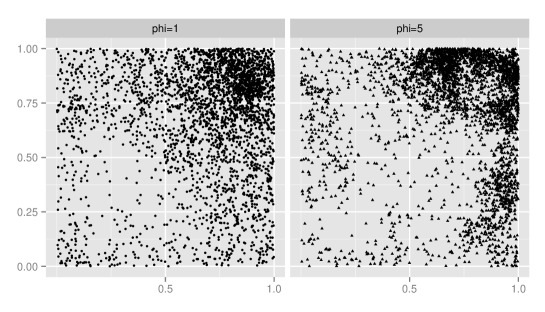
Figure 1: The plot of univariate LGCP: $\phi=1$ (left) and $\phi=5$ (right)

The numbers of simulated points for the cases are (1) $n=3,185$ and (2) $n=3,400$, respectively. As our prior choice, we assume $\beta_{0},\beta_{1},\beta_{2}\sim\mathcal{N}(0,100)$ and a flat prior with sufficiently large support for $\phi$. For the AMP approach, we discard first $i_{0}=1,000$ samples as the burn-in period and preserve subsequent $I=5,000$ samples as posterior samples. As for the choice of $N_{imp}$, we set $N_{imp}=1,000$. We implement adaptive random walk MH, algorithm 4 in Andrieu and Thoms (2008) for updating $\bm{\theta}$. As benchmark cases, we implement an elliptical slice sampling algorithm and MMALA with a grid approximated likelihood. Detailed fitting for both algorithms is explained in the Appendix. We set $K=2,500$. For elliptical slice sampling and MMALA, we discard the first $i_{0}=10,000$ samples as burn-in and retain the subsequent $I=100,000$ samples as posterior draws.

We consider different settings for $(M,N_{B})$: (i) (400, 9), (ii) (400, 1) (iii) (100, 36) and (iv) (100, 4). For (i) and (iii), $(M,N_{B})$ are chosen so that $M\times N_{B}=3,600$. For (ii) and (iv), $(M,N_{B})$ are selected so that $M\times N_{B}=400$. Case (i) provides a setting where $M$ is relatively large and $N_{B}$ is also taken large enough for accurate moments evaluation. Case (ii) provides a setting where $M$ is relatively large and $N_{B}$ is taken too small for accurate moments evaluation. Similarly, case (iii) yields relatively small grids and fine moments evaluation while case (iv) offers a situation where both approximation are coarse.

Tables 1 and 2 show the estimation results. For both datasets, the AMP approach shows much smaller values of the inefficiency factor (IF) than elliptical slice sampling and MMALA. The inefficiency factor is the ratio of the numerical variance of the estimate from the MCMC samples relative to that from hypothetical uncorrelated samples, and is defined as $1+2\sum_{t=1}^{\infty}\rho_{t}$ where $\rho_{t}$ is the sample autocorrelation at lag $t$. It suggests the relative number of correlated draws necessary to attain the same variance of the posterior sample mean from the uncorrelated draws (e.g., Chib (2001)). The results suggest that the AMP approach is more efficient than elliptical slice sampling and MMALA.

Table 1: Estimation results for simulated point patterns: $\phi=1$

	True	Mean	Stdev	$95\%$ Int	IF	Mean	Stdev	$95\%$ Int	IF
		Elliptical				MMALA
$\beta_{0}$	6	5.974	0.548	[4.788, 6.800]	6382	6.232	0.474	[5.370, 7.176]	6087
$\beta_{1}$	3	2.490	0.477	[1.682, 3.419]	3830	2.404	0.677	[0.827, 3.520]	4950
$\beta_{2}$	3	3.076	0.876	[1.480, 4.903]	5963	2.527	0.764	[1.164, 3.790]	5810
$\sigma^{2}$	1	0.796	0.654	[0.236, 2.718]	2175	0.630	0.561	[0.204, 2.413]	3139
$\phi$	1	2.319	1.408	[0.422, 5.458]	2846	2.991	1.719	[0.415, 6.755]	3033
$\sigma^{2}\phi$	1	1.203	0.240	[0.807, 1.727]	1733	1.214	0.277	[0.763, 1.871]	1133
		AMP (i)				AMP (ii)
$\beta_{0}$	6	6.721	0.973	[5.034, 9.098]	18	6.778	1.059	[5.065, 9.291]	19
$\beta_{1}$	3	1.887	0.913	[0.041, 3.691]	11	1.946	0.873	[0.237, 3.631]	13
$\beta_{2}$	3	2.230	0.902	[0.303, 3.993]	18	2.328	0.921	[0.403, 3.978]	15
$\sigma^{2}$	1	1.075	0.828	[0.257, 3.419]	20	1.165	0.910	[0.241, 3.554]	18
$\phi$	1	1.934	1.484	[0.347, 5.829]	32	1.402	1.088	[0.271, 4.487]	28
$\sigma^{2}\phi$	1	1.252	0.301	[0.770, 1.956]	20	0.968	0.205	[0.620, 1.391]	19
		AMP (iii)				AMP (iv)
$\beta_{0}$	6	6.505	0.905	[4.948, 8.632]	24	6.582	0.965	[4.677, 8.784]	39
$\beta_{1}$	3	2.110	0.864	[0.334, 3.768]	18	2.061	0.887	[0.397, 3.917]	13
$\beta_{2}$	3	2.261	0.843	[0.648, 3.910]	28	2.351	0.869	[0.576, 4.178]	14
$\sigma^{2}$	1	1.002	0.827	[0.215, 3.406]	20	1.038	0.844	[0.222, 3.304]	17
$\phi$	1	1.899	1.606	[0.285, 6.430]	28	1.899	1.606	[0.285, 6.430]	28
$\sigma^{2}\phi$	1	1.110	0.330	[0.642, 1.999]	20	0.951	0.224	[0.565, 1.434]	29

Across the different $(M,N_{B})$ choices, the estimation results for the AMP with $(M,N_{B})=(400,9)$ are closer to those of elliptical slice sampling and MMALA than other AMP fits. The posterior density of $\sigma^{2}\phi$ for AMP with $(M,N_{B})=(400,1)$ shows some bias for the rough surface case. Although AMP with $(M,N_{B})=(100,36)$ and $(M,N_{B})=(100,1)$ recovers the true values, the posterior distributions are flatter, especially for the rough surface cases, than with $(M,N_{B})=(400,9)$. Although elliptical slice sampling and MMALA with $K=2,500$ fails to recover $\sigma^{2}\phi$ for the case of $\phi=5$, AMP with the exception of $(M,N_{B})=(400,1)$ recover the all true values. This suggests that $K=2,500$ is not enough for exact posterior sampling for this case. Comparing the different $N_{B}$, small $N_{B}$ reduce the posterior variance of $\sigma^{2}\phi$. Especially, for the rough surface case, although AMP with $(M,N_{B})=(400,1)$ shows the shorter credible interval (CI) for $\sigma^{2}\phi$ than with $(M,N_{B})=(400,9)$, this CI doesn’t include the true value. Likewise, for the $M=100$ cases, although AMP with $(M,N_{B})=(100,4)$ recovers the true parameter value, this reflects its larger posterior variance than $M=400$ cases. In AMP approach, $M$ controls the posterior variance because $M$ can be considerd as ”number of responses” and $N_{B}$ controls the biases for the posterior estimator and its variance because insufficient $N_{B}$ causes the biases in the moments calculations.

Table 2: Estimation results for simulated point patterns: $\phi=5$. Bold denotes that $95\%$ credible interval does not include the true value.

	True	Mean	Stdev	$95\%$ Int	IF	Mean	Stdev	$95\%$ Int	IF
		Elliptical				MMALA
$\beta_{0}$	6	5.591	0.403	[4.789, 6.328]	4013	5.706	0.844	[4.286, 7.214]	6777
$\beta_{1}$	3	3.637	0.512	[2.693, 4.475]	3491	3.916	1.059	[1.540, 5.549]	6331
$\beta_{2}$	3	3.174	0.683	[1.953, 4.743]	4693	2.694	0.956	[1.024, 4.207]	6335
$\sigma^{2}$	1	0.814	0.323	[0.455, 1.724]	2734	0.945	0.467	[0.432, 2.281]	3455
$\phi$	5	5.087	1.896	[1.897, 8.943]	3260	4.619	2.015	[1.346, 9.875]	4165
$\sigma^{2}\phi$	5	3.641	0.538	[2.712, 4.863]	2392	3.622	0.515	[2.757, 4.795]	1096
		AMP (i)				AMP (ii)
$\beta_{0}$	6	6.010	0.732	[4.653, 7.690]	11	6.337	1.168	[4.426, 9.155]	36
$\beta_{1}$	3	3.576	1.073	[1.351, 5.716]	14	3.440	1.247	[1.116, 5.926]	17
$\beta_{2}$	3	2.479	1.140	[0.025, 4.512]	14	2.203	1.244	[-0.473, 4.632]	21
$\sigma^{2}$	1	1.037	0.514	[0.499, 2.517]	22	1.319	0.836	[0.486, 3.535]	41
$\phi$	5	5.166	2.197	[1.429, 10.13]	17	2.736	1.467	[0.663, 6.556]	33
$\sigma^{2}\phi$	5	4.504	0.847	[2.994, 6.304]	15	2.683	0.432	[1.934, 3.640]	21
		AMP (iii)				AMP (iv)
$\beta_{0}$	6	5.899	0.800	[4.628, 7.790]	14	5.968	0.919	[4.514, 8.418]	50
$\beta_{1}$	3	3.710	1.143	[1.231, 5.903]	14	3.852	1.141	[1.597, 6.071]	17
$\beta_{2}$	3	2.725	1.145	[0.144, 4.810]	36	2.671	1.228	[-0.118, 4.862]	12
$\sigma^{2}$	1	1.108	0.501	[0.566, 2.546]	49	1.151	0.634	[0.498, 2.865]	24
$\phi$	5	5.297	2.448	[1.475, 10.53]	36	4.219	2.126	[1.167, 9.230]	44
$\sigma^{2}\phi$	5	4.996	1.394	[3.005, 8.582]	21	3.914	0.997	[2.380, 6.369]	45

Wider credible intervals are also reported in Filippone and Girolami (2014). The posterior distributions of the parameters with MCMC based algorithms including elliptical slice sampling are sharply peaked and highly dependent on the sampled GP (Murray and Adams (2010) and Filippone and Girolami (2014)). Since the estimation results of MMALA show high IFs which are close to elliptical slice sampling, we may not have reached convergence to the stationary distribution for both MMALA and elliptical slice sampling.

Overall, the estimation results suggest that even if $M$ is of moderate dimension, the AMP approach recovers the posterior distribution as long as $N_{B}$ is fine enough. Also, the AMP approach with sufficiently large $M$ and $N_{B}$ captures the true values even in the rough surface case where finer resolution (larger $K$) over the study region is required.

Table 3: Computational Efficiency for the simulated data

Method	Time	IF	(Time/$I$)	(Time/$I$)$\times$IF
	(sec)	(min, max)	(sec)	(min, max)
$\phi=1$
Elliptical	324446	(1133, 6087)	2.94	(3341, 17953)
MMALA	347672	(1733, 6382)	3.16	(5477, 20171)
AMP (i)	15748	(11, 32)	3.14	(34.5, 100)
AMP (ii)	11780	(13, 28)	2.35	(30.6, 65.9)
AMP (iii)	4360	(18, 28)	0.87	(15.6, 24.4)
AMP (iv)	815	(13, 39)	0.16	(2.1, 6.3)
$\phi=5$
Elliptical	329205	(2392, 4693)	2.99	(7158, 14045)
MMALA	347933	(1096, 6777)	3.16	(3466, 21435)
AMP (i)	16086	(11, 22)	3.21	(35.3, 70.6)
AMP (ii)	11221	(17, 41)	2.24	(38.1, 92.0)
AMP (iii)	4717	(14, 49)	0.94	(13.2, 46.2)
AMP (iv)	855	(12, 50)	0.17	(2.0, 8.5)

Comparing the efficiency of algorithms is difficult. Here, we focus on comparing the computational efficiency of elliptical slice sampling, MMALA and AMP approach. We use the ”(computational time for one iteration (Time/$I$)) $\times$ (Inefficiency Factor)”, which corresponds to the approximate time for generating one independent sample from the stationary distribution. The AMP approach is implemented without parallelization of calculation of moments, so the results for the AMP approach are conservative. Table 3 shows the computational efficiency of each approach. ”Time” means the computational time (seconds) for generating $I$ posterior samples (we ignore the burn-in period here). We show the minimum and maximum of inefficiency factor for parameters in Table 1 and 2. Overall, AMP approaches are far faster than elliptical slice sampling and MMALA approaches. For AMP approaches, even with $(M=400,N_{B}=9)$, at most 100 seconds is required for generating one independent approximate posterior samples. Finally, the IF factors may be helpful but, due to dependence on how the actual computing environments were configured for the different approaches, it is difficult to attempt to meaningfully compare run times. As for the comparison of the performance of INLA and MCMC based approach for a spatial LGCP, Taylor and Diggle (2014) compare the predictive accuracy of MCMC and INLA for a spatial LGCP with fixed parameters values. In this setting, they found that MCMC provides more accurate estimates of predictive probabilities than INLA approach with 100,000 iterations. However, only comparing the estimation accuracy may not be enough because it ignores the rapid computation that INLA provides.

4.2 A multivariate LGCP

As a second example, we consider a mLGCP (M$\o$ller et al. (1998)), a three dimensional LGCP. This model introduces larger hyperparameter dimensionality than the univariate LGCP. MCMC based inferences for this model are difficult due to their huge computational costs. So, in this example and the real data application in the next section, we focus only on implementation of AMP approach without elliptical slice sampling and MMALA. In fact, we implement a model similar to that for the tree species dataset in the next section and the parameter settings are based on the real data application described in section 5. The simulation model is defined as

$$\begin{aligned} \bm{\lambda}(\bm{s})&=\exp\biggl{(}\bm{1}_{3}\beta_{0}+\mathbf{\Gamma}\bm{\nu}(\bm{s})\biggl{)},\\ \bm{\nu}_{i}(\mathcal{S})&\sim\mathcal{N}(\bm{0},\mathbf{C}_{\phi_{i}}(\mathcal{S},\mathcal{S}))\end{aligned}\quad\begin{aligned} \mathbf{\Gamma}=\begin{pmatrix}2&0&0\\ -1&1&0\\ 1&0&1\end{pmatrix},\quad\bm{\nu}(\bm{s})=\begin{pmatrix}\nu_{1}(\bm{s})\\ \nu_{2}(\bm{s})\\ \nu_{3}(\bm{s})\\ \end{pmatrix},\end{aligned}$$ (21)

where $\bm{\nu}_{i}$ is independent zero mean and unit variance GP with isotropic exponential correlation function having decay parameters $\phi_{i}$, respectively. The correlation between the first and corresponding rows is introduced from the latent process $\nu_{1}$ and individual behavior is captured by $\nu_{2}$ and $\nu_{3}$. When $\gamma_{i1}$ and $\gamma_{j1}$ have different signs, the $i$-th and $j$-th point patterns show negative dependence, i.e, the cross pair correlation function is smaller than 1 (e.g., M$\o$ller et al. (1998) and Illian et al. (2008)). The number of simulated points for each component is $N_{1}=639$, $N_{2}=1,050$ and $N_{3}=1,283$. Figure 2 shows the three jointly simulated point patterns. The negative dependence between first and second point pattern is observed, which is induced by the $\gamma_{21}=-1$. We set $M=144$, $N_{B}=25$ and $N_{imp}=1,000$.

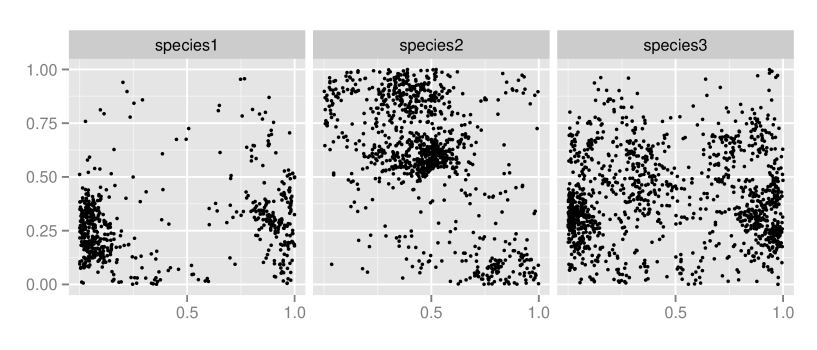
Figure 2: The plot of the simulated three dimensional LGCP

We assume $\beta_{0}\sim\mathcal{N}(0,100)$, $\gamma_{ij}^{2}\sim\mathcal{G}(2,1)$ and a flat prior with sufficiently large support for $\phi_{i}$. Due to the lack of identifiability for the variance parameter and the decay parameter in the GP (Zhang (2004)), we put a relatively informative prior on the components of $\mathbf{\Gamma}$, $(\gamma_{ij})_{i,j=1,2,3}$. The burn in period is $i_{0}=1,000$ and $I=5,000$ samples are preserved as posterior samples. As in the univariate LGCP, we implement adaptive random walk MH, algorithm 4 in Andrieu and Thoms (2008) for parameter estimation. The computational cost of the AMP approach is $\mathcal{O}((3M)^{3})$ for implementing Laplace approximation. Table 3 shows the estimation results for the data. Our approach recovers parameter values well with small inefficiency factors. The posterior variances for $\phi_{2}$ and $\phi_{3}$ are larger than for $\phi_{1}$.

Table 4: Estimation results for the simulated three dimensional LGCP

	True	Mean	Stdev	$95\%$ Int	IF
AMP $(M,N_{B})=(144,25)$
$\beta_{0}$	7	7.200	0.491	[6.353, 8.295]	24
$\phi_{1}$	3	3.056	1.001	[1.582, 5.497]	21
$\phi_{2}$	5	3.540	1.793	[1.118, 7.576]	24
$\phi_{3}$	5	3.659	1.978	[1.105, 8.518]	26
$\gamma_{11}$	2	1.933	0.231	[1.519, 2.413]	11
$\gamma_{21}$	-1	-1.130	0.246	[-1.676, -0.688]	19
$\gamma_{31}$	1	1.192	0.218	[0.795, 1.629]	42
$\gamma_{22}$	1	1.335	0.280	[0.929, 2.074]	8
$\gamma_{33}$	1	1.109	0.247	[0.752, 1.710]	27

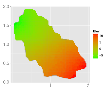
Figure 3: The plot of demeaned surface of elevation

5 Application

In this section, we implement our approach for a real dataset. Our overall dataset consists of tree locations in Duke Forest, comprising 63 species, a total of 14,992 individuals with recorded location. We select 3 prevalent species yielding relatively large number of points: (i). acer rubrum (acru, Red Maple), (ii). frangula caroliniana (frca, Carolina Buckthorn) and (iii). liquidambar styraciflua (list, Sweetgum), and embed the study region $\mathcal{D}$ onto $[0,2]\times[0,2]$. The numbers of points in each pattern are $N_{1}=1,251$, $N_{2}=1,120$ and $N_{3}=1,067$, respectively. Again, we consider the mLGCP as discussed in example 2 of the simulation studies. As a covariate, we include demeaned elevation (elevation) for each point, its surface is in figure 3. Figure 4 shows the observed point patterns. Negative dependence between acru and frca is expected from the figure.

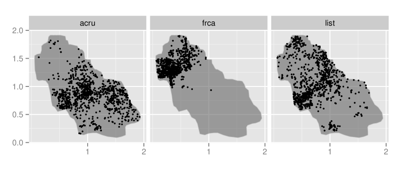
Figure 4: The plot of point patterns of three species in Duke forest: 1. Red Maple (left), 2. Carolina Buckthorn (middle) and 3. Sweetgum (right)

We consider a three dimensional LGCP, i.e., $\bm{\lambda}(\bm{s})=\exp\biggl{(}\bm{1}_{3}\beta_{0}+\mathbf{X}(\bm{s})\bm{\beta}_{1}+\mathbf{\Gamma}\bm{\nu}(\bm{s})\biggl{)}$ where $\mathbf{X}$ is a 3$\times 3$ matrix whose $i$-th diagonal element is elevation_i and for $i=1,2,3$. We assume the same specification for $\mathbf{\Gamma}$ and $\bm{\nu}(\bm{s})$ in Section 4.2. We also estimate an independent three dimensional LGCP, i.e., $\gamma_{21}=\gamma_{31}=0$, with our AMP approach. We discard $i_{0}=1,000$ samples as burn-in period and preserve $I=5,000$ samples as posterior samples. For the grid selection, at first, we take an $80\times 80$ regular grid over $[0,2]\times[0,2]$, and preserve the grid points inside $\mathcal{D}$. The total number of grid points inside $\mathcal{D}$ is $K=3,052$. Then, we construct larger blocks so that $M=120$, i.e., we aggregate about 25 blocks for each larger block. $N_{B}$ is dependent on each aggregated block, i.e., $N_{B_{m}}\approx 25$ for $m=1,\ldots,M$. We set $N_{imp}=1,000$. Again, we implement an adaptive random walk MH, algorithm 4 in Andrieu and Thoms (2008). The prior specification is $\bm{\beta}=(\beta_{0},\bm{\beta}_{1})\sim N(\bm{0},100\mathbf{I}_{4})$, $\gamma_{ij}^{2}\sim\mathcal{G}(2,1)$ and flat priors for the $\phi_{i}$ with large support.

Table 5 shows the estimation results. The estimated value of $\gamma_{21}$ is negative implying that acru and frca are negatively correlated as Figure 4 suggested. The inefficiency factors for the parameters with the AMP approach are small. The result for a independent LGCP model shows smaller variance for $\phi_{2}$ and $\phi_{3}$ than that for the dependent LGCP. The effect of elevation is different among species, significantly negative except for acru.

Table 5: Estimation results for Duke forest dataset: AMP for independent mLGCP (left) and for dependent mLGCP (right)

	AMP-Ind					AMP-Dep
	Mean	Stdev	$95\%$ Int	IF		Mean	Stdev	$95\%$ Int	IF
$\beta_{0}$	5.953	0.430	[4.949, 6.773]	17		5.728	0.472	[4.848, 6.704]	45
$\beta_{1,1}$	0.085	0.095	[-0.095, 0.259]	13		0.094	0.116	[-0.124, 0.325]	33
$\beta_{1,2}$	-0.618	0.211	[-1.056, -0.253]	13		-0.606	0.166	[-0.951, -0.290]	20
$\beta_{1,3}$	-0.188	0.074	[-0.338, -0.058]	21		-0.191	0.078	[-0.354, -0.020]	22
$\phi_{1}$	3.156	1.167	[1.190, 5.846]	39		1.798	0.776	[0.740, 3.682]	14
$\phi_{2}$	2.594	0.967	[0.972, 4.803]	22		5.335	3.232	[1.535, 12.47]	29
$\phi_{3}$	4.159	1.367	[1.869, 7.135]	37		6.202	2.513	[2.143, 11.37]	22
$\gamma_{11}$	1.616	0.272	[1.230, 2.235]	52		1.883	0.326	[1.355, 2.614]	26
$\gamma_{22}$	2.313	0.324	[1.747, 2.957]	28		1.858	0.355	[1.269, 2.652]	51
$\gamma_{33}$	1.452	0.193	[1.127, 1.890]	36		1.135	0.170	[0.852, 1.567]	57
$\gamma_{21}$						-1.083	0.364	[-1.737, -0.361]	19
$\gamma_{31}$						1.093	0.277	[0.597, 1.640]	16

6 Brief discussion

We proposed a two stage model fitting approach for univariate and multivariate LGCPs which is based on developing an approximate marginal posterior (AMP) distribution for the model parameters. Through the simulation studies, we demonstrated that our approach recovers the true parameter values even with relatively low dimensional grids. Furthermore, the results suggest that the AMP approach is applicable for mLGCP models, which introduce many more parameters than the univariate case. Comparison with the two competitive approaches - elliptical slice sampling and MMALA - suggest improved efficiency for AMP in the univariate case. Elliptical slice sampling and MMALA become computationally infeasible for the multivariate case. The AMP computational scheme is similar to INLA in spirit, but INLA might not be well-suited to the multivariate case. The AMP approach also obtains sample based joint posterior distribution $\bm{z}$, which enable us to estimate nonlinear or joint posterior probability of $\bm{z}$. In fact, given posterior $\bm{\theta}$s, we can sample $\bm{z}|\mathcal{S}$ efficiently in a parallel computation scheme with elliptical slice sampling or MALA without the fine tuning.

Appendix

A: MCMC based Posterior Sampling for LGCP

In fitting the LGCP model, we have a stochastic integral of the form $\int_{\mathcal{D}}\lambda(\bm{u}|\bm{\theta},z(\bm{u})d\bm{u}$ in the exponential of the likelihood. We use grid cell approximation for this integral as well as for the product term in the likelihood yielding

$$\mathcal{L}(\mathcal{S}|\bm{\theta},\bm{z})=\exp\biggl{(}|D|-\sum_{k=1}^{K}\lambda(\bm{u}_{k}|\bm{\theta},z(\bm{u}_{k}))\Delta_{k}\biggl{)}\prod_{k=1}^{K}\lambda(\bm{u}_{k}|\bm{\theta},z(\bm{u}_{k}))^{n_{k}}\quad\bm{u}_{1},\ldots,\bm{u}_{K}\in\mathcal{D}$$ (22)

where $n_{k}$ is the number of events in grid $k$, $K$ is the number of grid cells, $n=\sum_{k=1}^{K}n_{k}$ is the total number of points in the point pattern, $\bm{u}_{k}$ is the centroid of the $k$-th grid cell and $\Delta_{k}$ is the area of $k$-th grid. Although fitting this approximation is straightforward because we only require evaluation of $\lambda(\bm{u}_{k}|\bm{\theta},z(\bm{u}_{k}))$ over the grid cells, sampling of a $K$ dimensional vector from a GP would be a computational burden. We consider two types of MCMC based sampling strategies for the GP.

One approach is the manifold Metropolis adjusted Langevin algorithm (MMALA, Girolami and Calderhead (2011)) for the LGCP. Girolami and Calderhead (2011) implement MMALA for the simulated LGCP and show its computational efficiency for sampling of a GP relative to standard MALA with fixed $\bm{\beta}$ and $\bm{\zeta}$ at true values. Diggle et al. (2013) and Taylor et al. (2015) modify the implementation of MMALA in Girolami and Calderhead (2011) for a LGCP with sampling $\bm{\beta}$ and $\bm{\zeta}$. We basically follow the discussion in Diggle et al. (2013) and Taylor et al. (2015). We assume

$$\log\lambda(\bm{s}|\bm{\theta},z(\bm{s})) =\bm{X}(\bm{s})\bm{\beta}+z(\bm{s}),\quad\bm{z}(\mathcal{S})\sim\mathcal{N}(\bm{0},\mathbf{C}_{\bm{\zeta}}(\mathcal{S},\mathcal{S}))\quad\bm{s}\in\mathcal{D}$$ (23)

$$\bm{z} =\mathbf{L}_{\bm{\zeta}}\bm{\nu},\quad\mathbf{L}_{\bm{\zeta}}\mathbf{L}_{\bm{\zeta}}^{{}^{\prime}}=\mathbf{C}_{\bm{\zeta}}$$ (24)

where $\mathbf{L}_{\bm{\zeta}}$ is the Cholesky decomposition of $\mathbf{C}_{\bm{\zeta}}$, $\bm{\theta}=(\bm{\nu},\bm{\beta},\bm{\zeta})$, $\bm{\zeta}$ is the parameter vector for the GP, $\bm{\nu}$ is a zero mean and unit variance normal vector. Diggle et al. (2013) discuss the preconditioning matrix, $\mathbf{M}^{-1}$ (Girolami and Calderhead (2011)), to define the proposal for MMALA.

$$q(\bm{\theta}^{*}|\bm{\theta}^{(i-1)})=\mathcal{N}(\bm{\omega}^{(i-1)},\mathbf{\Omega}^{(i-1)})$$ (25)

where

$$\bm{\omega}^{(i-1)}=\begin{pmatrix}\bm{\nu}^{(i-1)}+\frac{\sigma_{0}^{2}\sigma_{\bm{\nu}}^{2}\mathbf{M}^{-1}_{\bm{\nu}}\partial\log\pi(\bm{\theta}^{(i-1)}|\mathcal{S})/\partial\bm{\nu}}{2}\\ \bm{\beta}^{(i-1)}+\frac{\sigma_{0}^{2}\sigma_{\bm{\beta}}^{2}\mathbf{M}^{-1}_{\bm{\beta}}\partial\log\pi(\bm{\theta}^{(i-1)}|\mathcal{S})/\partial\bm{\beta}}{2}\\ \bm{\zeta}^{(i-1)}\end{pmatrix},\quad\mathbf{\Omega}^{(i-1)}=\sigma_{0}^{2}\begin{pmatrix}\sigma_{\bm{\nu}}^{2}\mathbf{M}^{-1}_{\bm{\nu}}&0&0\\ 0&\sigma_{\bm{\beta}}^{2}\mathbf{M}^{-1}_{\bm{\beta}}&0\\ 0&0&c\sigma_{\bm{\zeta}}^{2}\mathbf{\Sigma}_{\bm{\zeta}}\end{pmatrix}$$ (26)

They set $\sigma_{\bm{\nu}}^{2}=1.65^{2}/\text{dim}(\bm{\nu})^{1/3}$, $\sigma_{\bm{\beta}}^{2}=1.65^{2}/\text{dim}(\bm{\beta})^{1/3}$ and $\sigma_{\bm{\zeta}}^{2}=2.38^{2}/\text{dim}(\bm{\zeta})$. They also set $c=0.4$ and tune $\sigma_{0}^{2}$ adaptively so that the acceptance rate of 0.574 is achieved. Although they consider common $\sigma_{0}^{2}$ and sample all parameters simultaneously, we consider, independently, $\sigma_{0}^{2}$ for $\bm{\nu}$ and $\sigma_{1}^{2}$ for $(\bm{\beta},\bm{\zeta})$ and separately sample $\bm{\nu}$ and $(\bm{\beta},\bm{\zeta})$ to improve mixing. The main computational cost is calculation of $\mathbf{M}^{-1}_{\bm{\nu}}$ for high dimensional $\bm{\nu}$. $\mathbf{M}^{-1}_{\bm{\nu}}$ and $\mathbf{M}^{-1}_{\bm{\beta}}$ are the negative inverse of the Fisher information matrix with respect to $\bm{\nu}$ and $\bm{\beta}$,

$$\mathbf{M}_{\bm{\nu}} =-E_{\bm{y},\bm{\nu}|\bm{\beta},\bm{\zeta}}(\nabla_{\bm{\nu}}\nabla_{\bm{\nu}}\mathcal{L})=\mathbf{L}_{\bm{\zeta}}^{\prime}\mathbf{D}\mathbf{L}_{\bm{\zeta}}+\mathbf{I}$$ (27)

$$\mathbf{M}_{\bm{\beta}} =-E_{\bm{y},\bm{\nu}|\bm{\beta},\bm{\zeta}}(\nabla_{\bm{\beta}}\nabla_{\bm{\beta}}\mathcal{L})=\mathbf{X}^{\prime}\mathbf{D}\mathbf{X}+(1/\kappa_{\bm{\beta}})\mathbf{I}$$ (28)

where $\kappa_{\bm{\beta}}$ is the prior variance for $\bm{\beta}$ and $\mathbf{D}$ is the diagonal matrix whose $(k,k)$ element is $\exp(\bm{X}(\bm{s}_{k})\bm{\beta}+\sigma^{2}/2)\Delta_{k}$.

In practice, calculation of $\mathbf{M}^{-1}_{\bm{\nu}}$ within each MCMC iteration is computationally expensive because $\mathbf{M}^{-1}_{\bm{\nu}}$ is high dimensional and dense. Taylor et al. (2015) consider initial guesses at $\bm{\nu}$ and $\bm{\beta}$ followed by a quadratic approximation to the target. Instead, we calculate the initial guesses of $\mathbf{M}^{-1}_{\bm{\nu}}$ and $\mathbf{M}^{-1}_{\bm{\beta}}$ by a slightly modified strategy. Furthermore, we fix $\mathbf{M}^{-1}_{\bm{\nu}}$ but update $\mathbf{M}^{-1}_{\bm{\beta}}$ within MCMC iteration. Due to the log-concavity of the likelihood, the maximum a posteriori (MAP) estimator is available (M$\o$ller et al. (1998)). We follow the discussion in M$\o$ller et al. (1998) to search for the MAP estimators where $\mathbf{M}^{-1}_{\bm{\nu}}$ and $\mathbf{M}^{-1}_{\bm{\beta}}$ are evaluated at the initial step. At first, since the gradient with respect to $\bm{\zeta}$ is hard to calculate, we fix initial values of $\bm{\zeta}$ at the minimum contrast estimator based on pair correlation function for LGCP by using spatstat package (Baddeley and Turner (2005)). Given the fixed $\bm{\zeta}$, the gradient decent algorithm is available as a mode search for both $\bm{\nu}$ and $\bm{\beta}$ (see, M$\o$ller et al. (1998)), i.e., iterate $\bm{\nu}^{(i)}=\bm{\nu}^{(i-1)}+\delta_{\bm{\nu}}\partial\log\pi(\bm{\theta}^{(i-1)}|\mathcal{S})/\partial\bm{\nu}$ and $\bm{\beta}^{(i)}=\bm{\beta}^{(i-1)}+\delta_{\bm{\beta}}\partial\log\pi(\bm{\theta}^{(i-1)}|\mathcal{S})/\partial\bm{\beta}$ until convergence, where $\delta_{\bm{\nu}}$ and $\delta_{\bm{\beta}}$ are bandwidth parameters. Since the algorithm diverges under large values of bandwidth parameters, we tune $\delta_{\bm{\nu}}$ and $\delta_{\bm{\beta}}$ small enough for each dataset. Calculated initial values (MAP estimator for $(\bm{\nu},\bm{\beta})$ and minimum contrast estimator for $\bm{\zeta}$) of $(\bm{\nu},\bm{\beta},\bm{\zeta})$ are also used in the elliptical slice sampling algorithm.

In addition to MMALA for sampling the GP, we implement elliptical slice sampling (Murray et al. (2010) and Murray and Adams (2010)) as discussed in Leininger and Gelfand (2016) for a spatial LGCP. We sample $\bm{\nu}^{*}=\bm{\nu}\cos(\omega)+\bm{\eta}\sin(\omega)$ where $\bm{\eta}\sim\mathcal{N}(\bm{0},\mathbf{I})$ and $\omega\in[0,2\pi)$ through the elliptical slice sampling algorithm (see, Murray et al. (2010)). As for sampling of $(\bm{\beta},\bm{\zeta})$, we follow the same approach as in MMALA, as explained above.

B: Figures

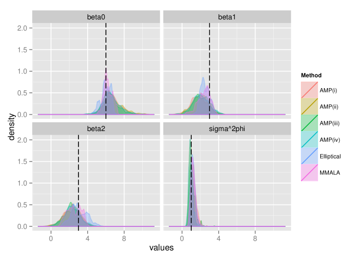
Figure 5: The plot of posterior density for the univariate LGCP: $\phi=1$. Black dashed lines are true values

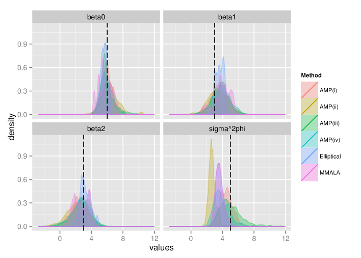
Figure 6: The plot of posterior density for the univariate LGCP: $\phi=5$. Black dashed lines are true values

References

- Aitchison and Ho (1989) Aitchison, J. and C. H. Ho (1989). The multivariate Poisson-log normal distribution. Biometrika 76, 643–653.
- Allard et al. (2001) Allard, D., A. Brix, and J. Chadoeuf (2001). Testing local independence between two point processes. Biometrics 57, 508–517.
- Andrieu and Roberts (2009) Andrieu, C. and G. O. Roberts (2009). The pseudo-marginal approach for efficient Monte Carlo computations. Annals of Statistics 37, 697–725.
- Andrieu and Thoms (2008) Andrieu, C. and J. Thoms (2008). A tutorial on adaptive MCMC. Statistics and Computing 18, 343–373.
- Baddeley and Turner (2005) Baddeley, A. and R. Turner (2005). spatstat: an R package for analyzing spatial point patterns. Journal of Statistical Software 12, 1–42.
- Banerjee et al. (2014) Banerjee, S., B. P. Carlin, and A. E. Gelfand (2014). Hierarchical Modeling and Analysis for Spatial Data, 2nd ed. Chapman and Hall/CRC.
- Banerjee et al. (2008) Banerjee, S., A. E. Gelfand, A. O. Finley, and H. Sang (2008). Gaussain predictive process models for large spatial data sets. Journal of the Royal Statistical Society, Series B 70, 825–848.
- Barndorff-Nielsen and Cox (1989) Barndorff-Nielsen, O. E. and D. R. Cox (1989). Asymptotic Technique for Use in Statistics. Chapman and Hall/CRC.
- Beaumont (2003) Beaumont, M. A. (2003). Estimation of population growth or decline in genetically monitored populations. Genetics 164, 1139–1160.
- Besag (1994) Besag, J. E. (1994). Discusson to the paper: Representations of knowledge in complex systems. by Grenander, U. and M. I. Miller. Journal of the Royal Statistical Society, Series B 56, 549–603.
- Bowers et al. (2004) Bowers, K. J., S. D. Johnson, and K. Pease (2004). Perspective hot-spotting: the future of crime mapping. The British Journal of Criminology 44, 641–658.
- Brix and Diggle (2001) Brix, A. and P. J. Diggle (2001). Spatiotemporal prediction for log-Gaussian Cox processes. Journal of the Royal Statistical Society, Series B 63, 823–841.
- Brix and Mller (2001) Brix, A. and J. Mller (2001). Space-time multi type log Gaussian Cox processes with a view to modelling weeds. Scandinavian Journal of Statistics 28, 471–488.
- Burslem et al. (2001) Burslem, D. F. R. P., N. C. Garwood, and S. C. Thomas (2001). Tropical forest diversity–the plot thickens. Science 291, 606–607.
- Chainey and Ratcliffe (2005) Chainey, S. P. and J. H. Ratcliffe (2005). GIS and Crime Mapping. Wiley.
- Chakraborty et al. (2011) Chakraborty, A., A. E. Gelfand, A. M. Wilson, A. M. Latimer, and J. A. Silander (2011). Point pattern modelling for degraded presence-only data over large regions. Journal of the Royal Statistical Society, Series C 60, 757–776.
- Chib (2001) Chib, S. (2001). Markov chain Monte Carlo methods: computation and inference. In G. Elliott, C. W. J. Granger, and A. Timmermann (Eds.), Handbook of Econometrics, Volume 5, pp. 3569–3649. Amsterdam: North Holland Press.
- Datta et al. (2016) Datta, A., S. Banerjee, A. O. Finley, and A. E. Gelfand (2016). Hierarchical nearest-neighbor Gaussian process models for large geostatistical datasets. Journal of the American Statistical Association 111, 800–812.
- Diggle (2003) Diggle, P. (2003). Statistical Analysis of Spatial Point Patterns, 2nd ed. Hodder Arnold.
- Diggle (2009) Diggle, P. (2009). Discusson to the paper: Approximate Bayesian inference for latent Gaussian models by using integrated nested Laplace approximations. by Rue, H., S. Martino. and N. chopin. Journal of the Royal Statistical Society, Series B 71, 319–392.
- Diggle and Milne (1983) Diggle, P. and R. K. Milne (1983). Bivariate Cox processes: some models for bivariate spatial point patterns. Journal of the Royal Statistical Society, Series B 45, 11–21.
- Diggle et al. (2013) Diggle, P. J., P. Moraga, B. Rowlingson, and B. M. Taylor (2013). Spatial and spatio-temporal log-Gaussian Cox processes: extending the geostatistical paradigm. Statistical Science 28, 542–563.
- Doornik (2007) Doornik, J. (2007). Ox: Object Oriented Matrix Programming. Timberlake Consultants Press.
- Doucet et al. (2015) Doucet, A., M. K. Pitt, G. Deligiannidis, and R. Kohn (2015). Efficient implementation of Markov chain Monte Carlo when using an unbiased likelihood estimator. Biometrika 102, 295–313.
- Filippone and Girolami (2014) Filippone, M. and M. Girolami (2014). Pseudo-marginal Bayesian inference for Gaussian processes. IEEE Transactions on Pattern Analysis and Machine Intelligence 36, 2214–2226.
- Filippone et al. (2013) Filippone, M., M. Zhong, and M. Girolami (2013). A comparative evaluation of stochastic-based inference methods for Gaussian process models. Machine Learning 93, 93–114.
- Genton and Kleiber (2015) Genton, M. G. and W. Kleiber (2015). Cross-covariance functions for multivariate geostatistics. Statistical Science 30, 147–163.
- Girolami and Calderhead (2011) Girolami, M. and B. Calderhead (2011). Riemann manifold Langevin and Hamiltonian Monte Carlo methods. Journal of the Royal Statistical Society, Series B 73, 123–214.
- Grubesic and Mack (2008) Grubesic, T. H. and E. A. Mack (2008). Spatio-temporal interaction of urban crime. Journal Quantitative Criminology 24, 285–306.
- Illian et al. (2008) Illian, J., A. Penttinen, H. Stoyan, and D. Stoyan (2008). Statistical Analysis and Modelling of Spatial Point Patterns. Wiley.
- Illian et al. (2012) Illian, J. B., S. H. Srbye, and H. Rue (2012). A toolbox for fitting complex spatial point process models using integrated nested Laplace approximation (INLA). Annals of Applied Statistics 6, 1499–1530.
- Katzfuss (2016) Katzfuss, M. (2016). A multi-resolution approximation for massive spatial datasets. Journal of the American Statistical Association, forthcoming.
- Leininger and Gelfand (2016) Leininger, T. J. and A. E. Gelfand (2016). Bayesian inference and model assessment for spatial point patterns using posterior predictive samples. Bayesian Analysis. forthcomming.
- Liang et al. (2009) Liang, S., S. Banerjee, and A. E. Gelfand (2009). Bayesian wombling for spatial point processes. Biometrics 65, 1243–1253.
- Lindgren and Rue (2015) Lindgren, F. and H. Rue (2015). Bayesian spatial modelling with R-INLA. Journal of Statistical Software 63, 1–25.
- Lindgren et al. (2011) Lindgren, F., H. Rue, and J. Lindström (2011). An explicit link between Gaussian fields and Gaussian Markov random fields. Journal of the Royal Statistical Society, Series B 73, 423–498.
- Marsan and Lengliné (2008) Marsan, D. and O. Lengliné (2008). Extending earthquakes’ reach through cascading. Science 319, 1076–1079.
- Martins et al. (2013) Martins, T. G., D. Simpson, F. Lindgren, and H. Rue (2013). Bayesian computing with INLA: New features. Computational Statistics and Data Analysis 67, 68–83.
- Minka (2001) Minka, T. P. (2001). Expectation Propagation for approximate Bayesian inference. In Proceedings of the 17th Conference in Uncertainty in Artificial Intelligence, San Francisco. Morgan Kaufmann.
- Mller et al. (1998) Mller, J., A. R. Syversveen, and R. P. Waagepetersen (1998). Log Gaussian Cox processes. Scandinavian Journal of Statistics 25, 451–482.
- Mller and Waagepetersen (2004) Mller, J. and R. Waagepetersen (2004). Statistical Inference and Simulation for Spatial Point Processes. Chapman and Hall/RC.
- Murray and Adams (2010) Murray, I. and R. P. Adams (2010). Slice sampling covariance hyperparameters of latent Gaussian models. In Advances in Neural Information Processing Systems 23, Cambridge, MA. MIT Press.
- Murray et al. (2010) Murray, I., R. P. Adams, and M. M. Graham (2010). Elliptical slice sampling. In Proceedings of the 13th International Conference on Artifical Intelligence and Statistics (AISTAT). AISTAT Press.
- Ogata (1999) Ogata, Y. (1999). Seismicity analysis through point-process modeling: A review. Pure and Applied Geophysics 155, 471–507.
- Paci et al. (2016) Paci, L., M. A. Beamonte, A. E. Gelfand, P. Gargallo, and M. Salvador (2016). Analysis of residential property sales using space-time point patterns. Discussion Paper.
- Picard et al. (2009) Picard, N., A. Bar-Hen, F. Mortier, and J. Chadoeuf (2009). The multi-scale marked area-interaction point process: a model for the spatial pattern of trees. Scandinavian Journal of Statistics 36, 23–41.
- Robert and Casella (2004) Robert, C. P. and G. Casella (2004). Monte Carlo Statistical Methods. Springer-Verlag.
- Roberts and Rosenthal (1998) Roberts, G. O. and J. S. Rosenthal (1998). Optimal scaling of discrete approximations to Langevin diffusions. Journal of the Royal Statistical Society, Series B 60, 255–268.
- Roberts and Stramer (2003) Roberts, G. O. and O. Stramer (2003). Langevin diffusions and Metropolis-Hastings algorithms. Methodology and Computing in Applied Probability 4, 337–358.
- Roberts and Tweedie (1996) Roberts, G. O. and R. L. Tweedie (1996). Exponential convergence of langevin distributions and their discrete approximations. Bernoulli 2, 341–363.
- Rue and Held (2005) Rue, H. and L. Held (2005). Gaussian Markov Random Field: Theory and Applications, volume 104 of Monographs on Statistics and Applied Probability. Chapman and Hall.
- Rue et al. (2009) Rue, H., S. Martino, and N. Chopin (2009). Approximate Bayesian inference for latent Gaussian models by using integrated nested Laplace approximations. Journal of the Royal Statistical Society, Series B 71, 319–392.
- Rue et al. (2016) Rue, H., A. Riebler, S. H. Srbye, J. B. Illian, D. P. Simpson, and F. K. Lindgren (2016). Bayesian computing with INLA: a review. Available at http://arxiv.org/abs/1604.00860.
- Ruiz-Moreno et al. (2010) Ruiz-Moreno, D., M. Pascual, M. Emch, and M. Yunus (2010). Spatial clustering in the spatio-temporal dynamics of endemic cholera. BMC Infectious Diseases, doi:10.1186/1471–2334–10–51.
- Schmidt and Gelfand (2003) Schmidt, A. M. and A. E. Gelfand (2003). A Bayesian coregionalization approach for multivariate pollutant data. Journal of Geophysical Research: Atmospheres 108.
- Simpson et al. (2016) Simpson, D., J. B. Illian, F. Lindgren, S. H. Srbye, and H. Rue (2016). Going off grid: Computationally efficient inference for log-Gaussian Cox processes. Biometrika 73, 49–70.
- Taylor et al. (2015) Taylor, B. M., T. M. Davies, B. S. Rowlingson, and P. J. Diggle (2015). Bayesian inference and data augmentation schemes for spatial, spatiotemporal and multivariate log-Gaussian Cox processes in R. Journal of Statistical Software 63.
- Taylor and Diggle (2014) Taylor, B. M. and P. J. Diggle (2014). INLA or MCMC? A tutorial and comparative evaluation for spatial prediction in log-Gaussian Cox processes. Journal of Statistical Computation and Simulation 84, 2266–2284.
- Tierney and Kadane (1986) Tierney, L. and J. B. Kadane (1986). Accurate approximations for posterior moments and marginal densities. Journal of the American Statistical Association 81, 82–86.
- Waagepetersen (2004) Waagepetersen, R. (2004). Convergence of posteriors for discretized log Gaussin Cox processes. Statistics and Probability Letters 66, 229–235.
- Waagepetersen et al. (2016) Waagepetersen, R., Y. Guan, A. Jalilian, and J. Mateu (2016). Analysis of multispecies point patterns by using multivariate log-Gaussian Cox processes. Journal of the Royal Statistical Society, Series C 65, 77–96.
- Wiegand et al. (2009) Wiegand, T., I. Martínez, and A. Huth (2009). Recruitment in tropical tree species: revealing complex spatial patterns. The American Naturalist 174, 106–140.
- Zhang (2004) Zhang, H. (2004). Inconsistent estimation and asymptotically equal interpolations in model-based geostatistics. Journal of the American Statistical Association 99, 250–261.