Upper limits for Mass and Radius of objects around Proxima Cen from SPHERE/VLT

Abstract

The recent discovery of an earth-like planet around Proxima Centauri has drawn much attention to this star and its environment. We performed a series of observations of Proxima Centauri using SPHERE, the planet finder instrument installed at the ESO Very Large Telescope UT3, using its near infrared modules, IRDIS and IFS. No planet was directly detected but we set upper limits on the mass up to 7 au exploiting the AMES-COND models. Our IFS observations reveal that no planet more massive than $\sim$ 6-7 M_Jup can be present within 1 au. The dual band imaging camera IRDIS also enables us to probe larger separations than the other techniques like the radial velocity or astrometry. We obtained mass limits of the order of 4 M_Jup at separations of 2 au or larger representing the most stringent mass limits at separations larger than 5 au available at the moment. We also did an attempt to estimate the radius of possible planets around Proxima using the reflected light. Since the residual noise for this observations are dominated by photon noise and thermal background, longer exposures in good observing conditions could further improve the achievable contrast limit.

1 Introduction

After the recent discovery of a terrestrial planet around the star Proxima Centauri (Anglada-Escudé et al. 2016) a new interest arose in the nearest star system to the Sun. While this planet, that has a separation of just 0.05 au with a period of 11.2 days and a minimum mass of 1.3 M_⊕, cannot be imaged with the current instrumentation aimed to detect the emitted light from extrasolar planets like e.g. GPI (Macintosh et al. 2006) and SPHERE (Beuzit et al. 2008), it would be however interesting to have informations about further possible objects at larger separations to fully characterize the system. Exploiting direct imaging observations it is possible to put some constraints on the mass and on the radius of other objects in the Proxima system. A similar work has been done in the past exploiting both the radial velocity (RV) technique (Endl & Kürster 2008; Zechmeister et al. 2009; Barnes et al. 2014) and astrometric measurements (Lurie et al. 2014), but never exploiting direct imaging techniques. We repeatedly observed Proxima with SPHERE in the past months with the aim to obtain precise astrometry of a background star which is undergoing a microlensing event caused by the approaching of Proxima (Sahu et al. 2014). This star is clearly visible even when is not undergoing the microlensing effect. This will give a unique opportunity to directly measure the star mass (Zurlo et al., in prep.). However, the same data can be exploited to put some constraints on the mass of possible objects around Proxima after calculating the contrast obtained from these observations.

2 Data and data reduction

Proxima Cen was observed during six different nights as part of the Guaranteed Time Observations (GTO) program of the SPHERE consortium. The observations are listed in Table 1. All the observations were performed in the IRDIFS mode, with the IFS (Claudi et al. 2008) operating at a spectral resolution R=50 in the wavelength range between 0.95 and 1.35 $\mu$m with a field of view (FOV) of 1.7^′′ $\times$1.7^′′ corresponding to a maximum projected separation from the star of$\sim$1 au and IRDIS (Dohlen et al. 2008) operating in the H band with the H23 filter pair (wavelength H2=1.587 $\mu$m; wavelength H3=1.667 $\mu$m; Vigan et al. 2010) with a circular FOV with a radius of $\sim$5^′′ corresponding to a maximum projected separation of $\sim$7 au.

Table 1: SPHERE observations of Proxima Cen. DIT represents the expopsure time for each exposure expressed in seconds, nDIT represents the number of frames for each datacube of the dataset.

Date	Obs. mode	Coronagraph	nDIT;DIT(s) IRDIS	nDIT;DIT(s) IFS	Rot.Ang. (∘)	Seeing (′′)
2015-03-30	IRDIFS	N_ALC_YJH_S	3$\times$12;16	3$\times$12;16	3.12	0.93
2016-01-18	IRDIFS	N_ALC_YJH_S	7$\times$40;16	7$\times$20;32	25.74	2.20
2016-02-17	IRDIFS	N_ALC_YJH_S	11$\times$10;16	11$\times$5;32	13.52	1.86
2016-02-29	IRDIFS	N_ALC_YJH_S	7$\times$30;16	7$\times$15;32	22.56	0.78
2016-03-27	IRDIFS	N_ALC_YJH_S	5$\times$40;16	5$\times$25;32	25.69	2.08
2016-04-15	IRDIFS	N_ALC_YJH_S	6$\times$40;16	6$\times$20;32	28.72	0.62

For both IFS and IRDIS the data reduction was partly performed using the pipeline of the SPHERE data center hosted at OSUG/IPAG in Grenoble. IFS data reduction was performed using the procedure described by Zurlo et al. (2014) and by Mesa et al. (2015) to create calibrated datacubes composed of 39 frames at different wavelengths on which we applied the principal components analysis (PCA; e.g. Soummer et al. 2012; Amara et al. 2015) to reduce the speckle noise. The self-subtraction was appropriately taken into account by injecting in the data fake planets at different separations. An alternative data reduction was performed using the approach described in Vigan et al. (2015) leading to consistent results. IRDIS data were reduced following the procedure described by Zurlo et al. (2016) and applying the PCA algorithm for the reduction of the speckle noise. An alternative reduction was performed following the procedure by Gomez Gonzalez et al. 2016 (submitted) leading to a comparable contrast. For all the dataset the contrast was calculated following the procedure described by Mesa et al. (2015) corrected taking into account the small sample statistics as devised in Mawet et al. (2014).

3 Results

Given the very low galactic latitude of Proxima, several sources were visible in the IRDIS FOV. One example of the reduced images is shown in the left panel of Figure 1. Background stars move rapidly in these images due to the large parallax and proper motion of Proxima, so that they can be very easily identified. One single background source (that is the star undergoing the microlensing event) was visible in the IFS FOV for three observing nights and it is shown on the right panel of Figure 1. However, all the detected sources are background stars not bound with Proxima, so that no reliable companion candidate is detected in the SPHERE images.

Given the quality of the atmospheric conditions with respect to the other nights (see Table 1), the data from the night of 2016-04-15 give the best contrast as shown in Table 2. Exploiting the very good conditions of this night, we were able to obtain a very deep $5\sigma$ contrast. As listed in Table 2, the contrast is better than $10^{-6}$ at a separation of 0.4^′′ using IFS and just above $10^{-6}$ at the same separation using IRDIS. These values are in good agreement with what expected when SPHERE is observing a very bright target (see e.g. Zurlo et al. 2014; Mesa et al. 2015) and is similar to what obtained until now during the SPHERE observations for targets with similar magnitude (see e.g. Vigan et al. 2015). In Figure 2 we display the contrast in magnitude versus the separation expressed in au for both instruments. We can get a contrast better than 15 magnitudes at projected separations larger than 0.5 au with IFS while with IRDIS we obtain a contrast better than 14 magnitudes at the same separation than IFS and we obtain a contrast better than 17 magnitudes at separation larger than of 2.5 au.

Using the theorical model AMES-COND (Allard et al. 2003) we were able to set upper limit on the mass of possible objects around Proxima. For this aim we assumed a distance for Proxima of 1.295 pc (van Leeuwen 2007) and an age of 4.8 $\pm$ 1 Gyr (Thévenin et al. 2002; Bazot et al. 2016). Moreover, we assumed J and H magnitudes of 5.357 and 4.835 (Cutri et al. 2003) respectively for the star. The upper mass limit plots obtained in this way are displayed in Figure 3 as solid lines. We found a mass limit of $\sim$7.5 M_Jup at a separation of 0.2 au and of $\sim$6 M_Jup at separation larger than 0.6 au with IFS. On the other hand, using IRDIS we were able to get a limit of 8 M_Jup at $\sim$0.4 au and lower than 5 M_Jup at separation larger than 2 au. Given the large uncertainties on the age of Proxima, we also calculated the mass limits considering an age of 3.8 and 5.8 Gyr with the aim to show how the mass limits change according to the stellar age and to set a more reliable range of mass limits. These results are shown as dashed lines in Figure 3. In the same Figure we included, as a comparison with our results, the mass limit obtained by Endl & Kürster (2008) using the RV method (shown as red circles) and the limits obtained by Lurie et al. (2014) using astrometric measurements (blue squares).

While the April 2016 data are clearly the best dataset that we obtained, we also combined the data from all the observing epochs attempting to increase the detection capability. This was performed using the procedure described in Vigan et al. (2015) and based on the MESS program (Bonavita et al. 2012) that is able to determine the probability of at least one detection in our observing dates calculated on a grid of values for the semi-major axis and for the companion mass. The results are shown on the left panel of Figure 4. They are in good agreement with the results obtained in Figure 3 but at shorter separations we are able to obtain a better sensitivity as demonstrated by a comparison with the results of the same procedure performed using only the best epoch data dipslayed on the right panel of Figure 4. This demonstrate, for example, that in this second case the 95% of probability of detection is cut at 0.4 au while using all the observations combined we arrive at 0.2 au.

It is also possible to make an estimation of the limit in radius around Proxima assuming planets shining in reflected light.

However, the contribution to the luminosity of the planet in the regime around Proxima should be mainly dominated by the its intrinsic luminosity while the contribution from the reflected light should be less important. For this reason the limits obtained through the reflected light are not very meaningful with values ranging from $\sim$1.5 R_Jup at 0.2 au to $\sim$3 R_Jup at $\sim$1 au and $\sim$10R_Jup at $\sim$7 au. Values of the radius of the order of $\sim$1R_Jup as foreseen from the theorical models are then much more probable for substellar objects around Proxima.

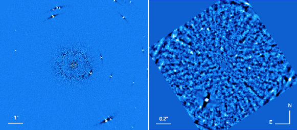
Figure 1: Final images obtained for IRDIS (left) and for IFS (right). The IRDIS image is from 2016-04-15 observation while the IFS image is from 2016-02-29 observation to be able to show the background star that was no more into the IFS FOV in April.

Table 2: SPHERE IFS and IRDIS contrasts at a separation of 0.4^′′ for the different observing nights.

Date	IFS Contrast@0.4′′	IRDIS Contrast@0.4′′
2015-03-30	8.01$\times 10^{-6}$	8.98$\times 10^{-5}$
2016-01-18	5.55$\times 10^{-6}$	1.03$\times 10^{-5}$
2016-02-17	3.82$\times 10^{-6}$	2.30$\times 10^{-5}$
2016-02-29	1.79$\times 10^{-6}$	5.84$\times 10^{-6}$
2016-03-27	3.83$\times 10^{-6}$	7.22$\times 10^{-6}$
2016-04-15	8.58$\times 10^{-7}$	1.84$\times 10^{-6}$

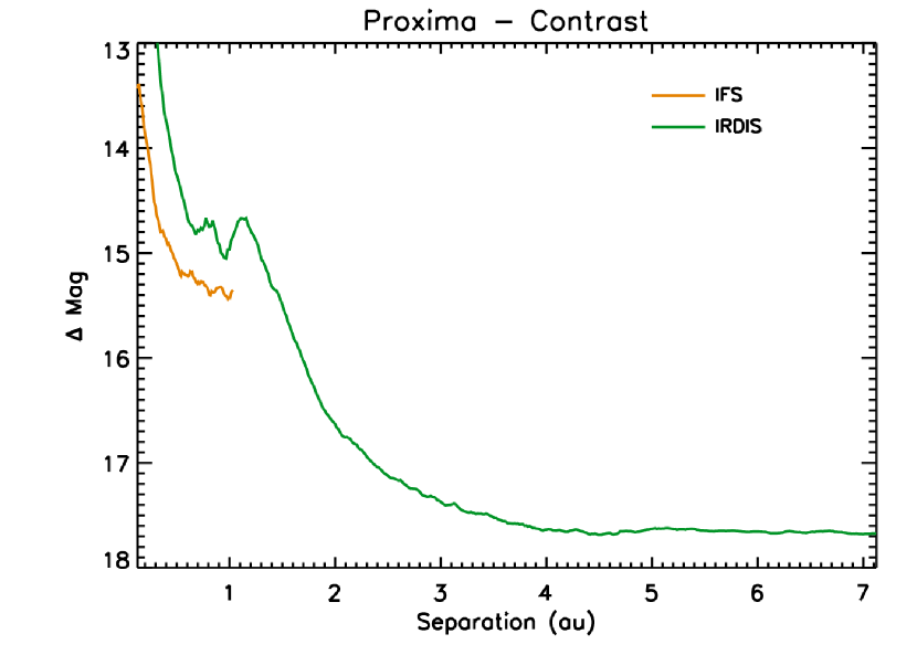
Figure 2: Magnitude contrast plot obtained for Proxima using SPHERE. The orange line represents the contrast using IFS while the green line represents the contrast obtained using IRDIS.

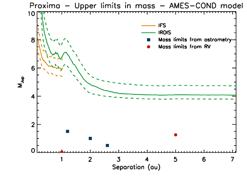
Figure 3: Mass limits for planets around Proxima calculated from the SPHERE contrast using the AMES-COND model. The orange lines represent limits from IFS, the green ones limits from IRDIS. The dashed lines are drawn to take into account the uncertainties on the stellar age. The limits from astrometry (blue squares) and the limits from RV (red circles) are also shown as a comparison with our results.

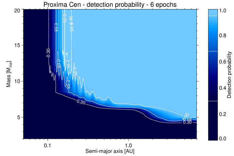
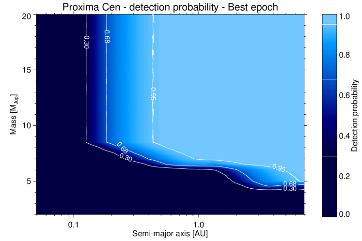
Figure 4: Left Mean probability of at least one detection of a substellar companion around Proxima Cen using the combination of all the observations as function of the companion mass and the semimajor axis. Right Same but using just best epoch data.

4 Discussion and Conclusions

We presented the results of the analysis of the SPHERE data for Proxima Centauri. While it was not possible, as expected, to retrieve any signal from the planet recently discovered with the RV technique by Anglada-Escudé et al. (2016), we were able to set constraints on the mass and on the radius of other possible planets around this star.

Previous works put constraints on the minimum mass through the RV technique. One example is the value of $\sim$15 $M_{\oplus}$ at a separation of 1 au for the minimum mass (M$\sin{i}$) given by Endl & Kürster (2008). Other authors gave similar results. The comparison of these limits with those obtained by direct imaging allows to exclude face-on orbits for possible sub-stellar objects. Extrapolating the results reported by Zechmeister et al. (2009) at larger separations, we can conclude that our results are consistents with those from RV at separation of $\sim$7 au, that is just at the limit of the IRDIS FOV.

Different results were obtained with astrometric measurements. For example, Lurie et al. (2014) set a mass limit of $\sim$ 1.5 M_Jup at 1.2 au, of $\sim$ 1 M_Jup at 2 au and of $\sim$0.5 M_Jup at 2.6 au. These constraints are more sensitive to smaller planets than those that we can obtain with SPHERE. Indeed, we get mass limits of $\sim$7.5 M_Jup at a separation of 0.2 au and of the order of 6 M_Jup at separation between 0.6 and 1 au. However, the wider IRDIS FOV allowed to obtain mass limits at even larger separations where RV and astrometry are less sensitive. We obtained mass limits better than $\sim$4 M_Jup at separations larger than 2 au. It is important to stress that these limits at separations larger then $\sim$5 au concern a region unconstrained so far. Moreover, as pointed out by Dupuy et al. (2011), model-based substellar mass determinations could be overestimated. For this reason the mass limits from direct imaging could be even lower than those determined with our measures.

We also attempted to obtain a limit for the radius using the reflected light. However, the limits that we obtained are not very stringent probably because the intrinsic luminosity is more important than reflected light for objects around Proxima. Limits of $\sim$1R_Jup foreseen through the theoretical models are probably more reliable for these substellar objects around Proxima.

We obtained these results with a total exposure time of $\sim$1 hour. Given that the residual noise from our observation is mainly dominated by the photon noise at separations largere than 0.3^′′ for IFS and at separations larger than 1.5^′′ for IRDIS, we should be able to further improve our contrast with longer exposures taken in sky conditions comparable to those of April 2016 or better. Under these assumptions, we could be able to improve our contrast as the square root of the exposure time ratio. However, this improvement will not be comparable with the sensitivity reached by the other methods reported above. For example, a long exposure of 20 hours taken during more than one night will enable us to reach a contrast of 1.89$\times 10^{-7}$ with IFS corresponding to a mass limit of 4.9 M_Jup at a separation of 0.5^′′, still far from the limits obtained with RV and astrometry. To be able to further improve the mass limit obtained with direct imaging we will have to wait for the availability of future instruments both in space (like e.g. James Webb Space Telescope - JWST) and from ground using future giant segmented mirror telescope like Giant Magellan Telescope (GMT - Johns 2008), the Thirty Meter Telescope (TMT - Nelson & Sanders 2008) and the European Extremely Large Telescope (E-ELT - Gilmozzi & Spyromilio 2007).
Using the online ETC for JWST we have calculated the contrast at different separations in the L^′ band for one hour observation and trasformed it in mass limits using again the AMES-COND models. We synthetized these results in Table 3 from which one can see that we can have a quite good gain especially at larger separation where we can obtain limit similar to those obtained through the RV.

Table 3: Contrast and mass limit for the L^′ band with JWST.

Separation (′′)	Magnitude limits	Mass limits (MJup)
0.5	20.2	5.3
1.0	21.7	3.5
1.5	22.6	2.5
2.0	23.6	1.7
2.5	23.8	1.5

References

- Allard et al. (2003) Allard F., Guillot T., Ludwig H.-G., et al. 2003, in Martín E., ed., Brown Dwarfs Vol. 211 of IAU Symposium, Model Atmospheres and Spectra: The Role of Dust. p. 325
- Amara et al. (2015) Amara A., Quanz S. P., Akeret J., 2015, Astronomy and Computing, 10, 107
- Anglada-Escudé et al. (2016) Anglada-Escudé G., Amado P., Barnes J., et al. 2016, Nature, 536, 437
- Barnes et al. (2014) Barnes J., Jenkins J., Jones H., et al 2014, MNRAS, 439, 3094
- Bazot et al. (2016) Bazot M., Christensen-Dalsgaard J., Gizon L., et al. 2016, MNRAS, 460, 1254
- Beuzit et al. (2008) Beuzit J.-L., Feldt M., Dohlen K., et al. 2008, in Ground-based and Airborne Instrumentation for Astronomy II Vol. 7014 of SPIE, SPHERE: a ’Planet Finder’ instrument for the VLT. p. 701418
- Bonavita et al. (2012) Bonavita M., Chauvin G., Desidera S., Gratton R., Janson M., Beuzit J. L., Kasper M., Mordasini C., 2012, A&A, 537, A67
- Claudi et al. (2008) Claudi R. U., Turatto M., Gratton R. G., et al. 2008, in Society of Photo-Optical Instrumentation Engineers (SPIE) Conference Series Vol. 7014 of SPIE, SPHERE IFS: the spectro differential imager of the VLT for exoplanets search
- Cutri et al. (2003) Cutri R. M., Skrutskie M. F., van Dyk S., et al. 2003, VizieR Online Data Catalog, 2246
- Dohlen et al. (2008) Dohlen K., Langlois M., Saisse M., et al. 2008, in Ground-based and Airborne Instrumentation for Astronomy II Vol. 7014 of SPIE, The infra-red dual imaging and spectrograph for SPHERE: design and performance. p. 70143L
- Dupuy et al. (2011) Dupuy T. J., Liu M. C., Ireland M. J., 2011, in Johns-Krull C., Browning M. K., West A. A., eds, 16th Cambridge Workshop on Cool Stars, Stellar Systems, and the Sun Vol. 448 of Astronomical Society of the Pacific Conference Series, . p. 111
- Endl & Kürster (2008) Endl M., Kürster M., 2008, A&A, 488, 1149
- Gilmozzi & Spyromilio (2007) Gilmozzi R., Spyromilio J., 2007, The Messenger, 127
- Johns (2008) Johns M., 2008, in Extremely Large Telescopes: Which Wavelengths? Retirement Symposium for Arne Ardeberg Vol. 6986 of SPIE, The Giant Magellan Telescope (GMT). p. 698603
- Lurie et al. (2014) Lurie J. C., Henry T. J., Jao W.-C., et al. 2014, AJ, 148, 91
- Macintosh et al. (2006) Macintosh B., Graham J., Palmer D., et al. 2006, in Society of Photo-Optical Instrumentation Engineers (SPIE) Conference Series Vol. 6272 of Society of Photo-Optical Instrumentation Engineers (SPIE) Conference Series, The Gemini Planet Imager
- Mawet et al. (2014) Mawet D., Milli J., Wahhaj Z., Pelat D., Absil O., Delacroix C., Boccaletti A., Kasper M., Kenworthy M., Marois C., Mennesson B., Pueyo L., 2014, ApJ, 792, 97
- Mesa et al. (2015) Mesa D., Gratton R., Zurlo A., et al. 2015, ArXiv e-prints
- Nelson & Sanders (2008) Nelson J., Sanders G. H., 2008, in Ground-based and Airborne Telescopes II Vol. 7012 of SPIE, The status of the Thirty Meter Telescope project. p. 70121A
- Sahu et al. (2014) Sahu K. C., Bond H. E., Anderson J., et al. 2014, ApJ, 782, 89
- Soummer et al. (2012) Soummer R., Pueyo L., Larkin J., 2012, ApJL, 755, L28
- Thévenin et al. (2002) Thévenin F., Provost J., Morel P., et al. 2002, A&A, 392, L9
- van Leeuwen (2007) van Leeuwen F., 2007, A&A, 474, 653
- Vigan et al. (2015) Vigan A., Gry C., Salter G., et al. 2015, MNRAS, 454, 129
- Vigan et al. (2010) Vigan A., Moutou C., Langlois M., et al. 2010, MNRAS, 407, 71
- Zechmeister et al. (2009) Zechmeister M., Kürster M., Endl M., 2009, A&A, 505, 859
- Zurlo et al. (2016) Zurlo A., Vigan A., Galicher R., et al. 2016, A&A, 587, A57
- Zurlo et al. (2014) Zurlo A., Vigan A., Mesa D., et al. 2014, A&A, 572, A85