SCHAUDER ESTIMATES FOR EQUATIONS WITH CONE METRICS, I

Bin Guo and Jian Song

ABSTRACT.  This is the first paper in a series to develop a linear and nonlinear theory for elliptic and parabolic equations on Kähler varieties with mild singularities. Donaldson has established a Schauder estimate for linear and complex Monge-Ampère equations when the background Kähler metrics on $\mathbb{C}^{n}$ have cone singularities along a smooth complex hypersurface. We prove a sharp pointwise Schauder estimate for linear elliptic and parabolic equations on $\mathbb{C}^{n}$ with background metric $g_{\beta}=\sqrt{-1}(dz_{1}\wedge d\bar{z_{1}}+\ldots+\beta^{2}|z_{n}|^{-2(1-\beta)}dz_{n}\wedge d\bar{z_{n}})$ for $\beta\in(0,1)$. Our results give an effective elliptic Schauder estimate of Donaldson and a direct proof for the short time existence of the conical Kähler-Ricci flow.

1. Introduction

In [32], Yau considers complex Monge-Ampère equations with a singular right hand side as a generalization of his solution to the Calabi conjecture. More precisely, let $(X,\omega)$ be an $n$-dimensional Kähler manifold with a Kähler form $\omega=\sqrt{-1}\sum g_{i\bar{j}}dz_{i}\wedge d\overline{z_{j}}$ associated to a Kähler metric $g$. Let $L$ and $L^{\prime}$ be two holomorphic line bundles over $X$ equipped with two smooth hermitian metrics $h$ and $h^{\prime}$. Let $\sigma$ and $\sigma^{\prime}$ be two holomorphic sections of $L$ and $L^{\prime}$ respectively. Then various global and local regularity results are established in [32] for solutions of the following complex Monge-Ampère equation with suitable assumptions on $\beta,\beta^{\prime}>0$,

(1.1) $$(\omega+\sqrt{-1}\partial\overline{\partial}\varphi)^{n}=|\sigma|_{h}^{-2\beta}|\sigma^{\prime}|_{h^{\prime}}^{2\beta^{\prime}}e^{F}\omega^{n},$$

where $F\in C^{\infty}(X)$. A fundamental result of Kolodziej [15] shows that as long as $|\sigma|^{-2\beta}|\sigma^{\prime}|^{2\beta^{\prime}}e^{F}\in L^{p}(X)$ for some $p>1$, there exists a unique solution $\varphi\in L^{\infty}(X)\cap PSH(X,\omega)$, where $PSH(X,\omega)$ is the set of all quasi-plurisubharmonic functions on $X$ associated to $\omega$. When $\beta^{\prime}=0$ and $D=\{\sigma=0\}$ is a smooth complex hypersurface of $X$, equation (1.1) becomes

(1.2) $$(\omega+\sqrt{-1}\partial\overline{\partial}\varphi)^{n}=|\sigma|_{h}^{-2\beta}e^{F}\omega^{n}.$$

Equation (1.2) is considered by Donaldson [9] to obtain Kähler-Einstein metrics with cone singularities along the smooth divisor $D$. The curvature equation for $\omega_{\varphi}=\omega+\sqrt{-1}\partial\overline{\partial}\varphi$ from equation (1.2) is given by

$$Ric(\omega_{\varphi})=\left(Ric(\omega)-\sqrt{-1}\partial\overline{\partial}F-\beta Ric(h)\right)+\beta[D],$$

where $[D]$ is the nonnegative current defined by $[D]=\sqrt{-1}\partial\overline{\partial}\log|\sigma|^{2}$. By combining results from [9, 5], $\omega_{\varphi}$ is smooth on $X\setminus D$ and it is equivalent to the standard cone singularities in the conical Hölder sense. In fact, conical Einstein metrics were already studied with potential geometric applications in many literatures (cf. [28, 30, 17, 18]). The recent success in solving the Yau-Tian-Donaldson conjecture (cf. [27, 4, 5, 6, 29]) has also inspired many works on the study of canonical Kähler metrics with cone singularities and their relation to algebraic geometry (cf. [1, 13, 25, 7, 14, 19, 21, 33, 34, 10]). One of the main difficulties in solving (1.2) is how to derive a suitable Schauder estimate for the linearized equation of (1.2). Such an important estimate is first established by Donaldson in [9] with the classical approach of potential theory. Symmetry plays an essential role in the proof and it seems difficult to adapt this approach to more general settings of singular background metrics, in particular, Kähler metrics with cone singularities along divisors of simple normal crossings.

The Schauder estimates for Laplace equations and heat equations are fundamental tools in both PDEs theories and geometric analysis. Apart from the classical potential theory, various proofs have been established by different important analytic techniques (cf. [2, 3, 24, 22, 23, 31]). Recently, an elementary and elegant pointwise Schauder estimate for the standard Laplace equation on $\mathbb{R}^{n}$ is obtained by Wang [31]. Wang’s techniques are quite flexible and we are able to combine such perturbation techniques with geometric gradient estimates to prove sharp Schauder estimates for Laplace equations on $\mathbb{C}^{n}$ with a conical background Kähler metric.

Let $g_{\beta}$ be the standard conical Kähler metric on $\mathbb{C}^{n}$ defined by

$$g_{\beta}=\sqrt{-1}(dz_{1}\wedge d\overline{z_{1}}+\ldots+dz_{n-1}\wedge d\overline{z_{n-1}}+\beta^{2}|z_{n}|^{-2(1-\beta)}dz_{n}\wedge d\overline{z_{n}}),$$

for some $\beta\in(0,1)$, where $z=(z_{1},...,z_{n})$ are the standard complex coordinates on $\mathbb{C}^{n}$. Let

$$\mathcal{S}=\{z_{n}=0\}$$

be the singular set of $g_{\beta}$. Obviously $g_{\beta}$ is a smooth flat Kähler metric on $\mathbb{C}^{n}\setminus\mathcal{S}$ and it extends to a conical Kähler metric on $\mathbb{C}^{n}$ with cone angle $2\pi\beta$ along the hyperplane $\mathcal{S}$.

In this paper, we will consider the following conical Laplace equation with the background conical Kähler metric $g_{\beta}$ on $\mathbb{C}^{n}$

(1.3) $$\Delta_{\beta}u=f,\quad\text{in }~{}B_{\beta}(0,1),$$

where $B_{\beta}(p,r)$ is the geodesic ball in $(\mathbb{C}^{n},g_{\beta})$ centered at $p$ of radius $r$, and

$$\Delta_{\beta}=\sum_{i,j=1}^{n}(g_{\beta})^{i\bar{j}}\frac{\partial^{2}}{\partial z_{i}\partial\overline{z_{j}}}$$

is the Laplace operator associated to $g_{\beta}$. We introduce a family of first order differential operators which are already considered in [9].

Definition 1.1.

We write

$$z_{i}=s_{2i-1}+\sqrt{-1}s_{2i}$$

in real coordinates for $i=1,...,n-1$ and

$$r_{n}=|z_{n}|^{\beta},~{}~{}\theta_{n}=\arg z_{n}.$$

in weighted polar coordinates. The differential operators $D_{j}$ for $j=1,...,2n$ are defined by

$$D_{i}=\frac{\partial}{\partial s_{i}},~{}i=1,2,...,2n-2.$$

and

$$D_{2n-1}=\frac{\partial}{\partial r_{n}},~{}~{}~{}~{}D_{2n}=\frac{\partial}{r_{n}\partial\theta_{n}}.$$

We now state the main result of the paper.

Theorem 1.1.

Suppose $\beta\in(1/2,1)$ and $f(x)$ is Dini continuous on $B_{\beta}(0,1)$ with respect to $g_{\beta}$ for some $\beta\in(0,1)$. Let

$$\omega(r)=\sup_{d_{\beta}(z,w)<r,~{}z,w\in B_{\beta}(0,1)}|f(z)-f(w)|.$$

If $u\in C^{2}(B_{\beta}(0,1)\setminus\mathcal{S})\cap L^{\infty}(B_{\beta}(0,1))$ is a solution of the conical Laplace equation (1.3)

$$\Delta_{\beta}u=f,$$

then there exists $C=C(n,\beta)>0$ such that for any $p,q\in B_{\beta}(0,\frac{1}{2})\setminus\mathcal{S}$,

(1.4) $$\begin{split}&\sum_{i,j=1}^{2n-2}\left|D_{i}D_{j}u(p)-D_{i}D_{j}u(q)\right|+\left|\left(|z_{n}|^{2-2\beta}\frac{\partial^{2}u}{\partial z_{n}\partial\overline{z_{n}}}\right)(p)-\left(|z_{n}|^{2-2\beta}\frac{\partial^{2}u}{\partial z_{n}\partial\overline{z_{n}}}\right)(q)\right|\\ \leq&C\left(d\sup_{B_{\beta}(0,1)}|u|+\int_{0}^{d}\frac{\omega(r)}{r}dr+d\int_{d}^{1}\frac{\omega(r)}{r^{2}}dr\right)\end{split}$$

and

(1.5) $$\begin{split}&\sum_{i=2n-1}^{2n}\sum_{j=1}^{2n-2}\left|D_{i}D_{j}u(p)-D_{i}D_{j}u(q)\right|\\ \leq&C\left(d^{\frac{1}{\beta}-1}\sup_{B_{\beta}(0,1)}|u|+\int_{0}^{d}\frac{\omega(r)}{r}dr+d^{\frac{1}{\beta}-1}\int_{d}^{1}\frac{\omega(r)}{r^{1/\beta}}dr\right),\end{split}$$

where $d=d_{\beta}(p,q)$ is the distance between $p$ and $q$ with respect to $g_{\beta}$.

The estimate (1.4) measures the Hölder continuity of second derivatives of the solution $u$ in the tangential directions of $\mathcal{S}$, while the estimate (1.5) measures Hölder continuity of mixed second derivatives in the tangential and transversal directions. The mixed derivative estimates are more difficult to handle. The case of $\beta\in(0,1/2]$ can be treated in the same fashion and is relatively easy with stronger estimates (c.f. Proposition 2.5).

The conical Hölder function spaces $C_{\beta}^{2,\alpha}$ (cf. Defintion 2.1) for the background Kähler metric $g_{\beta}$ is first introduced in [9]. It is also shown in [9] that if $u\in C_{\beta}^{2,\alpha}(B_{\beta}(0,1))$ for some $\alpha\in\left(0,\min\{\frac{1}{\beta}-1,1\}\right)$ and $\Delta_{\beta}u=f$, then

(1.6) $$||u||_{C_{\beta}^{2,\alpha}(B_{\beta}(0,1/2))}\leq C(n,\beta,\alpha)\left(||u||_{C_{\beta}^{0,\alpha}(B_{\beta}(0,1))}+||f||_{C_{\beta}^{0,\alpha}(B_{\beta}(0,1))}\right).$$

As a direct consequence of Theorem 1.1, we derive the following sharp Schauder estimate, generalizing the Schauder estimate for the Laplace equation on Euclidean $\mathbb{R}^{n}$ and improving Donaldson’s Schauder estimate (1.6).

Corollary 1.1.

Suppose $\beta\in(1/2,1)$ and $f(x)\in C_{\beta}^{0,\alpha}(B_{\beta}(0,1))$ for some $\alpha\in\left(0,\min\{\frac{1}{\beta}-1,1\}\right)$. If $u\in C^{2}(B_{\beta}(0,1)\setminus\mathcal{S})\cap L^{\infty}(B_{\beta}(0,1))$ is a solution of the conical Laplace equation (1.3), then $u\in C_{\beta}^{2,\alpha}(B_{\beta}(0,\frac{1}{2}))$ and

(1.7) $$||u||_{C_{\beta}^{2,\alpha}(B_{\beta}(0,\frac{1}{2}))}\leq C(n,\beta)\left(||u||_{L^{\infty}(B_{\beta}(0,1))}+\frac{||f||_{C_{\beta}^{0,\alpha}(B_{\beta}(0,1))}}{\alpha\left(\min\{\frac{1}{\beta}-1,1\}-\alpha\right)}\right).$$

The Schauder estimate (1.7) improves Donaldson’s original Schauder estimate in the way that it gives the sharp dependence on $\alpha$ for fixed $\beta$ and $u$ is only required to be bounded and locally $C^{2}$. Such dependence on $\alpha$ is a slight modification of the classical Schauder estimates for the standard Laplace equation on $\mathbb{R}^{n}$. In section 2, we will present formulae generalizing estimates (1.4) and (1.5). In particular, the dependance of the constant $C(n,\beta)$ in estimate (1.5) on $\beta$ can be explicitly formulated from the proof of Theorem 1.1.

Our method can be easily modified to derive a Schauder estimate for linear parabolic equations on $\mathbb{C}^{n}$ with the conical background Kähler metric $g_{\beta}$. In section 3, we apply similar techniques to derive sharp Schauder estimates for linear parabolic equations with conical singularities. We first define the parabolic metric ball $\mathcal{Q}_{\beta}(P_{0},r)$ centered at $P_{0}=(p_{0},t_{0})$ of radius $r$ by

$$\mathcal{Q}_{\beta}(P_{0},r)=\{(p,t)\in\mathbb{C}^{n}\times[0,\infty)~{}|~{}d_{\mathcal{P},\beta}((p,t),(p_{0},t_{0}))<r,~{}t<t_{0}\},$$

where

$$d_{\mathcal{P},\beta}((p,t),(p_{0},t_{0}))=\max\{d_{\beta}(p,p_{0}),\sqrt{|t-t_{0}|}\}$$

is the conical parabolic distance on $\mathbb{C}^{n}\times\mathbb{R}$. Denote

$$\mathcal{S}_{\mathcal{P}}=\{(p,t)~{}|~{}p\in\mathcal{S},~{}t\in[0,\infty)\}.$$

We now consider the following conical heat equation with respect to the background conical metric $g_{\beta}$,

(1.8) $$\Box_{\beta}u=f,~{}~{}\textnormal{~{}~{}~{}}~{}\mathcal{Q}_{\beta}((0,1),1),$$

where $\Box_{\beta}=\left(\frac{\partial}{\partial t}-\Delta_{\beta}\right)u$. The following theorem is the parabolic analogue of Theorem 1.1 for the pointwise Schauder estimate for solutions of the conical heat equation (1.8).

Theorem 1.2.

Suppose $f(x,t)$ is Dini continuous on $\mathcal{Q}_{\beta}((0,1),1)$ with respect to $d_{\mathcal{P},\beta}$ for some $\beta\in(1/2,1)$ and let

$$\omega(r)=\sup_{d_{\mathcal{P},\beta}((p_{1},t_{1}),(p_{2},t_{2}))<r,~{}(p_{1},t_{1}),(p_{2},t_{2})\in\mathcal{Q}_{\beta}((0,1),1)}|f(p_{1},t_{1})-f(p_{2},t_{2})|.$$

If $u\in\mathcal{P}^{2}(\mathcal{Q}_{\beta}((0,1),1)\setminus\mathcal{S}_{\mathcal{P}})\cap L^{\infty}(\mathcal{Q}_{\beta}((0,1),1))$ is a solution of the conical heat equation (1.8), then there exists $C(n,\beta)>0$ such that for any $P,Q\in\mathcal{Q}_{\beta}((0,1),\frac{1}{2})\setminus\mathcal{S}_{\mathcal{P}}$,

$$\sum_{i,j=1}^{2n-2}\left|D_{i}D_{j}u(P)-D_{i}D_{j}u(Q)\right|+\left|\left(|z_{n}|^{2-2\beta}\frac{\partial^{2}u}{\partial z_{n}\partial\overline{z_{n}}}\right)(P)-\left(|z_{n}|^{2-2\beta}\frac{\partial^{2}u}{\partial z_{n}\partial\overline{z_{n}}}\right)(Q)\right|$$

$$\leq C\left(d\sup_{B_{\beta}(0,1)}|u|+\int_{0}^{d}\frac{\omega(r)}{r}dr+d\int_{d}^{1}\frac{\omega(r)}{r^{2}}dr\right)$$

and

$$\sum_{i=2n-1}^{2n}\sum_{j=1}^{2n-2}\left|D_{i}D_{j}u(P)-D_{i}D_{j}u(Q)\right|$$

$$\leq C\left(d^{\frac{1}{\beta}-1}\sup_{B_{\beta}(0,1)}|u|+\int_{0}^{d}\frac{\omega(r)}{r}dr+d^{\frac{1}{\beta}-1}\int_{d}^{1}\frac{\omega(r)}{r^{1/\beta}}dr\right),$$

where $d=d_{\mathcal{P},\beta}(P,Q)$.

Similarly like Corollary 1.1, we have the following parabolic Schauder estimates.

Corollary 1.2.

Suppose $\beta\in(1/2,1)$ and $f\in\mathcal{P}_{\beta}^{0,\alpha}(\mathcal{Q}_{\beta}(0,1))$ for some $\alpha\in\left(0,\min\{\frac{1}{\beta}-1,1\}\right)$. If $u\in\mathcal{P}^{2}(\mathcal{Q}_{\beta}((0,1),1)\setminus\mathcal{S})\cap L^{\infty}(\mathcal{Q}_{\beta}((0,1),1))$ is a solution of the conical heat equation (1.8), then $u\in\mathcal{P}_{\beta}^{2,\alpha}(\mathcal{Q}_{\beta}((0,1),\frac{1}{2}))$ and

$$\|u\|_{\mathcal{P}_{\beta}^{2,\alpha}(\mathcal{Q}_{\beta}((0,1),\frac{1}{2}))}\leq C(n,\beta)\Big{(}\sup_{\mathcal{Q}_{\beta}((0,1),1)}|u|+\frac{||f||_{\mathcal{P}_{\beta}^{0,\alpha}(\mathcal{Q}_{\beta}((0,1),1))}}{\alpha\left(\min\{\frac{1}{\beta}-1,1\}-\alpha\right)}\Big{)},$$

where the $\mathcal{P}^{2,\alpha}_{\beta}$-norm and $\mathcal{P}^{0,\alpha}_{\beta}$-norm of functions are defined in Definition 3.1.

In [7], a parabolic Schauder estimate is derived by adapting the elliptic Schauder estimates in [9] and such an estimate leads to the short time existence of the Kähler-Ricci flow on a Kähler manifold with conical singularities along a smooth divisor. The argument in [7] is very long and based on asymptotic analysis for the heat kernel. Our approach is more direct and can be used for more general settings. In the sequel, we will prove the maximal time existence for the conical Kähler-Ricci flow on a Kähler manifold with cone singularities along divisors of simple normal crossings.

In the sequels, we will build the Schauder theory for Laplace and complex Monge-Ampère equations with a background Kähler metric with asymptotically cone singularities based on the techniques developed in this paper. A special case will be the Laplace equation of a background Kähler metric with conical singularities along divisors of simple normal crossings. Furthermore, we are interested in the more degenerate case when the cone angles are allowed to be greater than $2\pi$ or equivalently $\beta>1$. Ultimately, we aim to develop a foundational theory to study analytic and geometric regularity for canonical Kähler metrics on Kähler varieties with mild singularities, in particular, Kähler-Einstein metrics on projective varieties with log terminal singularities. This might lead to deep understanding for the classification of Kähler varieties and algebraic singularities through singular canonical Kähler metrics.

2. Elliptic Schauder estimates

We will prove Theorem 1.1 and Corollary 1.1 in this section.

2.1. Notations

Let $g_{\beta}$ be the standard cone metric on $\mathbb{C}^{n}=\mathbb{C}^{n-1}\times\mathbb{C}$ for some $\beta\in(0,1)$, given by

$$g_{\beta}=\sum_{j=1}^{n-1}\sqrt{-1}dz_{j}\wedge d\overline{z_{j}}+\beta^{2}|z_{n}|^{-2(1-\beta)}\sqrt{-1}dz_{n}\wedge d\overline{z_{n}}.$$

It has conical singularities along the hyperplane

$$\mathcal{S}=\mathbb{C}^{n-1}\times\{0\}$$

with cone angle $2\pi\beta\in(0,2\pi)$. In the following we will also use $\{s_{1},\ldots,s_{2n-2}\}$ to be the real coordinates functions of $\mathbb{C}^{n-1}=\mathbb{R}^{2n-2}$, where $z_{i}=s_{2i-1}+\sqrt{-1}s_{2i}$, for $i=1,...,2n-2$.

We will denote $B_{\beta}(p,r)$ by the open metric ball with respect to $g_{\beta}$ centered at $p\in\mathbb{C}^{n}$ and of radius $r>0$. Let $d_{\beta}(x,y)$ be the distance of $x,~{}y$ with respect to the metric $g_{\beta}$. Since $\beta\in(0,1)$, the smooth part of $(\mathbb{C}^{n},g_{\beta})$ is geodesic convex. More precisely, if $x,y\notin\mathcal{S}$, the minimal geodesic joining $x$ and $y$ does not intersect $\mathcal{S}$.

Definition 2.1.

We define the $C_{\beta}^{0,\alpha}$-norm of a function $u$ on the ball $B_{\beta}(0,1)$ as

$$\|u\|_{C_{\beta}^{0,\alpha}(B_{\beta}(0,1))}=\|u\|_{C^{0}(B_{\beta}(0,1))}+\sup_{x\neq y\in B_{\beta}(0,1)}\frac{|u(x)-u(y)|}{d_{\beta}(x,y)^{\alpha}},$$

for $\alpha\in(0,1]$.

The following definition coincides with the Schauder norm introduced by Donaldson [9].

Definition 2.2.

We define the $C_{\beta}^{2,\alpha}$-norm of a function $u$ on the ball $B_{\beta}(0,1)$ as

$$\begin{split}\|u\|_{C_{\beta}^{2,\alpha}(B_{\beta}(0,1))}=&\|u\|_{C^{0}(B_{\beta}(0,1))}+\sum_{i=1}^{2n}\|D_{i}u\|_{C^{0}(B_{\beta}(0,1))}\\ &+\sum_{i=1}^{2n}\sum_{j=1}^{2n-2}\|D_{i}D_{j}u\|_{C_{\beta}^{0,\alpha}(B_{\beta}(0,1))}+\big{\|}|z_{n}|^{2-2\beta}\frac{\partial^{2}u}{\partial z_{n}\partial\overline{z_{n}}}\big{\|}_{C_{\beta}^{0,\alpha}(B_{\beta}(0,1))}\end{split}$$

for $\alpha\in(0,1]$, where $D_{i}$ is defined in Definition 1.1 for $i=1,2,...,2n$.

Definition 2.3.

We decompose the gradient operator $\nabla_{g_{\beta}}$ by $\nabla_{g_{\beta}}=(D^{\prime},D^{\prime\prime})$, where $D^{\prime}$ and $D^{\prime\prime}$ are given by

$$D^{\prime}=(D_{1},D_{2},...,D_{2n-2}),\quad D^{\prime\prime}=(D_{2n-1},D_{2n}).$$

Obviously, $D^{\prime}$ commute with $D^{\prime\prime}$ and $\Delta_{\beta}$.

2.2. The maximum priniciple

Let $u\in C^{2}(B_{\beta}(0,1)\backslash\mathcal{S})\cap C^{0}(\overline{B_{\beta}(0,1)})$ be a solution to the conical Laplace equation

(2.1) $$\Delta_{\beta}u=\sum_{j=1}^{n-1}\frac{\partial^{2}u}{\partial z_{j}\partial\bar{z}_{j}}+\beta^{-2}|z_{n}|^{2(1-\beta)}\frac{\partial^{2}u}{\partial z_{n}\partial\bar{z}_{n}}=0,\quad\text{in }B_{\beta}(0,1)\backslash\mathcal{S}.$$

Then we have the following maximum principle.

Lemma 2.1.

Suppose $u\in C^{0}(\overline{B_{\beta}(0,1)})\cap C^{2}(B_{\beta}(0,1)\backslash\mathcal{S})$ solves the equation (2.1), then

$$\inf_{\partial B_{\beta}(0,1)}u\leq\inf_{B_{\beta}(0,1)}u\leq\sup_{B_{\beta}(0,1)}u\leq\sup_{\partial B_{\beta}(0,1)}u.$$

Proof.

We first define $u_{\epsilon}(z)=u(z)+\epsilon\log|z_{n}|^{2}$ for any $\epsilon>0$. Since $u$ is continuous on $\overline{B_{\beta}(0,1)}$ and $u_{\epsilon}(z)\to-\infty$ as $z\to\mathcal{S}$, the maximum of $u_{\epsilon}$ in $\overline{B_{\beta}(0,1)}$ cannot be achieved at $\mathcal{S}\cap\overline{B_{\beta}(0,1)}$. Hence the standard maximum principle implies that the supremum of $u_{\epsilon}$ has to be obtained at $\partial B_{\beta}(0,1)\backslash\mathcal{S}$, that is, for any fixed $z\in B_{\beta}(0,1)\backslash\mathcal{S}$,

$$u_{\epsilon}(z)\leq\sup_{\partial B_{\beta}(0,1)}u_{\epsilon}\leq\sup_{\partial B_{\beta}(0,1)}u.$$

Letting $\epsilon\to 0$, we have $u(z)\leq\sup_{\partial B_{\beta}(0,1)}u$ and so $\sup_{B_{\beta}(0,1)}u\leq\sup_{\partial B_{\beta}(0,1)}u$. Similarly we can prove $\inf_{B_{\beta}(0,1)}u\geq\inf_{\partial B_{\beta}(0,1)}u$. ∎

Lemma 2.1 immediately implies uniqueness of the solution in $C^{0}(\overline{B_{\beta}(0,1)})\cap C^{2}(B_{\beta}(0,1)\backslash\mathcal{S})$ to the conical Dirichilet problem

(2.2) $$\left\{\begin{aligned} &\Delta_{\beta}u=0,&\text{in }B_{\beta}(0,1)\backslash\mathcal{S}\\ &u=\varphi\in C^{0}(\partial B_{\beta}(0,1)),&\text{on }\partial B_{\beta}(0,1)\\ \end{aligned}\right.$$

We will establish the existence of the solution to (2.2) in section 2.4.

2.3. One dimensional case

In this section, we establish some basic estimates for the conical Poisson equation on $\mathbb{C}$. Let

$$\hat{g}_{\beta}=\sqrt{-1}|z|^{-2(1-\beta)}dz\wedge d\bar{z}$$

be a conical metric on $\mathbb{C}$ for some $\beta\in(1/2,1)$. We will consider the case when $\beta\in(1/2,1)$ because the case of $\beta\in(0,1/2]$ is relatively easy and can be treated with little modification.

Let $B=B(0,1)\subset\mathbb{C}$ be the Euclidean unit ball. We consider the following conical Poisson equation

(2.3) $$\Delta_{\hat{g}_{\beta}}u=|z|^{2(1-\beta)}\frac{\partial^{2}u}{\partial z\partial\bar{z}}=F,$$

for some continuous function $F\in C^{0}(\overline{B})$.

Suppose $u\in C^{0}(\overline{B})\cap C^{2}(B\backslash\{0\})$ solves equation (2.3). We will apply the Riez representation formula. Let $h$ be the harmonic function satisfying

$$\frac{\partial^{2}}{\partial z\partial\bar{z}}h=0\quad\text{in }B,\quad h|_{\partial B}=u|_{\partial B}.$$

The standard gradient estimate for harmonic functions gives

(2.4) $$\sup_{\frac{1}{2}B}\Big{|}\frac{\partial h}{\partial z}\Big{|}\leq C\|u\|_{L^{\infty}}.$$

The Riesz representation formula ([12]) implies that

(2.5) $$u(z)=h(z)+\frac{1}{2\pi}\int_{|w|<1}\left(\log\frac{|w-z|}{|1-\overline{w}z|}\right)\frac{F(w)}{|w|^{2(1-\beta)}}\sqrt{-1}dw\wedge d\overline{w}.$$

Lemma 2.2.

There exist constants $C_{1}$ and $C_{2}=C_{2}(\beta)>0$ such that

$$\sup_{\frac{1}{2}B^{*}}\Big{|}\frac{\partial u}{\partial z}(z)\Big{|}\leq C_{1}\|u\|_{L^{\infty}(B)}+C_{2}(\beta)\|F\|_{L^{\infty}(B)}.$$

Proof.

We fix $z\in\frac{1}{2}B^{*}$. It follows from (2.5) by direct calculations that

$$\Big{|}\frac{\partial u}{\partial z}\Big{|}\leq\Big{|}\frac{\partial h}{\partial z}\Big{|}+\frac{\sqrt{-1}}{4\pi}\int_{B}\frac{|F(w)|dw\wedge d\overline{w}}{|w-z||w|^{2(1-\beta)}}+\frac{\sqrt{-1}}{4\pi}\int_{B}\frac{|w||F(w)|dw\wedge d\overline{w}}{|1-\overline{w}z||w|^{2(1-\beta)}}.$$

The last term on RHS is bounded by

$$\frac{\sqrt{-1}}{2}\int_{B}\frac{|w||F(w)|dw\wedge d\overline{w}}{|1-\overline{w}z||w|^{2(1-\beta)}}\leq C\|F\|_{\infty}\int_{0}^{1}\frac{t^{2}}{t^{2(1-\beta)}}dt=\frac{C\|F\|_{L^{\infty}(B)}}{2\beta+1}.$$

To estimate the second term on RHS, we divide $B$ into four regions,

$$\Omega_{1}=\left\{w\in B~{}\left|~{}|w|\leq\frac{|z|}{2}\right.\right\},\quad\Omega_{2}=\left\{w\in B~{}\left|~{}|w|\leq|w-z|,|w|\geq\frac{|z|}{2}\right.\right\}$$

$$\Omega_{3}=\left\{w\in B~{}\left|~{}|w-z|\leq\frac{|z|}{2}\leq|w|\right.\right\},\quad\Omega_{4}=\left\{w\in B~{}\left|~{}|w-z|\leq|w|,~{}|w-z|\geq\frac{|z|}{2}\right.\right\}.$$

We have the following estimates

$$\begin{split}\int_{\Omega_{1}}\frac{\sqrt{-1}dw\wedge d\overline{w}}{|w-z||w|^{2(1-\beta)}}\leq\frac{2}{|z|}\int_{|w|\leq\frac{|z|}{2}}\frac{\sqrt{-1}dw\wedge d\overline{w}}{|w|^{2(1-\beta)}}\leq C(\beta)|z|^{2\beta-1},\end{split}$$

$$\begin{split}\int_{\Omega_{2}}\frac{\sqrt{-1}dw\wedge d\overline{w}}{|w-z||w|^{2(1-\beta)}}\leq\int_{\Omega_{2}}\frac{\sqrt{-1}dw\wedge d\overline{w}}{|w|^{2(1-\beta)+1}}\leq C\int_{{|z|/}{2}}^{1}t^{-2(1-\beta)}dt\leq C(\beta),\end{split}$$

$$\begin{split}\int_{\Omega_{3}}\frac{\sqrt{-1}dw\wedge d\overline{w}}{|w-z||w|^{2(1-\beta)}}\leq\frac{C}{|z|^{2(1-\beta)}}\int_{|w-z|\leq\frac{|z|}{2}}\frac{\sqrt{-1}dw\wedge d\overline{w}}{|w-z|}\leq{C}|z|^{2\beta-1},\end{split}$$

$$\begin{split}\int_{\Omega_{4}}\frac{\sqrt{-1}dw\wedge d\overline{w}}{|w-z||w|^{2(1-\beta)}}\leq\int_{\Omega_{4}}\frac{\sqrt{-1}dw\wedge d\overline{w}}{|w-z|^{2(1-\beta)+1}}\leq C\int_{{|z|/2}{}}^{1}t^{-2(1-\beta)}dt\leq C(\beta).\end{split}$$

Combining the above estimates with the gradient estimate (2.4) of $h$, we obtain the desired estimate. We further remark that the constant $C(\beta)$ is comparable to ${1}/({2\beta-1})$.

∎

We now state the main result in this subsection, which is a scaling version of Lemma 2.2.

Proposition 2.1.

Let $u\in C^{0}(\overline{B(0,1)})\cap C^{2}(B(0,1)\backslash\{0\})$ be a solution of equation (2.3) on $B(0,1)$ for some $\beta\in(1/2,1)$. There exists $C=C(n,\beta)>0$ such that for all $\rho\in(0,1)$,

$$\sup_{B(0,\rho/2)\setminus\{0\}}\left|\frac{\partial u}{\partial z}\right|\leq C\left(\frac{||u||_{L^{\infty}(B(0,\rho))}}{\rho}+\rho^{2\beta-1}||F||_{L^{\infty}(B(0,\rho))}\right),$$

where $B(0,\rho)$ is the Euclidean ball in $\mathbb{C}$ centered at $0$ of radius $\rho$.

Proof.

The proposition follows from Lemma 2.2 by scaling the equation and $B(0,\rho)$.

∎

2.4. Conical harmonic functions

In this subsection we will prove that the equation (2.2) admits a unique solution and we will also derive a gradient estimate.

We will construct a solution to the equation (2.2) by smooth approximation. Let $g_{\epsilon}$ be a sequence of smooth Kähler metrics defined by

(2.6) $$g_{\epsilon}=\sqrt{-1}\Big{(}\sum_{j=1}^{n-1}dz_{j}\wedge d\bar{z}_{j}+\beta^{2}(|z_{n}|^{2}+\epsilon)^{-(1-\beta)}dz_{n}\wedge d\bar{z}_{n}\Big{)}.$$

For fixed $r>0$,

$$B_{g_{\epsilon}}(0,0.9r)\subset B_{\beta}(0,r)\subset B_{g_{\epsilon}}(0,r)$$

for sufficiently small $\epsilon>0$.

We consider the following approximating Dirichlet problem

(2.7) $$\left\{\begin{aligned} \Delta_{g_{\epsilon}}u_{\epsilon}=0,&\quad\text{in }B_{\beta}(0,r)\backslash\mathcal{S},\\ u_{\epsilon}=\varphi,&\quad\text{on }\partial B_{\beta}(0,r)\end{aligned}\right.$$

for some $\varphi\in C^{0}(\partial B_{\beta}(0,r))$.

Lemma 2.3.

For any $\epsilon>0$, there exists a unique solution $u_{\epsilon}\in C^{0}(\overline{B_{\beta}(0,r)})\cap C^{\infty}(B_{\beta}(0,r))$ to the conical Dirichlet problem (2.7). Furthermore,

(2.8) $$||u_{\epsilon}||_{L^{\infty}(B_{\beta}(0,r)}\leq\sup_{\partial B_{\beta}(0,r)}|\varphi|.$$

Proof.

Equation (2.7) can be solved by Peron’s method since $g_{\epsilon}$ is a smooth Riemannian metric and the boundary $B_{\beta}(0,r)$ admits admissible barrier functions. Such barrier functions are also constructed in the proof of Lemma 2.5. The estimate (2.8) follows immediately from the maximum principle.

∎

Lemma 2.4.

There exist $C=C(n)$ and $\epsilon_{0}=\epsilon(n,r)>0$ such that for all $0<\epsilon<\epsilon_{0}$,

(2.9) $$\sup_{B_{\beta}(0,r/2)}|\nabla_{g_{\epsilon}}u_{\epsilon}|_{g_{\epsilon}}\leq\frac{C}{r}\mathrm{osc}_{B_{\beta}(0,r)}u_{\epsilon}.$$

Proof.

We will apply Cheng-Yau’s gradient estimates to prove the lemma. We first observe that

$$\mathrm{Ric}(g_{\epsilon})=-\sqrt{-1}\partial\overline{\partial}\log\det g_{\epsilon}=\sqrt{-1}\partial\overline{\partial}\log(|z_{n}|^{2}+\epsilon)^{1-\beta}\geq 0.$$

By Cheng-Yau’s gradient estimate [8], we immediately have

$$\sup_{B_{\beta}(0,r/2)}\Big{(}\sum_{i=1}^{2n-2}\Big{(}\frac{\partial u_{\epsilon}}{\partial s_{i}}\Big{)}^{2}+(|z_{n}|^{2}+\epsilon)^{1-\beta}\Big{|}\frac{\partial u_{\epsilon}}{\partial z_{n}}\Big{|}^{2}\Big{)}=\sup_{B_{\beta}(0,r/2)}|\nabla u_{\epsilon}|^{2}_{g_{\epsilon}}\leq C(n)\frac{(\mathrm{osc}_{B_{\beta}(0,r)}u)^{2}}{r^{2}}$$

for sufficiently small $\epsilon>0$ because $B_{g_{\epsilon}}(0,r)$ is sufficiently close to $B_{\beta}(0,r)$.

∎

Since the $g_{\epsilon}$-harmonic function $u_{\epsilon}$ is uniformly bounded in $C^{0}(\overline{B_{\beta}(0,r)})$ for $\epsilon\in(0,1)$, $u_{\epsilon}$ is uniformly bounded on $C^{k}(K)$ with respect $g_{\beta}$ for any $k\in\mathbb{Z}^{+}$ and compact subset $K\subset\subset B_{\beta}(0,r)\setminus\mathcal{S}$. Therefore $u_{\epsilon}$ converges after passing to a subsequence to some function

$$u\in L^{\infty}(\overline{B_{\beta}(0,r)})\cap C^{\infty}(B_{\beta}(0,r)\setminus\mathcal{S}).$$

In fact, $u$ is Lipschitz on $\overline{B_{\beta}(0,r)}$ with respect to $g_{\beta}$ from the gradient estimate (2.9).

Lemma 2.5.

The limit function $u$ is the unique solution of

$$\left\{\begin{aligned} \Delta_{\beta}u=0,&\quad\text{in }B_{\beta}(0,r)\setminus\{0\},\\ u=\varphi,&\quad\text{on }\partial B_{\beta}(0,r)\end{aligned}\right.$$

Proof.

By definition, $\Delta_{\beta}u=0$ on $B_{\beta}(0,r)\setminus\{0\}$ by local $C^{\infty}$ convergence of $u_{\epsilon}$ to $u$ away from $\mathcal{S}$. It remains to verify that $u=\varphi$ on $\partial B_{\beta}(0,r)$.

The metric ball $B_{\beta}(0,r)\subset\mathbb{C}^{n}$ is given by

$$B_{\beta}(0,r)=\Big{\{}(s,z_{n})\in\mathbb{R}^{2n-2}\times\mathbb{C}\;|\sum_{j=1}^{2n-2}s_{j}^{2}+|z_{n}|^{2\beta}<r^{2}\Big{\}}.$$

It is straightforward to verify that $\partial B_{\beta}(0,r)$ is smooth except on $\mathcal{S}=\{z_{n}=0\}$. Since $g_{\beta}$ is greater than the standard Euclidean metric on $\mathbb{C}^{n}$,

$$B_{\beta}(0,r)\subset B_{\mathbb{C}^{n}}(0,r),\quad\partial B_{\beta}(0,r)\cap\partial B_{\mathbb{C}^{n}}(0,r)\subset\mathcal{S}$$

when $r\leq 1$, where $B_{\mathbb{C}^{n}}(0,r)$ is the Euclidean metric ball centered at $0$ of radius $r$.

We define $d_{\beta}(z)$ to be the distance function from $z$ to $0$ with respect to $g_{\beta}$. It is given by

$$d_{\beta}^{2}(z)=d_{\beta}(s,z_{n})^{2}=\sum_{j=1}^{2n-2}s_{j}^{2}+|z_{n}|^{2\beta},$$

where $z=(s,z_{n})$. Obviously, $d^{2}_{\beta}$ is a continuous plurisubharmonic function.

We fix an arbitrary point $q\in\partial B_{\beta}(0,r)$ and we will show that $u$ is continuous at $q$ with $u(q)=\varphi(q)$. We discuss two cases: $z_{n}(q)=0$ and $z_{n}(q)\neq 0$.

1. $z_{n}(q)=0.$ In this case, $q\in\partial B_{\mathbb{C}^{n}}(0,r)\cap\partial B_{\beta}(0,r)$. We take the point $q^{\prime}=-q\in\partial B_{\mathbb{C}^{n}}(0,r)$. $q$ is the unique furthest point of $q^{\prime}$ on $\partial B_{\beta}(0,r)$ with respect to the Euclidean distance. Then we define a barrier function $\Psi_{q}(z)$ by

   $$\Psi_{q}(z)=d_{\mathbb{C}^{n}}(z,q^{\prime})^{2}-4r^{2}.$$

   Clearly $\Psi_{q}(q)=0$ and $\Psi_{q}(p)<0$ for any other $p\in\partial B_{\beta}(0,r)$. For any small $\delta>0$, by the continuity of $\varphi$, there is a small open neighborhood $V$ of $q$, such that $\varphi(q)-\delta<\varphi(z)$ for any $z\in V\cap\partial B_{\beta}(0,r)$. On $\partial B_{\beta}(0,r)\backslash V$ the continuous function $\Psi_{q}$ is bounded above by a negative constant, hence for some sufficiently large $A>0$

   $$\varphi(q)-\delta+A\Psi_{q}(z)<\varphi(z),$$

   for all $z\in\partial B_{\beta}(0,r)\backslash V.$ Let $\Phi_{q}^{-}(z)=\varphi(q)-\delta+A\Psi_{q}(z)$ then $\Phi_{q}^{-}(z)<\varphi(z)$ for all $z\in\partial B_{\beta}(0,r)$ and

   $$\Delta_{g_{\epsilon}}\Phi_{q}^{-}\geq 0,\quad\text{ in $B_{\beta}(0,r)$.}$$

   It follows by the maximum principle that

   $$u_{\epsilon}(z)\geq\Phi_{q}^{-}(z)=\varphi(q)-\delta+A\Psi_{q}(z)$$

   for all $z\in B_{\beta}(0,r)$. Letting $\epsilon\to 0$, we have for all $z\in B_{\beta}(0,r)$

   $$u(z)\geq\Phi_{q}^{-}(z)=\varphi(q)-\delta+A\Psi_{q}(z).$$

   By letting $B_{\beta}(0,r)\ni z\to q$ and then $\delta\to 0$, it follows that

   $$\liminf_{z\to q}u(z)\geq\varphi(q).$$

   On the other hand, by considering the function $\varphi_{q}^{+}(z)=\varphi(q)+\delta-A\Psi_{q}(z)$, we have

   $$\limsup_{z\to q}u(z)\leq\varphi(q).$$

   Therefore $u$ is continuous at $q\in\partial B_{\beta}(0,r)$ and $u(q)=\varphi(q)$.

2. $z_{n}(q)\neq 0$. As discussed above, the boundary $\partial B_{\beta}(0,r)$ is smooth at $q$. By a well-known result the boundary $\partial B_{\beta}(0,r)$ satisfies the exterior sphere condition at $q$. More precisely, there exists a Euclidean ball $B_{\mathbb{C}^{n}}(p,r_{q})$ such that $\overline{B_{\beta}(0,r)}\cap\overline{B_{\mathbb{C}^{n}}(p,r_{q})}=\{q\}$. In fact, $q$ is the unique closest point to $p$ under the Euclidean distance among all the points in $\partial B_{\beta}(0,r)$.

   Let $G(z)=\frac{1}{d_{\mathbb{C}^{n}}(z,p)^{2n-2}}=\frac{1}{|z-p|^{2n-2}}$ be the Green function on $\mathbb{C}^{n}$. Then

   $$G(z)\leq\frac{1}{|p-q|^{2n-2}}$$

   for $z\in\overline{B_{\beta}(0,r)}$ with equality only at $z=q$ and

   $$\Delta_{g_{\epsilon}}G(z) =\sum_{j=1}^{2n-2}\frac{\partial^{2}}{\partial s_{j}^{2}}G(z)+\beta^{-2}(|z_{n}|^{2}+\epsilon)^{1-\beta}\frac{\partial^{2}}{\partial z_{n}\partial\bar{z}_{n}}G(z)$$

   $$=(n-1)\big{(}\beta^{-2}(|z_{n}|^{2}+\epsilon)^{1-\beta}-1\big{)}\Big{(}\frac{n|z_{n}-p_{n}|^{2}-1}{|z-p|^{2n+2}}\Big{)}$$

   $$\geq-C(n,r,|p-q|),$$

   for some constant $C(n,r,|p-q|)>0$ and $p_{n}=z_{n}(p)$ is the $n$th coordinate of $p$. Consider the function

   $$\Psi_{q}(z)=A\big{(}d_{\beta}^{2}(z)-r^{2}\big{)}+G(z)-\frac{1}{|p-q|^{2n-2}}.$$

   $\Psi_{q}(q)=0$ and $\Psi_{q}(z)<0$ for all other $z\in\partial B_{\beta}(0,r)$. $\Psi_{q}$ is a continuous sub-harmonic function of $\Delta_{g_{\epsilon}}$ on $B_{\beta}(0,r)$ for sufficiently large $A>0$. We can now argue similarly as in the case when $z_{n}(q)=0$ to show that $u$ is continuous at $q$ with $u(q)=\varphi(q)$.

We have completed the proof of the lemma.

∎

Now we arrive at the main result in this section.

Proposition 2.2.

There exists a unique solution $u\in C^{0}(\overline{B_{\beta}(0,r)})\cap C^{2}(B_{\beta}(0,r)\backslash\mathcal{S})$ of the equation (2.2). Furthermore, for any $k\in\mathbb{Z}^{+}$, there exists $C(n,k)>0$ such that

(2.10) $$\sup_{B_{\beta}(0,r/2)\backslash\mathcal{S}}|\nabla_{g_{\beta}}u|_{g_{\beta}} \leq C(n)\frac{\mathrm{osc}_{B_{\beta}(0,r)}u}{r},$$

(2.11) $$\sup_{B_{\beta}(0,r/2)}|(D^{\prime})^{k}u|_{g_{\beta}} \leq C(n,k)\frac{\mathrm{osc}_{B_{\beta}(0,r)}u}{r^{k}},$$

(2.12) $$\sup_{B_{\beta}(0,r/2)\backslash\mathcal{S}}|(D^{\prime})^{k}D^{\prime\prime}u|_{g_{\beta}} \leq C(n,k)\frac{\mathrm{osc}_{B_{\beta}(0,r)}u}{r^{k+1}}.$$

Proof.

(2.10) follows directly from Lemma 2.4 by letting $\epsilon\rightarrow 0$. (2.11) and (2.12) follow from the observation that if $u$ is $g_{\beta}$-harmonic, $D_{i}u$ is also $g_{\beta}$-harmonic for $i=1,2,...,2n-2$.

∎

Remark 2.1.

If the RHS of (2.2) is a constant $c$, instead of $0$, the boundary value problem still admits a unique solution. To see this, we may consider $\tilde{\varphi}=\varphi-\frac{c}{2(n-1)}\sum_{j=1}^{2n-2}s_{j}^{2}$, then let $\tilde{u}$ be the unique solution to (2.2) with boundary value $\tilde{\varphi}$, then it is easy to see the function $u=\tilde{u}+\frac{c}{2(n-1)}\sum_{j=1}^{2n-2}s_{j}^{2}$ satisfies

$$\Delta_{g_{\beta}}u=c\quad\text{in }B_{\beta}\backslash\mathcal{S},\text{ and}\quad u|_{\partial B_{\beta}}=\varphi|_{\partial B_{\beta}}.$$

2.5. Tangential estimates

In this subsection, we will prove the Hölder continuity of the $D^{2}_{ij}u$ for $i,j=1,2,\ldots,2n-2$, for the solution $u$ of (1.3), by modifying Wang’s method ([31]). In particular, we will prove estimate (1.4) in Theorem 1.1. Throughout this subsection, we always assume that $\beta\in(1/2,1).$ We first define some notations for future conveniences.

Definition 2.4.

For any point $p\in B_{\beta}(0,1/2)\backslash\mathcal{S}$, we define

(2.13) $$r_{p}=d_{\beta}(p,\mathcal{S}).$$

We fix the constant $\tau=1/2$ and let $k_{p}$ be the smallest integer such that

(2.14) $$\tau^{k}<r_{p}.$$

We will consider a family of conical Laplace equations by different choices of $k$.

1. If $k\geq k_{p}$, the geodesic balls $B_{\beta}(p,\tau^{k})$ has smooth boundary and there is no cut-locus point of $p$ with respect to the metric $g_{\beta}$. Since $B_{\beta}(p,\tau^{k})\cap\mathcal{S}=\phi$, $g_{\beta}$ is a smooth Riemannian metric in $B_{\beta}(p,\tau^{k})$. We can solve the following Dirichlet problem for all $k\geq k_{p}$

   (2.15) $$\left\{\begin{aligned} \Delta_{g_{\beta}}u_{k}=f(p),&\quad\text{in }B_{\beta}(p,\tau^{k})\\ u_{k}=u,&\quad\text{on }\partial B_{\beta}(p,\tau^{k}).\end{aligned}\right.$$

2. If $k<k_{p}$, we let $\tilde{p}\in\mathcal{S}$ be the unique closest point in $\mathcal{S}$ to with respect to $g_{\beta}$, which is the projection of $p$ to $\mathcal{S}$ under the map $\mathbb{C}^{n}\to\mathbb{C}^{n-1}\times\{0\}$. We consider the metric ball $B_{\beta}(\tilde{p},2\tau^{k})$ instead of $B_{\beta}(p,\tau^{k})$ in (2.15). Clearly $B_{\beta}(p,r_{p})\Subset B_{\beta}(\tilde{p},2\tau^{k})$ for $k<k_{p}$. The advantage of this choice is that $B_{\beta}(\tilde{p},\tau^{k})$ is geometrically simpler than $B_{\beta}(p,\tau^{k})$. More precisely, when $k<k_{p}$, let $u_{k}\in C^{2}(B_{\beta}(\tilde{p},2\tau^{k})\backslash\mathcal{S})\cap C^{0}(\overline{B_{\beta}(\tilde{p},2\tau^{k})})$ solve the problem

   (2.16) $$\left\{\begin{aligned} \Delta_{g_{\beta}}u_{k}=f(p),&\quad\text{in }B_{\beta}(\tilde{p},2\tau^{k})\\ u_{k}=u,&\quad\text{on }\partial B_{\beta}(\tilde{p},2\tau^{k})\end{aligned}\right.$$

We remark that we may always assume $f(p)=0$ for the proof of Theorem 1.1 by considering the function $\hat{u}(s,z_{n})=u(s,z_{n})-\frac{f(p)}{2(n-1)}|s-s(p)|^{2}$. Then if estimate (2.30) holds for $\hat{u}$, it is still valid for $u$.

The following lemma immediately follows from the maximum principle.

Lemma 2.6.

Let $u_{k}$ the solution of equation (2.15) or (2.16). Then there exists $C(n)>0$ such that for all $k\in\mathbb{Z}^{+}$,

(2.17) $$\left\{\begin{aligned} \|u_{k}-u\|_{L^{\infty}\big{(}B_{\beta}(p,\tau^{k})\big{)}}\leq C(n)\tau^{2k}\omega(\tau^{k}),&\quad\text{when }k\geq k_{p}\\ \|u_{k}-u\|_{L^{\infty}\big{(}B_{\beta}(\tilde{p},2\tau^{k})\big{)}}\leq C(n)\tau^{2k}\omega(2\tau^{k}),&\quad\text{when }k<k_{p}.\end{aligned}\right.$$

We immediately have the following estimates by triangle inequalities.

(2.18) $$\left\{\begin{aligned} \|u_{k}-u_{k+1}\|_{L^{\infty}\big{(}B_{\beta}(p,\tau^{k+1})\big{)}}\leq C(n)\tau^{2k}\omega(\tau^{k}),&\quad\text{when }k\geq k_{p}\\ \|u_{k}-u_{k+1}\|_{L^{\infty}\big{(}B_{\beta}(\tilde{p},2\tau^{k+1})\big{)}}\leq C(n)\tau^{2k}\omega(2\tau^{k}),&\quad\text{when }k<k_{p}-1\\ \|u_{k_{p}}-u_{k_{p}-1}\|_{L^{\infty}\big{(}B_{\beta}(p,\tau^{k_{p}})\big{)}}\leq C(n)\tau^{2k_{p}}\omega(2\tau^{k_{p}}),&\quad\text{when }k=k_{p}-1.\end{aligned}\right.$$

Combining the gradient estimates in Proposition 2.2 and the $L^{\infty}$-estimates (2.18), we have the following lemma.

Lemma 2.7.

Then there exists $C(n)>0$ such that for all $k\in\mathbb{Z}^{+}$,

(2.19) $$\left\{\begin{aligned} \|D^{\prime}u_{k}-D^{\prime}u_{k+1}\|_{L^{\infty}\big{(}B_{\beta}(p,\tau^{k+2})\big{)}}\leq C(n)\tau^{k}\omega(\tau^{k}),&\quad\text{when }k\geq k_{p},\\ \|D^{\prime}u_{k}-D^{\prime}u_{k+1}\|_{L^{\infty}\big{(}B_{\beta}(\tilde{p},2\tau^{k+2})\big{)}}\leq C(n)\tau^{k}\omega(2\tau^{k}),&\quad\text{when }k<k_{p},\end{aligned}\right.$$

and

(2.20) $$\left\{\begin{aligned} \|(D^{\prime})^{2}u_{k}-(D^{\prime})^{2}u_{k+1}\|_{L^{\infty}\big{(}B_{\beta}(p,\tau^{k+2})\big{)}}\leq C(n)\omega(\tau^{k}),&\quad\text{when }k\geq k_{p},\\ \|(D^{\prime})^{2}u_{k}-(D^{\prime})^{2}u_{k+1}\|_{L^{\infty}\big{(}B_{\beta}(\tilde{p},2\tau^{k+2})\big{)}}\leq C(n)\omega(2\tau^{k}),&\quad\text{when }k<k_{p}.\end{aligned}\right.$$

Lemma 2.8.

We have

(2.21) $$\lim_{k\to\infty}D^{\prime}u_{k}(p)=D^{\prime}u(p),\quad\lim_{k\to\infty}(D^{\prime})^{2}u_{k}(p)=(D^{\prime})^{2}u(p).$$

Proof.

When $k\geq k_{p}$, $w=(z_{n})^{\beta}$ is well-defined by taking a single-value branch on $B_{g_{\beta}}(p,\tau^{k})$. We can use $\{s_{i},w\}$ as local complex coordinates. The cone metric $g_{\beta}$ becomes the standard Euclidean metric under $\{s_{j},w\}$. By assumption $u$ is $C^{2}$ on $B_{\beta}(p,\tau^{k})$, its Taylor expansion at $p$ is given by

$$u(s,w)$$

$$= u(p)+(D^{\prime}u)|_{p}\big{(}s-s(p)\big{)}+2Re\big{(}(\partial_{w}u)|_{p}(w-w(p))\big{)}+\frac{1}{2}(s-s(p))\left((D^{\prime})^{2}u\right)|_{p}(s-s(p))$$

$$\quad+2Re\big{(}(D^{\prime}\partial_{w}u)|_{p}(s-s(p))(w-w(p))\big{)}+(\partial_{w}\partial_{\overline{w}}u)|_{p}|w-w(p)|^{2}$$

$$\quad+Re\big{(}(\partial_{w}\partial_{w}u)|_{p}(w-w(p))^{2}\big{)}+o\big{(}|s-s(p)|^{2}+|w-w(p)|^{2}\big{)}$$

$$= \tilde{u}(s,w)+o\big{(}|s-s(p)|^{2}+|w-w(p)|^{2}\big{)},$$

where $\tilde{u}(s,w)$ is a quadratic polynomial in $(s,w)$ with constant coefficients. In particular, $\Delta_{g_{\beta}}\tilde{u}=\Delta_{s,w}\tilde{u}=f(p)$, and so $\Delta_{g_{\beta}}(u_{k}-\tilde{u})=0$ on $B_{\beta}(p,\tau^{k})$ with

$$(u_{k}-\tilde{u})|_{\partial B_{\beta}(p,\tau^{k})}=o\big{(}|s-s(p)|^{2}+|w-w(p)|^{2}\big{)}|_{\partial B_{\beta}(p,\tau^{k})}=o(\tau^{2k}).$$

By the derivatives estimates for conical harmonic functions in Proposition 2.2, we have

(2.22) $$\left\{\begin{aligned} |D^{\prime}u_{k}-D^{\prime}u|(p)=|D^{\prime}u_{k}-D^{\prime}\tilde{u}|(p)|\leq C\tau^{-k}o(\tau^{2k})\to 0,&\quad\text{as }k\to\infty.\\ |(D^{\prime})^{2}u_{k}-(D^{\prime})^{2}u|(p)=|(D^{\prime})^{2}u_{k}-(D^{\prime})^{2}\tilde{u}|(p)\leq C\tau^{-2k}o(\tau^{2k})\to 0,&\quad\text{as }k\to\infty.\end{aligned}\right.$$

∎

Combining Lemma 2.7 and Lemma 2.8, we have the following 2nd order estimate for $u$.

Corollary 2.1.

There exists $C=C(n,\beta)>0$ such that

(2.23) $$\sup_{B_{\beta}(0,1/2)\setminus\mathcal{S}}\Big{(}|(D^{\prime})^{2}u|(z)+|z|^{2-2\beta}\left|\frac{\partial^{2}u}{\partial z_{n}\partial\overline{z_{n}}}\right|(z)\Big{)}\leq C\Big{(}\sup_{B_{\beta}(0,1)}|u|+\int_{0}^{1}\frac{\omega(r)}{r}dr+|f(0)|\Big{)}.$$

We can apply the same argument for the point $q\in B_{g_{\beta}}(0,1/2)\backslash\mathcal{S}$ by solving the boundary problem

(2.24) $$\Delta_{g_{\beta}}v_{k}=f(q),\quad v_{k}=u,\quad\text{on }\partial B_{\beta}(q,\tau^{k}).$$

We can obtain similar estimates as those in (2.21), (2.19) and (2.20) for the functions $v_{k}$ on balls centered at the point $q$ or $\tilde{q}$.

Proposition 2.3.

Let $d=d_{\beta}(p,q)$ for some $\beta\in(1/2,1)$. There exists $C=C(n)>0$ such that if $u\in C^{2}(B_{\beta}(0,1)\setminus\mathcal{S})\cap L^{\infty}(B_{\beta}(0,1))$ solves the conical Laplace equation (1.3), then for any $p,q\in B_{\beta}(0,1/2)\setminus\mathcal{S}$,

$$\sum_{i,j=1}^{2n-2}\left|(D^{\prime})^{2}u(p)-(D^{\prime})^{2}u(q)\right|\leq C\left(d\sup_{B_{\beta}(0,1)}|u|+\int_{0}^{d}\frac{\omega(r)}{r}dr+d\int_{d}^{1}\frac{\omega(r)}{r^{2}}dr\right).$$

Proof.

We will first assume that

$$r_{p}=\min\{r_{p},r_{q}\}\leq 2d$$

and fix an integer $\ell\in\mathbb{N}$ satisfying

(2.25) $$\tau^{\ell+4}\leq d<\tau^{\ell+3},\quad\text{or }{\tau^{\ell+1}\leq 8d<\tau^{\ell}}.$$

We observe that

$$\tau^{k_{p}}\leq 2d<2\tau^{\ell+3}=\tau^{\ell+2}\quad\Rightarrow\quad k_{p}>\ell+2.$$

The triangle inequality implies that $r_{q}\leq d+r_{p}\leq 3d$, so

$$\tau^{k_{q}}\leq 3d<3\tau^{\ell+3}\quad\Rightarrow\quad k_{q}>\ell+1.$$

Our goal is to estimate

$$\big{|}(D^{\prime})^{2}u(p)-(D^{\prime})^{2}u(q)\big{|} \leq \big{|}(D^{\prime})^{2}u(p)-(D^{\prime})^{2}u_{\ell}(p)\big{|}+\big{|}(D^{\prime})^{2}u_{\ell}(p)-(D^{\prime})^{2}u_{\ell}(q)\big{|}$$

$$+\big{|}(D^{\prime})^{2}u_{\ell}(q)-(D^{\prime})^{2}v_{\ell}(q)\big{|}+\big{|}(D^{\prime})^{2}v_{\ell}(q)-(D^{\prime})^{2}u(q)\big{|}$$

$$= I_{1}+I_{2}+I_{3}+I_{4}.$$

We will now estimate $I_{1}$, $I_{2}$, $I_{3}$ and $I_{4}$ respectively.

1. By (2.20) and (2.21) we have

   (2.26) $$I_{1}=\big{|}(D^{\prime})^{2}u_{\ell}(p)-(D^{\prime})^{2}u(p)\big{|}\leq C\sum_{k=k_{p}}^{\infty}\omega(\tau^{k})+C\sum_{k=\ell}^{k_{p}-1}\omega(2\tau^{k}).$$

   and similarly

   $$I_{4}=\big{|}D^{2}_{ij}v_{\ell}(q)-D^{2}_{ij}u(q)\big{|}\leq C\sum_{k=k_{q}}^{\infty}\omega(\tau^{k})+C\sum_{k=\ell}^{k_{q}-1}\omega(2\tau^{k}).$$

2. The triangle inequality implies $r_{q}=d_{\beta}(q,\tilde{q})\leq 3d$, $d_{\beta}(\tilde{p},\tilde{q})\leq d$ and $d_{\beta}(\tilde{p},q)\leq 3d$. Therefore by the choice of $\ell$ as in (2.25),

   $$B_{\beta}(\tilde{q},\tau^{\ell})\subset B_{\beta}(\tilde{p},2\tau^{\ell}),$$

   and $u_{\ell}$ and $v_{\ell}$ are both defined on $B_{\beta}(\tilde{q},\tau^{\ell})$ satisfying

   $$\Delta_{g_{\beta}}u_{\ell}=f(p),\quad\Delta_{g_{\beta}}v_{\ell}=f(q).$$

   (2.17) and Remark 2.1 imply that

   $$\|u_{\ell}-v_{\ell}\|_{L^{\infty}\big{(}B_{\beta}(\tilde{q},\tau^{\ell})\big{)}}\leq C\tau^{2\ell}\omega(2\tau^{\ell}).$$

   Consider the function

   $$U(s,z_{n})=u_{\ell}(s,z_{n})-v_{\ell}(s,z_{n})-\frac{f(p)-f(q)}{2(n-1)}|s-s(\tilde{q})|^{2}.$$

   It is a $g_{\beta}$-harmonic function satisfying

   $$\sup_{B_{\beta}(\tilde{q},\tau^{\ell})}|U|\leq C(n)\tau^{2\ell}\omega(2\tau^{\ell})+C\tau^{2\ell}\omega(d)\leq C\tau^{2\ell}\omega(2\tau^{\ell}).$$

   The derivative estimates immediately imply that

   $$\big{|}(D^{\prime})^{2}U(q)\big{|}\leq C\omega(2\tau^{\ell})$$

   since $q\in B_{\beta}(\tilde{q},\frac{1}{2}\tau^{\ell})$ and so

   (2.27) $$I_{3}=\big{|}(D^{\prime})^{2}u_{\ell}(q)-(D^{\prime})^{2}v_{\ell}(q)\big{|}\leq C\omega(2\tau^{\ell}),$$

   which implies the estimate for $I_{3}$.

3. To estimate $I_{2}$, we first define $h_{k}=u_{k-1}-u_{k}$ for any $2\leq k\leq\ell$. $h_{k}$ is a $g_{\beta}$-harmonic function on $B_{\beta}(\tilde{p},2\tau^{k})$ with

   $$\|h_{k}\|_{L^{\infty}\big{(}B_{\beta}(\tilde{p},2\tau^{k})\big{)}}\leq C\tau^{2k}\omega(2\tau^{k}).$$

   In particular this implies that

   (2.28) $$\|(D^{\prime})^{2}h_{k}\|_{L^{\infty}\big{(}B_{\beta}(\tilde{p},2\tau^{k+1})\big{)}}\leq C\omega(2\tau^{k}).$$

   On the other hand, $D_{i}D_{j}h_{k}$ is again a $g_{\beta}$-harmonic function on $B_{\beta}(\tilde{p},2\tau^{k+1})$ for $i,j=1,...,2n-2$. Therefore we have

   (2.29) $$\|\nabla_{g_{\beta}}(D^{\prime})^{2}h_{k}\|_{L^{\infty}\big{(}B_{\beta}(\tilde{p},2\tau^{k+2})\big{)}}\leq C\tau^{-k}\omega(2\tau^{k}).$$

   Integrating along the minimal geodesic $\gamma$ with respect to $g_{\beta}$ joining $p$ and $q$, we have

   $$\big{|}(D^{\prime})^{2}h_{k}(p)-(D^{\prime})^{2}h_{k}(q)\big{|}\leq Cd\tau^{-k}\omega(2\tau^{k}).$$

   Such a minimal geodesic does not meet $\mathcal{S}$ because $p,q\notin\mathcal{S}$ and $(\mathbb{C}^{n}\setminus\mathcal{S},g_{\beta})$ is strictly geodesically convex in $\mathbb{C}^{n}$. Immediately, for all $2\leq k\leq\ell$

   $$\big{|}(D^{\prime})^{2}u_{k}(p)-(D^{\prime})^{2}u_{k}(q)\big{|}\leq\big{|}(D^{\prime})^{2}u_{k-1}(p)-(D^{\prime})^{2}u_{k-1}(q)\big{|}+Cd\tau^{-k}\omega(2\tau^{k}).$$

   and so

   $$I_{2}\leq \big{|}(D^{\prime})^{2}u_{2}(p)-(D^{\prime})^{2}u_{2}(q)\big{|}+Cd\sum_{k=3}^{\ell}\tau^{-k}\omega(2\tau^{k}).$$

   To estimate the first term on the RHS, we recall from (2.17) that

   $$\|u_{2}-u\|_{L^{\infty}\big{(}B_{\beta}(\tilde{p},2\tau^{2})\big{)}}\leq C\tau^{4}\omega(2\tau^{2})$$

   and so

   $$||u_{2}||_{L^{\infty}\big{(}B_{\beta}(\tilde{p},2\tau^{2})\big{)}}\leq\|u\|_{L^{\infty}\big{(}B_{\beta}(\tilde{p},2\tau^{2})\big{)}}+C\tau^{4}\omega(2\tau^{2}).$$

   Since we can assume $f(p)=0$, the derivative estimates for $g_{\beta}$-harmonic functions implies that

   $$\|(D^{\prime})^{2}u_{2}\|_{L^{\infty}\big{(}B_{\beta}(\tilde{p},2\tau^{3})\big{)}}\leq C\big{(}\|u\|_{L^{\infty}(B_{\beta}(0,1))}+\omega(2\tau^{2})\big{)}$$

   and by the gradient estimate,

   $$\|\nabla_{g_{\beta}}(D^{\prime})^{2}u_{2}\|_{L^{\infty}\big{(}B_{\beta}(\tilde{p},2\tau^{4})\big{)}}\leq C\big{(}\|u\|_{L^{\infty}(B_{\beta}(0,1))}+\omega(2\tau^{2})\big{)},$$

   integrating along the minimal geodesic $\gamma$ as before, we get

   $$\big{|}(D^{\prime})^{2}u_{2}(p)-(D^{\prime})^{2}u_{2}(q)\big{|}\leq Cd\big{(}\|u\|_{L^{\infty}(B_{\beta}(0,1))}+\omega(2\tau^{2})\big{)}.$$

   Thus

   $$I_{2}\leq Cd\|u\|_{L^{\infty}(B_{\beta}(0,1))}+Cd\sum_{k=2}^{\ell}\tau^{-k}\omega(2\tau^{k}).$$

Combining estimates from the above three steps and the fact that $\omega(2r)\leq 2\omega(r)$, we have

(2.30) $$\begin{split}&\big{|}(D^{\prime})^{2}u(p)-(D^{\prime})^{2}u(q)\big{|}\\ \leq&\;C\Big{(}\sum_{k=k_{p}}^{\infty}\omega(\tau^{k})+\sum_{k=\ell}^{k_{p}-1}\omega(2\tau^{k})+\sum_{k=k_{q}}^{\infty}\omega(\tau^{k})+\sum_{k=\ell}^{k_{q}-1}\omega(2\tau^{k})\\ &\;+\omega(2\tau^{\ell})+d\|u\|_{L^{\infty}}+d\sum_{k=2}^{\ell}\tau^{-k}\omega(2\tau^{k})\Big{)}\\ \leq&\;C\Big{(}d\|u\|_{L^{\infty}}+\int_{0}^{d}\frac{\omega(t)}{t}dt+d\int_{d}^{1}\frac{\omega(t)}{t^{2}}dt\Big{)}.\end{split}$$

This proves the proposition when $r_{p}\leq 2d$.

It remains to prove the proposition for the case $r_{p}>2d$. The argument is parallel to the case when $r_{p}\leq 2d$ with minor differences. The main difference is that the $\ell$ in (2.25) may be greater than $k_{p}$. The estimates (2.17), (2.19) and (2.20) still hold. In fact $I_{1}+I_{4}$ is bounded as follows (in contrast with (2.26))

(2.31) $$I_{1}+I_{4}\leq C\sum_{k=\ell}^{\infty}\omega(\tau^{k}).$$

The metric ball $B_{\beta}(q,\tau^{\ell+1})$ is contained in $B_{\beta}(p,\tau^{\ell})\cap B_{\beta}(q,\tau^{\ell})$, so by the same argument in deriving (2.27), we have

$$I_{3}\leq C\omega(\tau^{\ell}).$$

To estimate $I_{2}$, we define $h_{k}=u_{k-1}-u_{k}$ as before and the estimate follows from the same argument given before. Therefore we complete the proof for the proposition.

∎

2.6. Transversal estimates

The proof is parallel to that in subsection 2.5, however there are some significantly more difficult technical differences arising from the singular behavior of $g_{\beta}$-harmonic functions near $\mathcal{S}$. We again assume that $\beta\in(1/2,1)$.

Following subsection 2.5, we fix two points $p,q\in B_{\beta}(0,1/2)\backslash\mathcal{S}$ and let

$$r_{p}=d_{\beta}(p,\mathcal{S}),\quad r_{q}=d_{\beta}(q,\mathcal{S}),\quad r_{p}\leq r_{q}.$$

Let us recall

$$\rho_{n}=|z_{n}|,\quad\theta_{n}=\arg z_{n},\quad r_{n}=\rho_{n}^{\beta}.$$

The conical Laplace operator with respect to $\hat{g}_{\beta}$ on $\mathbb{C}$ can be expressed by

(2.32) $$|z_{n}|^{2(1-\beta)}\frac{\partial^{2}}{\partial z_{n}\partial\bar{z}_{n}}=\frac{\partial^{2}}{\partial(r_{n})^{2}}+\frac{1}{r_{n}}\frac{\partial}{\partial r_{n}}+\frac{1}{\beta^{2}(r_{n})^{2}}\frac{\partial^{2}}{\partial(\theta_{n})^{2}}.$$

We solve the equations (2.15) and (2.16). Applying estimate (2.18) and the derivatives estimates for the $g_{\beta}$-harmonic functions $u_{k}-u_{k+1}$, we have

(2.33) $$\left\{\begin{aligned} \big{\|}|z_{n}|^{1-\beta}\big{(}\frac{\partial u_{k}}{\partial z_{n}}-\frac{\partial u_{k+1}}{\partial z_{n}}\big{)}\big{\|}_{L^{\infty}\big{(}B_{\beta}(p,\tau^{k+2})\big{)}}\leq C(n)\tau^{k}\omega(\tau^{k}),&\quad\text{if }k\geq k_{p}\\ \big{\|}|z_{n}|^{1-\beta}\big{(}\frac{\partial u_{k}}{\partial z_{n}}-\frac{\partial u_{k+1}}{\partial z_{n}}\big{)}\big{\|}_{L^{\infty}\big{(}B_{\beta}(\tilde{p},2\tau^{k+2})\big{)}}\leq C(n)\tau^{k}\omega(2\tau^{k}),&\quad\text{if }k<k_{p}.\end{aligned}\right.$$

Combining (2.19) and gradient estimate for the harmonic function $D_{i}u_{k}-D_{i}u_{k+1}$ for $i=1$, … , $2n-2$, we obtain the following lemma.

Lemma 2.9.

There exists $C(n)>0$ such that for all $k\in\mathbb{Z}^{+}$,

(2.34) $$\left\{\begin{aligned} \big{\|}|z_{n}|^{1-\beta}\big{(}(\partial_{z_{n}}D^{\prime})u_{k}-(\partial_{z_{n}}D^{\prime})u_{k+1}\big{)}\big{\|}_{L^{\infty}\big{(}B_{\beta}(p,\tau^{k+3})\big{)}}\leq C(n)\omega(\tau^{k}),&\quad\text{if }k\geq k_{p}\\ \big{\|}|z_{n}|^{1-\beta}\big{(}(\partial_{z_{n}}D^{\prime})u_{k}-(\partial_{z_{n}}D^{\prime})u_{k+1}\big{)}\big{\|}_{L^{\infty}\big{(}B_{\beta}(\tilde{p},\tau^{k+3})\big{)}}\leq C(n)\omega(2\tau^{k}),&\quad\text{if }k<k_{p}\end{aligned}\right.$$

We also have the following lemma similar to Lemma 2.8.

Lemma 2.10.

$$\lim_{k\to\infty}\frac{\partial u_{k}}{\partial r_{n}}(p)=\frac{\partial u}{\partial r_{n}}(p), \quad\lim_{k\to\infty}\frac{\partial u_{k}}{r_{n}\partial\theta_{n}}(p)=\frac{\partial u}{r_{n}\partial\theta_{n}}(p)$$

$$\lim_{k\to\infty}\frac{\partial^{2}u_{k}}{\partial s_{i}\partial r_{n}}(p)=\frac{\partial^{2}u}{\partial s_{i}\partial r_{n}}(p), \quad\lim_{k\to\infty}\frac{\partial^{2}u_{k}}{r_{n}\partial s_{i}\partial\theta_{n}}(p)=\frac{\partial^{2}u}{r_{n}\partial s_{i}\partial\theta_{n}}(p).$$

Proof.

For sufficiently large $k$, we change coordinates by letting $w=(z_{n})^{\beta}$ on $B_{\beta}(p,\tau^{k})$. The function $u_{k}-\tilde{u}$ is harmonic on the ball $B_{\beta}(p,\tau^{k})$ with respect to the Euclidean metric in $\{s_{i},w\}$, where $\tilde{u}$ is defined in Lemma 2.8. It follows that

(2.35) $$\left\{\begin{aligned} \big{|}\partial_{w}u_{k}(p)-\partial_{w}u(p)\big{|}\leq C(n)\tau^{-k}o(\tau^{2k})\to 0,&\quad\text{as }k\to\infty,\\ \big{|}\partial_{w}D^{\prime}u_{k}(p)-\partial_{w}D^{\prime}u(p)\big{|}\leq C(n)\tau^{-2k}o(\tau^{2k})\to 0,&\quad\text{as }k\to\infty.\end{aligned}\right.$$

Since at $p$

(2.36) $$\partial_{w}u=z_{n}^{1-\beta}\partial_{z_{n}}u,\quad\partial_{w}D^{\prime}u=z_{n}^{1-\beta}\partial_{w}D^{\prime}u,$$

we have the following estimates away from $\mathcal{S}$,

$$\Big{|}|z_{n}|^{1-\beta}\big{(}\frac{\partial u_{k}}{\partial z_{n}}-\frac{\partial u}{\partial z_{n}}\big{)}\Big{|}^{2} =\Big{|}\frac{\partial}{\partial r_{n}}(u_{k}-u)-\frac{\sqrt{-1}}{\beta r_{n}}\frac{\partial}{\partial\theta_{n}}(u_{k}-u)\Big{|}^{2}$$

$$=\Big{(}\frac{\partial}{\partial r_{n}}(u_{k}-u)\Big{)}^{2}+\frac{1}{\beta^{2}(r_{n})^{2}}\Big{(}\frac{\partial}{\partial\theta_{n}}(u_{k}-u)\Big{)}^{2},$$

$$\Big{|}|z_{n}|^{1-\beta}\big{(}\partial_{z_{n}}D^{\prime}u_{k}-\partial_{z_{n}}D^{\prime}u\big{)}\Big{|}^{2} =\Big{|}\frac{\partial}{\partial r_{n}}(D^{\prime}u_{k}-D^{\prime}u)-\frac{\sqrt{-1}}{\beta r_{n}}\frac{\partial}{\partial\theta_{n}}(D^{\prime}u_{k}-D^{\prime}u)\Big{|}^{2}$$

$$=\Big{(}\frac{\partial}{\partial r_{n}}(D^{\prime}u_{k}-D^{\prime}u)\Big{)}^{2}+\frac{1}{\beta^{2}(r_{n})^{2}}\Big{(}\frac{\partial}{\partial\theta_{n}}(D^{\prime}u_{k}-D^{\prime}u)\Big{)}^{2}.$$

The lemma then follows from (2.35).

∎

Our goal is to estimate

(2.37) $$J=\big{|}\partial_{r_{n}}D^{\prime}u(p)-\partial_{r_{n}}D^{\prime}u(q)\big{|},\quad K=\big{|}\frac{\partial^{2}u}{r_{n}\partial s_{i}\partial\theta_{n}}(p)-\frac{\partial^{2}u}{r_{n}\partial s_{i}\partial\theta_{n}}(q)\big{|}.$$

We choose $\ell$ as in (2.25) and estimate $J$ in (2.37). The quantity $K$ can be similarly estimated. We follow the same argument as in subsection 2.5 by decomposing $J$ into $J_{1}$, $J_{2}$, $J_{3}$ and $J_{4}$.

(2.38) $$\begin{split}\big{|}\partial_{r_{n}}D^{\prime}u(p)-\partial_{r_{n}}D^{\prime}u(q)\big{|}\leq&\big{|}\partial_{r_{n}}D^{\prime}u(p)-\partial_{r_{n}}D^{\prime}u_{\ell}(p)\big{|}+\big{|}\partial_{r_{n}}D^{\prime}u_{\ell}(p)-\partial_{r_{n}}D^{\prime}u_{\ell}(q)\big{|}\\ &+\big{|}\partial_{r_{n}}D^{\prime}u_{\ell}(q)-\partial_{r_{n}}D^{\prime}v_{\ell}(q)\big{|}+\big{|}\partial_{r_{n}}D^{\prime}v_{\ell}(q)-\partial_{r_{n}}D^{\prime}u(q)\big{|}\\ =&J_{1}+J_{2}+J_{3}+J_{4},\end{split}$$

where $v_{\ell}$ is defined as in (2.24).

Lemma 2.11.

There exists $C=C(n)>0$ such that for all $p,q\in B_{\beta}(0,1/2)\backslash\mathcal{S}$,

(2.39) $$\begin{split}&J_{1}=\Big{|}\partial_{r_{n}}D^{\prime}u(p)-\partial_{r_{n}}D^{\prime}u_{\ell}(p)\Big{|}\leq C\sum_{k=\ell}^{\infty}\omega(\tau^{k}),\\ &J_{4}=\Big{|}\partial_{r_{n}}D^{\prime}u(q)-\partial_{r_{n}}D^{\prime}v_{\ell}(q)\Big{|}\leq C\sum_{k=\ell}^{\infty}\omega(\tau^{k}),\\ &J_{3}=\big{|}\partial_{r_{n}}D^{\prime}u_{\ell}(q)-\partial_{r_{n}}D^{\prime}v_{\ell}(q)\big{|}\leq C\omega(\tau^{\ell}).\end{split}$$

Proof.

The estimate for $J_{1}$ and $J_{4}$ follow from similar argument for (2.26). The estimate for $J_{3}$ follows from similar argument for (2.27) by applying Lemmas 2.9 and 2.10.

∎

However, we have to work harder to estimate $J_{2}$. We also consider two cases: $r_{p}\leq 2d$ and $r_{p}>2d$.

If $r_{p}=\min\{r_{p},r_{q}\}\leq 2d$, we will work on the geodesic ball $B_{\beta}(\tilde{p},2\tau^{k})$ as before and let $h_{k}=u_{k-1}-u_{k}$, for $2\leq k\leq\ell$. $h_{k}$ is a harmonic function on $B_{\beta}(\tilde{p},2\tau^{k})$ with

$$\|h_{k}\|_{L^{\infty}\big{(}B_{\beta}(\tilde{p},2\tau^{k})\big{)}}\leq C(n)\tau^{2k}\omega(2\tau^{k}).$$

From (2.28) and (2.29), we have

(2.40) $$\|(D^{\prime})^{3}h_{k}\|_{L^{\infty}\big{(}B_{\beta}(\tilde{p},2\tau^{k+2})\big{)}}+\big{\|}|z_{n}|^{1-\beta}\frac{\partial}{\partial z_{n}}\left((D^{\prime})^{2}h_{k}\right)\big{\|}_{L^{\infty}\big{(}B_{\beta}(\tilde{p},2\tau^{k+2})\backslash\mathcal{S}\big{)}}\leq C(n)\tau^{-k}\omega(2\tau^{k}).$$

Then the following lemma holds.

Lemma 2.12.

There exists $C=C(n,\beta)>0$ such that for any $z\in B_{\beta}(\tilde{p},2\tau^{k+4})\backslash\mathcal{S}$,

$$\left|\frac{\partial(D^{\prime}h_{k})}{\partial r_{n}}\right|(z)+\left|\frac{\partial(D^{\prime}h_{k})}{r_{n}\partial\theta_{n}}\right|(z)\leq C(r_{n})^{\frac{1}{\beta}-1}\tau^{-k(\frac{1}{\beta}-1)}\omega(\tau^{k})$$

where $r_{n}=|z_{n}|^{\beta}$ and $\theta_{n}=\arg z_{n}$.

Proof.

On $B_{\beta}(\tilde{p},2\tau^{k+2})$, we define $F$ by

(2.41) $$F=|z_{n}|^{2(1-\beta)}\frac{\partial^{2}(D^{\prime}h_{k})}{\partial z_{n}\partial\bar{z}_{n}}=-\sum_{j=1}^{2n-2}\frac{\partial^{2}(D^{\prime}h_{k})}{\partial s_{j}^{2}}.$$

Fix a point $x=(x_{1},x_{2},...,x_{n})\in\mathcal{S}\cap B_{\beta}(\tilde{p},2\tau^{k+3})$. Then $B_{\beta}(x,2\tau^{k+3})\subset B_{\beta}(\tilde{p},2\tau^{k+2})$. Consider the intersection of $B_{\beta}(x,2\tau^{k+3})$ with $\{z_{n}=x_{n}\}$, which is transversal to $\mathcal{S}$ at $x$ and lies in a metric ball of radius $2\tau^{k+3}$ with respect to the cone metric $\hat{g}_{\beta}$ in $\mathbb{C}$.

We let

(2.42) $$\hat{B}=B_{\mathbb{C}}(x,(2\tau^{k+3})^{1/\beta})\subset\mathbb{C}$$

and view the equation (2.41) to be in $B_{\mathbb{C}}(x,(2\tau^{k+3})^{1/\beta})$. By Proposition 2.1, we have in $B_{\mathbb{C}}(x,(2\tau^{k+3})^{1/\beta}/2)\setminus\{0\}$,

$$\big{|}\frac{\partial(D^{\prime}h_{k})}{\partial z_{n}}\big{|}\leq C\frac{\|(D^{\prime}h_{k})\|_{L^{\infty}(\hat{B})}}{(2\tau^{k+3})^{1/\beta}}+C\|F\|_{L^{\infty}(\hat{B})}(2\tau^{k+3})^{(2\beta-1)/\beta}.$$

On the other hand, away from $\mathcal{S}$ it holds that

$$\big{|}\frac{\partial(D^{\prime}h_{k})}{\partial z_{n}}\big{|}=\big{|}\beta(r_{n})^{1-\frac{1}{\beta}}\frac{\partial(D^{\prime}h_{k})}{\partial r_{n}}-\sqrt{-1}(r_{n})^{1-\frac{1}{\beta}}\frac{\partial(D^{\prime}h_{k})}{r_{n}\partial\theta_{n}}\big{|}.$$

Therefore in $B_{\mathbb{C}}(x,(2\tau^{k+3})^{1/\beta}/2)\setminus\{0\}$,

(2.43) $$\begin{split}&\big{|}\frac{\partial(D^{\prime}h_{k})}{\partial r_{n}}\big{|}+\big{|}\frac{\partial(D^{\prime}h_{k})}{r_{n}\partial\theta_{n}}\big{|}\\ \leq&\frac{C(r_{n})^{\frac{1}{\beta}-1}\|(D^{\prime}h_{k})\|_{L^{\infty}(\hat{B})}}{(2\tau^{k+3})^{1/\beta}}+C(r_{n})^{\frac{1}{\beta}-1}(2\tau^{k+3})^{(2\beta-1)/\beta}\|F\|_{L^{\infty}(\hat{B})}\\ \leq&C(r_{n})^{\frac{1}{\beta}-1}\tau^{k(1-\frac{1}{\beta})}\omega(2\tau^{k})+C\omega(2\tau^{k})(r_{n})^{\frac{1}{\beta}-1}\tau^{k(1-\frac{1}{\beta})}.\end{split}$$

Since $B_{\mathbb{C}}(x,(2\tau^{k+3})^{1/\beta}/2)=B_{\hat{g}_{\beta}}(x,2^{1-\beta}\tau^{k+3})$,

$$B_{\beta}(\tilde{p},2\tau^{k+4})\subset\cup_{x\in\mathcal{S}\cap B_{\beta}(\tilde{p},2\tau^{k+3})}B_{\mathbb{C}}(x,(2\tau^{k+3})^{1/\beta}/2).$$

We complete the proof of Lemma 2.12 by combining (2.43) and the above observation.

∎

Lemma 2.13.

There exists $C=C(n,\beta)>0$ such that for all $2\leq k\leq\ell$,

(2.44) $$\left|\frac{\partial^{2}(D^{\prime}h_{k})}{r_{n}^{2}\partial(\theta_{n})^{2}}\right|(z)+\left|\frac{\partial^{2}(D^{\prime}h_{k})}{r_{n}\partial r_{n}\partial\theta_{n}}\right|(z)\leq C(r_{n})^{\frac{1}{\beta}-2}\tau^{-k(\frac{1}{\beta}-1)}\omega(\tau^{k}),$$

(2.45) $$\Big{|}\frac{\partial^{2}(D^{\prime}h_{k})}{\partial(r_{n})^{2}}\Big{|}(z)\leq C(r_{n})^{\frac{1}{\beta}-2}\tau^{-k(\frac{1}{\beta}-1)}\omega(\tau^{k}).$$

for all $z\in B_{\beta}(\tilde{p},2\tau^{k+4})\backslash\mathcal{S}$.

Proof.

Applying the gradient estimate to the $g_{\beta}$-harmonic function $D^{\prime}h_{k}$, we have

$$\|\nabla_{g_{\beta}}D^{\prime}h_{k}\|_{L^{\infty}\big{(}B_{\beta}(\tilde{p},2\tau^{k+1})\backslash\mathcal{S}\big{)}}\leq C(n)\omega(2\tau^{k}).$$

This implies

$$\Big{\|}\frac{\partial(D^{\prime}h_{k})}{r_{n}\partial\theta_{n}}\Big{\|}_{L^{\infty}\big{(}B_{\beta}(\tilde{p},2\tau^{k+1})\backslash\mathcal{S}\big{)}}\leq C(n)\omega(2\tau^{k}).$$

Since $\partial_{\theta_{n}}D^{\prime}h_{k}$ is continuous and $g_{\beta}$-harmonic in $B_{\beta}(\tilde{p},2\tau^{k+1})$, we define $G$ by

$$G=|z_{n}|^{2(1-\beta)}\frac{\partial^{2}(\partial_{\theta_{n}}D^{\prime}h_{k})}{\partial z_{n}\partial\bar{z}_{n}}=-\sum_{j=1}^{2n-2}(D_{j})^{2}\partial_{\theta_{n}}D^{\prime}h_{k}.$$

Since

$$\|G\|_{L^{\infty}(B_{\beta}(\tilde{p},2\tau^{k+1}))}\leq C(n)\tau^{-k}\omega(2\tau^{k}),$$

it follows from Proposition 2.1 that on $B_{\mathbb{C}}\big{(}x,(2\tau^{k+3})^{1/\beta}/2\big{)}\setminus\{0\}$ by the same choice of $x$ as in the proof of Lemma 2.12 that

$$\Big{|}\frac{\partial(\partial_{\theta_{n}}D^{\prime}h_{k})}{\partial z_{n}}\Big{|} \leq C\frac{\|\partial_{\theta_{n}}D^{\prime}h_{k}\|_{L^{\infty}(\hat{B})}}{(2\tau^{k+3})^{1/\beta}}+C\|G\|_{L^{\infty}(\hat{B})}(2\tau^{k+3})^{(2\beta-1)/\beta},$$

where $\hat{B}$ is defined in (2.42). Equivalently, on $B_{\mathbb{C}}\big{(}x,(2\tau^{k+3})^{1/\beta}/2\big{)}\setminus\{0\}$,

(2.46) $$\begin{split}&\left|\frac{\partial^{2}(D^{\prime}h_{k})}{r_{n}\partial(\theta_{n})^{2}}\right|+\left|\frac{\partial^{2}(D^{\prime}h_{k})}{\partial r_{n}\partial\theta_{n}}\right|\\ \leq&C\frac{(r_{n})^{\frac{1}{\beta}-1}\|\partial_{\theta}D^{\prime}h_{k}\|_{L^{\infty}(\hat{B})}}{(2\tau^{k+3})^{1/\beta}}+C(r_{n})^{\frac{1}{\beta}-1}(2\tau^{k+3})^{(2\beta-1)/\beta}\|G\|_{L^{\infty}(\hat{B})}\\ \leq&C(r_{n})^{\frac{1}{\beta}-1}\tau^{k(1-\frac{1}{\beta})}\omega(2\tau^{k}).\end{split}$$

We have now completed the proof of the estimate (2.44).

We now use (2.44) to show (2.45). From equation (2.41), we have

(2.47) $$\frac{\partial^{2}(D^{\prime}h_{k})}{\partial(r_{n})^{2}}=-\frac{1}{r_{n}}\frac{\partial(D^{\prime}h_{k})}{\partial r_{n}}-\frac{1}{\beta^{2}(r_{n})^{2}}\frac{\partial^{2}(D^{\prime}h_{k}))}{\partial(\theta_{n})^{2}}+F.$$

Then (2.45) is proved by combining with (2.44), Lemma 2.12 and the estimate (2.40) on $F$.

∎

Lemma 2.14.

Let $p,q\in B_{\beta}(0,1/2)\backslash\mathcal{S}$ and $d=d_{\beta}(p,q)$ for some $\beta\in(1/2,1)$. There exists $C=C(n,\beta)>0$ such that for all $2\leq k\leq\ell$,

(2.48) $$\big{|}\partial_{r_{n}}D^{\prime}h_{k}(p)-\partial_{r_{n}}D^{\prime}h_{k}(q)\big{|}\leq Cd^{\frac{1}{\beta}-1}\tau^{-k(\frac{1}{\beta}-1)}\omega(\tau^{k}),$$

(2.49) $$\big{|}\left((r_{n})^{-1}\partial_{\theta_{n}}D^{\prime}h_{k}\right)(p)-\left((r_{n})^{-1}\partial_{\theta_{n}}D^{\prime}h_{k}\right)(q)\big{|}\leq Cd^{\frac{1}{\beta}-1}\tau^{-k(\frac{1}{\beta}-1)}\omega(\tau^{k}).$$

Proof.

We first prove (2.48). Let $p=(s(p);r_{n}(p),\theta_{n}(p))$ and $q=(s(q);r_{n}(q),\theta_{n}(q))$, where $s=(s_{1},...,s_{2n-2})$ and $r_{n}=|z_{n}|^{\beta}$, $\theta_{n}=\arg z_{n}$. We choose a minimal $g_{\beta}$-geodesic $\gamma(t)=\big{(}s(t);r_{n}(t),\theta_{n}(t)\big{)}$ for $t\in[0,d]$ connecting $p$ and $q$. Then by definition,

(2.50) $$|\gamma^{\prime}(t)|^{2}_{g_{\beta}}=|s^{\prime}(t)|^{2}+(r_{n}^{\prime}(t))^{2}+\beta^{2}r_{n}(t)^{2}(\theta_{n}^{\prime}(t))^{2}=1,$$

and obviously $|s(p)-s(q)|\leq d,\quad|r_{n}(p)-r_{n}(q)|\leq d.$

1. $r_{p}\leq 2d$. We will construct a piecewise smooth path $\gamma=\gamma_{1}+\gamma_{2}+\gamma_{3}$ joining $p$ and $q$ instead of a minimal geodesic. Let

   $$q^{\prime}=\big{(}s(p);r_{n}(q),\theta_{n}(q)\big{)},\quad p^{\prime}=\big{(}s(p);r_{n}(p),\theta_{n}(q)\big{)}$$

   and let $\gamma_{1}$, $\gamma_{2}$, $\gamma_{3}$ be the minimal geodesics joining $q$ and $q^{\prime}$, $q^{\prime}$ and $p^{\prime}$, $p^{\prime}$ and $p$ respectively (see Figure 1).

   

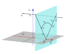
   Figure 1.

   By the triangle inequality,

   (2.51) $$\begin{split}&|\partial_{r_{n}}D^{\prime}h_{k}(p)-\partial_{r_{n}}D^{\prime}h_{k}(q)|\\ \leq&|\partial_{r_{n}}D^{\prime}h_{k}(p)-\partial_{r_{n}}D^{\prime}h_{k}(p^{\prime})|+|\partial_{r_{n}}D^{\prime}h_{k}(p^{\prime})-\partial_{r_{n}}D^{\prime}h_{k}(q^{\prime})|\\ &+|\partial_{r_{n}}D^{\prime}h_{k}(q^{\prime})-\partial_{r_{n}}D^{\prime}h_{k}(q)|.\end{split}$$

   Along $\gamma_{3}(\theta)$, we have (for notation convenience we write below $h_{k,ir_{n}}=\partial_{r_{n}}D^{\prime}_{i}h_{k}$)

   (2.52) $$|\partial_{r_{n}}D^{\prime}h_{k}(p)-\partial_{r_{n}}D^{\prime}h_{k}(p^{\prime})|=\left|\int_{\theta_{n}(p)}^{\theta_{n}(q)}\frac{\partial h_{k,ir_{n}}}{\partial\theta_{n}}d\theta_{n}\right|\leq Cr_{n}(p)^{\frac{1}{\beta}-1}\tau^{-k(\frac{1}{\beta}-1)}\omega(2\tau^{k}).$$

   Along $\gamma_{2}(t)$, we have

   (2.53) $$\begin{split}&|\partial_{r_{n}}D^{\prime}h_{k}(p^{\prime})-\partial_{r_{n}}D^{\prime}h_{k}(q^{\prime})|=\big{|}\int_{r_{n}(p)}^{r_{n}(q)}\frac{\partial h_{k,ir_{n}}}{\partial r_{n}}dt\big{|}\\ \leq&C\tau^{-k(\frac{1}{\beta}-1)}\omega(2\tau^{k})\int_{r_{n}(p)}^{r_{n}(q)}t^{\frac{1}{\beta}-2}dt\\ \leq&C\tau^{-k(\frac{1}{\beta}-1)}\omega(2\tau^{k})\big{|}r_{n}(q)^{\frac{1}{\beta}-1}-r_{n}(p)^{\frac{1}{\beta}-1}\big{|}\\ \leq&C\tau^{-k(\frac{1}{\beta}-1)}\omega(2\tau^{k})\big{|}r_{n}(q)-r_{n}(p)\big{|}^{\frac{1}{\beta}-1}\\ \leq&C\tau^{-k(\frac{1}{\beta}-1)}\omega(2\tau^{k})d^{\frac{1}{\beta}-1},\end{split}$$

   where we make use of the elementary inequality that for any $a,b>0$ and $\kappa\in(0,1)$,

   $$\big{|}a^{\kappa}-b^{\kappa}\big{|}\leq|a-b|^{\kappa}.$$

   Along $\gamma_{1}(t)$,

   (2.54) $$\begin{split}|\partial_{r_{n}}D^{\prime}h_{k}(q)-\partial_{r_{n}}D^{\prime}h_{k}(q^{\prime})|\leq&\big{|}(D^{\prime})^{2}\partial_{r_{n}}h_{k}\big{|}d\\ \leq&C\tau^{-k}\omega(2\tau^{k})d\\ \leq&C\tau^{-k(\frac{1}{\beta}-1)}d^{\frac{1}{\beta}-1}\omega(2\tau^{k}).\end{split}$$

2. $r_{p}\geq 2d$ and $\ell\leq k_{p}$. This case is relatively easier. By the triangle inequality, $r_{n}(t)=r_{n}(\gamma(t))\geq d$ for all $t\in[0,d]$. Along $\gamma(t)$,

   $$\big{|}\nabla_{g_{\beta}}(\partial_{r_{n}}D^{\prime}h_{k})\big{|}_{g_{\beta}}$$

   $$= \Big{(}\sum_{j=1}^{2n-2}\Big{(}\frac{\partial(\partial_{r_{n}}D^{\prime}h_{k})}{\partial s_{j}}\Big{)}^{2}+\Big{(}\frac{\partial(\partial_{r_{n}}D^{\prime}h_{k})}{\partial r_{n}}\Big{)}^{2}+\frac{1}{\beta^{2}r_{n}(t)^{2}}\Big{(}\frac{\partial(\partial_{r_{n}}D^{\prime}h_{k})}{\partial\theta_{n}}\Big{)}^{2}\Big{)}^{1/2}$$

   $$\leq C(n)\tau^{-k(\frac{1}{\beta}-1)}\omega(2\tau^{k})\Big{(}r_{n}(t)^{\frac{1}{\beta}-2}\Big{)}$$

   $$\leq C(n)\tau^{-k(\frac{1}{\beta}-1)}\omega(2\tau^{k})d^{\frac{1}{\beta}-2}.$$

   Integrating along the geodesic $\gamma$, we obtain the following desired estimate

   $$\big{|}(\partial_{r_{n}}D^{\prime}h_{k})(p)-(\partial_{r_{n}}D^{\prime}h_{k})(q)\big{|}\leq C(n)d^{\frac{1}{\beta}-1}\tau^{-k(\frac{1}{\beta}-1)}\omega(2\tau^{k}).$$

3. $r_{p}\geq 2d$ and $\ell>k_{p}$. In this case, we will replace $(s,z_{n})$ by $(s,w)$ for $w=(z_{n})^{\beta}$ in $B_{\beta}(p,\tau^{k})$, by taking a single-value branch, when $k_{p}<k\leq\ell$. The cone metric $g_{\beta}$ becomes the standard Euclidean metric in $(s,w)$ and

   $$\Delta_{g_{\beta}}(D^{\prime}h_{k})=\sum_{j=1}^{2n-2}\frac{\partial^{2}(D^{\prime}h_{k})}{\partial(s_{j})^{2}}+\sqrt{-1}\frac{\partial^{2}(D^{\prime}h_{k})}{\partial w\partial\overline{w}}=0,\text{ in }B_{\beta}(p,\tau^{k+1}).$$

   It then follows from the derivative estimates for Euclidean harmonic functions that

   $$\left\|\frac{\partial(D^{\prime}h_{k})}{\partial w}\right\|_{L^{\infty}(B_{\beta}(p,\tau^{k+2}))}\leq C\omega(\tau^{k}),$$

   $$\left\|\frac{\partial^{2}(D^{\prime}h_{k})}{\partial w\partial w}\right\|_{L^{\infty}(B_{\beta}(p,\tau^{k+2}))}+\left\|\frac{\partial^{2}(D^{\prime}h_{k})}{\partial w\partial\overline{w}}\right\|_{L^{\infty}(B_{\beta}(p,\tau^{k+2}))}\leq C\tau^{-k}\omega(\tau^{k}).$$

   Since

   $$2w\frac{\partial}{\partial w}=r_{n}\frac{\partial}{\partial r_{n}}-\frac{\sqrt{\smash[h]{-1}}}{\beta}\frac{\partial}{\partial\theta_{n}},\quad\frac{\partial}{\partial r_{n}}=\frac{w}{r_{n}}\frac{\partial}{\partial w}+\frac{\overline{w}}{r_{n}}\frac{\partial}{\partial\overline{w}},$$

   we have (denote $h_{k,i}=D^{\prime}_{i}h_{k}$)

   $$\frac{\partial}{\partial w}\Big{(}\frac{\partial h_{k,i}}{\partial r_{n}}\Big{)}= \frac{1}{r_{n}}\frac{\partial h_{k,i}}{\partial w}-\frac{w}{r_{n}^{2}}\frac{\overline{w}}{2r_{n}}\frac{\partial h_{k,i}}{\partial w}+\frac{w}{r_{n}}\frac{\partial^{2}h_{k,i}}{\partial w^{2}}$$

   $$-\frac{\overline{w}}{r_{n}^{2}}\frac{\overline{w}}{2r_{n}}\frac{\partial h_{k,i}}{\partial\overline{w}}+\frac{\overline{w}}{r_{n}}\frac{\partial^{2}h_{k,i}}{\partial w\partial\overline{w}}.$$

   Therefore

   (2.55) $$\begin{split}&\Big{|}\nabla\frac{\partial(D^{\prime}h_{k})}{\partial r_{n}}\Big{|}_{g_{\beta}}\\ \leq&C\Big{(}\frac{1}{r_{n}}\big{|}\frac{(D^{\prime}h_{k})}{\partial w}\big{|}+\big{|}\frac{\partial^{2}(D^{\prime}h_{k})}{\partial w\partial w}\big{|}+\frac{1}{r_{n}}\big{|}\frac{\partial(D^{\prime}h_{k})}{\partial w}\big{|}+\big{|}\frac{\partial^{2}(D^{\prime}h_{k})}{\partial w\partial\overline{w}}\big{|}+\tau^{-k}\omega(\tau^{k})\Big{)}\\ \leq&C\frac{1}{r_{n}}\omega(\tau^{k})+C\tau^{-k}\omega(\tau^{k}).\end{split}$$

   Let $\gamma$ be the minimal geodesic connecting $p$ and $q$ with respect to $g_{\beta}$. Then along $\gamma$, there exists $C>0$ such that

   $$r_{n}(\gamma(t))\geq Cr_{p}.$$

   After integrating along $\gamma$, it follows that

   $$\left|\frac{\partial(D^{\prime}h_{k})}{\partial r_{n}}(p)-\frac{\partial(D^{\prime}h_{k})}{\partial r_{n}}(q)\right|\leq C(n,\beta)d^{\frac{1}{\beta}-1}\tau^{-k(\frac{1}{\beta}-1)}\omega(\tau^{k}).$$

The estimate (2.48) is then proved by combining the above three cases. (2.49) can be proved by similar argument.

∎

Corollary 2.2.

There exists $C=C(n,\beta)>0$ such that

(2.56) $$\begin{split}&\big{|}\partial_{r_{n}}D^{\prime}u_{\ell}(p)-\partial_{r_{n}}D^{\prime}u_{\ell}(q)\big{|}+\big{|}\left((r_{n})^{-1}\partial_{\theta_{n}}D^{\prime}u_{\ell}\right)(p)-\left((r_{n})^{-1}\partial_{\theta_{n}}D^{\prime}u_{\ell}\right)(q)\big{|}\\ \leq&Cd^{\frac{1}{\beta}-1}\big{(}\|u\|_{L^{\infty}(B_{\beta}(0,1))}+\sum_{k=2}^{\ell}\tau^{-k(\frac{1}{\beta}-1)}\omega(\tau^{k})\big{)}.\end{split}$$

Proof.

The Corollary follows from (2.48) by similar argument in the proof to estimate $I_{2}$ in Proposition 2.3.

∎

The following proposition is the main result in this subsection.

Proposition 2.4.

Let $\beta\in(1/2,1)$. There exists $C=C(n,\beta)>0$ such that for all $p,q\in B_{\beta}(0,1/2)\backslash\mathcal{S}$,

(2.57) $$\begin{split}&\sum_{i=2n-1}^{2n}\sum_{j=1}^{2n-2}\left|D_{i}D_{j}u(p)-D_{i}D_{j}u(q)\right|\\ \leq&C\left(d^{\frac{1}{\beta}-1}\sup_{B_{\beta}(0,1)}|u|+\int_{0}^{d}\frac{\omega(r)}{r}dr+d^{\frac{1}{\beta}-1}\int_{d}^{1}\frac{\omega(r)}{r^{1/\beta}}dr\right),\end{split}$$

where $d=d_{\beta}(p,q).$

Proof.

The proposition is an immediate consequence of Lemma 2.11 and Corollary 2.2.

∎

2.7. Proof of Theorem 1.1

Theorem 1.1 immediately follows by combining Proposition 2.3 and Proposition 2.4.

2.8. The case of $\beta\in(0,1/2)$

If $\beta\in(0,1/2)$, Theorem 1.1 can be proved by parallel arguments for the case of $\beta\in(1/2,1)$ with slight modifications.

Proposition 2.5.

Suppose $\beta\in(0,1/2)$ and $f(x)$ is Dini continuous on $B_{\beta}(0,1)$ with respect to $g_{\beta}$ for some $\beta\in(0,1)$. Let

$$\omega(r)=\sup_{d_{\beta}(z,w)<r,~{}z,w\in B_{\beta}(0,1)}|f(z)-f(w)|.$$

If $u\in C^{2}(B_{\beta}(0,1)\setminus\mathcal{S})\cap L^{\infty}(B_{\beta}(0,1))$ is a solution of the conical Laplace equation (1.3), then there exists $C=C(n,\beta)>0$ such that

(2.58) $$\begin{split}&\sum_{i=2n-1}^{2n}\sum_{j=1}^{2n-2}|D_{i}D_{j}u(p)-D_{i}D_{j}u(q)|+\sum_{i,j=1}^{2n-2}|D_{i}D_{j}u(p)-D_{i}D_{j}u(q)|\\ \leq&C\left(d\sup_{B_{\beta}(0,1)}|u|+\int_{0}^{d}\frac{\omega(r)}{r}dr+d\int_{d}^{1}\frac{\omega(r)}{r^{2}}dr\right),\end{split}$$

where $d=d_{\beta}(p,q)$.

Proof.

Let us point out the major differences in the proof from that of Theorem 1.1. The estimate in Proposition 2.1 is pointwise:

$$\left|\frac{\partial u}{\partial z}(z)\right|\leq C\frac{\|u\|_{L^{\infty}(B_{\rho}(0))}}{\rho}+C\|F\|_{L^{\infty}(B_{\rho}(0))}|z|^{2\beta-1},\quad\forall z\in B_{\rho/2}(0)\backslash\{0\}.$$

With this estimate, the statements in Lemmas 2.12 and Lemma 2.13 are revised as follows.

1. Lemma 2.12:

   $$\left|\frac{\partial(D^{\prime}h_{k})}{\partial r_{n}}\right|(z)+\left|\frac{\partial(D^{\prime}h_{k})}{r_{n}\partial\theta_{n}}\right|(z)\leq Cr_{n}\tau^{-k}\omega(2\tau^{k}).$$

2. Lemma 2.13:

   $$\left|\frac{\partial^{2}(D^{\prime}h_{k})}{r_{n}^{2}\partial(\theta_{n})^{2}}\right|(z)+\left|\frac{\partial^{2}(D^{\prime}h_{k})}{r_{n}\partial r_{n}\partial\theta_{n}}\right|(z)+\left|\frac{\partial^{2}(D^{\prime}h_{k})}{\partial(r_{n})^{2}}\right|(z)\leq C\tau^{-k}\omega(2\tau^{k}).$$

∎

2.9. The case of $\beta=1/2$

In this case, $g_{\beta}$ is an orbifold metric. We can lift the equation on the double cover with $z_{n}=w^{2}$. Then the conical Laplace equation becomes the standard Laplace equation and one can directly apply the Schauder estimate on $\mathbb{R}^{2n}$. We obtain the same estimate as (2.58).

3. Parabolic Schauder estimates

The goal of this section is to derive the $\mathcal{P}_{\beta}^{2,\alpha}$-estimate of the parabolic equation

(3.1) $$\frac{\partial u}{\partial t}-\Delta_{g_{\beta}}u=f,\quad\text{in }\mathcal{Q}_{\beta},$$

where $f$ is a given Dini continuous function on $\overline{\mathcal{Q}_{\beta}}$ with respect to the conical parabolic distance.

3.1. Notations

We denote $\mathcal{Q}_{\beta}=B_{\beta}(0,1)\times(0,1]$ to be the space-time cylinder, and

$$\partial_{\mathcal{P}}\mathcal{Q}_{\beta}=\big{(}\overline{B_{\beta}(0,1)}\times\{0\}\big{)}\cup\big{(}\partial B_{\beta}(0,1)\times(0,1)\big{)}$$

to be the parabolic boundary of the cylinder $\mathcal{Q}_{\beta}$. Let

$$\mathcal{S}_{\mathcal{P}}=\{(p,t)~{}|~{}p\in\mathcal{S},~{}t\in\mathbb{R}\}$$

be the parabolic singular set. The conical parabolic distance of two points $Q_{1}=(z_{1},t_{1})$ and $Q_{2}=(z_{2},t_{2})$ in $\mathcal{Q}_{\beta}$ as

$$d_{\mathcal{P},\beta}(Q_{1},Q_{2})=\max\big{\{}d_{\beta}(z_{1},z_{2}),\sqrt{|t_{1}-t_{2}|}\big{\}}.$$

We denote

$$\omega(r)=\sup\{|f(Q_{1})-f(Q_{2})|:{{Q_{1},Q_{2}\in\overline{\mathcal{Q}_{\beta}},d_{P,\beta}(Q_{1},Q_{2})\leq r}}\}$$

to be the oscillation function of $f$ over the cylinder $\overline{\mathcal{Q}_{\beta}}$.

Definition 3.1.

We say a function $u$ is $\mathcal{P}^{2}$ in the cylinder $\mathcal{O}_{\beta}$, if for each time $t\in(0,1]$, $u(\cdot,t)\in C^{2}(B_{\beta}(0,1)\backslash\mathcal{S})$, and $\frac{\partial u}{\partial t}\in C^{0}(\mathcal{Q}_{\beta})$.

We define the $\mathcal{P}^{0,\alpha}_{\beta}$ norm of a function in $\mathcal{Q}_{\beta}$ similar to that in Definition 2.1, using the parabolic distance $d_{\mathcal{P},\beta}$. We define the $\mathcal{P}^{2,\alpha}_{\beta}$ norm in $\mathcal{Q}_{\beta}$ as

$$\begin{split}\|u\|_{\mathcal{P}^{2,\alpha}_{\beta}}=&\|u\|_{C^{0}(\mathcal{Q}_{\beta})}+\sum_{i=1}^{2n}\|D_{i}u\|_{C^{0}(\mathcal{Q}_{\beta})}+\|\partial_{t}u\|_{\mathcal{P}^{0,\alpha}_{\beta}(\mathcal{Q}_{\beta})}\\ &+\sum_{i=1}^{2n}\sum_{j=1}^{2n-2}\|D_{i}D_{j}u\|_{\mathcal{P}^{0,\alpha}_{\beta}(\mathcal{Q}_{\beta})}+\big{\|}|z_{n}|^{2-2\beta}\frac{\partial^{2}u}{\partial z_{n}\partial\overline{z}_{n}}\big{\|}_{\mathcal{P}^{0,\alpha}_{\beta}(\mathcal{Q}_{\beta})}\end{split}$$

Suppose $u\in\mathcal{P}^{2}(\mathcal{Q}_{\beta}\setminus\mathcal{S}_{\mathcal{P}})\cap C^{0}(\overline{\mathcal{Q}_{\beta}})$ solves the Dirichlet problem for the conical heat equation

(3.2) $$\left\{\begin{aligned} \frac{\partial u}{\partial t}-\Delta_{g_{\beta}}u=0,\quad\text{in }\mathcal{Q}_{\beta}\\ u(z,t)=\varphi(z,t),\quad\text{on }\partial_{\mathcal{P}}\mathcal{Q}_{\beta},\end{aligned}\right.$$

for some given continuous function $\varphi\in C^{0}(\partial_{\mathcal{P}}\mathcal{Q}_{\beta})$. Without loss of generality, we assume $\varphi$ can be continuously extended to $\overline{\mathcal{Q}_{\beta}}$.

Applying the same barrier function as in Lemma 2.1, we have the following maximum principle for the conical heat equation.

Lemma 3.1.

Suppose $u\in\mathcal{P}^{2}(\mathcal{Q}_{\beta}\backslash\mathcal{S}_{\mathcal{P}})\cap C^{0}(\overline{\mathcal{Q}_{\beta}})$ solves the equation (3.2), then

$$\inf_{\overline{\mathcal{Q}_{\beta}}}\varphi\leq\inf_{\mathcal{Q}_{\beta}}u\leq\sup_{\mathcal{Q}_{\beta}}u\leq\sup_{\overline{\mathcal{Q}_{\beta}}}\varphi.$$

In particular, the conical heat equation (3.2) admits a unique solution.

Corollary 3.1.

If the Dirichlet boundary value problem (3.2) is solvable in $\mathcal{P}^{2}(\mathcal{Q}_{\beta}\backslash\mathcal{S}_{\mathcal{P}})\cap C^{0}(\overline{\mathcal{Q}_{\beta}})$, the solution must be unique.

3.2. Conical heat equations

In this subsection, we will obtain a parabolic gradient estimate of Li-Yau for conical heat equation. The following proposition is the standard Li-Yau gradient estimate for positive solution to the heat equation ([16], see also Theorem 4.2 in [26]).

Proposition 3.1.

Let $(M,g)$ be a complete manifold with $\mathrm{Ric}(g)\geq 0$, and $B(p,R)$ be the geodesic ball with center $p\in M$ and radius $R>0$. Let $u$ be a positive solution to the heat equation $\partial_{t}u-\Delta_{g}u=0$ on $B(p,R)$, then there exists $C=C(n)>0$ such that for all $t>0$,

$$\sup_{B(p,R/2)}\Big{(}\frac{|\nabla u|^{2}}{u^{2}}-\frac{2u_{t}}{u}\Big{)}\leq\frac{C}{R^{2}}+\frac{2n}{t},$$

where $u_{t}=\frac{\partial u}{\partial t}$.

The following corollary is a straightforward consequence of Proposition 3.1.

Corollary 3.2.

With the same assumptions in Proposition 3.1, there exists $C=C(n)>0$ such that for all $t\in(0,R^{2})$

$$\sup_{B(p,R/2)}|\nabla u|^{2}(t)\leq C\Big{(}\frac{1}{R^{2}}+\frac{1}{t}\Big{)}\left(\operatorname{osc}_{B(p,R)\times[0,R^{2}]}u\right)^{2}$$

and

$$\sup_{B(p,R/2)}\big{|}\Delta_{g}u\big{|}(t)=\sup_{B(p,R/2)}\big{|}\frac{\partial u}{\partial t}\big{|}\leq C\Big{(}\frac{1}{R^{2}}+\frac{1}{t}\Big{)}\left(\operatorname{osc}_{B(p,R)\times[0,R^{2}]}u\right).$$

Proof.

Replacing the positive solution $u$ by $u-\inf u$ if necessary, we may assume that $u\leq\operatorname{osc}u$. We let $A=\sup_{B(p,R)\times[0,R^{2}]}u$ and $v=A-u$. Clearly $v$ also satisfies the heat equation and by Li-Yau gradient estimates we have on $B(p,R/2)$,

(3.3) $$\frac{|\nabla u|^{2}}{v}\leq 2v_{t}+C\Big{(}\frac{1}{R^{2}}+\frac{1}{t}\Big{)}v=-2u_{t}+C\Big{(}\frac{1}{R^{2}}+\frac{1}{t}\Big{)}v,$$

and by Proposition 3.1 we also have

(3.4) $$\frac{|\nabla u|^{2}}{u}\leq 2u_{t}+C\Big{(}\frac{1}{R^{2}}+\frac{1}{t}\Big{)}u.$$

Adding (3.3) and (3.4), we have

$$\Big{(}\frac{1}{u}+\frac{1}{v}\Big{)}|\nabla u|^{2}\leq C\Big{(}\frac{1}{R^{2}}+\frac{1}{t}\Big{)}\big{(}u+v\big{)},$$

from which it follows that on $B(p,R/2)$

$$|\nabla u|^{2}\leq C\Big{(}\frac{1}{R^{2}}+\frac{1}{t}\Big{)}u(A-u)\leq C\Big{(}\frac{1}{R^{2}}+\frac{1}{t}\Big{)}\left(\operatorname{osc}_{B(p,R)\times[0,R^{2}]}u\right)^{2}.$$

The estimate for $\Delta u$ follows easily from the fact that $\frac{\partial u}{\partial t}=\Delta u$.

∎

Given Corollary 3.2, we are ready to show the existence of solution to the equation (3.2).

Proposition 3.2.

Given any $\varphi\in C^{0}(\overline{\mathcal{Q}_{\beta}})$, there exists a unique $u\in\mathcal{P}^{2}(\mathcal{Q}_{\beta}\setminus\mathcal{S}_{\mathcal{P}})\times C^{0}(\overline{\mathcal{Q}_{\beta}})$ solving equation (3.2).

Proof.

The strategy is to solve the Dirichlet boundary problem for the smooth metrics $g_{\epsilon}$ approximating the conical metric $g_{\beta}$ and the limiting solution will solve (3.2).

Let $u_{\epsilon}\in\mathcal{P}^{2}(\mathcal{Q}_{\beta})\cap C^{0}(\overline{\mathcal{Q}_{\beta}})$ solve the Dirichlet boundary problem

(3.5) $$\left\{\begin{aligned} \frac{\partial u_{\epsilon}}{\partial t}=\Delta_{g_{\epsilon}}u_{\epsilon},\quad\text{in }\mathcal{Q}_{\beta}\\ u_{\epsilon}=\varphi,\quad\text{on }\partial_{\mathcal{P}}\mathcal{Q}_{\beta},\end{aligned}\right.$$

where $g_{\epsilon}$ is a smooth Riemannian metric defined in (2.6) to approximate $g_{\beta}$ for $\epsilon\in(0,1)$. We immediately have following estimate by the maximum principle.

$$\|u_{\epsilon}\|_{L^{\infty}(\mathcal{Q}_{\beta})}\leq\|\varphi\|_{L^{\infty}(\overline{\mathcal{Q}_{\beta}})}.$$

Let $K\subset\subset K^{\prime}\subset\subset B_{\beta}(0,1)$ be arbitrarily compact subsets in $B_{\beta}(0,1)$. Applying Corollary 3.2, we have

(3.6) $$\sup_{K^{\prime}}|\nabla u_{\epsilon}|^{2}_{g_{\epsilon}}(\cdot,t)\leq C(n,K^{\prime},\|\varphi\|_{\infty})\big{(}1+t^{-1}\big{)},$$

(3.7) $$\sup_{K^{\prime}}\big{|}\frac{\partial u_{\epsilon}}{\partial t}\big{|}\leq C(n,K^{\prime},\|\varphi\|_{\infty})\big{(}1+t^{-1}\big{)}$$

Similarly we have

(3.8) $$\sup_{K}|\nabla(D^{\prime}u_{\epsilon})|^{2}_{g_{\epsilon}}\leq C(n,K,K^{\prime},\|\varphi\|_{\infty})\big{(}1+t^{-2}\big{)},$$

and

(3.9) $$\sup_{K}|\nabla\left((D^{\prime})^{2}u_{\epsilon}\right)|^{2}_{g_{\epsilon}}\leq C(n,K,K^{\prime},\|\varphi\|_{\infty})\big{(}1+t^{-3}\big{)}.$$

It follows from the standard elliptic estimates that the functions $u_{\epsilon}$ have uniform $\mathcal{P}^{2,\alpha}$ estimates on $K\backslash T_{\delta}(\mathcal{S})\times[\delta,1]$, for a fixed $\delta>0$. So $u_{\epsilon}$ converges uniformly in $\mathcal{P}^{2,\alpha}(K\backslash T_{\delta}(\mathcal{S})\times[\delta,1])$-topology to a function $u\in\mathcal{P}^{2,\alpha}(K\backslash T_{\delta}(\mathcal{S})\times[\delta,1])$. Since $K$ is arbitrary, by taking a diagonal sequence, we may assume $u_{\epsilon}$ converges to $u$ uniformly on any compact subset of $B_{\beta}(0,1)\backslash\mathcal{S}\times(0,1]$. Clearly $u$ satisfies the equation $\partial_{t}u=\Delta_{g_{\beta}}u$ on $B_{\beta}\backslash\mathcal{S}\times(0,1]$ and the estimates (3.6), (3.7) and (3.8). In particular (3.6) implies that $u$ can be continuously extended over $\mathcal{S}$, so $u\in C^{0}(B_{\beta}\times(0,1])$.

It remains to show $u$ is continuous up to boundary and it coincides with $\varphi$ on $\partial_{\mathcal{P}}\mathcal{Q}_{\beta}$. We will show that for any $(q,t_{0})\in\partial_{\mathcal{P}}\mathcal{Q}_{\beta}$,

$$\lim_{\mathcal{Q}_{\beta}\ni(z,t)\to(q,t_{0})}u(z,t)=\varphi(q,t_{0}).$$

Case 1: $t_{0}=0$ and $q\in\overline{B_{\beta}(0,1)}$. We will construct the barrier function

$$\phi_{q,1}(z,t)=e^{-d_{\mathbb{C}^{n}}(z,q)^{2}-\lambda t}-1,$$

where $d_{\mathbb{C}^{n}}$ is the Euclidean distance and $\lambda>0$ is a constant to be determined. Direct calculations show that

$$\Delta_{g_{\epsilon}}\phi_{q,1}= \big{(}-\Delta_{\epsilon}d_{\mathbb{C}^{n}}^{2}+|\nabla d^{2}_{\mathbb{C}^{n}}|^{2}_{g_{\epsilon}}\big{)}e^{-d_{\mathbb{C}^{n}}(z,q)^{2}-\lambda t}$$

$$= \big{(}-(n-1)-(|z_{n}|^{2}+\epsilon)^{1-\beta}+|\nabla d_{\mathbb{C}^{n}}^{2}|^{2}_{g_{\epsilon}}\big{)}e^{-d_{\mathbb{C}^{n}}(z,q)^{2}-\lambda t}$$

$$\geq -(n+1)e^{-d_{\mathbb{C}^{n}}(z,q)^{2}-\lambda t}$$

$$\geq -\lambda e^{-d_{\mathbb{C}^{n}}(z,q)^{2}-\lambda t}=\frac{\partial\phi_{q,1}}{\partial t},$$

if we choose $\lambda\geq n+1$. $\phi_{q,1}$ is a continuous function on $\overline{\mathcal{Q}_{\beta}}$ with $\phi_{q,1}(q,t_{0})=0$ and $\phi_{q,1}(z,t)<0$ for any other $(z,t)\in\overline{\mathcal{Q}_{\beta}}$.

For any fixed $\delta>0$, by the continuity of $\varphi$ it follows that there exists a small space-time neighborhood $V$ of $(q,t_{0})$ such that $\varphi(q,t_{0})-\delta\leq\varphi(z,t)$ for all $(z,t)\in V$. Moreover, on $\overline{\mathcal{Q}_{\beta}}\backslash V$ the function $\phi_{q}$ is bounded above by a negative constant, so by taking sufficiently large $A>0$, the function $\varphi_{q}^{-}$ defined by

$$\varphi_{q}^{-}(z,t):=\varphi(q,t_{0})-\delta+A\phi_{q,1}(z,t)\leq\varphi(z,t),$$

is a sub-solution of the heat equation, i.e. $\frac{\partial\varphi_{q}^{-}}{\partial t}\leq\Delta_{\epsilon}\varphi_{q}^{-}$. Then $\varphi_{q}^{-}(z,t)\leq u_{\epsilon}(z,t)$ for all $(z,t)\in\mathcal{Q}_{\beta}$ by the maximum priniciple. Letting $\epsilon\to 0$, we also have $\varphi_{q}^{-}(z,t)\leq u(z,t)$ and so

$$\varphi(q,t_{0})-\delta=\lim_{(z,t)\to(q,t_{0})}\varphi^{-}_{q}(z,t)\leq\liminf_{(z,t)\to(q,t_{0})}u(z,t).$$

Letting $\delta\to 0$, $\varphi(q,t_{0})\leq\liminf_{(z,t)\to(q,t_{0})}u(z,t)$.

By similar argument we can show that $\varphi(q,t_{0})\geq\limsup_{(z,t)\to(q,t_{0})}u(z,t)$ by considering the super-solution $\varphi_{q}^{+}(z,t)=\varphi(q,t_{0})+\delta-A\phi_{q}(z,t)$ for appropriate $A>0$. Therefore,

$$\lim_{(z,t)\to(q,t_{0})}u(z,t)=\varphi(q,t_{0}).$$

Case 2: $t_{0}>0$ and $q\in\partial B_{\beta}(0,1)$ with $z_{n}(q)=0$. Let $q^{\prime}=-q\in\mathbb{C}^{n}$ be the opposite point of $q$ with respect to $0\in\mathbb{C}^{n}$. We define the barrier function

$$\phi_{q,2}(z,t)=d_{\mathbb{C}^{n}}(z,q^{\prime})^{2}-4-\delta(t-t_{0})^{2}$$

for a small $\delta>0$ to be determined. Since $q$ is the unique furthest point in $B_{\beta}(0,1)$ to $q^{\prime}$ under Euclidean distance, hence $\phi_{q,2}(q,t_{0})=0$ and $\phi_{q,2}(z,t)<0$ for all other $(z,t)\in\overline{\mathcal{Q}_{\beta}}$. Straightforward calculations show that

$$\frac{\partial\phi_{q,2}}{\partial t}=-2\delta(t-t_{0}),$$

and

$$\Delta_{\epsilon}\phi_{q,2}=(n-1)+\beta^{-2}(|z_{n}|^{2}+\epsilon)^{1-\beta}\geq n-1.$$

Then $\partial_{t}\phi_{q,2}\leq\Delta_{\epsilon}\phi_{q,2}$ for $\delta\leq(n-1)/2$. By the same argument as in Case 1, we see that $u$ is also continuous at $(q,t_{0})\in\partial_{\mathcal{P}}\mathcal{\mathcal{Q}_{\beta}}$ and $\lim_{(z,t)\to(q,t_{0})}u(z,t)=\varphi(q,t_{0}).$

Case 3: $t_{0}>0$ and $q\in\partial B_{\beta}(0,1)$ with $z_{n}(q)\neq 0$. We are in the same situation as the case 2 in the proof of Proposition 2.2, and we use the same notations as in Proposition 2.2. We construct the following barrier function

$$\phi_{q,3}(z,t)=A\Big{(}d_{\beta}(z)^{2}-1\Big{)}+\Big{(}G(z)-\frac{1}{r_{q}^{2n-2}}\Big{)}-\delta^{\prime}(t-t_{0})^{2}.$$

The remaining argument is the same as in Case 1 and Case 2.

Combining the results in the above three cases, we have completed the proof of the proposition.

∎

Furthermore, we also obtaine the conical gradient and Laplace estimates for $u$.

Corollary 3.3.

Let $u\in\mathcal{P}^{2}(B_{\beta}(0,R)\times(0,R^{2}])\cap L^{\infty}(\overline{B_{\beta}(0,R)}\times[0,R^{2}])$ solve the heat equation $\partial_{t}u=\Delta_{\beta}u$ in $B_{\beta}(0,R)\backslash\mathcal{S}\times(0,R^{2}]$. There exists a constant $C=C(n)$ such that

$$\sup_{B_{\beta}(0,R/2)\backslash\mathcal{S}}|\nabla u|^{2}_{g_{\beta}}\leq C\Big{(}\frac{1}{R^{2}}+\frac{1}{t}\Big{)}\|u\|_{L^{\infty}(B_{\beta}(0,R)\times[0,R^{2}])}^{2},$$

$$\sup_{B_{\beta}(0,R/2)\backslash\mathcal{S}}\big{|}\Delta_{\beta}u\big{|}=\sup_{B_{\beta}(0,R/2)\backslash\mathcal{S}}\big{|}\frac{\partial u}{\partial t}\big{|}\leq C\Big{(}\frac{1}{R^{2}}+\frac{1}{t}\Big{)}\|u\|_{L^{\infty}(B_{\beta}(0,R)\times[0,R^{2}])}.$$

Moreover, the function $\frac{\partial u}{\partial t}$ can be continuously extended to $B_{\beta}(0,1)$.

3.3. Proof of Theorem 1.2

We can now prove Theorem 1.2 by the same argument in the proof of Theorem 1.1, replacing the $g_{\beta}$-harmonic functions by solutions of $g_{\beta}$-heat equation, since we have obtained existence and gradient estimate for solutions of conical heat equation (3.2) from Proposition 3.2 and Corollary 3.3.

Acknowledgements: Both authors thank Duong H. Phong and Qing Han for many insightful discussions.

References

- [1] Brendle, S. Ricci flat Kähler metrics with edge singularities, Int. Math. Res. Not. IMRN 2013, no. 24, 5727–5766
- [2] Caffarelli, L.A. Interior a priori estimates for solutions of fully nonlinear equations, Ann. of Math. (2) 130 (1989), 189–213
- [3] Caffarelli, L.A. Interior W2,p estimates for solutions of Monge-Ampère equations, Ann. Math., 131(1990), 135–150
- [4] Chen, X.X., Donaldson, S.K. and Sun, S. Kähler-Einstein metrics on Fano manifolds, I: approximation of metrics with cone singularities, J. Amer. Math. Soc. 28 (2015), no. 1, 183–197.
- [5] Chen, X.X., Donaldson, S.K. and Sun, S. Kähler-Einstein metrics on Fano manifolds, II: limits with cone angle less than , J. Amer. Math. Soc. 28 (2015), no. 1, 199–234
- [6] Chen, X.X., Donaldson, S.K. and Sun, S. Kähler-Einstein metrics on Fano manifolds, III: limits as cone angle approaches and completion of the main proof, J. Amer. Math. Soc. 28 (2015), no. 1, 235–278
- [7] Chen, X.X. and Wang, Y. Bessel functions, heat kernel and the conical Kähler-Ricci flow. J. Funct. Anal. 269 (2015), no. 2, 551–632
- [8] Cheng and Yau, Differential equations on Riemannian manifolds and their geometric applications. Comm. Pure Appl. Math. 28 (1975), no. 3, 333–354
- [9] Donaldson, S. K. Kähler metrics with cone singularities along a divisor. Essays in mathematics and its applications, 49–79, Springer, Heidelberg, 2012
- [10] Edwards, G. A scalar curvature bound along the conical Kähler-Ricci flow, preprint arXiv:1505.02083.
- [11] Han, Q., and Lin, F. Elliptic partial differential equations (Vol. 2), American Mathematical Soc.
- [12] Hormander, L. An introduction to complex analysis in several variables. Second revised edition. North-Holland Mathematical Library, Vol. 7. North-Holland Publishing Co., Amsterdam-London; American Elsevier Publishing Co., Inc., New York, 1973. x+213 pp.
- [13] Jeffres, T., Mazzeo, R. and Rubinstein, Y. Kähler-Einstein metrics with edge singularities with appendix by Rubinstein Y. and Li, C., Ann. of Math. (2) 183 (2016), no. 1, 95–176
- [14] Jin, X., Liu, J. and Zhang, X. Twisted and conical Kähler-Ricci solitons on Fano manifolds, J. Funct. Anal. 271 (2016), no. 9, 2396–2421
- [15] Kolodziej, S. The complex Monge-Ampère equation, Acta Math. 180 (1998),69–117
- [16] Li, P. and Yau, S.-T. On the parabolic kernel of the Schrödinger operator. Acta Math. 156 (1986), no. 3–4, 153–201
- [17] Luo, F. and Tian, G. Liouville equation and spherical convex polytopes, Proc. Amer. Math. Soc. 116 (1992), 1119–1129
- [18] Mazzeo, R. Kähler-Einstein metrics singular along a smooth divisor, Journées Eq́uations aux dérivées partielles (1999), 1–10
- [19] Phong, D. H., Song, J., Sturm, J. and Wang, X. The Ricci flow on the sphere with marked points, preprint arXiv:1407.1118.
- [20] Rubinstein, Y. Smooth and singular Kähler-Einstein metrics, Geometric and spectral analysis, 45–138, Contemp. Math., 630, Amer. Math. Soc., Providence, RI, 2014
- [21] Mazzeo, R, Rubinstein, Y. and Sesum, N. Ricci flow on surfaces with conic singularities. Anal. PDE 8 (2015), no. 4, 839–882
- [22] Safonov, M.V. The classical solution of the elliptic Bellman equation , Dokl. Akad. Nauk SSSR 278(1984), 810–813; English translation in Soviet Math Doklady 30(1984), 482–485
- [23] Safonov, M.V. Classical solution of second-order nonlinear elliptic equations, Izv. Akad. Nauk SSSR Ser. Mat. 52(1988), 1272–1287; English translation in Math. USSR-Izv. 33(1989), 597–612
- [24] Simon, L. Schauder estimates by scaling, Calc. Var. PDE, 5(1997), 391–407
- [25] Song, J. and Wang, X. The greatest Ricci lower bound, conical Einstein metrics and Chern number inequality. Geom. Topol. 20 (2016), no. 1, 49–102
- [26] Schoen, R. and Yau, S.-T. Lectures on differential geometry. Conference Proceedings and Lecture Notes in Geometry and Topology, I. International Press, Cambridge, MA, 1994. v+235 pp.
- [27] Tian, G. On Kähler-Einstein metrics on certain Kähler manifolds with . Invent. Math. 89 (1987), no. 2, 225–246
- [28] Tian, G. Kähler-Einstein metrics on algebraic manifolds. Transcendental methods in algebraic geometry, 143б85, Lecture Notes in Math., 1646, Springer, Berlin, 1996
- [29] Tian, G. K-stability and Kähler-Einstein metrics, Comm. Pure Appl. Math. 68 (2015), no. 7, 1085–1156
- [30] Troyanov, M. Prescribing curvature on compact surfaces with conic singularities, Trans. Amer. Math. Soc. 324 (1991), 793–821
- [31] Wang, X.-J. Schauder estimates for elliptic and parabolic equations. Chinese Ann. Math. Ser. B 27 (2006), no. 6, 637–642
- [32] Yau, S.-T. On the Ricci curvature of a compact Kähler manifold and the complex Monge-Ampère equation, I, Comm. Pure Appl. Math. 31 (1978), no. 3, 339–411
- [33] Yin, H. Analysis aspects of Ricci flow on conical surfaces, preprint arXiv:1605.08836
- [34] Yin, H. and Zheng, K. Expansion formula for complex Monge-Ampère equation along cone singularities, preprint arXiv:1609.03111