Learning molecular energies using localized graph kernels

Abstract

Recent machine learning methods make it possible to model potential energy of atomic configurations with chemical-level accuracy (as calculated from ab-initio calculations) and at speeds suitable for molecular dynamics simulation. Best performance is achieved when the known physical constraints are encoded in the machine learning models. For example, the atomic energy is invariant under global translations and rotations; it is also invariant to permutations of same-species atoms. Although simple to state, these symmetries are complicated to encode into machine learning algorithms. In this paper, we present a machine learning approach based on graph theory that naturally incorporates translation, rotation, and permutation symmetries. Specifically, we use a random walk graph kernel to measure the similarity of two adjacency matrices, each of which represents a local atomic environment. This Graph Approximated Energy (GRAPE) approach is flexible and admits many possible extensions. We benchmark a simple version of GRAPE by predicting atomization energies on a standard dataset of organic molecules.

I Introduction

There is a large and growing interest in applying machine learning methods to infer molecular properties and potential energies Ho and Rabitz (1996); Bettens and Collins (1999); Braams and Bowman (2009); Hansen et al. (2013); Rupp et al. (2015); Bartók and Csányi (2015) based upon data generated from ab initio quantum calculations. Steady improvement in the accuracy, transferability, and computational efficiency of the machine learned models has been achieved. A crucial enabler, and ongoing challenge, is incorporating prior physical knowledge into the methodology. In particular, we know that potential energies should be invariant with respect to translations and rotations of atomic positions, and also with respect to permutations of identical atoms. The search for new techniques that naturally encode physical invariances is of continuing interest.

A common modeling approach is to decompose the energy of an atomic configuration as a sum of local contributions, and to represent each local atomic environment in terms of descriptors (i.e. features) that are inherently rotation and permutation invariant Behler (2011); Bartók et al. (2013). Such descriptors may be employed in, e.g., linear regression Thompson et al. (2015) or neural network models Behler and Parrinello (2007); Handley and Behler (2014); Behler (2014, 2015); Schütt et al. (2017). Recently, sophisticated descriptors have been proposed based on an expansion of invariant polynomials Shapeev (2015) and, inspired by convolutional neural networks, on a cascade of multiscale wavelet transformations Hirn et al. (2015, 2016).

Kernel learning is an alternative approach that can avoid direct use of descriptors Hofmann et al. (2008); Scholkopf and Smola (2001). Instead, one specifies a kernel that measures similarity between two inputs and, ideally, directly satisfies known invariances. An advantage of kernel methods is that the accuracy can systematically improve by adding new configurations to the dataset. A disadvantage is that the computational cost to build a kernel regression model typically scales cubically with dataset size. Kernel methods that model potential energies include Gaussian Approximation Potentials (GAP) Bartók et al. (2010), Smooth Overlap of Atomic Potentials (SOAP) Bartók et al. (2013); Bartók and Csányi (2015), methods based upon eigenvalues of the Coulomb matrix Rupp et al. (2012), Bag-of-Bonds Hansen et al. (2015), and others Hansen et al. (2013); Schütt et al. (2014); Li et al. (2015); Ferré et al. (2015). However, encoding the physical invariances may impose challenges. For example, to achieve rotational invariance in GAP and SOAP, one requires explicit integration over the relative rotation of two configurations. To achieve permutation invariance in methods based upon the Coulomb matrix, one commonly restricts attention to sorted descriptors (e.g. matrix eigenvalues or Bag-of-Bonds), thus introducing singularities in the regression model, and potentially also sacrificing discriminative power.

Here, we present the Graph Approximated Energy (GRAPE) framework. GRAPE is based on two central ideas: we represent local atomic environments as weighted graphs based upon pairwise distances, for which rotation invariance is inherent, and we compare local atomic environments by leveraging well known graph kernel methods invariant with respect to node permutation. There is much flexibility in implementing these ideas. In this paper, we define the weighted adjacency matrix elements (i.e. the edge weights) through an analogy with SOAP Bartók et al. (2013), and we use generalized random walk graph kernels Gärtner et al. (2002, 2003); Vishwanathan et al. (2010) to define similarity between graphs. Graph kernels have commonly been employed to compare molecules and predict their properties Drews (2000); Smola and Kondor (2003); Borgwardt and Kriegel (2005); Ralaivola et al. (2005); Sharan and Ideker (2006); Schietgat et al. (2008); Smalter et al. (2009); Vishwanathan et al. (2010); Gaüzere et al. (2012), but it appears that prior applications to energy regression are limited Sun (2014). We demonstrate with benchmarks that GRAPE shows promise for energy regression tasks.

The rest of the paper is organized as follows. Section II reviews necessary background techniques: kernel ridge regression of energies, the SOAP kernel, and random walk graph kernels. We merge these tools to obtain our GRAPE kernel, presented in Sec. III. Finally, we demonstrate the performance of GRAPE on a standard molecular database in Sec. IV and summarize our results in Sec. V.

II Review of relevant methods

II.1 Kernel modeling of potential energy

Here we review the machine learning technique of kernel ridge regression and its application to modeling potential energy landscapes. We assume a dataset $(x_{i},y_{i})_{i=1\dots N}$, where $x_{i}$ represents an atomic configuration and $y_{i}=E(x_{i})$ its corresponding energy. The goal is to build a statistical approximation $\hat{E}$ that accurately estimates the energy of new configurations.

A common approach begins with descriptors (also called features or order parameters) $(h_{m})_{m=1\dots M}$, designed to capture various aspects of a configuration $x$. Often $h_{m}(x)$ describes the geometry of a local atomic environment. Many descriptors suitable for modeling potential energy have been developed Bartók et al. (2013). The descriptors can be used, for example, with simple linear regression Thompson et al. (2015),

$$\hat{E}(x)=\sum_{m=1}^{M}\beta_{m}h_{m}(x),$$ (1)

with learned regression coefficients $\beta_{m}$, or as inputs to a more complicated model such as a neural network Behler (2015).

Kernel methods are an alternative machine learning approach, and avoid direct use of descriptors. Instead, the starting point is a kernel $K(x,x^{\prime})$ that measures the similarity between configurations $x$ and $x^{\prime}$. We use kernel ridge regression, for which the approximated energy reads

$$\left\{\begin{array}[]{rl}\displaystyle\hat{E}(x)&\displaystyle=\sum_{i=1}^{N}\hat{\alpha}_{i}K(x_{i},x),\\ \displaystyle\hat{\alpha}&\displaystyle=(K+\lambda I)^{-1}y,\end{array}\right.$$ (2)

where $I\in\mathbb{R}^{N\times N}$ is the identity matrix, $K\in\mathbb{R}^{N\times N}$ denotes a matrix with elements $K(x_{i},x_{j})$, and $y=(y_{1},y_{2},\dots,y_{N})$ are the energies in the dataset. The parameter $\lambda>0$ serves to regularize the model, and prevents overfitting by penalizing high frequencies Hofmann et al. (2008).

Equations (2) can be readily derived from the linear model, (1), using least squares error minimization with a ridge penalty; see Appendix A for details. The kernel becomes $K(x,x^{\prime})=\sum_{m=1}^{M}h_{m}(x)h_{m}(x^{\prime})$, and thus satisfies the criteria of symmetry and positive semi-definiteness. Conversely, any function $K$ that is symmetric and positive semi-definite can be decomposed as above, where $M$ may be infinite Mercer (1909). Thus, $(h_{m})_{m=1\dots M}$ and $K$ are formally interchangeable. An advantage of specifying the kernel directly is that the corresponding, potentially infinite set of descriptors may remain fully implicit.

In the context of modeling potential energies and forces, physical locality is often a good approximation Bartók and Csányi (2015). We assume that the energy of an atomic configuration $x_{i}$ with $n_{i}$ atoms can be decomposed as a sum of local contributions,

$$E(x)=\sum_{\ell=1}^{n_{i}}\varepsilon(\tilde{x}_{i,\ell}),$$ (3)

where $\tilde{x}_{i,\ell}$ denotes a local view of environment $x_{i}$ centered on atom $\ell$. The index $\ell$ iterates through all $n_{i}$ atoms of the atomic configuration $x_{i}$, and we denote by $Q=\sum_{i=1}^{N}n_{i}$ the total number of local environments in the database. If long-range interactions exist, e.g. induced by electrostatics, they should be treated separately from (3).

The key idea is that statistical regression should begin with the local energy $\varepsilon$, which we formally decompose as in (1). Then, after a series of straightforward steps (Appendix B), we find Bartók and Csányi (2015)

$$K(x_{i},x_{i^{\prime}})=\sum_{\ell=1}^{n_{i}}\sum_{\ell^{\prime}=1}^{n_{i^{\prime}}}\tilde{K}(\tilde{x}_{i,\ell},\tilde{x}^{\prime}_{i^{\prime},\ell^{\prime}}),$$ (4)

and the localized kernel regression finally reads for a configuration $x$:

$$\left\{\begin{array}[]{rl}\displaystyle\hat{E}(x)&=\displaystyle\sum_{i=1}^{N}\hat{\alpha}_{i}\sum_{\ell=1}^{n_{i}}\sum_{\ell^{\prime}=1}^{n}\tilde{K}(\tilde{x}_{i,\ell},\tilde{x}_{\ell^{\prime}}),\\ \displaystyle\hat{\alpha}&=\displaystyle(L\tilde{K}L^{T}+\lambda I)^{-1}y,\end{array}\right.$$ (5)

where the entries of the matrix $\tilde{K}\in\mathbb{R}^{Q\times Q}$ are $\tilde{K}(x_{i,\ell},x_{i^{\prime},\ell^{\prime}})$ (i.e. the similarity between local environments $\ell$ and $\ell^{\prime}$ in configurations $i$ and $i^{\prime}$), and $L\in\mathbb{R}^{N\times Q}$ is such that $L_{i,\ell}=1$ if the local environment $\ell$ belongs to configuration $i$ and $0$ otherwise.

The important conclusion is that the kernel $\tilde{K}$ for local configurations confers a kernel $K$ for total configurations. This is a mathematical consequence of the energy decomposition, which encodes locality into our statistical model of global energies. Note that the energies $\varepsilon$ of the local atomic configurations $\tilde{x}_{\ell}$ need not be explicitly learned. The relatively small size of $\tilde{x}_{\ell}$ improves computational efficiency, and generally enhances transferability of the model.

To summarize, Eqs. (4) and (5) provide the recipe for kernel ridge regression of energy. The rest of the paper discusses approaches to designing the local kernel $\tilde{K}$.

II.2 SOAP kernel

Here we review the powerful SOAP method Bartók et al. (2013); Bartók and Csányi (2015) for regression of potential energy landscapes. The structure of the SOAP kernel will inspire our design of GRAPE, which we present in Sec. III.

We begin by representing the local configuration $\tilde{x}_{\ell}$ with $\tilde{n}_{\ell}$ neighbors as a smooth atomic density centered on atom $\ell$,

$$\rho_{\tilde{x}_{\ell}}(\mathbf{r})=\sum_{i=1}^{\tilde{n}_{\ell}}\omega(z_{i})f_{\mathrm{c}}(|\mathbf{r}_{i\ell}|)\varphi_{\sigma}(|\mathbf{r}-\mathbf{r}_{i\ell}|).$$ (6)

Here $\mathbf{r}_{i\ell}=\mathbf{r}_{i}-\mathbf{r}_{\ell}$, with $\mathbf{r}_{i}$ the position of the $i^{\mathrm{th}}$ atom in $\tilde{x}_{\ell}$ and $z_{i}$ its atomic number with associated weight $\omega(z_{i})$. There is flexibility is choosing the coefficient $\omega(z_{i})$, provided that it is an injective function of the atomic number $z_{i}$ for atom $i$. We also define a Gaussian function to smooth the atomic densities,

$$\varphi_{\sigma}(r)=\exp(-r^{2}/2\sigma^{2}),$$ (7)

and a cut-off function,

$$f_{\mathrm{c}}(r)=\left\{\begin{array}[]{ll}\frac{1}{2}\left[1+\cos\left(r\pi/R_{\mathrm{cut}}\right)\right]&\quad r\leq R_{\mathrm{cut}},\\ 0&\quad r\geq R_{\mathrm{cut}}.\end{array}\right.$$ (8)

The parameter $\sigma>0$ sets the smoothing length scale, and $R_{\mathrm{cut}}>0$ the cutoff distance. Atom $i$ contributes to $\rho_{\tilde{x}_{\ell}}(\mathbf{r})$ only if sufficiently close to atom $\ell$, namely if $|\mathbf{r}_{i\ell}|<R_{\mathrm{cut}}$. We define $\tilde{x}_{\ell}$ to include only those atoms in $x$ that satisfy this condition, yielding a substantial numerical speedup for large atomic configurations. In the following, for notational convenience, we suppress $\ell$ indices without loss of generality. Namely, we consider two local atomic environments $\tilde{x}$ and $\tilde{x}^{\prime}$ centered on atomic positions $\mathbf{r}_{\ell}$ and $\mathbf{r}^{\prime}_{\ell^{\prime}}$.

The next step in building the SOAP kernel is to define a scalar product between local atomic densities,

$$S(\tilde{x},\tilde{x}^{\prime})=\int_{\mathbb{R}^{3}}\rho_{\tilde{x}}(\mathbf{r})\rho_{\tilde{x}^{\prime}}(\mathbf{r})\,\mathrm{d}\mathbf{r}.$$ (9)

The density fields $\rho_{\tilde{x}}$ and $\rho_{\tilde{x}^{\prime}}$ are naturally invariant to permutations of atomic indices, and $S$ inherits this symmetry. Translation invariance is a consequence of comparing local environments. However, $S$ is not invariant with respect to rotations $\mathbf{r}\mapsto R\mathbf{r}$. To include this symmetry, one may integrate over rotations,

$$k(\tilde{x},\tilde{x}^{\prime})=\int_{SO(3)}S(R\tilde{x},\tilde{x}^{\prime})^{p}\,\mathrm{d}R,$$ (10)

where $\mathrm{d}R$ is the Haar measure and $R\tilde{x}$ generates the configuration with density $\rho_{\tilde{x}}(R\mathbf{r})$. Numerical evaluation of (10) is non-obvious, and the SOAP approach involves expanding $\rho_{\tilde{x}}(\mathbf{r})$ in terms of spherical harmonics and applying orthogonality of the Wigner matrices. Bartók et al. (2013) In principle one could select integer $p>1$ as an arbitrary parameter, but in practice one typically fixes $p=2$ to simplify the expansion of spherical harmonics.

The final local SOAP kernel is defined by rescaling,

$$\tilde{K}(\tilde{x},\tilde{x}^{\prime})=\left[\frac{k(\tilde{x},\tilde{x}^{\prime})}{\sqrt{k(\tilde{x},\tilde{x})k(\tilde{x}^{\prime},\tilde{x}^{\prime})}}\right]^{\zeta},$$ (11)

for $\zeta>0$, which is possible because the unscaled kernel is strictly positive for nonempty environments. After this rescaling, we have $0\leq\tilde{K}(\tilde{x},\tilde{x}^{\prime})\leq 1$ and $\tilde{K}(\tilde{x},\tilde{x})=1$. One commonly selects $\zeta>1$ to effectively amplify the kernel in regions where $k(\tilde{x},\tilde{x}^{\prime})$ is largest.

By Eq. (4), the local kernel $\tilde{K}$ produces a total kernel $K$ that satisfies permutation, translation, and rotation invariance. The hyperparameters are $\sigma$, $R_{\mathrm{cut}}$, $p$, and $\zeta$.

II.3 Random walk graph kernels

Here we present random walk graph kernels Gärtner et al. (2002); Vishwanathan et al. (2010). In particular, the exponential graph kernel reviewed below will be the basis of GRAPE, our method for kernel regression of potential energies (cf. Sec. II.1). Our use of graphs to represent local atomic environments is inspired by applications in chemical informatics Ralaivola et al. (2005); Schietgat et al. (2008).

A graph $G=(V,E)$ is defined as a set of vertices $V=(v_{i})_{i=1\dots n}$, and edges $E\subseteq V\times V$ that connect pairs of vertices. An unweighted graph is equivalently represented by its adjacency matrix $A\in\mathbb{R}^{n\times n}$, where $A_{ij}=1$ if vertices $i$ and $j$ are connected by an edge [i.e. if $(v_{i},v_{j})\in E$] and $A_{ij}=0$ otherwise.

We work with weighted graphs, such that each edge $(v_{i},v_{j})\in E$ is assigned a nonzero weight $w_{ij}$. We represent such graphs via the weighted adjacency matrix,

$$A_{ij}=\begin{cases}w_{ij}&\mbox{if }(v_{i},v_{j})\in E,\\ 0&\mathrm{otherwise}.\end{cases}$$ (12)

We consider undirected and unlabeled graphs, which means that $A_{ij}=A_{ji}$ and the nodes and edges have no additional structure.

Graph kernels measure similarity between two graphs. Many graph kernels exist, including Laplacian kernels Smola and Kondor (2003), shortest path kernels Borgwardt and Kriegel (2005), skew spectrum kernels Kondor and Borgwardt (2008), graphlet kernels Shervashidze et al. (2009), and functional graph kernels Shrivastava and Li (2014a, b).

Here we focus on random walk graph kernels because they are simple, computationally efficient Vishwanathan et al. (2010), and suitable for learning potential energy landscapes, as will be made clear later. The motivating idea is to consider a random walk over graph vertices (i.e. states). For this purpose, we assume for now that $A$ represents the transition matrix of a Markov process, such that $0\leq A_{ij}\leq 1$ is the probability for a random walker to transition from state $j$ to state $i$, and the columns of $A$ conserve probability, $\sum_{i=1}^{n}A_{ij}=1$. Later we will relax these probabilistic constraints and allow arbitrary $A_{ij}>0$. We select the initial state according to a distribution $p\in\mathbb{R}^{n}$, i.e. the walker starts at state $i$ with probability $0\leq p_{i}\leq 1$. Then $(A^{k}p)_{i}$ is the probability that the walker reaches state $i$ after $k$ successful steps in the Markov chain. However, the walker may not reach $k$ steps. Analogous to $p$, we assume a stopping distribution $q\in\mathbb{R}^{n}$. That is, before each step, a walker in state $i$ stops with probability $0\leq q_{i}\leq 1$. Then

$$s_{k}=\sum_{i=1}^{n}q_{i}(A^{k}p)_{i}=q^{T}A^{k}p$$ (13)

represents the probability that a random walker stops after $k$ steps.

Our goal is to compare two graphs represented by adjacency matrices $A\in\mathbb{R}^{n\times n}$ and $A^{\prime}\in\mathbb{R}^{n^{\prime}\times n^{\prime}}$. For this, we consider simultaneous random walks, one on each graph. The joint probability that the first walker transitions from $j\rightarrow i$ and the second walker transitions from $j^{\prime}\rightarrow i^{\prime}$ is the product of individual transition probabilities. These joint probabilities appear as the elements of $A_{\times}\in\mathbb{R}^{nn^{\prime}\times nn^{\prime}}$, the direct (Kronecker) product of adjacency matrices, defined by

$$A_{\times}=A\otimes A^{\prime}=\begin{pmatrix}A_{1,1}A^{\prime}&\ldots&A_{1,n}A^{\prime}\\ \vdots&&\vdots\\ A_{n,1}A^{\prime}&\ldots&A_{n,n}A^{\prime}\end{pmatrix}.$$ (14)

Note that that $A_{\times}$ can itself be interpreted as an adjacency matrix for the so-called direct product graph Imrich and Klavzar (2000), see Fig. 3.

Given starting $p$, $p^{\prime}$ and stopping $q$, $q^{\prime}$ distributions, the probability that both walkers simultaneously stop after $k$ steps (13) is

$$s_{k}s_{k}^{\prime}=(q^{T}\otimes q^{\prime T})(A\otimes A^{\prime})^{k}(p\otimes p^{\prime})=q_{\times}^{T}A_{\times}^{k}p_{\times},$$ (15)

where $p_{\times}=p\otimes p^{\prime}$, $q_{\times}=q\otimes q^{\prime}$, and we have used the matrix product identity $(A\otimes B)(C\otimes D)=(AC)\otimes(BD)$.

Two graphs can be compared by forming a weighted sum over paths of all lengths of the Markov chain. The random walk graph kernel finally reads:

$$K(A,A^{\prime})=\sum_{k\geq 0}\mu_{k}s_{k}s_{k}^{\prime}=q_{\times}^{T}\left(\sum_{k\geq 0}\mu_{k}A_{\times}^{k}\right)p_{\times}.$$ (16)

The choice of $(\mu_{k})_{k\geq 0}$ is left to the user as long as the series converges, and in this case (16) is known to define a positive semi-definite kernel Vishwanathan et al. (2010).

One must also select the starting and stopping distributions. Choosing $p$, $p^{\prime}$, $q$, $q^{\prime}$ to be uniform guarantees invariance with respect to permutation of vertices. To see this, consider permutation of the nodes, represented by permutation matrices $T$ and $T^{\prime}$, which transform the adjacency matrices as $A\rightarrow TAT^{-1}$ and $A^{\prime}\rightarrow T^{\prime}A^{\prime}T^{\prime-1}$. The product matrix transforms as $A_{\times}\rightarrow(T\otimes T^{\prime})A_{\times}(T\otimes T^{\prime})^{-1}$, where $(T\otimes T^{\prime})^{-1}=(T^{-1}\otimes T^{\prime-1})$. Consequently, the kernel (16) becomes $\hat{q}_{\times}^{T}\left(\sum_{\ell\geq 0}\mu_{\ell}A_{\times}^{\ell}\right)\hat{p}_{\times}$, where $\hat{p}_{\times}=(T^{-1}p)\otimes(T^{\prime-1}p^{\prime})$ and $\hat{q}_{\times}=(qT)\otimes(q^{\prime}T^{\prime})$. If the starting and stopping distributions are uniform, we observe that $\hat{p}_{\times}=p_{\times}$ and $\hat{q}_{\times}=q_{\times}$, and the kernel exhibits permutation invariance.

Note, however, that with uniform starting and stopping distributions, it is crucial that the columns of adjacency matrices $A$ and $A^{\prime}$ not be normalized. If they were, then we would have $q^{T}A^{k}p=1$ independently of $A$, making it impossible to compare graphs. Consequently, although we continue to use (16), we abandon its probabilistic interpretation.

In our work, we select $\mu_{k}=\gamma^{k}/k!$ in (16) to get the exponential graph kernel Gärtner et al. (2002),

$$K(A,A^{\prime})=q_{\times}^{T}\mathrm{e}^{\gamma A_{\times}}p_{\times},$$ (17)

where $\gamma$ is a parameter controlling how fast the powers of $A_{\times}$ go to zero. It can be shown to reweight the eigenvalues in the comparison process Vishwanathan et al. (2010); Shrivastava and Li (2014a).

The direct product matrix $A_{\times}$ contains $n^{2}n^{\prime 2}$ matrix elements, a potentially large number, but the numerical cost of evaluating the kernel can be reduced by diagonalizing the factor matrices. Indeed, given $A=PDP^{-1}$ and $A^{\prime}=P^{\prime}D^{\prime}P^{\prime-1}$, with $D$ and $D^{\prime}$ diagonal, we write

$$A\otimes A^{\prime} =(PDP^{-1})\otimes(P^{\prime}D^{\prime}P^{\prime-1})$$ (18)

$$=(P\otimes P^{\prime})(D\otimes D^{\prime})(P\otimes P^{\prime})^{-1},$$ (19)

so that (17) becomes

$$K(A,A^{\prime})=(q^{T}P\otimes q^{\prime T}P^{\prime})\mathrm{e}^{\gamma D\otimes D^{\prime}}(P^{-1}p\otimes P^{\prime-1}p^{\prime}).$$ (20)

Because $D\otimes D^{\prime}$ is itself a diagonal matrix, we can evaluate $\exp(\gamma D\otimes D^{\prime})$ by applying the exponential to each of the $nn^{\prime}$ diagonal elements.

The computational cost to calculate $K(A,A^{\prime})$ is dominated by matrix diagonalization, which scales like $\mathcal{O}(n^{3})$ assuming $n\sim n^{\prime}$. If the eigen decompositions of $A$ and $A^{\prime}$ have been precomputed, the scaling reduces to $\mathcal{O}(n^{2})$.

III Graph Approximated Energy (GRAPE)

The main contribution of our work is GRAPE, a random walk graph kernel tailored to local energy regression. Since random walk graph kernels act on the direct product of adjacency matrices, our primary task is to select a suitable adjacency matrix associated with a local atomic environment $\tilde{x}$. To motivate our choice of adjacency matrix, we first present a graphical interpretation of the SOAP kernel.

The SOAP kernel is constructed from the inner product, Eq. (9), between local atomic densities (6). Combining these equations, we obtain a double sum over atoms from different local environments,

$$\begin{array}[]{ll}\displaystyle S(\tilde{x},\tilde{x}^{\prime})&=\displaystyle\sum_{i=1}^{\tilde{n}}\sum_{i^{\prime}=1}^{\tilde{n}^{\prime}}\omega(z_{i})\omega(z_{i^{\prime}})\\ &\displaystyle\times f_{\mathrm{c}}(|\mathbf{r}_{i}|)f_{\mathrm{c}}(|\mathbf{r}^{\prime}_{i^{\prime}}|)\phi_{\sigma}(|\mathbf{r}_{i}-\mathbf{r}^{\prime}_{i^{\prime}}|),\end{array}$$ (21)

where $\phi_{\sigma}$ is again Gaussian,

$$\begin{array}[]{ll}\displaystyle\phi_{\sigma}(|\mathbf{r}_{i}-\mathbf{r}^{\prime}_{i^{\prime}}|)&=\displaystyle\int_{\mathbb{R}^{3}}\varphi_{\sigma}(|\mathbf{r}-\mathbf{r}_{i}|)\varphi_{\sigma}(|\mathbf{r}-\mathbf{r}^{\prime}_{i^{\prime}}|)\,d\mathbf{r}\\ &\displaystyle=\sigma^{3}\pi^{3/2}\varphi_{\sqrt{2}\sigma}\left(|\mathbf{r}_{i}-\mathbf{r}^{\prime}_{i^{\prime}}|\right).\end{array}$$ (22)

Here, for notational convenience, the positions of the atoms $\mathbf{r}_{i}$ and $\mathbf{r}^{\prime}_{i^{\prime}}$ are given relative to the centers $\mathbf{r}_{\ell}$ and $\mathbf{r}^{\prime}_{\ell^{\prime}}$ of the local environments.

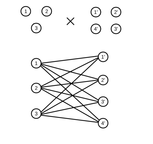
Figure 1: Graph interpretation of the SOAP kernel. Two local environments comprised of 3 and 4 atoms are compared by forming a bipartite graph that links pairs of atoms.

Seeking a graph interpretation of (21), we rewrite it in matrix form,

$$\left\{\begin{array}[]{rl}\displaystyle S(\tilde{x},\tilde{x}^{\prime})&\displaystyle=\sum_{i=1}^{\tilde{n}}\sum_{i^{\prime}=1}^{\tilde{n}^{\prime}}B_{ii^{\prime}}^{2}=\mathrm{Tr}(B^{T}B),\\ \displaystyle B_{ii^{\prime}}&\displaystyle=\sqrt{\omega(z_{i})\omega(z_{i}^{\prime})f_{\mathrm{c}}(|\mathbf{r}_{i}|)f_{\mathrm{c}}(|\mathbf{r}^{\prime}_{i^{\prime}}|)\phi_{\sigma}(|\mathbf{r}_{i}-\mathbf{r}^{\prime}_{i^{\prime}}|)}.\end{array}\right.$$ (23)

The object $B\in\mathbb{R}^{\tilde{n}\times\tilde{n}^{\prime}}$ is suggestive of an adjacency matrix. However, its indices $i$ and $i^{\prime}$ reference atoms from different environments $\tilde{x}$ and $\tilde{x}^{\prime}$. Indeed, the graphical interpretation of $B$ would be bipartite (i.e., containing only cross-links between the atoms of $\tilde{x}$ and $\tilde{x}^{\prime}$) as illustrated in Fig. 1. Note that the elements $B_{ii^{\prime}}$ vary with the relative rotation between $\tilde{x}$ and $\tilde{x}^{\prime}$, and indeed SOAP requires nontrivial integration (10) to achieve rotational invariance.

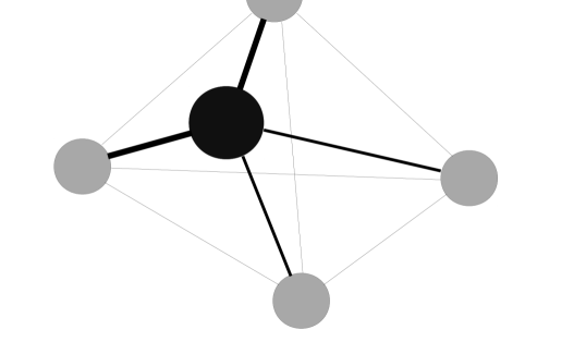
Figure 2: Representation of methane $\mathrm{CH}_{4}$ as a graph. Edge thickness between atoms $i$ and $j$ represents the adjacency matrix element $A_{ij}$.

In GRAPE, we achieve rotational invariance by representing local configurations as graphs. Guided by the form of (23), we introduce an analogous adjacency matrix $A\in\mathbb{R}^{\tilde{n}\times\tilde{n}}$ that operates on a single local environment $\tilde{x}$,

$$A_{ij}=\sqrt{\omega(z_{i})\omega(z_{j})f_{\mathrm{c}}(|\mathbf{r}_{i}|)f_{\mathrm{c}}(|\mathbf{r}_{j}|)\phi_{\sigma}(|\mathbf{r}_{i}-\mathbf{r}_{j}|)}.$$ (24)

For example, Fig. 2 illustrates the graph representation of a methane molecule. The elements $A_{ij}$ of the adjacency matrix (24) link atoms $i$ and $j$, both contained in $\tilde{x}$. Because these elements depend only on pairwise distances, they are manifestly rotation invariant.

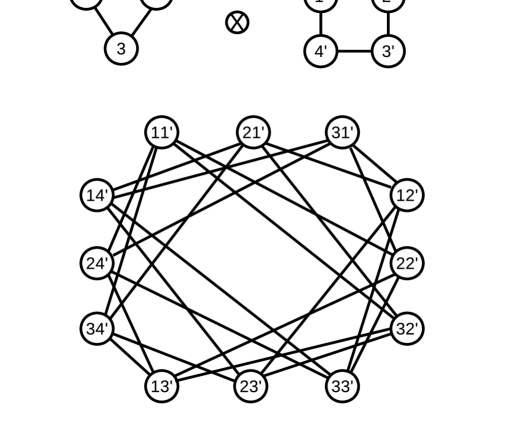
Figure 3: Environments with $3$ and $4$ atoms are graphically represented by adjacency matrices $A$ and $A^{\prime}$. The direct product graph has $3\times 4$ vertices and adjacency matrix elements $(A\otimes A^{\prime})_{ij,kl}=A_{ik}A^{\prime}_{jl}$. Random walk graph kernels operate on this direct product matrix.

To compare two local atomic environments, we apply the exponential graph kernel of Sec. II.3:

$$k(\tilde{x},\tilde{x}^{\prime})=(q^{T}\otimes q^{\prime T})\mathrm{e}^{\gamma A\otimes A^{\prime}}(p\otimes p^{\prime}).$$ (25)

Figure 3 illustrates the graph represented by the direct product matrix, $A\otimes A^{\prime}$, and should be contrasted with Fig. 1. We again use uniform starting and stopping probability distributions $p$, $p^{\prime}$, $q$, $q^{\prime}$ to ensure invariance with respect to permutation of indices, while rotational invariance is naturally inherited from the adjacency matrices $A$ and $A^{\prime}$.

Finally, we use (11) to rescale (25), and (5) to build our model which is suitable for regression on total energies. The kernel is regular and its derivatives are calculable in closed form (Appendix D), so atomic forces are also available from the regression model.

GRAPE shares most of its hyperparameters with SOAP, namely: $\sigma$, $\sigma_{\mathrm{cut}}$, and $\zeta$. However, the SOAP hyperparameter $p$ is replaced by GRAPE’s $\gamma$. Note that $\gamma$ enables effective reweighting of the eigenvalues, each of which corresponds to a different length scale Vishwanathan et al. (2010); Shrivastava and Li (2014a, b). For all methods considered in this work, we must also specify the regularization parameter $\lambda$ used in kernel ridge regression (5).

The computational cost to directly evaluate the local GRAPE kernel $k(\tilde{x},\tilde{x}^{\prime})$ scales as $C_{\mathrm{loc}}\sim\tilde{n}^{3}$ (see Sec. II.3), where $\tilde{n}$ is the typical number of atoms in local environments $\tilde{x}$ and $\tilde{x}^{\prime}$. Global energy regression (5) requires many local kernel evaluations, for both SOAP and GRAPE methods. Evaluating the total kernel (4) requires double summation over all $n\sim n^{\prime}$ atoms in total configurations $x$ and $x^{\prime}$, and thus scales as $\mathcal{O}(n^{2}C_{\mathrm{loc}})$. If there are $N$ atomic configurations $(x_{i})_{i=1\dots N}$ in the dataset, then evaluating the full kernel matrix $K$ scales as $\mathcal{O}(N^{2}n^{2}C_{\mathrm{loc}})$. Matrix inversion brings the total scaling to $\mathcal{O}(N^{2}n^{2}C_{\mathrm{loc}}+N^{3})$. An improvement is to precompute the diagonalization of every local adjacency matrix at cost $\mathcal{O}(Nn\tilde{n}^{3})$. Then subsequent local kernel evaluations scale like $C_{\mathrm{loc}}\sim\tilde{n}^{2}$ and the total cost of building the GRAPE energy regression model becomes $\mathcal{O}(Nn\tilde{n}^{3}+N^{2}n^{2}\tilde{n}^{2}+N^{3})$. Once the model is built, computing the approximation energy (5) for a new configuration scales as $\mathcal{O}(n\tilde{n}^{3}+Nn^{2}\tilde{n}^{2})$.

IV Benchmark

We demonstrate the competitiveness of GRAPE by benchmarking it on a standard energy regression problem. We use the QM7 dataset of organic models used in Ref. Rupp et al., 2012 and freely available at http://quantum-machine.org/datasets/. This database contains $7165$ molecules randomly selected from the GDB-13 database with associated atomization energies, typically between $-2000$ and $-800$ kcal/mol, obtained from hybrid DFT calculations Hohenberg and Kohn (1964); Kohn and Sham (1965). GDB-13 contains approximately $10^{9}$ organic molecules up to $23$ atoms in size, and formed from elements H, C, N, O, and S. QM7 has been randomly partitioned into $5$ sequences, each containing 1433 molecules. We use the first $N$ molecules of Partition 1 as training data (with $N=100,300,500,1,000$), and Partitions 2 and 3 as validation data, i.e. to select the hyperparameters necessary for the various regression methods (discussed below). Finally, after having locked the hyperparameters, we use Partition 4 as our test data, from which we estimate the mean absolute error (MAE) and root mean square error (RMSE) of the energy regression models.

We compare the performance of GRAPE against that of the Coulomb matrix method Rupp et al. (2012) (Appendix C) and SOAP Bartók and Csányi (2015). After experimenting on the validation data, we selected the following hyperparameters for these methods. We set the Gaussian width parameter in (7) to be $\sigma=1.0\,\mbox{\AA}$ for both SOAP and GRAPE. This provides a small overlap of the Gaussian densities of bonded atoms, which are typically separated by a few Å. We select the cutoff radius in (8) to be $R_{\mathrm{cut}}=4.0\,\mbox{\AA}$ for both SOAP and GRAPE, such that a typical local atomic neighborhood contains around 5 atoms. Interestingly, we find that GRAPE is especially sensitive to this hyperparameter, and that the energy regression error would nearly double if we instead selected $R_{\mathrm{cut}}=5.0\,\mbox{\AA}$ for GRAPE. We must also select the weight $\omega(z_{i})$ in (6) and (24) as a function of atomic number $z_{i}$. Again, after some experimentation, we select $\omega(z_{i})=z_{i}$ for SOAP and $\omega(z_{i})=1/z_{i}$ for GRAPE. The latter implies that the GRAPE hyperparameter $\gamma$ appearing in (25) should scale like the square of the typical atomic number in the data; we select $\gamma=40.0$. Consistent with previous work Bartók et al. (2013), we select $p=2$ for SOAP (10) and $\zeta=4.0$ in (11) for both SOAP and GRAPE. We select $\alpha=0.05$ for the Coulomb hyperparameter appearing in Eq. (44). The last hyperparameter $\lambda$, appearing in (5), regularizes the kernel regression. We select $\lambda=10^{-7}$ for Coulomb, $\lambda=10^{-5}$ for SOAP, and $\lambda=10^{-3}$ for GRAPE. In selecting the above hyperparameters, we put approximately equal weight on the MAE and RMSE. We caution that all three models (Coulomb, SOAP, GRAPE) would likely benefit from a more exhaustive search over the hyperparameters. Our results should thus be interpreted as a qualitative comparison of GRAPE’s performance relative to Coulomb and SOAP.

	$N$	100	300	500	1,000
Coulomb	MAE	25.6	19.8	17.9	17.7
	RMSE	50.8	33.5	27.1	28.5
SOAP	MAE	15.6	11.3	10.4	9.7
	RMSE	21.0	15.6	14.5	13.3
GRAPE	MAE	11.2	10.1	9.6	9.0
	RMSE	14.9	13.9	13.3	12.7

Table 1: Mean Absolute Error (MAE) and Root Mean Square Error (RMSE), in units of kcal/mol, for Coulomb, SOAP and GRAPE regression methods, and various sizes $N$ of the training dataset.

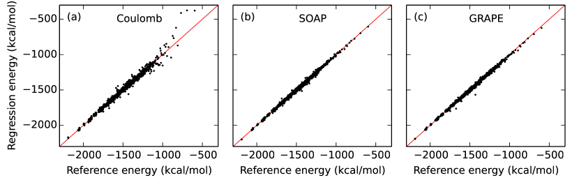
Figure 4: Atomization energies predicted by (a) Coulomb, (b) SOAP, and (c) GRAPE methods. The three regression models were built using a training dataset of $N=1,000$ organic molecules. Reference energies were calculated using density functional theory.

Table 1 displays the MAE and RMSE error estimates for all three methods and various sizes $N$ of the training dataset. Figure 4 shows regression energies for the test data with $N=1,000$, and we observe that GRAPE is competitive with SOAP; given our limited tuning of the hyperparameters, we cannot conclude that one method outperforms the other. However, both SOAP and GRAPE significantly and consistently outperform the Coulomb method. We note that our MAE and RMSE estimates for the Coulomb method are consistent with those previously reported Rupp et al. (2012), when holding $N$ fixed.

For reference, the best known methods in the literature outperform all three kernels in Table 1. Reference Hansen et al., 2013 achieves an MAE of $\approx 6$ kcal/mol for $N=1,000$ using a Laplacian kernel applied to a random sorting of the Coulomb matrix. Montavon et al. (2012) The Bag-of-Bonds kernel method Hansen et al. (2015) reduces the MAE to $\approx 3.3$ for $N=1,000$. Neural networks appear to be state of the art for this QM7 dataset. When training on $N=5,800$ molecules, the Deep Tensor Neural Network Schütt et al. (2017) achieves an MAE of $\approx 1.0$ kcal/mol—a significant improvement over the Bag-of-Bonds MAE, $\approx 1.5$ kcal/mol.

V Discussion

We introduced GRAPE, a simple and flexible method for energy regression based on random walk graph kernels. The approach is invariant with respect to translations, rotations, and permutations of same-species atoms. Using a standard benchmark dataset of organic molecules, we demonstrated that GRAPE’s energy predictions are competitive with commonly applied kernel methods. Because the GRAPE kernel is regular and admits simple closed-form derivatives, it is a candidate for fitting atomic forces, although we did not benchmark the method on this application.

Like the Coulomb method Rupp et al. (2012), GRAPE essentially consists of comparing matrices. These matrices, built upon interatomic distances, are inherently invariant with respect to translation and rotation, while carrying complete information of the system. However, the matrix representation lacks permutation invariance. To restore permutation invariance, the Coulomb method restricts its attention to the list of ordered eigenvalues. Unfortunately, due to this sorting, the associated kernel becomes non-differentiable, which can be a source of instability, as pointed out in Ref. Hirn et al., 2016. Unlike Coulomb, GRAPE is completely regular.

An alternative machine learning approach is to begin by representing the atomic configuration as a density, e.g. using Gaussians peaked on each atomic position. This density field provides a natural way to compare two environments Bartók et al. (2010); Ferré et al. (2015); Hirn et al. (2015), and this is the approach taken by the SOAP method Bartók et al. (2013). A disadvantage of this approach is that the density is not inherently rotational invariant, and density-based kernels typically require an explicit integration over rotations. An achievement of the SOAP kernel is that its rotational integral, Eq. (10), can be evaluated in closed form via a spherical harmonic expansion of the Gaussian densities. GRAPE obviates the need for such an integral in the first place.

An exciting aspect of the GRAPE approach is its flexibility for future extensions. For example, one can use multiscale analysis techniques, such as the multiscale Laplacian graph kernel Kondor and Pan (2016), or wavelet and scattering transforms over graphs Smalter et al. (2009); Hammond et al. (2011); Chen et al. (2014). Another promising research direction is to encode more physical knowledge into the graph, e.g. using labeled graphs Vishwanathan et al. (2010). The vertex labels could directly represent the atomic species, or could more subtly encode chemical information such as the number of electrons in the valence shell.

Appendix A Kernel ridge regression

Here we review the machine learning technique of kernel ridge regression. We assume a dataset of pairs $(x_{i},y_{i})_{i=1\dots N}$. In our application, each $x_{i}$ represents an atomic configuration and $y_{i}$ its corresponding energy. The goal is to build a model of energies $\hat{E}(x)$ for configurations $x$ not contained in the dataset. Following Ref. Hastie et al., 2009 we begin with ordinary ridge regression.

We formally model the energy as a linear combination of descriptors $(h_{m})_{m=1\dots M}$,

$$\hat{E}(x)=\sum_{m=1}^{M}\beta_{m}h_{m}(x),$$ (26)

where $M$ is possibly infinite. Note that $\hat{E}(x)$ is linear in the regression coefficients $\beta_{m}$ but potentially very nonlinear in $x$. We select regression coefficients $\hat{\beta}_{m}$ that minimize a loss function

$$\sum_{i=1}^{N}V(y_{i}-\hat{E}(x_{i}))+\frac{\lambda}{2}\sum_{m=1}^{M}\beta_{m}^{2}.$$ (27)

The simplest error measure, $V(r)=r^{2}$, yields a linear system of equations to be solved for $\beta_{m}$. The solution is the well known ridge regression model Hoerl and Kennard (1970):

$$\hat{E}(x) =\sum_{m=1}^{M}\hat{\beta}_{m}h_{m}(x),$$ (28)

$$\hat{\beta} =(HH^{T}+\lambda I)^{-1}Hy,$$ (29)

with matrix elements $H_{mi}=h_{m}(x_{i})$ and vector $y=(y_{1},y_{2},\dots,y_{N})$. The empirical regularization parameter $\lambda>0$ effectively smooths the approximation $\hat{E}$, and consequently improves the conditioning of the linear inversion problem.

It turns out that we can generalize this model by introducing the inner product kernel,

$$K(x,x^{\prime})=\sum_{m=1}^{M}h_{m}(x)h_{m}(x^{\prime}),$$ (30)

which measures similarity between inputs $x$ and $x^{\prime}$. Note that

$$K_{ij}=K(x_{i},x_{j}) =(H^{T}H)_{i,j},$$ (31)

$$K(x,x_{i}) =(h^{T}H)_{i},$$ (32)

where $h=(h_{1}(x),h_{2}(x),\dots,h_{M}(x))$. The matrix identity $(HH^{T}+\lambda I)^{-1}H=H(H^{T}H+\lambda I)^{-1}$ allows us to rewrite (28) and (29) in the suggestive form:

$$\hat{E}(x) =\sum_{i=1}^{N}\hat{\alpha}_{i}K(x,x_{i}),$$ (33)

$$\hat{\alpha} =(K+\lambda I)^{-1}y.$$ (34)

The key insight is that the descriptors $h_{m}$ no longer appear explicitly. One may select the kernel $K$ directly, and thus implicitly define the family $(h_{m})_{m=1\dots M}$.

Equations (33) and (34) together with a suitable kernel constitute the method of kernel ridge regression. The kernel must be symmetric and positive, i.e. $K(x,x^{\prime})=K(x^{\prime},x)$ for all $x$, $x^{\prime}$, and $\sum_{i}\sum_{i^{\prime}}\alpha_{i}\alpha_{i^{\prime}}K(x_{i},x_{i^{\prime}})\geq 0$ for any non-empty collection of points and coefficients $\{(x_{i},\alpha_{i})\}$. By Mercer’s theorem Mercer (1909), these conditions are equivalent to the decomposition (26).

There are multiple ways to interpret Eqs. (33) and (34). In statistical learning theory, we may derive $\hat{E}(x)$ as the function in some space $\mathcal{H}$ that best minimizes the squared error $\sum_{i=1}^{N}\left(y_{i}-\hat{E}(x_{i})\right)^{2}$ subject to a regularization term $\lambda||\hat{E}||_{\mathcal{H}}$. The kernel $K$ generates both $\mathcal{H}$ (the so-called reproducing kernel Hilbert space) and its norm $||\cdot||_{\mathcal{H}}$ Smola (1998); Scholkopf and Smola (2001). Another interpretation is Bayesian. In this case, one views the coefficients $\beta_{m}$ as independent random variables with Gaussian prior probabilities; then the kernel $K$ specifies the covariance of $y$ and $y^{\prime}$, and $\hat{E}(x)$ becomes the posterior expectation for configuration $x$. This approach is called Gaussian process regression or Kriging Rasmussen and Williams (2006).

We note that Eq. (33) [but not (34)] is independent of the specific choice of error measure $V$. For example, the method of support vector regression corresponds to the choice $V(r)=\max(0,|r|-\epsilon)$.

Appendix B Local energy decomposition

We assume that the energy of an atomic configuration $x$ with $n$ atoms can be decomposed as a sum over local atomic environments $\tilde{x}_{\ell}$,

$$E(x)=\sum_{\ell=1}^{n}\varepsilon(\tilde{x}_{\ell}).$$ (35)

Following Eq. (26), we model local energies $\varepsilon(\tilde{x}_{\ell})$ as a linear combination of abstract descriptors $\tilde{h}_{m}(\tilde{x}_{\ell})$,

$$\hat{\varepsilon}(\tilde{x}_{\ell})=\sum_{m=1}^{M}\beta_{m}\tilde{h}_{m}(\tilde{x}_{\ell}).$$ (36)

After inserting (36) into (35), we observe that the model for total energy

$$\hat{E}(x)=\sum_{\ell=1}^{n}\hat{\varepsilon}(\tilde{x}_{\ell})=\sum_{m=1}^{M}\beta_{m}h_{m}(x),$$ (37)

involves the same coefficients $\beta_{m}$ but new descriptors

$$h_{m}(x)=\sum_{\ell=1}^{n}\tilde{h}_{m}(\tilde{x}_{\ell}).$$ (38)

We assume a dataset $(x_{i},y_{i})_{i=1\dots N}$ containing configurations $x_{i}$ and total energies

$$y_{i}=E(x_{i}).$$ (39)

Again minimizing the cost function of Eq. (27), the kernel ridge regression model of Eqs. (33) and (34) is unchanged. However, the kernel between the full atomic configurations is now constrained. Equations (30) and (38) together imply,

$$K(x,x^{\prime})=\sum_{\ell=1}^{n}\sum_{\ell^{\prime}=1}^{n^{\prime}}\tilde{K}(\tilde{x}_{\ell},\tilde{x}^{\prime}_{\ell^{\prime}}).$$ (40)

where $\tilde{K}(\tilde{x}_{\ell},\tilde{x}^{\prime}_{\ell^{\prime}})=\sum_{m}\tilde{h}_{m}(\tilde{x}_{\ell})\tilde{h}_{m}(\tilde{x}^{\prime}_{\ell^{\prime}}).$

We conclude that the energy decomposition (35) constrains the kernel $K$ to a sum over terms $\tilde{K}$ involving local environments. In “kernelizing” this model, we only require specification of the local kernel $\tilde{K}$; the descriptors $\tilde{h}_{m}$ are implicit and typically infinite in number.

Appendix C Coulomb matrix method

We review the Coulomb matrix method of Ref. Rupp et al., 2012. Here, we elide localized kernel (5) and consider only global atomic configurations $x$ as in Ref. Rupp et al., 2012. Given a configuration with positions and atomic numbers $(\mathbf{r}_{i},z_{i})_{i=1\dots N}$, the Coulomb matrix is

$$M_{i,j}=\left\{\begin{array}[]{cc}\frac{z_{i}z_{j}}{\|r_{i}-r_{j}\|},&i\neq j,\\ 0.5\,z_{i}^{2.4},&i=j.\end{array}\right..$$ (41)

Although the matrix is invariant with respect to translations and rotations of the atomic positions, it is not invariant with respect to permutations of indices. The matrix eigenvalues, however, are permutation invariant. To compare configurations $x$ and $x^{\prime}$ (of size $n$ and $n^{\prime}$, respectively), the Coulomb method compares the lists of eigenvalues ($\lambda_{i}$ and $\lambda^{\prime}_{i}$, respectively), sorted by decreasing magnitude and truncated at length $\min(n,n^{\prime})$. We define normalized eigenvalues,

$$\hat{\lambda}_{i} =\text{$\lambda$}_{i}/||\lambda||,$$ (42)

$$\hat{\lambda}^{\prime}_{i} =\text{$\lambda$}^{\prime}_{i}/||\lambda^{\prime}||,$$ (43)

where $||\lambda||=\sqrt{\sum_{i=1}^{n}\lambda_{i}^{2}}$. Then the Coulomb kernel reads

$$K(x,x^{\prime})=\exp\left[-\alpha\,\sum_{i=1}^{\min(n,n^{\prime})}(\hat{\lambda}_{i}-\hat{\lambda}^{\prime}_{i})^{2}\right],$$ (44)

with $\alpha$ a hyperparameter.

Appendix D Computing forces

Given a regression model for energy, it is often desirable to compute its gradient to obtain a regression model for forces. One motivation is to use machine learned forces within molecular dynamics simulations. Another motivation is that typical datasets (e.g. as generated by ab initio calculations) often contain force information that can aid the energy regression Bartók and Csányi (2015). In either case, the key step is to calculate the derivative $\partial_{\mathbf{r}}K(x,x^{\prime})$ of the kernel $K(x,x^{\prime})$ with respect to some atomic position $\mathbf{r}$ in configuration $x$. Here, we consider the exponential graph kernel (25) used in GRAPE. As before, $A$ and $A^{\prime}$ denote the adjacency matrices of $x$ and $x^{\prime}$ respectively. Assuming $\partial_{\mathbf{r}}A^{\prime}=0$, the gradient of the unscaled kernel is,

$$\partial_{\mathbf{r}}k(x,x^{\prime})=\gamma(q^{T}\otimes q^{\prime T})(\partial_{\mathbf{r}}A\otimes A^{\prime})e^{\gamma A\otimes A^{\prime}}(p\otimes p^{\prime}).$$ (45)

Referring to Eq. (24) we see that the GRAPE adjacency matrix element $A_{ij}$ has a simple functional dependence on positions $\mathbf{r}_{i}$ and $\mathbf{r}_{j}$ (and also an implicit dependence on the central atom position $\mathbf{r}_{\ell}$), and it is thus straightforward to express $\partial_{\mathbf{r}}A$ in closed form. To compute the normalized kernel (11), one also needs:

$$\partial_{\mathbf{r}}k(x,x)=2\gamma(q^{T}\otimes q^{T})(\partial_{\mathbf{r}}A\otimes A)e^{\gamma A\otimes A}(p\otimes p).$$ (46)

References

- Ho and Rabitz (1996) T. Ho and H. Rabitz, J. Chem. Phys. 104, 2584 (1996).
- Bettens and Collins (1999) R. P. A. Bettens and M. A. Collins, J. Chem. Phys. 111, 816 (1999).
- Braams and Bowman (2009) B. J. Braams and J. M. Bowman, Int. Rev. Phys. Chem. 28, 577 (2009).
- Hansen et al. (2013) K. Hansen, G. Montavon, F. Biegler, S. Fazli, M. Rupp, M. Scheffler, O. A. von Lilienfeld, A. Tkatchenko, and K.-R. Müller, J. Chem. Theory Comput. 9, 3404 (2013).
- Rupp et al. (2015) M. Rupp, R. Ramakrishnan, and O. A. von Lilienfeld, J. Phys Chem. Lett. 6, 3309 (2015).
- Bartók and Csányi (2015) A. P. Bartók and G. Csányi, Int. J. Quantum Chem. 115, 1051 (2015).
- Behler (2011) J. Behler, J. Chem. Phys. 134, 074106 (2011).
- Bartók et al. (2013) A. P. Bartók, R. Kondor, and G. Csányi, Phys. Rev. B 87, 184115 (2013).
- Thompson et al. (2015) A. Thompson, L. Swiler, C. Trott, S. Foiles, and G. Tucker, J. Comput. Phys. (2015).
- Behler and Parrinello (2007) J. Behler and M. Parrinello, Phys. Rev. Lett. 98, 146401 (2007).
- Handley and Behler (2014) C. M. Handley and J. Behler, Eur. Phys. J. B 87 (2014).
- Behler (2014) J. Behler, J. Phys.: Condens. Matter 26, 183001 (2014).
- Behler (2015) J. Behler, Int. J. Quantum Chem. 115, 1032 (2015).
- Schütt et al. (2017) K. T. Schütt, F. Arbabzadah, S. Chmiela, K. R. Müller, and A. Tkatchenko, Nat. Commun. 8, 13890 (2017).
- Shapeev (2015) A. V. Shapeev, arXiv preprint arXiv:1512.06054 (2015).
- Hirn et al. (2015) M. Hirn, N. Poilvert, and S. Mallat, arXiv preprint arXiv:1502.02077 (2015).
- Hirn et al. (2016) M. Hirn, S. Mallat, and N. Poilvert, arXiv preprint arXiv:1605.04654 (2016).
- Hofmann et al. (2008) T. Hofmann, B. Schölkopf, and A. J. Smola, Ann. Stat. , 1171 (2008).
- Scholkopf and Smola (2001) B. Scholkopf and A. J. Smola, Learning with kernels: support vector machines, regularization, optimization, and beyond (MIT press, Cambridge, 2001).
- Bartók et al. (2010) A. P. Bartók, M. C. Payne, R. Kondor, and G. Csányi, Phys. Rev. Lett. 104, 136403 (2010).
- Rupp et al. (2012) M. Rupp, A. Tkatchenko, K.-R. Müller, and O. A. von Lilienfeld, Phys. Rev. Lett. 108, 058301 (2012).
- Hansen et al. (2015) K. Hansen, F. Biegler, R. Ramakrishnan, W. Pronobis, O. A. von Lilienfeld, K.-R. Müller, and A. Tkatchenko, J. Phys. Chem. Lett. 6, 2326 (2015).
- Schütt et al. (2014) K. T. Schütt, H. Glawe, F. Brockherde, A. Sanna, K. R. Müller, and E. K. U. Gross, Phys. Rev. B 89, 205118 (2014).
- Li et al. (2015) Z. Li, J. R. Kermode, and A. De Vita, Phys. Rev. Lett. 114, 096405 (2015).
- Ferré et al. (2015) G. Ferré, J.-B. Maillet, and G. Stoltz, J. Chem. Phys. 143, 104114 (2015).
- Gärtner et al. (2002) T. Gärtner, K. Driessens, and J. Ramon, in NIPS Workshop on Unreal Data: Principles of Modeling Nonvectorial Data, Vol. 5 (2002) pp. 49–58.
- Gärtner et al. (2003) T. Gärtner, P. Flach, and S. Wrobel, in Learning theory and kernel machines (Springer, 2003) pp. 129–143.
- Vishwanathan et al. (2010) S. V. N. Vishwanathan, N. N. Schraudolph, R. Kondor, and K. M. Borgwardt, J. Mach. Learn. Res. 11, 1201 (2010).
- Drews (2000) J. Drews, Science 287, 1960 (2000).
- Smola and Kondor (2003) A. J. Smola and R. Kondor, in Learning theory and kernel machines (Springer, 2003) pp. 144–158.
- Borgwardt and Kriegel (2005) K. M. Borgwardt and H.-P. Kriegel, in Fifth IEEE International Conference on Data Mining (IEEE, 2005) pp. 8–.
- Ralaivola et al. (2005) L. Ralaivola, S. J. Swamidass, H. Saigo, and P. Baldi, Neural Networks 18, 1093 (2005).
- Sharan and Ideker (2006) R. Sharan and T. Ideker, Nat. Biotechnol. 24, 427 (2006).
- Schietgat et al. (2008) L. Schietgat, J. Ramon, M. Bruynooghe, and H. Blockeel, in International Conference on Discovery Science (Springer, 2008) pp. 197–209.
- Smalter et al. (2009) A. Smalter, J. Huan, and G. Lushington, J. Bioinform. Comput. Biol. 7, 473 (2009).
- Gaüzere et al. (2012) B. Gaüzere, L. Brun, and D. Villemin, Patt. Recogn. Lett. 33, 2038 (2012).
- Sun (2014) H. Y. Sun, Learning over molecules: representations and kernels, Bachelor’s thesis, Harvard College (2014).
- Mercer (1909) J. Mercer, Philos. Trans. Roy. Soc. London Ser. A 209, 415 (1909).
- Kondor and Borgwardt (2008) R. Kondor and K. M. Borgwardt, in Proceedings of the 25th international conference on Machine learning (ACM, 2008) pp. 496–503.
- Shervashidze et al. (2009) N. Shervashidze, S. Vishwanathan, T. Petri, K. Mehlhorn, and K. M. Borgwardt, in AISTATS, Vol. 5 (2009) pp. 488–495.
- Shrivastava and Li (2014a) A. Shrivastava and P. Li, in Advances in Social Networks Analysis and Mining (IEEE, 2014) pp. 62–71.
- Shrivastava and Li (2014b) A. Shrivastava and P. Li, arXiv preprint arXiv:1404.5214 (2014b).
- Imrich and Klavzar (2000) W. Imrich and S. Klavzar, Product graphs (Wiley, 2000).
- Hohenberg and Kohn (1964) P. Hohenberg and W. Kohn, Phys. Rev. 136, B864 (1964).
- Kohn and Sham (1965) W. Kohn and L. J. Sham, Phys. Rev. 140, A1133 (1965).
- Montavon et al. (2012) G. Montavon, K. Hansen, S. Fazli, M. Rupp, F. Biegler, A. Ziehe, A. Tkatchenko, A. V. Lilienfeld, and K.-R. Müller, in Advances in Neural Information Processing Systems 25, edited by F. Pereira, C. J. C. Burges, L. Bottou, and K. Q. Weinberger (Curran Associates, Inc., 2012) pp. 440–448.
- Kondor and Pan (2016) R. Kondor and H. Pan, arXiv preprint arXiv:1603.06186v2 (2016).
- Hammond et al. (2011) D. K. Hammond, P. Vandergheynst, and R. Gribonval, Appl. Comput. Harm. A. 30, 129 (2011).
- Chen et al. (2014) X. Chen, X. Cheng, and S. Mallat, in Adv. Neural Inf. Process. Syst. (2014) pp. 1709–1717.
- Hastie et al. (2009) T. Hastie, R. Tibshirani, and J. Friedman, “The elements of statistical learning: Data mining, inference, and prediction,” (Springer, New York, 2009) Chap. 12.3.7, pp. 436–437, 2nd ed.
- Hoerl and Kennard (1970) A. E. Hoerl and R. W. Kennard, Technometrics 12, 55 (1970).
- Smola (1998) A. J. Smola, Learning with kernels, Ph.D. thesis, Technische Universität Berlin (1998).
- Rasmussen and Williams (2006) C. E. R. Rasmussen and C. K. I. Williams, Gaussian Processes for Machine Learning (MIT Press, Cambridge, 2006).