Analysis of the mass and width of the $Y(4274)$ as axialvector molecule-like state

Zhi-Gang Wang 111E-mail: zgwang@aliyun.com.

Department of Physics, North China Electric Power University, Baoding 071003, P. R. China

Abstract

In this article, we assign the $Y(4274)$ to be the color octet-octet type axialvector molecule-like state with $J^{PC}=1^{++}$ tentatively, and construct the color octet-octet type axialvector current to study its mass and width with the QCD sum rules in details. The predicted mass favors assigning the $Y(4274)$ to be the color octet-octet type molecule-like state, but the predicted width disfavors assigning the $Y(4274)$ to be the color octet-octet type molecule-like state strongly. The $Y(4274)$ may be the conventional charmonium state $\chi_{c1}(\rm 3P)$, and it is important to observe the decay $Y(4274)\to J/\psi\omega$ to diagnose the nature of the $Y(4274)$.

PACS number: 12.39.Mk, 12.38.Lg

Key words: Molecule-like state, QCD sum rules

1 Introduction

In 2011, the CDF collaboration confirmed the $Y(4140)$ in the $B^{\pm}\rightarrow J/\psi\,\phi K^{\pm}$ decays with a statistical significance greater than $5\,\sigma$, and observed an evidence for a second structure ($Y(4274)$) with approximate significance of $3.1\,\sigma$. The measured mass and width are $\left(4274.4^{+8.4}_{-6.7}\pm 1.9\right)\,\rm{MeV}$ and $\left(32.3^{+21.9}_{-15.3}\pm 7.6\right)\,\rm{MeV}$, respectively [1]. The $Y(4274)$ may be a S-wave $D_{s}\bar{D}_{s0}(2317)+h.c.$ molecular state [2], or not a S-wave $D_{s}\bar{D}_{s0}(2317)+h.c.$ molecular state [3]. In 2013, the CMS collaboration observed an evidence for a second peaking structure besides the $Y(4140)$ with the mass $4313.8\pm 5.3\pm 7.3\,\rm{MeV}$ and width $38^{+30}_{-15}\pm 16\,\rm{MeV}$, respectively [4].

Recently, the LHCb collaboration performed the first full amplitude analysis of the decays $B^{+}\to J/\psi\phi K^{+}$ and confirmed the two old particles $Y(4140)$ and $Y(4274)$ in the $J/\psi\phi$ mass spectrum with statistical significances $8.4\sigma$ and $6.0\sigma$, respectively, and determined the quantum numbers to be $J^{PC}=1^{++}$ with statistical significances $5.7\sigma$ and $5.8\sigma$, respectively [5, 6]. The measured masses and widths are

$\displaystyle Y(4140):M=4146.5\pm 4.5^{+4.6}_{-2.8}\mbox{ MeV}\,,\,\Gamma=83\pm 21^{+21}_{-14}\mbox{ MeV}\,,$
$\displaystyle Y(4274):M=4273.3\pm 8.3^{+17.2}_{-3.6}\mbox{ MeV}\,,\,\Gamma=56\pm 11^{+8}_{-11}\mbox{ MeV}\,.$ (1)

The LHCb collaboration determined the quantum numbers of the $Y(4274)$ to be $J^{PC}=1^{++}$, which rules out the $0^{-+}$ molecule assignment, which is consistent with our previous work [3]. There have been several possible assignments, such as the color sextet-sextet type $cs\bar{c}\bar{s}$ tetraquark state [7, 8], the conventional orbitally excited state $\chi_{c1}(\rm 3P)$ [9], the color triplet-triplet type $\frac{1}{\sqrt{6}}(u\bar{u}+d\bar{d}-2s\bar{s})c\bar{c}$ tetraquark state [10], etc.

In 2014, the Belle collaboration analyzed the $\bar{B}^{0}\to K^{-}\pi^{+}J/\psi$ decays and observed a resonance ($Z_{c}(4200)$) in the $J/\psi\pi^{+}$ invariant mass distribution with a statistical significance of greater than $6.2\,\sigma$, the measured Breit-Wigner mass and width are $M_{Z_{c}(4200)}=4196^{+31}_{-29}{}^{+17}_{-13}\,\rm{MeV}$ and $\Gamma_{Z_{c}(4200)}=370^{+70}_{-70}{}^{+70}_{-132}\,\rm{MeV}$, respectively [11, 12]. The preferred spin-parity is $J^{P}=1^{+}$.

In Ref.[13], we study the axialvector hidden charm and hidden bottom tetraquark states in details with the QCD sum rules and obtain the mass $M_{cu\bar{c}\bar{d},J^{P}=1^{+}}=(4.44\pm 0.19)\,\rm{GeV}$ for the diquark-antidiquark type tetraquark state. In Ref.[14], Chen and Zhu study the vector and axialvector charmonium-like tetraquark states with the QCD sum rules in a systematic way and obtain the mass $M_{cu\bar{c}\bar{d},J^{P}=1^{+}}=(4.16\pm 0.10)\,\rm{GeV}$ for the diquark-antidiquark type tetraquark state. In Ref.[13], we choose the input parameters $m_{c}(\rm 1\,GeV)$, $\langle\bar{q}q\rangle(\rm 1\,GeV)$, ⟨q¯​gs​σ​G​qβŸ©β€‹(1​GeV)delimited-βŸ¨βŸ©Β―π‘žsubscriptπ‘”π‘ πœŽπΊπ‘ž1GeV\langle\bar{q}g_{s}\sigma Gq\rangle(\rm 1\,GeV), while in Ref.[14], Chen and Zhu choose the input parameters $m_{c}(m_{c})$, $\langle\bar{q}q\rangle(\rm 1\,GeV)$, ⟨q¯​gs​σ​G​qβŸ©β€‹(1​GeV)delimited-βŸ¨βŸ©Β―π‘žsubscriptπ‘”π‘ πœŽπΊπ‘ž1GeV\langle\bar{q}g_{s}\sigma Gq\rangle(\rm 1\,GeV). The different predictions for the $C\gamma_{5}\otimes\gamma_{\mu}C$ type axialvector tetraquark state in Ref.[13] and Ref.[14] originate from the different choice of the $c$-quark mass. If we take different choice of the heavy quark masses as a source of uncertainties, the predicted mass is about $M_{cu\bar{c}\bar{d},J^{P}=1^{+}}=(4.06-4.63)\,\rm{GeV}$.

In Ref.[15], we distinguish the charge conjugations of the interpolating currents, study the diquark-antidiquark type axialvector tetraquark states in a systematic way with the QCD sum rules by taking into account the energy scale dependence of the QCD spectral densities for the first time, and obtain the predictions $M_{X(3872)}=3.87^{+0.09}_{-0.09}\,\rm{GeV}$ and $M_{Z_{c}(3900)}=3.91^{+0.11}_{-0.09}\,\rm{GeV}$. In Ref.[16], R. Albuquerque et al take into account the next-to-leading order and next-to-next-to-leading order factorizable radiative corrections to the perturbative terms, and obtain the predication $M_{cu\bar{c}\bar{d},J^{P}=1^{+}}=(3.888\pm 0.130)\,\rm{GeV}$, which also depends on special choice of the energy scale $\mu$, in other words, the $\overline{MS}$ mass $m_{c}(\mu)$. The non-factorizable radiative corrections are still needed to make precise predictions. In leading order approximation, $M_{X(3872)}=3.87^{+0.09}_{-0.09}\,\rm{GeV}$ and $M_{Z_{c}(3900)}=3.91^{+0.11}_{-0.09}\,\rm{GeV}$ [15], after taking into account the next-to-leading order and next-to-next-to-leading order factorizable radiative corrections to the perturbative terms, $M_{cu\bar{c}\bar{d},J^{P}=1^{+}}=(3.888\pm 0.130)\,\rm{GeV}$ [16], the predicted masses only change slightly. On the other hand, including the next-to-leading order and next-to-next-to-leading order factorizable radiative corrections to the perturbative terms leads to the value of the pole residue $\lambda_{cu\bar{c}\bar{d},J^{P}=1^{+}}$ undergoes the replacement $\lambda_{cu\bar{c}\bar{d},J^{P}=1^{+}}\to 1.09\,\lambda_{cu\bar{c}\bar{d},J^{P}=1^{+}}$. According to Refs.[15, 16], the masses of the ground state diquark-antidiquark type axialvector tetraquark states $cu\bar{c}\bar{d}$ are about $3.9\,\rm{GeV}$.

In Ref.[17], Chen et al assign the $Z_{c}(4200)$ to be the ground state axialvector tetraquark state $cu\bar{c}\bar{d}$, calculate its decay width with the QCD sum rules, and obtain the value $\Gamma_{Z_{c}(4200)}=435\pm 180\,\rm{MeV}$. In Ref.[7], Chen et al assign the $X(4140)$ to be the ground state axialvector tetraquark state $cs\bar{c}\bar{s}$. If the $Z_{c}(4200)$ and $X(4140)$ are the color triplet-triplet $C\gamma_{5}\otimes\gamma_{\mu}C$ type axialvector tetraquark states, it is more natural in the case that the $X(4140)$ has larger mass than the $Z_{c}(4200)$.

In Ref.[18], we assign the $Z_{c}(4200)$ to be the color octet-octet type axialvector molecule-like state $\bar{u}\lambda^{a}c\bar{c}\lambda^{a}d$, where $\lambda^{a}$ is the Gell-Mann matrix, and construct the color octet-octet type axialvector current to study its mass (width) with the QCD sum rules by calculating the vacuum condensates up to dimension 10 (5) in the operator product expansion. The predictions $M_{Z_{c}(4200)}=4.19\pm 0.08\,\rm{GeV}$ and $\Gamma_{Z_{c}(4200)}\approx 334\,\rm{MeV}$ are consistent with the experimental data $M_{Z_{c}(4200)}=4196^{+31}_{-29}{}^{+17}_{-13}\,\rm{MeV}$ and $\Gamma_{Z_{c}(4200)}=370^{+70}_{-70}{}^{+70}_{-132}\,\rm{MeV}$ from the Belle collaboration [11, 12], and favor assigning the $Z_{c}(4200)$ to be the color octet-octet type molecule-like state with $J^{PC}=1^{+-}$. Moreover, we study the energy scale dependance of the QCD spectral density of the molecule-like state in details and suggest an empirical energy scale formula to determine the ideal energy scale, in other words, to determine the ideal $c$-quark mass.

Also in Ref.[18], we discuss the possible assignments of the $Z_{c}(3900)$, $Z_{c}(4200)$ and $Z(4430)$ as the ground state color triplet-triplet diquark-antidiquark type tetraquark states with $J^{PC}=1^{+-}$ in details. The QCD sum rules support assigning the $Z_{c}(3900)$ and $Z(4430)$ to be the ground state and the first radial excited state of the diquark-antidiquark type axialvector tetraquark states with $J^{PC}=1^{+-}$, respectively [15, 19]. If we assign the $Z_{c}(4200)$ and $Y(4274)$ to be the molecule-like states with $J^{PC}=1^{+-}$ and $1^{++}$, respectively, the mass difference $M_{Y(4274)}-M_{Z_{c}(4200)}\approx 77\,\rm{MeV}$. It is reasonable, as the $SU(3)$ breaking effects are very small for the four-quark systems [13, 20, 21]. In this article, we assign the $Y(4274)$ to be the color octet-octet type molecule-like state tentatively,

$\displaystyle Y(4274)$ $\displaystyle=$ 12​(π’Ÿsaβ€‹π’ŸΒ―saβ£βˆ—βˆ’π’Ÿsaβ£βˆ—β€‹π’ŸΒ―sa)​(with​   1++),12subscriptsuperscriptπ’Ÿπ‘Žπ‘ superscriptsubscriptΒ―π’Ÿπ‘ π‘Žsuperscriptsubscriptπ’Ÿπ‘ π‘ŽsubscriptsuperscriptΒ―π’Ÿπ‘Žπ‘ withsuperscript1absent\displaystyle\frac{1}{\sqrt{2}}\left({\mathcal{D}}^{a}_{s}\overline{\mathcal{D}}_{s}^{a*}-{\mathcal{D}}_{s}^{a*}\overline{\mathcal{D}}^{a}_{s}\right)\,\,\,({\rm with}\,\,\,1^{++})\,, (2)

study its mass and decay width with the QCD sum rules in details, where the meson-like states π’Ÿsasubscriptsuperscriptπ’Ÿπ‘Žπ‘ {\mathcal{D}}^{a}_{s} and π’Ÿsaβ£βˆ—superscriptsubscriptπ’Ÿπ‘ π‘Ž{\mathcal{D}}_{s}^{a*} have the same quark constituents as the mesons $D_{s}$ and $D_{s}^{*}$ respectively, but they are in the color octet representation, the $a$ corresponds to the Gell-Mann matrix.

The article is arranged as follows: we derive the QCD sum rules for the mass and width of the color octet-octet type axialvector molecule-like state $Y(4274)$ in section 2 and in section 3 respectively; section 4 is reserved for our conclusion.

2 The mass of the color octet-octet type axialvector molecule-like state

In the following, we write down the two-point correlation function Πμ​ν​(p)subscriptΞ πœ‡πœˆπ‘\Pi_{\mu\nu}(p) in the QCD sum rules,

Πμ​ν​(p)subscriptΞ πœ‡πœˆπ‘\displaystyle\Pi_{\mu\nu}(p) $\displaystyle=$ iβ€‹βˆ«d4​x​ei​pβ‹…xβ€‹βŸ¨0|T​{Jμ​(x)​Jν†​(0)}|0⟩,𝑖superscript𝑑4π‘₯superscript𝑒⋅𝑖𝑝π‘₯quantum-operator-product0𝑇subscriptπ½πœ‡π‘₯superscriptsubscriptπ½πœˆβ€ 00\displaystyle i\int d^{4}xe^{ip\cdot x}\langle 0|T\left\{J_{\mu}(x)J_{\nu}^{\dagger}(0)\right\}|0\rangle\,, (3)
$\displaystyle J_{\mu}(x)$ $\displaystyle=$ s¯​(x)​i​γ5​λa​c​(x)​c¯​(x)​γμ​λa​s​(x)βˆ’s¯​(x)​γμ​λa​c​(x)​c¯​(x)​i​γ5​λa​s​(x)2,¯𝑠π‘₯𝑖subscript𝛾5superscriptπœ†π‘Žπ‘π‘₯¯𝑐π‘₯subscriptπ›Ύπœ‡superscriptπœ†π‘Žπ‘ π‘₯¯𝑠π‘₯subscriptπ›Ύπœ‡superscriptπœ†π‘Žπ‘π‘₯¯𝑐π‘₯𝑖subscript𝛾5superscriptπœ†π‘Žπ‘ π‘₯2\displaystyle\frac{\bar{s}(x)i\gamma_{5}\lambda^{a}c(x)\bar{c}(x)\gamma_{\mu}\lambda^{a}s(x)-\bar{s}(x)\gamma_{\mu}\lambda^{a}c(x)\bar{c}(x)i\gamma_{5}\lambda^{a}s(x)}{\sqrt{2}}\,, (4)

where the $\lambda^{a}$ is the Gell-Mann matrix in the color space. We construct the color octet-octet type current $J_{\mu}(x)$ to study the molecule-like state $Y(4274)$. One can consult Refs.[18, 22, 23] for more literatures on the color octet-octet type currents. Under charge conjugation transform $\widehat{C}$, the current $J_{\mu}(x)$ has the property,

$\displaystyle\widehat{C}J_{\mu}(x)\widehat{C}^{-1}$ $\displaystyle=$ $\displaystyle+J_{\mu}(x)\,.$ (5)

At the phenomenological side, we insert a complete set of intermediate hadronic states with the same quantum numbers as the current operator $J_{\mu}(x)$ into the correlation function Πμ​ν​(p)subscriptΞ πœ‡πœˆπ‘\Pi_{\mu\nu}(p) to obtain the hadronic representation [24, 25], and isolate the ground state contribution,

Πμ​ν​(p)subscriptΞ πœ‡πœˆπ‘\displaystyle\Pi_{\mu\nu}(p) $\displaystyle=$ $\displaystyle\frac{\lambda_{Y(4274)}^{2}}{M^{2}_{Y(4274)}-p^{2}}\left(-g_{\mu\nu}+\frac{p_{\mu}p_{\nu}}{p^{2}}\right)+\cdots\,,$ (6)

where the pole residue $\lambda_{Y(4274)}$ is defined by $\langle 0|J_{\mu}(0)|Y(4274)\rangle=\lambda_{Y(4274)}\,\varepsilon_{\mu}$, the $\varepsilon_{\mu}$ is the polarization vector of the axialvector meson $Y(4274)$.

In the following, we briefly outline the operator product expansion for the correlation function Πμ​ν​(p)subscriptΞ πœ‡πœˆπ‘\Pi_{\mu\nu}(p). We contract the quark fields $s$ and $c$ in the correlation function Πμ​ν​(p)subscriptΞ πœ‡πœˆπ‘\Pi_{\mu\nu}(p) with Wick theorem, and obtain the result,

Πμ​ν​(p)subscriptΞ πœ‡πœˆπ‘\displaystyle\Pi_{\mu\nu}(p) $\displaystyle=$ $\displaystyle-\frac{i}{2}\lambda^{a}_{jk}\lambda^{a}_{mn}\lambda^{b}_{k^{\prime}j^{\prime}}\lambda^{b}_{n^{\prime}m^{\prime}}\int d^{4}xe^{ip\cdot x}$ (7)
$\displaystyle\left\{{\rm Tr}\left[\gamma_{5}S_{c}^{kk^{\prime}}(x)\gamma_{5}S^{j^{\prime}j}(-x)\right]{\rm Tr}\left[\gamma_{\mu}S^{nn^{\prime}}(x)\gamma_{\nu}S_{c}^{m^{\prime}m}(-x)\right]\right.$
$\displaystyle+{\rm Tr}\left[\gamma_{\mu}S_{c}^{kk^{\prime}}(x)\gamma_{\nu}S^{j^{\prime}j}(-x)\right]{\rm Tr}\left[\gamma_{5}S^{nn^{\prime}}(x)\gamma_{5}S_{c}^{m^{\prime}m}(-x)\right]$
$\displaystyle-{\rm Tr}\left[\gamma_{\mu}S_{c}^{kk^{\prime}}(x)\gamma_{5}S^{j^{\prime}j}(-x)\right]{\rm Tr}\left[\gamma_{5}S^{nn^{\prime}}(x)\gamma_{\nu}S_{c}^{m^{\prime}m}(-x)\right]$
$\displaystyle\left.-{\rm Tr}\left[\gamma_{5}S_{c}^{kk^{\prime}}(x)\gamma_{\nu}S^{j^{\prime}j}(-x)\right]{\rm Tr}\left[\gamma_{\mu}S^{nn^{\prime}}(x)\gamma_{5}S_{c}^{m^{\prime}m}(-x)\right]\right\}\,,$

where

$\displaystyle S^{ij}(x)$ $\displaystyle=$ i​δi​j​​x2​π2​x4βˆ’Ξ΄i​j​ms4​π2​x2βˆ’Ξ΄i​jβ€‹βŸ¨s¯​s⟩12+i​δi​j​​x​msβ€‹βŸ¨s¯​s⟩48βˆ’Ξ΄i​j​x2β€‹βŸ¨s¯​gs​σ​G​s⟩192+i​δi​j​x2​​x​msβ€‹βŸ¨s¯​gs​σ​G​s⟩1152𝑖subscript𝛿𝑖𝑗π‘₯2superscriptπœ‹2superscriptπ‘₯4subscript𝛿𝑖𝑗subscriptπ‘šπ‘ 4superscriptπœ‹2superscriptπ‘₯2subscript𝛿𝑖𝑗delimited-βŸ¨βŸ©Β―π‘ π‘ 12𝑖subscript𝛿𝑖𝑗π‘₯subscriptπ‘šπ‘ delimited-βŸ¨βŸ©Β―π‘ π‘ 48subscript𝛿𝑖𝑗superscriptπ‘₯2delimited-βŸ¨βŸ©Β―π‘ subscriptπ‘”π‘ πœŽπΊπ‘ 192𝑖subscript𝛿𝑖𝑗superscriptπ‘₯2π‘₯subscriptπ‘šπ‘ delimited-βŸ¨βŸ©Β―π‘ subscriptπ‘”π‘ πœŽπΊπ‘ 1152\displaystyle\frac{i\delta_{ij}\!\not\!{x}}{2\pi^{2}x^{4}}-\frac{\delta_{ij}m_{s}}{4\pi^{2}x^{2}}-\frac{\delta_{ij}\langle\bar{s}s\rangle}{12}+\frac{i\delta_{ij}\!\not\!{x}m_{s}\langle\bar{s}s\rangle}{48}-\frac{\delta_{ij}x^{2}\langle\bar{s}g_{s}\sigma Gs\rangle}{192}+\frac{i\delta_{ij}x^{2}\!\not\!{x}m_{s}\langle\bar{s}g_{s}\sigma Gs\rangle}{1152} (8)
βˆ’i​gs​Gα​βa​ti​ja​(​x​σα​β+σα​β​​x)32​π2​x2βˆ’i​δi​j​x2​​x​gs2β€‹βŸ¨s¯​s⟩27776βˆ’Ξ΄i​j​x4β€‹βŸ¨s¯​sβŸ©β€‹βŸ¨gs2​G​G⟩27648βˆ’18β€‹βŸ¨sΒ―j​σμ​ν​siβŸ©β€‹ΟƒΞΌβ€‹Ξ½π‘–subscript𝑔𝑠subscriptsuperscriptπΊπ‘Žπ›Όπ›½subscriptsuperscriptπ‘‘π‘Žπ‘–π‘—π‘₯superscriptπœŽπ›Όπ›½superscriptπœŽπ›Όπ›½π‘₯32superscriptπœ‹2superscriptπ‘₯2𝑖subscript𝛿𝑖𝑗superscriptπ‘₯2π‘₯superscriptsubscript𝑔𝑠2superscriptdelimited-βŸ¨βŸ©Β―π‘ π‘ 27776subscript𝛿𝑖𝑗superscriptπ‘₯4delimited-βŸ¨βŸ©Β―π‘ π‘ delimited-⟨⟩superscriptsubscript𝑔𝑠2𝐺𝐺2764818delimited-⟨⟩subscript¯𝑠𝑗superscriptπœŽπœ‡πœˆsubscript𝑠𝑖subscriptπœŽπœ‡πœˆ\displaystyle-\frac{ig_{s}G^{a}_{\alpha\beta}t^{a}_{ij}(\!\not\!{x}\sigma^{\alpha\beta}+\sigma^{\alpha\beta}\!\not\!{x})}{32\pi^{2}x^{2}}-\frac{i\delta_{ij}x^{2}\!\not\!{x}g_{s}^{2}\langle\bar{s}s\rangle^{2}}{7776}-\frac{\delta_{ij}x^{4}\langle\bar{s}s\rangle\langle g_{s}^{2}GG\rangle}{27648}-\frac{1}{8}\langle\bar{s}_{j}\sigma^{\mu\nu}s_{i}\rangle\sigma_{\mu\nu}
$\displaystyle-\frac{1}{4}\langle\bar{s}_{j}\gamma^{\mu}s_{i}\rangle\gamma_{\mu}+\cdots\,,$
$\displaystyle S_{c}^{ij}(x)$ $\displaystyle=$ $\displaystyle\frac{i}{(2\pi)^{4}}\int d^{4}ke^{-ik\cdot x}\left\{\frac{\delta_{ij}}{\!\not\!{k}-m_{c}}-\frac{g_{s}G^{n}_{\alpha\beta}t^{n}_{ij}}{4}\frac{\sigma^{\alpha\beta}(\!\not\!{k}+m_{c})+(\!\not\!{k}+m_{c})\sigma^{\alpha\beta}}{(k^{2}-m_{c}^{2})^{2}}\right.$
$\displaystyle\left.+\frac{g_{s}D_{\alpha}G^{n}_{\beta\lambda}t^{n}_{ij}(f^{\lambda\beta\alpha}+f^{\lambda\alpha\beta})}{3(k^{2}-m_{c}^{2})^{4}}-\frac{g_{s}^{2}(t^{a}t^{b})_{ij}G^{a}_{\alpha\beta}G^{b}_{\mu\nu}(f^{\alpha\beta\mu\nu}+f^{\alpha\mu\beta\nu}+f^{\alpha\mu\nu\beta})}{4(k^{2}-m_{c}^{2})^{5}}+\cdots\right\}\,,$
$\displaystyle f^{\lambda\alpha\beta}$ $\displaystyle=$ $\displaystyle(\!\not\!{k}+m_{c})\gamma^{\lambda}(\!\not\!{k}+m_{c})\gamma^{\alpha}(\!\not\!{k}+m_{c})\gamma^{\beta}(\!\not\!{k}+m_{c})\,,$
$\displaystyle f^{\alpha\beta\mu\nu}$ $\displaystyle=$ $\displaystyle(\!\not\!{k}+m_{c})\gamma^{\alpha}(\!\not\!{k}+m_{c})\gamma^{\beta}(\!\not\!{k}+m_{c})\gamma^{\mu}(\!\not\!{k}+m_{c})\gamma^{\nu}(\!\not\!{k}+m_{c})\,,$ (10)

and $t^{n}=\frac{\lambda^{n}}{2}$, $D_{\alpha}=\partial_{\alpha}-ig_{s}G^{n}_{\alpha}t^{n}$ [25], then compute the integrals both in the coordinate space and in the momentum space, and obtain the correlation function Πμ​ν​(p)subscriptΞ πœ‡πœˆπ‘\Pi_{\mu\nu}(p), therefore the QCD spectral density through dispersion relation. For technical details, one can consult Ref.[15].

Now we take the quark-hadron duality below the continuum threshold $s_{0}$ and perform Borel transform with respect to the variable $P^{2}=-p^{2}$ to obtain the QCD sum rule:

Ξ»Y2​exp⁑(βˆ’MY2T2)=∫4​mc2s0𝑑s​ρ​(s)​exp⁑(βˆ’sT2),subscriptsuperscriptπœ†2π‘Œsubscriptsuperscript𝑀2π‘Œsuperscript𝑇2superscriptsubscript4superscriptsubscriptπ‘šπ‘2subscript𝑠0differential-dπ‘ πœŒπ‘ π‘ superscript𝑇2\displaystyle\lambda^{2}_{Y}\,\exp\left(-\frac{M^{2}_{Y}}{T^{2}}\right)=\int_{4m_{c}^{2}}^{s_{0}}ds\,\rho(s)\,\exp\left(-\frac{s}{T^{2}}\right)\,, (11)

where

ρ​(s)πœŒπ‘ \displaystyle\rho(s) $\displaystyle=$ $\displaystyle\rho_{0}(s)+\rho_{3}(s)+\rho_{4}(s)+\rho_{5}(s)+\rho_{6}(s)+\rho_{7}(s)+\rho_{8}(s)+\rho_{10}(s)\,.$ (12)

The explicit expressions of the QCD spectral densities $\rho_{0}(s)$, $\rho_{3}(s)$, $\rho_{4}(s)$, $\rho_{5}(s)$, $\rho_{6}(s)$, $\rho_{7}(s)$, $\rho_{8}(s)$ and $\rho_{10}(s)$ are given in the Appendix. Even in the leading order approximation, the strong coupling constant gs2​(ΞΌ)=4​π​αs​(ΞΌ)superscriptsubscript𝑔𝑠2πœ‡4πœ‹subscriptπ›Όπ‘ πœ‡g_{s}^{2}(\mu)=4\pi\alpha_{s}(\mu) appears according to the equation of motion (Dα​Gβ​α)a=gsβ€‹βˆ‘q=u,d,sq¯​γβ​ta​qsuperscriptsubscript𝐷𝛼subscriptπΊπ›½π›Όπ‘Žsubscript𝑔𝑠subscriptπ‘žπ‘’π‘‘π‘ Β―π‘žsubscript𝛾𝛽superscriptπ‘‘π‘Žπ‘ž\left(D_{\alpha}G_{\beta\alpha}\right)^{a}=g_{s}\sum_{q=u,d,s}\bar{q}\gamma_{\beta}t^{a}q, see the terms gs2β€‹βŸ¨s¯​s⟩2superscriptsubscript𝑔𝑠2superscriptdelimited-βŸ¨βŸ©Β―π‘ π‘ 2g_{s}^{2}\langle\bar{s}s\rangle^{2} in the spectral density $\rho_{6}(s)$. So we have to consider the energy scale dependence of the QCD sum rules, the preferred $c$-quark mass is the $\overline{MS}$ mass $m_{c}(\mu)$.

The on-shell quark propagator has no infrared divergences in perturbation theory, and this provides a perturbative definition of the quark mass [26]. But the pole mass cannot be used to arbitrarily high accuracy because of nonperturbative infrared effects in QCD. The pole mass $\widehat{m}_{c}$ and the $\overline{MS}$ mass $m_{c}(m_{c})$ have the relation,

$\displaystyle\widehat{m}_{c}$ $\displaystyle=$ $\displaystyle m_{c}(m_{c})\left[1+\frac{4}{3}\frac{\alpha_{s}(m_{c})}{\pi}+\cdots\right]\,.$ (13)

The value $m_{c}(m_{c})=1.275\pm 0.025\,\rm{GeV}$ from the Particle Data Group corresponds to $\widehat{m}_{c}=1.67\pm 0.07\,\rm{GeV}$ [27]. If we take the pole mass, then $2\widehat{m}_{c}>M_{J/\psi}>M_{\eta_{c}}$, at the phenomenological side of the QCD sum rules for the $J/\psi$ and $\eta_{c}$,

$\displaystyle\int_{4\widehat{m}_{c}^{2}}^{s_{0}}ds\,f_{J/\psi}^{2}M_{J/\psi}^{2}\,\delta\left(s-M_{J/\psi}^{2}\right)\,\exp\left(-\frac{s}{T^{2}}\right)=0\,,$
$\displaystyle\int_{4\widehat{m}_{c}^{2}}^{s_{0}}ds\,\frac{f_{\eta_{c}}^{2}M_{\eta_{c}}^{2}}{4\widehat{m}_{c}^{2}}\,\delta\left(s-M_{\eta_{c}}^{2}\right)\,\exp\left(-\frac{s}{T^{2}}\right)=0\,.$ (14)

If we want to obtain nonzero values, we have to choose smaller pole mass, $2\widehat{m}_{c}<M_{\eta_{c}}<M_{J/\psi}$ [28]. For an observable particle such as the electron, the physical mass appears as the pole mass, irrespective of the leading order, next-to-leading order, next-to-next-to-leading order, $\cdots$, radiative corrections are concerned. In the leading order approximation, $\widehat{m}_{c}=m_{c}(m_{c})$, however, the $m_{c}(m_{c})$ originates from the radiative corrections and renormalization, which are beyond the leading order approximation. So in the leading order approximation, the definition of the pole mass $\widehat{m}_{c}$ is of arbitrary. Again, we can see that the preferred $c$-quark mass is the $\overline{MS}$ mass $m_{c}(\mu)$. Moreover, the full quark propagator has no pole because the quarks are confined. The pole mass corresponds to a non-confined particle, at the QCD side of the QCD sum rules for $J/\psi$ and $\eta_{c}$, the heavy quarks $c$ and $\bar{c}$ are confined particles.

We derive Eq.(11) with respect to $\tau=\frac{1}{T^{2}}$, then eliminate the pole residue $\lambda_{Y(4274)}$ to obtain the QCD sum rule for the mass,

$\displaystyle M_{Y}^{2}$ $\displaystyle=$ βˆ’βˆ«4​mc2s0𝑑s​dd​τ​ρ​(s)​eβˆ’Ο„β€‹s∫4​mc2s0𝑑s​ρ​(s)​eβˆ’Ο„β€‹s.superscriptsubscript4superscriptsubscriptπ‘šπ‘2subscript𝑠0differential-dπ‘ π‘‘π‘‘πœπœŒπ‘ superscriptπ‘’πœπ‘ superscriptsubscript4superscriptsubscriptπ‘šπ‘2subscript𝑠0differential-dπ‘ πœŒπ‘ superscriptπ‘’πœπ‘ \displaystyle-\frac{\int_{4m_{c}^{2}}^{s_{0}}ds\,\frac{d}{d\tau}\,\rho(s)e^{-\tau s}}{\int_{4m_{c}^{2}}^{s_{0}}ds\rho(s)e^{-\tau s}}\,. (15)

Now we choose the input parameters at the QCD side of the QCD sum rules. We take the vacuum condensates to be the standard values $\langle\bar{q}q\rangle=-(0.24\pm 0.01\,\rm{GeV})^{3}$, ⟨s¯​s⟩=(0.8Β±0.1)β€‹βŸ¨q¯​q⟩delimited-βŸ¨βŸ©Β―π‘ π‘ plus-or-minus0.80.1delimited-βŸ¨βŸ©Β―π‘žπ‘ž\langle\bar{s}s\rangle=(0.8\pm 0.1)\langle\bar{q}q\rangle, ⟨s¯​gs​σ​G​s⟩=m02β€‹βŸ¨s¯​s⟩delimited-βŸ¨βŸ©Β―π‘ subscriptπ‘”π‘ πœŽπΊπ‘ superscriptsubscriptπ‘š02delimited-βŸ¨βŸ©Β―π‘ π‘ \langle\bar{s}g_{s}\sigma Gs\rangle=m_{0}^{2}\langle\bar{s}s\rangle, $m_{0}^{2}=(0.8\pm 0.1)\,\rm{GeV}^{2}$, ⟨αs​G​GΟ€βŸ©=(0.33​GeV)4delimited-⟨⟩subscriptπ›Όπ‘ πΊπΊπœ‹superscript0.33GeV4\langle\frac{\alpha_{s}GG}{\pi}\rangle=(0.33\,\rm{GeV})^{4} at the energy scale $\mu=1\,\rm{GeV}$ [24, 25, 29], and take the $\overline{MS}$ masses $m_{c}(m_{c})=(1.275\pm 0.025)\,\rm{GeV}$ and ms​(ΞΌ=2​GeV)=(0.095Β±0.005)​GeVsubscriptπ‘šπ‘ πœ‡2GeVplus-or-minus0.0950.005GeVm_{s}(\mu=2\,\rm{GeV})=(0.095\pm 0.005)\,\rm{GeV} from the Particle Data Group [27]. Moreover, we take into account the energy-scale dependence of the quark condensate, mixed quark condensate and $\overline{MS}$ masses from the renormalization group equation [27, 30],

⟨s¯​sβŸ©β€‹(ΞΌ)delimited-βŸ¨βŸ©Β―π‘ π‘ πœ‡\displaystyle\langle\bar{s}s\rangle(\mu) $\displaystyle=$ ⟨s¯​sβŸ©β€‹(Q)​[Ξ±s​(Q)Ξ±s​(ΞΌ)]49,delimited-βŸ¨βŸ©Β―π‘ π‘ π‘„superscriptdelimited-[]subscript𝛼𝑠𝑄subscriptπ›Όπ‘ πœ‡49\displaystyle\langle\bar{s}s\rangle(Q)\left[\frac{\alpha_{s}(Q)}{\alpha_{s}(\mu)}\right]^{\frac{4}{9}}\,,
⟨s¯​gs​σ​G​sβŸ©β€‹(ΞΌ)delimited-βŸ¨βŸ©Β―π‘ subscriptπ‘”π‘ πœŽπΊπ‘ πœ‡\displaystyle\langle\bar{s}g_{s}\sigma Gs\rangle(\mu) $\displaystyle=$ ⟨s¯​gs​σ​G​sβŸ©β€‹(Q)​[Ξ±s​(Q)Ξ±s​(ΞΌ)]227,delimited-βŸ¨βŸ©Β―π‘ subscriptπ‘”π‘ πœŽπΊπ‘ π‘„superscriptdelimited-[]subscript𝛼𝑠𝑄subscriptπ›Όπ‘ πœ‡227\displaystyle\langle\bar{s}g_{s}\sigma Gs\rangle(Q)\left[\frac{\alpha_{s}(Q)}{\alpha_{s}(\mu)}\right]^{\frac{2}{27}}\,,
$\displaystyle m_{c}(\mu)$ $\displaystyle=$ mc​(mc)​[Ξ±s​(ΞΌ)Ξ±s​(mc)]1225,subscriptπ‘šπ‘subscriptπ‘šπ‘superscriptdelimited-[]subscriptπ›Όπ‘ πœ‡subscript𝛼𝑠subscriptπ‘šπ‘1225\displaystyle m_{c}(m_{c})\left[\frac{\alpha_{s}(\mu)}{\alpha_{s}(m_{c})}\right]^{\frac{12}{25}}\,,
ms​(ΞΌ)subscriptπ‘šπ‘ πœ‡\displaystyle m_{s}(\mu) $\displaystyle=$ ms​(2​G​e​V)​[Ξ±s​(ΞΌ)Ξ±s​(2​G​e​V)]49,subscriptπ‘šπ‘ 2GeVsuperscriptdelimited-[]subscriptπ›Όπ‘ πœ‡subscript𝛼𝑠2GeV49\displaystyle m_{s}({\rm 2GeV})\left[\frac{\alpha_{s}(\mu)}{\alpha_{s}({\rm 2GeV})}\right]^{\frac{4}{9}}\,,
Ξ±s​(ΞΌ)subscriptπ›Όπ‘ πœ‡\displaystyle\alpha_{s}(\mu) $\displaystyle=$ $\displaystyle\frac{1}{b_{0}t}\left[1-\frac{b_{1}}{b_{0}^{2}}\frac{\log t}{t}+\frac{b_{1}^{2}(\log^{2}{t}-\log{t}-1)+b_{0}b_{2}}{b_{0}^{4}t^{2}}\right]\,,$ (16)

where $t=\log\frac{\mu^{2}}{\Lambda^{2}}$, $b_{0}=\frac{33-2n_{f}}{12\pi}$, $b_{1}=\frac{153-19n_{f}}{24\pi^{2}}$, $b_{2}=\frac{2857-\frac{5033}{9}n_{f}+\frac{325}{27}n_{f}^{2}}{128\pi^{3}}$, $\Lambda=213\,\rm{MeV}$, $296\,\rm{MeV}$ and $339\,\rm{MeV}$ for the flavors $n_{f}=5$, $4$ and $3$, respectively [27].

As the quark masses $m_{c}(\mu)$, ms​(ΞΌ)subscriptπ‘šπ‘ πœ‡m_{s}(\mu), the quark condensate ⟨s¯​sβŸ©β€‹(ΞΌ)delimited-βŸ¨βŸ©Β―π‘ π‘ πœ‡\langle\bar{s}s\rangle(\mu), the mixed condensate ⟨s¯​gs​σ​G​sβŸ©β€‹(ΞΌ)delimited-βŸ¨βŸ©Β―π‘ subscriptπ‘”π‘ πœŽπΊπ‘ πœ‡\langle\bar{s}g_{s}\sigma Gs\rangle(\mu) all depend on the energy scale $\mu$, the QCD spectral density ρ​(s)πœŒπ‘ \rho(s) depends on the energy scale $\mu$, we have to determine the energy scales of the QCD sum rules for those molecule-like states in a consistent way.

The hidden charm (or bottom) four-quark systems $q\bar{q}^{\prime}Q\bar{Q}$ can be described by a double-well potential. In the four-quark system $q\bar{q}^{\prime}Q\bar{Q}$, the heavy quark $Q$ serves as a static well potential and combines with the light quark $q$ to form a heavy diquark $\mathcal{D}^{i}$ in color antitriplet, $q+Q\to\mathcal{D}^{i}$ [15, 19, 20, 21, 31], or combines with the light antiquark $\bar{q}^{\prime}$ to form a heavy meson in color singlet (meson-like state in color octet), $\bar{q}^{\prime}+Q\to\bar{q}^{\prime}Q\,\,(\bar{q}^{\prime}\lambda^{a}Q)$ [18, 23, 32]; the heavy antiquark $\bar{Q}$ serves as another static well potential and combines with the light antiquark $\bar{q}^{\prime}$ to form a heavy antidiquark $\overline{\mathcal{D}}^{i}$ in color triplet, $\bar{q}^{\prime}+\bar{Q}\to\overline{\mathcal{D}}^{i}$ [15, 19, 20, 21, 31], or combines with the light quark $q$ to form a heavy meson in color singlet (meson-like state in color octet), $q+\bar{Q}\to\bar{Q}q\,\,(\bar{Q}\lambda^{a}q)$ [18, 23, 32], where the $i$ is color index, the $\lambda^{a}$ is Gell-Mann matrix. Then

$\displaystyle\mathcal{D}^{i}+\overline{\mathcal{D}}^{i}$ $\displaystyle\to$ $\displaystyle{\rm compact\,\,\,tetraquark\,\,\,states}\,,$
$\displaystyle\bar{q}^{\prime}Q+\bar{Q}q$ $\displaystyle\to$ $\displaystyle{\rm loose\,\,\,molecular\,\,\,states}\,,$
$\displaystyle\bar{q}^{\prime}\lambda^{a}Q+\bar{Q}\lambda^{a}q$ $\displaystyle\to$ $\displaystyle{\rm molecule-like\,\,\,states}\,,$ (17)

the two heavy quarks $Q$ and $\bar{Q}$ stabilize the four-quark systems $q\bar{q}^{\prime}Q\bar{Q}$, just as in the case of the $(\mu^{-}e^{+})(\mu^{+}e^{-})$ molecule in QED [33].

The four-quark systems $q\bar{q}^{\prime}Q\bar{Q}$ are characterized by the effective heavy quark mass ${\mathbb{M}}_{Q}$ and the virtuality $V=\sqrt{M^{2}_{X/Y/Z}-(2{\mathbb{M}}_{Q})^{2}}$ [15, 18, 19, 20, 21, 23, 31, 32]. It is natural to take the energy scale $\mu=V$. The ${\mathbb{M}}_{Q}$ is just an empirical parameter to determine the optimal energy scales of the QCD spectral densities, and has no relation to the pole mass $\hat{m}_{Q}$ or the $\overline{MS}$ mass $m_{Q}(\mu)$.

In Refs.[15, 18, 19, 20, 21, 23, 31, 32], we observe that there exist three universal values for the effective heavy quark masses ${\mathbb{M}}_{Q}$, which correspond to the compact tetraquark states, molecular states, molecule-like states, respectively. The empirical energy scale formula $\mu=\sqrt{M^{2}_{X/Y/Z}-(2{\mathbb{M}}_{Q})^{2}}$ works well in assigning the $X(3872)$, $Z_{c}(3900)$, $Y(3915)$, $Z_{c}(4020/4025)$, $Y(4140)$, $Z_{c}(4200)$, $Y(4260)$, $Y(4360)$, $Z_{c}(4430)$, $X(4500)$, $Y(4630/4660)$, $X(4700)$, $Z_{b}(10610)$, $Z_{b}(10650)$, etc.

We evolve all the input parameters in the QCD spectral density to the special energy scale determined by the empirical formula,

$\displaystyle\mu$ $\displaystyle=$ $\displaystyle\sqrt{M^{2}_{X/Y/Z}-(2{\mathbb{M}}_{c})^{2}}\,.$ (18)

In Ref.[18], we obtain the effective mass ${\mathbb{M}}_{c}=1.98\,\rm{GeV}$ for the molecule-like states. Then we re-checked the numerical calculations and corrected a small error concerning the mixed condensate, the updated value is ${\mathbb{M}}_{c}=2.01\,\rm{GeV}$. From the empirical energy scale formula, we can obtain the energy scale $\mu=1.45\,\rm{GeV}$. After taking into account the $SU(3)$ symmetry breaking effect msβˆ’mu/dβ‰ˆ0.1​GeVsubscriptπ‘šπ‘ subscriptπ‘šπ‘’π‘‘0.1GeVm_{s}-m_{u/d}\approx 0.1\,\rm{GeV}, we obtain the optimal energy scale $\mu=1.25\,\rm{GeV}$ for the QCD spectral density ρ​(s)πœŒπ‘ \rho(s). If we neglect the $SU(3)$ symmetry breaking effect, the effective $c$-quark mass ${\mathbb{M}}_{c}$ can be taken as ${\mathbb{M}}_{c}=2.04\,\rm{GeV}$.

Now we search for the Borel parameter $T^{2}$ and continuum threshold parameter $s_{0}$ to satisfy the following three criteria:

$\bf{1_{\cdot}}$ Pole dominance at the phenomenological side;

$\bf{2_{\cdot}}$ Convergence of the operator product expansion;

$\bf{3_{\cdot}}$ Appearance of the Borel platforms.

The resulting Borel parameter and continuum threshold parameter are $T^{2}=(3.1-3.5)\,\rm{GeV}^{2}$ and $\sqrt{s_{0}}=(4.8\pm 0.1)\,\rm{GeV}$, respectively. At the Borel window, the pole contribution is about $(41-62)\%$, the contributions of the vacuum condensates of dimension 8 and 10 are about $|D_{8}|=(5-7)\%$ and $D_{10}<1\%$, respectively, the first two criteria are satisfied.

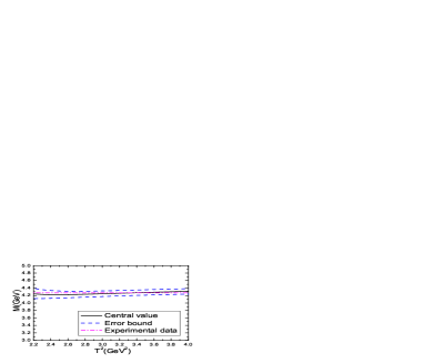
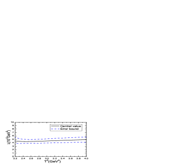
We take into account all uncertainties of the input parameters, and obtain the values of the mass and pole residue, which are shown explicitly in Fig.1,

$\displaystyle M_{Y(4274)}$ $\displaystyle=$ $\displaystyle(4.27\pm 0.09)\,\rm{GeV}\,,$
$\displaystyle\lambda_{Y(4274)}$ $\displaystyle=$ $\displaystyle(4.67\pm 0.74)\times 10^{-2}\,\rm{GeV}^{5}\,.$ (19)

In Fig.1, we plot the mass and pole residue of the $Y(4274)$ with variation of the Borel parameter $T^{2}$ at a larger interval than the Borel window. From the figure, we can see that there appear platforms, the criterion $\bf{3}$ is also satisfied. Now the three criteria are all satisfied, it is reliable to extract the ground state mass. The predicted mass $M_{Y(4274)}=(4.27\pm 0.09)\,\rm{GeV}$ is consistent with the experimental value $4273.3\pm 8.3^{+17.2}_{-3.6}\mbox{ MeV}$ from the LHCb collaboration [5, 6], which supports assigning the $Y(4274)$ to be the color octet-octet type s¯​λa​c​c¯​λa​s¯𝑠superscriptπœ†π‘Žπ‘Β―π‘superscriptπœ†π‘Žπ‘ \bar{s}\lambda^{a}c\bar{c}\lambda^{a}s molecule-like state.

In Ref.[16], R. Albuquerque et al study the hidden-charm and hidden-bottom molecular states and tetraquark states by taking into account the next-to-leading order and next-to-next-to-leading order radiative corrections to the preturbative terms from the factorizable Feynman diagrams (without including the non-factorizable Feynman diagrams). The numerical results indicate that the predicted masses are slightly modified, while the decay constants (which relate to the pole residues) are modified significantly, the largest modification amounts to multiplying the decay constants by a factor $1.8$. So we expect that the predication $M_{Y(4274)}=(4.27\pm 0.09)\,\rm{GeV}$ survives approximately even if the next-to-leading order radiative corrections to the preturbative terms are taken into account. Moreover, at the present time, even the next-to-leading order factorizable contributions are not available for the color octet-octet type molecule-like states, it is a challenging work to calculate both the next-to-leading order factorizable and non-factorizable Feynman diagrams.

Refer to caption
Refer to caption
Figure 1: The mass and pole residue of the $M_{Y(4274)}$ with variation of the Borel parameter $T^{2}$.

3 The width of the color octet-octet type axialvector molecule-like state

We can study the strong decay $Y(4274)\to J/\psi\phi$ with the three-point correlation function Πα​μ​ν​(p,q)subscriptΞ π›Όπœ‡πœˆπ‘π‘ž\Pi_{\alpha\mu\nu}(p,q),

Πα​μ​ν​(p,q)subscriptΞ π›Όπœ‡πœˆπ‘π‘ž\displaystyle\Pi_{\alpha\mu\nu}(p,q) $\displaystyle=$ $\displaystyle i^{2}\int d^{4}xd^{4}ye^{ipx}e^{iqy}\langle 0|T\left\{J_{\alpha}^{J/\psi}(x)J_{\mu}^{\phi}(y)J_{\nu}(0)\right\}|0\rangle\,,$ (20)

where the currents

$\displaystyle J_{\alpha}^{J/\psi}(x)$ $\displaystyle=$ $\displaystyle\bar{c}(x)\gamma_{\alpha}c(x)\,,$
$\displaystyle J_{\mu}^{\phi}(x)$ $\displaystyle=$ s¯​(y)​γμ​s​(y),¯𝑠𝑦subscriptπ›Ύπœ‡π‘ π‘¦\displaystyle\bar{s}(y)\gamma_{\mu}s(y)\,, (21)

interpolate the mesons $J/\psi$ and $\phi(1020)$ according to the current-hadron couplings,

$\displaystyle\langle 0|J_{\alpha}^{J/\psi}(0)|J/\psi(p)\rangle$ $\displaystyle=$ $\displaystyle f_{J/\psi}M_{J/\psi}\xi_{\alpha}\,\,,$
$\displaystyle\langle 0|J_{\mu}^{\phi}(0)|\phi(q)\rangle$ $\displaystyle=$ $\displaystyle f_{\phi}M_{\phi}\zeta_{\mu}\,\,,$ (22)

the $f_{J/\psi}$ and $f_{\phi}$ are the decay constants, the $\xi_{\alpha}$ and $\zeta_{\mu}$ are polarization vectors of the mesons $J/\psi$ and $\phi(1020)$, respectively.

At the phenomenological side, we insert a complete set of intermediate hadronic states with the same quantum numbers as the current operators $J_{\alpha}^{J/\psi}(x)$, $J_{\mu}^{\phi}(y)$, $J_{\nu}(0)$ into the three-point correlation function Πα​μ​ν​(p,q)subscriptΞ π›Όπœ‡πœˆπ‘π‘ž\Pi_{\alpha\mu\nu}(p,q) and isolate the ground state contributions to obtain the result,

Πα​μ​ν​(p,q)subscriptΞ π›Όπœ‡πœˆπ‘π‘ž\displaystyle\Pi_{\alpha\mu\nu}(p,q) $\displaystyle=$ $\displaystyle\frac{f_{\phi}M_{\phi}f_{J/\psi}M_{J/\psi}\lambda_{Y}G_{YJ/\psi\phi}}{(M_{Y}^{2}-p^{\prime 2})(M_{J/\psi}^{2}-p^{2})(M_{\phi}^{2}-q^{2})}\,\varepsilon^{\lambda\tau\rho\theta}p^{\prime}_{\lambda}\left(-g_{\nu\tau}+\frac{p_{\nu}^{\prime}p^{\prime}_{\tau}}{p^{\prime 2}}\right)\left(-g_{\alpha\rho}+\frac{p_{\alpha}p_{\rho}}{p^{2}}\right)$ (23)
$\displaystyle\left(-g_{\mu\theta}+\frac{q_{\mu}q_{\theta}}{q^{2}}\right)+\cdots$
$\displaystyle=$ $\displaystyle\left\{\frac{f_{\phi}M_{\phi}f_{J/\psi}M_{J/\psi}\lambda_{Y}G_{YJ/\psi\phi}}{(M_{Y}^{2}-p^{\prime 2})(M_{J/\psi}^{2}-p^{2})(M_{\phi}^{2}-q^{2})}+\frac{1}{(M_{Y}^{2}-p^{\prime 2})(M_{J/\psi}^{2}-p^{2})}\int_{s^{0}_{\phi}}^{\infty}dt\frac{\rho_{Y\phi}(p^{2},t,p^{\prime 2})}{t-q^{2}}\right.$
$\displaystyle\left.+\frac{1}{(M_{Y}^{2}-p^{\prime 2})(M_{\phi}^{2}-q^{2})}\int_{s^{0}_{J/\psi}}^{\infty}dt\frac{\rho_{YJ/\psi}(t,q^{2},p^{\prime 2})}{t-p^{2}}+\cdots\right\}\left(\varepsilon_{\alpha\mu\nu\lambda}p^{\lambda}+\cdots\right)+\cdots$
$\displaystyle=$ $\displaystyle\left\{\frac{f_{\phi}M_{\phi}f_{J/\psi}M_{J/\psi}\lambda_{Y}G_{YJ/\psi\phi}}{(M_{Y}^{2}-p^{\prime 2})(M_{J/\psi}^{2}-p^{2})(M_{\phi}^{2}-q^{2})}+\frac{C_{Y\phi}}{(M_{Y}^{2}-p^{\prime 2})(M_{J/\psi}^{2}-p^{2})}\right.$
$\displaystyle\left.+\frac{C_{YJ/\psi}}{(M_{Y}^{2}-p^{\prime 2})(M_{\phi}^{2}-q^{2})}+\cdots\right\}\left(\varepsilon_{\alpha\mu\nu\lambda}p^{\lambda}+\cdots\right)+\cdots\,,$

where $p^{\prime}=p+q$, the $G_{YJ/\psi\phi}$ is the hadronic coupling constant, which is defined by

$\displaystyle\langle J/\psi(p,\xi)\phi(q,\zeta)|Y(p^{\prime},\varepsilon)\rangle$ $\displaystyle=$ $\displaystyle iG_{YJ/\psi\phi}\,\varepsilon^{\lambda\tau\rho\theta}p^{\prime}_{\lambda}\varepsilon_{\tau}\xi_{\rho}\zeta_{\theta}\,.$ (24)

In this article, we choose the tensor structure $\varepsilon_{\alpha\mu\nu\lambda}p^{\lambda}$ to study the coupling constant $G_{YJ/\psi\phi}$.

The two unknown functions $\rho_{Y\phi}(p^{2},t,p^{\prime 2})$ and $\rho_{YJ/\psi}(t,q^{2},p^{\prime 2})$ parameterize transitions between the ground states and the higher resonances or the continuum states, the net effects can be parameterized by $C_{Y\phi}$ and $C_{YJ/\psi}$,

$\displaystyle C_{Y\phi}$ $\displaystyle=$ $\displaystyle\int_{s^{0}_{\phi}}^{\infty}dt\frac{\rho_{Y\phi}(p^{2},t,p^{\prime 2})}{t-q^{2}}\,,$
$\displaystyle C_{YJ/\psi}$ $\displaystyle=$ $\displaystyle\int_{s^{0}_{J/\psi}}^{\infty}dt\frac{\rho_{YJ/\psi}(t,q^{2},p^{\prime 2})}{t-p^{2}}\,.$ (25)

In calculations, we take the $C_{Y\phi}$ and $C_{YJ/\psi}$ as free parameters, and vary them to eliminate the contaminations to obtain Borel platforms [34].

We carry out the operator product expansion up to the vacuum condensates of dimension 5 and neglect the gluon condensate, which plays a minor important role. We obtain the QCD spectral density through dispersion relation, take the quark-hadron duality below the continuum thresholds, then set $p^{\prime 2}=p^{2}$ and take double Borel transform with respect to the variables $P^{2}=-p^{2}$ and $Q^{2}=-q^{2}$ respectively to obtain the QCD sum rule,

$\displaystyle\frac{f_{\phi}M_{\phi}f_{J/\psi}M_{J/\psi}\lambda_{Y}G_{YJ/\psi\phi}}{M_{Y}^{2}-M_{J/\psi}^{2}}\left[\exp\left(-\frac{M_{J/\psi}^{2}}{T_{1}^{2}}\right)-\exp\left(-\frac{M_{Y}^{2}}{T_{1}^{2}}\right)\right]\exp\left(-\frac{M_{\phi}^{2}}{T_{2}^{2}}\right)$
$\displaystyle+C_{YJ/\psi}\exp\left(-\frac{M_{Y}^{2}}{T_{1}^{2}}-\frac{M_{\phi}^{2}}{T_{2}^{2}}\right)$
=βˆ’16​2​π4β€‹βˆ«4​mc2sY0𝑑sβ€‹βˆ«0sΟ•0𝑑u​u​1βˆ’4​mc2s​(mcβˆ’ms2βˆ’ms​mc2s)​exp⁑(βˆ’sT12βˆ’uT22)absent162superscriptπœ‹4superscriptsubscript4superscriptsubscriptπ‘šπ‘2subscriptsuperscript𝑠0π‘Œdifferential-d𝑠superscriptsubscript0subscriptsuperscript𝑠0italic-Ο•differential-d𝑒𝑒14superscriptsubscriptπ‘šπ‘2𝑠subscriptπ‘šπ‘subscriptπ‘šπ‘ 2subscriptπ‘šπ‘ superscriptsubscriptπ‘šπ‘2𝑠𝑠superscriptsubscript𝑇12𝑒superscriptsubscript𝑇22\displaystyle=-\frac{1}{6\sqrt{2}\pi^{4}}\int_{4m_{c}^{2}}^{s^{0}_{Y}}ds\int_{0}^{s^{0}_{\phi}}duu\sqrt{1-\frac{4m_{c}^{2}}{s}}\left(m_{c}-\frac{m_{s}}{2}-\frac{m_{s}m_{c}^{2}}{s}\right)\exp\left(-\frac{s}{T_{1}^{2}}-\frac{u}{T_{2}^{2}}\right)
+4​ms​mcβ€‹βŸ¨s¯​s⟩3​2​π2β€‹βˆ«4​mc2sY0𝑑s​1βˆ’4​mc2s​exp⁑(βˆ’sT12)4subscriptπ‘šπ‘ subscriptπ‘šπ‘delimited-βŸ¨βŸ©Β―π‘ π‘ 32superscriptπœ‹2superscriptsubscript4superscriptsubscriptπ‘šπ‘2subscriptsuperscript𝑠0π‘Œdifferential-d𝑠14superscriptsubscriptπ‘šπ‘2𝑠𝑠superscriptsubscript𝑇12\displaystyle+\frac{4m_{s}m_{c}\langle\bar{s}s\rangle}{3\sqrt{2}\pi^{2}}\int_{4m_{c}^{2}}^{s^{0}_{Y}}ds\sqrt{1-\frac{4m_{c}^{2}}{s}}\exp\left(-\frac{s}{T_{1}^{2}}\right)
βˆ’2β€‹βŸ¨s¯​gs​σ​G​s⟩27​2​π2β€‹βˆ«4​mc2sY0𝑑s​1βˆ’4​mc2s​s+2​mc2s​exp⁑(βˆ’sT12)2delimited-βŸ¨βŸ©Β―π‘ subscriptπ‘”π‘ πœŽπΊπ‘ 272superscriptπœ‹2superscriptsubscript4superscriptsubscriptπ‘šπ‘2subscriptsuperscript𝑠0π‘Œdifferential-d𝑠14superscriptsubscriptπ‘šπ‘2𝑠𝑠2superscriptsubscriptπ‘šπ‘2𝑠𝑠superscriptsubscript𝑇12\displaystyle-\frac{2\langle\bar{s}g_{s}\sigma Gs\rangle}{27\sqrt{2}\pi^{2}}\int_{4m_{c}^{2}}^{s^{0}_{Y}}ds\sqrt{1-\frac{4m_{c}^{2}}{s}}\frac{s+2m_{c}^{2}}{s}\exp\left(-\frac{s}{T_{1}^{2}}\right)
βˆ’ms​mcβ€‹βŸ¨s¯​gs​σ​G​s⟩9​2​π2​T22β€‹βˆ«4​mc2sY0𝑑s​1βˆ’4​mc2s​exp⁑(βˆ’sT12),subscriptπ‘šπ‘ subscriptπ‘šπ‘delimited-βŸ¨βŸ©Β―π‘ subscriptπ‘”π‘ πœŽπΊπ‘ 92superscriptπœ‹2superscriptsubscript𝑇22superscriptsubscript4superscriptsubscriptπ‘šπ‘2subscriptsuperscript𝑠0π‘Œdifferential-d𝑠14superscriptsubscriptπ‘šπ‘2𝑠𝑠superscriptsubscript𝑇12\displaystyle-\frac{m_{s}m_{c}\langle\bar{s}g_{s}\sigma Gs\rangle}{9\sqrt{2}\pi^{2}T_{2}^{2}}\int_{4m_{c}^{2}}^{s^{0}_{Y}}ds\sqrt{1-\frac{4m_{c}^{2}}{s}}\exp\left(-\frac{s}{T_{1}^{2}}\right)\,, (26)

where the $s^{0}_{Y}$ and $s^{0}_{\phi}$ are the continuum threshold parameters for the $Y(4274)$ and $\phi(1020)$, respectively.

The hadronic parameters are taken as $M_{\phi}=1.019461\,\rm{GeV}$, $M_{J/\psi}=3.0969\,\rm{GeV}$ [27], $f_{J/\psi}=0.418\,\rm{GeV}$ [35], $f_{\phi}=0.253\,\rm{GeV}$, $\sqrt{s^{0}_{\phi}}=1.5\,\rm{GeV}$, $\sqrt{s^{0}_{Y}}=4.8\,\rm{GeV}$, $M_{Y}=4.268\,\rm{GeV}$, $\lambda_{Y}=4.674\times 10^{-2}\,\rm{GeV}^{5}$, $T_{1}^{2}=(3.1-3.5)\,\rm{GeV}^{2}$, $T_{2}^{2}=(2.9-3.3)\,\rm{GeV}^{2}$ (present work). The unknown parameter is chosen as $C_{YJ/\psi}=0.037\,\rm{GeV}^{7}$ to obtain platforms in the Borel windows $T_{1}^{2}=(3.1-3.5)\,\rm{GeV}^{2}$ and $T_{2}^{2}=(2.9-3.3)\,\rm{GeV}^{2}$. The input parameters at the QCD side are chosen as the same in the two-point QCD sum rules for the $Y(4274)$.

Refer to caption
Refer to caption
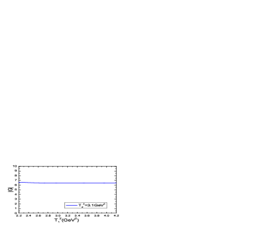
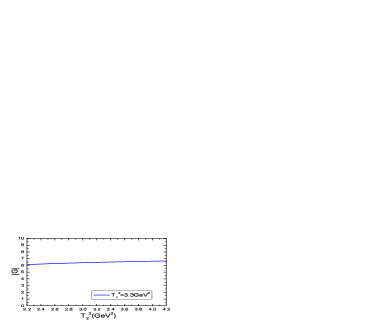
Figure 2: The hadronic coupling constant $G_{YJ/\psi\phi}$ with variations of the Borel parameters $T^{2}_{1}$ and $T_{2}^{2}$, respectively.

In Fig.2, we plot the hadronic coupling constant $G_{YJ/\psi\phi}$ with variations of the Borel parameters $T^{2}_{1}$ and $T_{2}^{2}$, respectively. From the figure, we can see that there appear platforms in the Borel windows $T_{1}^{2}=(3.1-3.5)\,\rm{GeV}^{2}$ and $T_{2}^{2}=(2.9-3.3)\,\rm{GeV}^{2}$, respectively. The central value of the hadronic coupling constant $G_{YJ/\psi\phi}$ is

$\displaystyle G_{YJ/\psi\phi}$ $\displaystyle=$ $\displaystyle-6.43\,.$ (27)

If the radiative corrections to the perturbative term of the correlation function Πα​μ​ν​(p,q)subscriptΞ π›Όπœ‡πœˆπ‘π‘ž\Pi_{\alpha\mu\nu}(p,q) also amount to multiplying a factor about $1.8$, as the color octet-octet type current $J_{\mu}(x)$ is also presented, the value of the quantity $f_{\phi}\,f_{J/\psi}\,\lambda_{Y}\,G_{YJ/\psi\phi}$ at the hadronic side in the QCD sum rules in Eq.(26) changes according to the rule,

$\displaystyle f_{\phi}\,f_{J/\psi}\,\lambda_{Y}\,G_{YJ/\psi\phi}$ $\displaystyle\to$ $\displaystyle f_{\phi}\,f_{J/\psi}\,\lambda_{Y}\,G_{YJ/\psi\phi}\times 1.8\,.$ (28)

In this article, we take the values $f_{J/\psi}=0.418\,\rm{GeV}$ [35] and $f_{\phi}=0.253\,\rm{GeV}$, which include next-to-leading order radiative corrections. The factors $1.8$ come from the radiative corrections to the two-point correction function and three-point correlation function cancel out with each other, the net modification of the hadronic coupling constant $G_{YJ/\psi\phi}$ is estimated to be tiny, just like the hadronic coupling constants $D^{*}D\pi$ and $B^{*}B\pi$, the net effects of the radiative corrections can be neglected [36].

Now it is easy to obtain the decay width,

$\displaystyle\Gamma(Y(4274)\to J/\psi\phi)$ $\displaystyle=$ $\displaystyle\frac{p\left(M_{Y},M_{J/\psi},M_{\phi}\right)}{24\pi M_{Y}^{2}}G_{YJ/\psi\phi}^{2}\left\{\frac{\left(M_{Y}^{2}-M_{\phi}^{2}\right)^{2}}{2M_{J/\psi}^{2}}+\frac{\left(M_{Y}^{2}-M_{J/\psi}^{2}\right)^{2}}{2M_{\phi}^{2}}\right.$ (29)
$\displaystyle\left.+4M_{Y}^{2}-\frac{M_{J/\psi}^{2}+M_{\phi}^{2}}{2}\right\}$
$\displaystyle=$ 1.8​GeV≫56Β±11βˆ’11+8​ MeV​Experimental​value​[5, 6],much-greater-than1.8GeVplus-or-minus56subscriptsuperscript11811Β MeVExperimentalvalue[5, 6]\displaystyle 1.8\,{\rm{GeV}}\gg 56\pm 11^{+8}_{-11}{\mbox{ MeV}}\,\,\,\rm{Experimental\,\,\,value}\,\,\cite[cite]{[\@@bibref{}{LHCb-4500-1606.07895,LHCb-4500-1606.07898}{}{}]}\,,

where $p(a,b,c)=\frac{\sqrt{[a^{2}-(b+c)^{2}][a^{2}-(b-c)^{2}]}}{2a}$. It is difficult to assign the $Y(4274)$ to be the color octet-octet type molecule-like state s¯​λa​c​c¯​λa​s¯𝑠superscriptπœ†π‘Žπ‘Β―π‘superscriptπœ†π‘Žπ‘ \bar{s}\lambda^{a}c\bar{c}\lambda^{a}s. In Ref.[20], we assign the $Y(4140)$ to be the diquark-antidiquark type tetraquark state $cs\bar{c}\bar{s}$ with $J^{PC}=1^{++}$, and study the mass and pole residue with the QCD sum rules in details. The predicted mass disfavors assigning the $Y(4140)$ to be the $J^{PC}=1^{++}$ diquark-antidiquark type tetraquark state $cs\bar{c}\bar{s}$. The $Y(4140)$ and $Y(4274)$ have the same quantum numbers except for the masses and widths, the QCD sum rules also disfavor assigning the $Y(4274)$ to be the $J^{PC}=1^{++}$ diquark-antidiquark type tetraquark state $cs\bar{c}\bar{s}$.

The mass of the $\chi_{c1}(\rm 3P)$ state is $4271\,\rm{MeV}$ and $4317\,\rm{MeV}$ from the non-relativistic potential model and the relativized Godfrey-Isgur model respectively [37], which are consistent with the experimental value $4273.3\pm 8.3^{+17.2}_{-3.6}\mbox{ MeV}$ from the LHCb collaboration [5, 6]. The width of the $\chi_{c1}(\rm 3P)$ state is $39\,\rm{MeV}$ from the non-relativistic potential model [37], which is consistent with the experimental value $56\pm 11^{+8}_{-11}{\mbox{ MeV}}$ from the LHCb collaboration [5, 6]. The $Y(4274)$ may be the conventional charmonium $\chi_{c1}(\rm 3P)$ state [9], while in Ref.[38], the $Y(4140)$ is assigned to the $\chi_{c1}(\rm 3P)$ state. In Ref.[39], we study the vector meson transitions among the charmonium and bottomonium states with the heavy quark effective theory in an systematic way. If we assign the $Y(4274)$ to be the $\chi_{c1}(\rm 3P)$ state, the partial decay widths are

$\displaystyle\Gamma(Y(4274)\to J/\psi\omega)$ $\displaystyle=$ $\displaystyle 17.6\times 10^{-2}{\,\rm GeV^{2}}\,\delta(3,1)\,,$
$\displaystyle\Gamma(Y(4274)\to J/\psi\phi)$ $\displaystyle=$ $\displaystyle 7.0\times 10^{-2}{\,\rm GeV^{2}}\,\delta(3,1)\,,$ (30)

where the $\delta(3,1)$ is the hadronic coupling constant describes the transitions between the $\rm 3P$ and $\rm 1S$ charmonium multiplets [39]. The ratio between the two Okubo-Zweig-Iizuka suppressed decays is

$\displaystyle R$ $\displaystyle=$ $\displaystyle\frac{\Gamma(Y(4274)\to J/\psi\omega)}{\Gamma(Y(4274)\to J/\psi\phi)}=2.5\,,$ (31)

the decay to the final state $J/\psi\omega$ is favored due to the more available phase space. Moreover, the decay $Y(4274)\to D_{s}^{*}\bar{D}_{s}^{*}$ is Okubo-Zweig-Iizuka allowed and would have much large branching ratio. We can search for the $Y(4274)$ in the final states $J/\psi\omega$ and $D_{s}^{*}\bar{D}_{s}^{*}$ in the future. On the other hand, if we assign the $Y(4274)$ to be the $cs\bar{c}\bar{s}$ tetraquark state, molecular state or molecule-like state, the decay $Y(4274)\to J/\psi\omega$ is doubly Okubo-Zweig-Iizuka suppressed. It is important to observe the decay $Y(4274)\to J/\psi\omega$ to diagnose the nature of the $Y(4274)$.

4 Conclusion

In this article, we assign the $Y(4274)$ to be the color octet-octet type axialvector molecule-like state with $J^{PC}=1^{++}$ tentatively, and construct the color octet-octet type axialvector current to study its mass and width with the QCD sum rules in details. The predicted mass $M_{Y(4274)}=(4.27\pm 0.09)\,\rm{GeV}$ is consistent with the experimental value $4273.3\pm 8.3^{+17.2}_{-3.6}\mbox{ MeV}$ from the LHCb collaboration, and favors assigning the $Y(4274)$ to be the color octet-octet type molecule-like state s¯​λa​c​c¯​λa​s¯𝑠superscriptπœ†π‘Žπ‘Β―π‘superscriptπœ†π‘Žπ‘ \bar{s}\lambda^{a}c\bar{c}\lambda^{a}s. The predicted width $\Gamma(Y(4274)\to J/\psi\phi)=1.8\,{\rm{GeV}}$ is much larger than the experimental value $56\pm 11^{+8}_{-11}{\mbox{ MeV}}$ from the LHCb collaboration and disfavors assigning the $Y(4274)$ to be the color octet-octet type molecule-like state strongly. The $Y(4274)$ may be the conventional charmonium state $\chi_{c1}(\rm 3P)$, and the preferred decays are $Y(4274)\to D_{s}^{*}\bar{D}_{s}^{*}$, $J/\psi\omega$. It is important to observe the decay $Y(4274)\to J/\psi\omega$ to diagnose the nature of the $Y(4274)$. We can search for the $Y(4274)$ in the final states $J/\psi\omega$ and $D_{s}^{*}\bar{D}_{s}^{*}$ in the future.

Appendix

The explicit expressions of the QCD spectral density,

$\displaystyle\rho_{0}(s)$ $\displaystyle=$ $\displaystyle\frac{1}{1152\pi^{6}}\int_{y_{i}}^{y_{f}}dy\int_{z_{i}}^{1-y}dz\,yz\,(1-y-z)^{3}\left(s-\overline{m}_{c}^{2}\right)^{2}\left(35s^{2}-26s\overline{m}_{c}^{2}+3\overline{m}_{c}^{4}\right)$ (32)
βˆ’ms​mc64​π6β€‹βˆ«yiyf𝑑yβ€‹βˆ«zi1βˆ’y𝑑z​(y+z)​(1βˆ’yβˆ’z)2​(sβˆ’mΒ―c2)2​(3​sβˆ’mΒ―c2),subscriptπ‘šπ‘ subscriptπ‘šπ‘64superscriptπœ‹6superscriptsubscriptsubscript𝑦𝑖subscript𝑦𝑓differential-d𝑦superscriptsubscriptsubscript𝑧𝑖1𝑦differential-d𝑧𝑦𝑧superscript1𝑦𝑧2superscript𝑠superscriptsubscriptΒ―π‘šπ‘223𝑠superscriptsubscriptΒ―π‘šπ‘2\displaystyle-\frac{m_{s}m_{c}}{64\pi^{6}}\int_{y_{i}}^{y_{f}}dy\int_{z_{i}}^{1-y}dz\,(y+z)\,(1-y-z)^{2}\left(s-\overline{m}_{c}^{2}\right)^{2}\left(3s-\overline{m}_{c}^{2}\right)\,,
$\displaystyle\rho_{3}(s)$ $\displaystyle=$ βˆ’mcβ€‹βŸ¨s¯​s⟩24​π4β€‹βˆ«yiyf𝑑yβ€‹βˆ«zi1βˆ’y𝑑z​(y+z)​(1βˆ’yβˆ’z)​(sβˆ’mΒ―c2)​(7​sβˆ’3​mΒ―c2)subscriptπ‘šπ‘delimited-βŸ¨βŸ©Β―π‘ π‘ 24superscriptπœ‹4superscriptsubscriptsubscript𝑦𝑖subscript𝑦𝑓differential-d𝑦superscriptsubscriptsubscript𝑧𝑖1𝑦differential-d𝑧𝑦𝑧1𝑦𝑧𝑠superscriptsubscriptΒ―π‘šπ‘27𝑠3superscriptsubscriptΒ―π‘šπ‘2\displaystyle-\frac{m_{c}\langle\bar{s}s\rangle}{24\pi^{4}}\int_{y_{i}}^{y_{f}}dy\int_{z_{i}}^{1-y}dz\,(y+z)(1-y-z)\left(s-\overline{m}_{c}^{2}\right)\left(7s-3\overline{m}_{c}^{2}\right) (33)
βˆ’msβ€‹βŸ¨s¯​s⟩12​π4β€‹βˆ«yiyf𝑑yβ€‹βˆ«zi1βˆ’y𝑑z​y​z​(1βˆ’yβˆ’z)​(15​s2βˆ’12​s​mΒ―c2+3​mΒ―c4)subscriptπ‘šπ‘ delimited-βŸ¨βŸ©Β―π‘ π‘ 12superscriptπœ‹4superscriptsubscriptsubscript𝑦𝑖subscript𝑦𝑓differential-d𝑦superscriptsubscriptsubscript𝑧𝑖1𝑦differential-d𝑧𝑦𝑧1𝑦𝑧15superscript𝑠212𝑠superscriptsubscriptΒ―π‘šπ‘23superscriptsubscriptΒ―π‘šπ‘4\displaystyle-\frac{m_{s}\langle\bar{s}s\rangle}{12\pi^{4}}\int_{y_{i}}^{y_{f}}dy\int_{z_{i}}^{1-y}dz\,yz\,(1-y-z)\left(15s^{2}-12s\overline{m}_{c}^{2}+3\overline{m}_{c}^{4}\right)
+ms​mc2β€‹βŸ¨s¯​s⟩3​π4β€‹βˆ«yiyf𝑑yβ€‹βˆ«zi1βˆ’y𝑑z​(sβˆ’mΒ―c2),subscriptπ‘šπ‘ superscriptsubscriptπ‘šπ‘2delimited-βŸ¨βŸ©Β―π‘ π‘ 3superscriptπœ‹4superscriptsubscriptsubscript𝑦𝑖subscript𝑦𝑓differential-d𝑦superscriptsubscriptsubscript𝑧𝑖1𝑦differential-d𝑧𝑠superscriptsubscriptΒ―π‘šπ‘2\displaystyle+\frac{m_{s}m_{c}^{2}\langle\bar{s}s\rangle}{3\pi^{4}}\int_{y_{i}}^{y_{f}}dy\int_{z_{i}}^{1-y}dz\,\left(s-\overline{m}_{c}^{2}\right)\,,
$\displaystyle\rho_{4}(s)$ $\displaystyle=$ βˆ’mc2864​π4β€‹βŸ¨Ξ±s​G​GΟ€βŸ©β€‹βˆ«yiyf𝑑yβ€‹βˆ«zi1βˆ’y𝑑z​(zy2+yz2)​(1βˆ’yβˆ’z)3​{8​sβˆ’3​mΒ―c2+s2​δ​(sβˆ’mΒ―c2)}superscriptsubscriptπ‘šπ‘2864superscriptπœ‹4delimited-⟨⟩subscriptπ›Όπ‘ πΊπΊπœ‹superscriptsubscriptsubscript𝑦𝑖subscript𝑦𝑓differential-d𝑦superscriptsubscriptsubscript𝑧𝑖1𝑦differential-d𝑧𝑧superscript𝑦2𝑦superscript𝑧2superscript1𝑦𝑧38𝑠3superscriptsubscriptΒ―π‘šπ‘2superscript𝑠2𝛿𝑠superscriptsubscriptΒ―π‘šπ‘2\displaystyle-\frac{m_{c}^{2}}{864\pi^{4}}\langle\frac{\alpha_{s}GG}{\pi}\rangle\int_{y_{i}}^{y_{f}}dy\int_{z_{i}}^{1-y}dz\left(\frac{z}{y^{2}}+\frac{y}{z^{2}}\right)(1-y-z)^{3}\left\{8s-3\overline{m}_{c}^{2}+s^{2}\,\delta\left(s-\overline{m}_{c}^{2}\right)\right\} (34)
βˆ’12304​π4β€‹βŸ¨Ξ±s​G​GΟ€βŸ©β€‹βˆ«yiyf𝑑yβ€‹βˆ«zi1βˆ’y𝑑z​(y+z)​(1βˆ’yβˆ’z)2​s​(5​sβˆ’4​mΒ―c2)12304superscriptπœ‹4delimited-⟨⟩subscriptπ›Όπ‘ πΊπΊπœ‹superscriptsubscriptsubscript𝑦𝑖subscript𝑦𝑓differential-d𝑦superscriptsubscriptsubscript𝑧𝑖1𝑦differential-d𝑧𝑦𝑧superscript1𝑦𝑧2𝑠5𝑠4superscriptsubscriptΒ―π‘šπ‘2\displaystyle-\frac{1}{2304\pi^{4}}\langle\frac{\alpha_{s}GG}{\pi}\rangle\int_{y_{i}}^{y_{f}}dy\int_{z_{i}}^{1-y}dz\,(y+z)(1-y-z)^{2}\,s\,(5s-4\overline{m}_{c}^{2})
$\displaystyle-\frac{m_{c}^{2}}{1152\pi^{4}}\langle\frac{\alpha_{s}GG}{\pi}\rangle\int_{y_{i}}^{y_{f}}dy\int_{z_{i}}^{1-y}dz\left(s-\overline{m}_{c}^{2}\right)\left\{7-2\left(\frac{1}{y}+\frac{1}{z}\right)(1-y-z)\right.$
$\displaystyle\left.+\frac{7(1-y-z)^{2}}{2yz}-\frac{7(1-y-z)}{2}+\left(\frac{1}{y}+\frac{1}{z}\right)\frac{(1-y-z)^{2}}{2}-\frac{7(1-y-z)^{3}}{12yz}\right\}$
+ms​mc3192​π4β€‹βŸ¨Ξ±s​G​GΟ€βŸ©β€‹βˆ«yiyf𝑑yβ€‹βˆ«zi1βˆ’y𝑑z​(y+z)​(1y3+1z3)​(1βˆ’yβˆ’z)2​{1+2​s3​δ​(sβˆ’mΒ―c2)}subscriptπ‘šπ‘ superscriptsubscriptπ‘šπ‘3192superscriptπœ‹4delimited-⟨⟩subscriptπ›Όπ‘ πΊπΊπœ‹superscriptsubscriptsubscript𝑦𝑖subscript𝑦𝑓differential-d𝑦superscriptsubscriptsubscript𝑧𝑖1𝑦differential-d𝑧𝑦𝑧1superscript𝑦31superscript𝑧3superscript1𝑦𝑧212𝑠3𝛿𝑠superscriptsubscriptΒ―π‘šπ‘2\displaystyle+\frac{m_{s}m_{c}^{3}}{192\pi^{4}}\langle\frac{\alpha_{s}GG}{\pi}\rangle\int_{y_{i}}^{y_{f}}dy\int_{z_{i}}^{1-y}dz\,(y+z)\left(\frac{1}{y^{3}}+\frac{1}{z^{3}}\right)(1-y-z)^{2}\left\{1+\frac{2s}{3}\,\delta\left(s-\overline{m}_{c}^{2}\right)\right\}
$\displaystyle-\frac{m_{s}m_{c}}{1152\pi^{4}}\langle\frac{\alpha_{s}GG}{\pi}\rangle\int_{y_{i}}^{y_{f}}dy\int_{z_{i}}^{1-y}dz\,(1-y-z)\left[1-\frac{7}{4}\left(\frac{1}{y}+\frac{1}{z}\right)(1-y-z)\right.$
$\displaystyle\left.+6\left(\frac{z}{y^{2}}+\frac{y}{z^{2}}\right)(1-y-z)\right]\left(5s-3\overline{m}_{c}^{2}\right)\,,$
$\displaystyle\rho_{5}(s)$ $\displaystyle=$ mcβ€‹βŸ¨s¯​gs​σ​G​s⟩48​π4β€‹βˆ«yiyf𝑑yβ€‹βˆ«zi1βˆ’y𝑑z​(y+z)​(5​sβˆ’3​mΒ―c2)subscriptπ‘šπ‘delimited-βŸ¨βŸ©Β―π‘ subscriptπ‘”π‘ πœŽπΊπ‘ 48superscriptπœ‹4superscriptsubscriptsubscript𝑦𝑖subscript𝑦𝑓differential-d𝑦superscriptsubscriptsubscript𝑧𝑖1𝑦differential-d𝑧𝑦𝑧5𝑠3superscriptsubscriptΒ―π‘šπ‘2\displaystyle\frac{m_{c}\langle\bar{s}g_{s}\sigma Gs\rangle}{48\pi^{4}}\int_{y_{i}}^{y_{f}}dy\int_{z_{i}}^{1-y}dz\,(y+z)\left(5s-3\overline{m}_{c}^{2}\right) (35)
+mcβ€‹βŸ¨s¯​gs​σ​G​s⟩192​π4β€‹βˆ«yiyf𝑑yβ€‹βˆ«zi1βˆ’y𝑑z​(yz+zy)​(1βˆ’yβˆ’z)​(2​sβˆ’mΒ―c2)subscriptπ‘šπ‘delimited-βŸ¨βŸ©Β―π‘ subscriptπ‘”π‘ πœŽπΊπ‘ 192superscriptπœ‹4superscriptsubscriptsubscript𝑦𝑖subscript𝑦𝑓differential-d𝑦superscriptsubscriptsubscript𝑧𝑖1𝑦differential-d𝑧𝑦𝑧𝑧𝑦1𝑦𝑧2𝑠superscriptsubscriptΒ―π‘šπ‘2\displaystyle+\frac{m_{c}\langle\bar{s}g_{s}\sigma Gs\rangle}{192\pi^{4}}\int_{y_{i}}^{y_{f}}dy\int_{z_{i}}^{1-y}dz\left(\frac{y}{z}+\frac{z}{y}\right)(1-y-z)\left(2s-\overline{m}_{c}^{2}\right)
βˆ’mcβ€‹βŸ¨s¯​gs​σ​G​s⟩576​π4β€‹βˆ«yiyf𝑑yβ€‹βˆ«zi1βˆ’y𝑑z​(yz+zy)​(1βˆ’yβˆ’z)​(5​sβˆ’3​mΒ―c2)subscriptπ‘šπ‘delimited-βŸ¨βŸ©Β―π‘ subscriptπ‘”π‘ πœŽπΊπ‘ 576superscriptπœ‹4superscriptsubscriptsubscript𝑦𝑖subscript𝑦𝑓differential-d𝑦superscriptsubscriptsubscript𝑧𝑖1𝑦differential-d𝑧𝑦𝑧𝑧𝑦1𝑦𝑧5𝑠3superscriptsubscriptΒ―π‘šπ‘2\displaystyle-\frac{m_{c}\langle\bar{s}g_{s}\sigma Gs\rangle}{576\pi^{4}}\int_{y_{i}}^{y_{f}}dy\int_{z_{i}}^{1-y}dz\left(\frac{y}{z}+\frac{z}{y}\right)(1-y-z)\left(5s-3\overline{m}_{c}^{2}\right)
+msβ€‹βŸ¨s¯​gs​σ​G​s⟩36​π4β€‹βˆ«yiyf𝑑yβ€‹βˆ«zi1βˆ’y𝑑z​y​z​{8​sβˆ’3​mΒ―c2+s2​δ​(sβˆ’mΒ―c2)}subscriptπ‘šπ‘ delimited-βŸ¨βŸ©Β―π‘ subscriptπ‘”π‘ πœŽπΊπ‘ 36superscriptπœ‹4superscriptsubscriptsubscript𝑦𝑖subscript𝑦𝑓differential-d𝑦superscriptsubscriptsubscript𝑧𝑖1𝑦differential-d𝑧𝑦𝑧8𝑠3superscriptsubscriptΒ―π‘šπ‘2superscript𝑠2𝛿𝑠superscriptsubscriptΒ―π‘šπ‘2\displaystyle+\frac{m_{s}\langle\bar{s}g_{s}\sigma Gs\rangle}{36\pi^{4}}\int_{y_{i}}^{y_{f}}dy\int_{z_{i}}^{1-y}dz\,yz\left\{8s-3\overline{m}_{c}^{2}+s^{2}\delta\left(s-\overline{m}_{c}^{2}\right)\right\}
βˆ’ms​mc2β€‹βŸ¨s¯​gs​σ​G​s⟩12​π4β€‹βˆ«yiyf𝑑ysubscriptπ‘šπ‘ superscriptsubscriptπ‘šπ‘2delimited-βŸ¨βŸ©Β―π‘ subscriptπ‘”π‘ πœŽπΊπ‘ 12superscriptπœ‹4superscriptsubscriptsubscript𝑦𝑖subscript𝑦𝑓differential-d𝑦\displaystyle-\frac{m_{s}m_{c}^{2}\langle\bar{s}g_{s}\sigma Gs\rangle}{12\pi^{4}}\int_{y_{i}}^{y_{f}}dy
βˆ’ms​mc2β€‹βŸ¨s¯​gs​σ​G​s⟩192​π4β€‹βˆ«yiyf𝑑yβ€‹βˆ«zi1βˆ’y𝑑z​(1y+1z)subscriptπ‘šπ‘ superscriptsubscriptπ‘šπ‘2delimited-βŸ¨βŸ©Β―π‘ subscriptπ‘”π‘ πœŽπΊπ‘ 192superscriptπœ‹4superscriptsubscriptsubscript𝑦𝑖subscript𝑦𝑓differential-d𝑦superscriptsubscriptsubscript𝑧𝑖1𝑦differential-d𝑧1𝑦1𝑧\displaystyle-\frac{m_{s}m_{c}^{2}\langle\bar{s}g_{s}\sigma Gs\rangle}{192\pi^{4}}\int_{y_{i}}^{y_{f}}dy\int_{z_{i}}^{1-y}dz\left(\frac{1}{y}+\frac{1}{z}\right)
+msβ€‹βŸ¨s¯​gs​σ​G​s⟩576​π4β€‹βˆ«yiyf𝑑yβ€‹βˆ«zi1βˆ’y𝑑z​(y+z)​(5​sβˆ’3​mΒ―c2),subscriptπ‘šπ‘ delimited-βŸ¨βŸ©Β―π‘ subscriptπ‘”π‘ πœŽπΊπ‘ 576superscriptπœ‹4superscriptsubscriptsubscript𝑦𝑖subscript𝑦𝑓differential-d𝑦superscriptsubscriptsubscript𝑧𝑖1𝑦differential-d𝑧𝑦𝑧5𝑠3superscriptsubscriptΒ―π‘šπ‘2\displaystyle+\frac{m_{s}\langle\bar{s}g_{s}\sigma Gs\rangle}{576\pi^{4}}\int_{y_{i}}^{y_{f}}dy\int_{z_{i}}^{1-y}dz\,\left(y+z\right)\left(5s-3\overline{m}_{c}^{2}\right)\,,
$\displaystyle\rho_{6}(s)$ $\displaystyle=$ 2​mc2β€‹βŸ¨s¯​s⟩29​π2β€‹βˆ«yiyf𝑑y+gs2β€‹βŸ¨s¯​s⟩2243​π4β€‹βˆ«yiyf𝑑yβ€‹βˆ«zi1βˆ’y𝑑z​y​z​{8​sβˆ’3​mΒ―c2+s2​δ​(sβˆ’mΒ―c2)}2superscriptsubscriptπ‘šπ‘2superscriptdelimited-βŸ¨βŸ©Β―π‘ π‘ 29superscriptπœ‹2superscriptsubscriptsubscript𝑦𝑖subscript𝑦𝑓differential-d𝑦superscriptsubscript𝑔𝑠2superscriptdelimited-βŸ¨βŸ©Β―π‘ π‘ 2243superscriptπœ‹4superscriptsubscriptsubscript𝑦𝑖subscript𝑦𝑓differential-d𝑦superscriptsubscriptsubscript𝑧𝑖1𝑦differential-d𝑧𝑦𝑧8𝑠3superscriptsubscriptΒ―π‘šπ‘2superscript𝑠2𝛿𝑠superscriptsubscriptΒ―π‘šπ‘2\displaystyle\frac{2m_{c}^{2}\langle\bar{s}s\rangle^{2}}{9\pi^{2}}\int_{y_{i}}^{y_{f}}dy+\frac{g_{s}^{2}\langle\bar{s}s\rangle^{2}}{243\pi^{4}}\int_{y_{i}}^{y_{f}}dy\int_{z_{i}}^{1-y}dz\,yz\left\{8s-3\overline{m}_{c}^{2}+s^{2}\,\delta\left(s-\overline{m}_{c}^{2}\right)\right\} (36)
$\displaystyle+\frac{g_{s}^{2}\langle\bar{s}s\rangle^{2}}{1296\pi^{4}}\int_{y_{i}}^{y_{f}}dy\int_{z_{i}}^{1-y}dz\,(1-y-z)\left\{\left(\frac{z}{y}+\frac{y}{z}\right)\left(7s-4\overline{m}_{c}^{2}\right)\right.$
$\displaystyle\left.+\frac{1}{3}\left(\frac{z}{y^{2}}+\frac{y}{z^{2}}\right)m_{c}^{2}\left[7+5s\,\delta\left(s-\overline{m}_{c}^{2}\right)\right]-\frac{1}{3}(y+z)\left(4s-3\overline{m}_{c}^{2}\right)\right\}$
$\displaystyle-\frac{g_{s}^{2}\langle\bar{s}s\rangle^{2}}{1944\pi^{4}}\int_{y_{i}}^{y_{f}}dy\int_{z_{i}}^{1-y}dz\,(1-y-z)\left\{3\left(\frac{z}{y}+\frac{y}{z}\right)\left(2s-\overline{m}_{c}^{2}\right)\right.$
$\displaystyle\left.+\left(\frac{z}{y^{2}}+\frac{y}{z^{2}}\right)m_{c}^{2}\left[1+s\,\delta\left(s-\overline{m}_{c}^{2}\right)\right]+2(y+z)\left[8s-3\overline{m}_{c}^{2}+s^{2}\,\delta\left(s-\overline{m}_{c}^{2}\right)\right]\right\}$
+ms​mcβ€‹βŸ¨s¯​s⟩26​π2β€‹βˆ«yiyf𝑑y​{1+2​s3​δ​(sβˆ’m~c2)},subscriptπ‘šπ‘ subscriptπ‘šπ‘superscriptdelimited-βŸ¨βŸ©Β―π‘ π‘ 26superscriptπœ‹2superscriptsubscriptsubscript𝑦𝑖subscript𝑦𝑓differential-d𝑦12𝑠3𝛿𝑠superscriptsubscript~π‘šπ‘2\displaystyle+\frac{m_{s}m_{c}\langle\bar{s}s\rangle^{2}}{6\pi^{2}}\int_{y_{i}}^{y_{f}}dy\left\{1+\frac{2s}{3}\delta\left(s-\widetilde{m}_{c}^{2}\right)\right\}\,,
$\displaystyle\rho_{7}(s)$ $\displaystyle=$ mc3β€‹βŸ¨s¯​s⟩432​π2β€‹βŸ¨Ξ±s​G​GΟ€βŸ©β€‹βˆ«yiyf𝑑yβ€‹βˆ«zi1βˆ’y𝑑z​(y+z)​(1y3+1z3)​(1βˆ’yβˆ’z)​(1+2​sT2)​δ​(sβˆ’mΒ―c2)superscriptsubscriptπ‘šπ‘3delimited-βŸ¨βŸ©Β―π‘ π‘ 432superscriptπœ‹2delimited-⟨⟩subscriptπ›Όπ‘ πΊπΊπœ‹superscriptsubscriptsubscript𝑦𝑖subscript𝑦𝑓differential-d𝑦superscriptsubscriptsubscript𝑧𝑖1𝑦differential-d𝑧𝑦𝑧1superscript𝑦31superscript𝑧31𝑦𝑧12𝑠superscript𝑇2𝛿𝑠superscriptsubscriptΒ―π‘šπ‘2\displaystyle\frac{m_{c}^{3}\langle\bar{s}s\rangle}{432\pi^{2}}\langle\frac{\alpha_{s}GG}{\pi}\rangle\int_{y_{i}}^{y_{f}}dy\int_{z_{i}}^{1-y}dz\,\left(y+z\right)\left(\frac{1}{y^{3}}+\frac{1}{z^{3}}\right)(1-y-z)\left(1+\frac{2s}{T^{2}}\right)\delta\left(s-\overline{m}_{c}^{2}\right) (37)
$\displaystyle-\frac{m_{c}\langle\bar{s}s\rangle}{288\pi^{2}}\langle\frac{\alpha_{s}GG}{\pi}\rangle\int_{y_{i}}^{y_{f}}dy\int_{z_{i}}^{1-y}dz\left\{1-7\left(\frac{1}{y}+\frac{1}{z}\right)\frac{1-y-z}{2}+12(1-y-z)\right.$
$\displaystyle\left.\left(\frac{y}{z^{2}}+\frac{z}{y^{2}}\right)\right\}\left\{1+\frac{2s}{3}\delta\left(s-\overline{m}_{c}^{2}\right)\right\}$
βˆ’mcβ€‹βŸ¨s¯​s⟩144​π2β€‹βŸ¨Ξ±s​G​GΟ€βŸ©β€‹βˆ«yiyf𝑑y​{1+2​s3​δ​(sβˆ’m~c2)}subscriptπ‘šπ‘delimited-βŸ¨βŸ©Β―π‘ π‘ 144superscriptπœ‹2delimited-⟨⟩subscriptπ›Όπ‘ πΊπΊπœ‹superscriptsubscriptsubscript𝑦𝑖subscript𝑦𝑓differential-d𝑦12𝑠3𝛿𝑠superscriptsubscript~π‘šπ‘2\displaystyle-\frac{m_{c}\langle\bar{s}s\rangle}{144\pi^{2}}\langle\frac{\alpha_{s}GG}{\pi}\rangle\int_{y_{i}}^{y_{f}}dy\left\{1+\frac{2s}{3}\delta\left(s-\widetilde{m}_{c}^{2}\right)\right\}
+ms​mc2β€‹βŸ¨s¯​s⟩108​π2​T2β€‹βŸ¨Ξ±s​G​GΟ€βŸ©β€‹βˆ«yiyf𝑑yβ€‹βˆ«zi1βˆ’y𝑑z​(yz2+zy2)​(1βˆ’yβˆ’z)​(s+s2T2)​δ​(sβˆ’mΒ―c2)subscriptπ‘šπ‘ superscriptsubscriptπ‘šπ‘2delimited-βŸ¨βŸ©Β―π‘ π‘ 108superscriptπœ‹2superscript𝑇2delimited-⟨⟩subscriptπ›Όπ‘ πΊπΊπœ‹superscriptsubscriptsubscript𝑦𝑖subscript𝑦𝑓differential-d𝑦superscriptsubscriptsubscript𝑧𝑖1𝑦differential-d𝑧𝑦superscript𝑧2𝑧superscript𝑦21𝑦𝑧𝑠superscript𝑠2superscript𝑇2𝛿𝑠superscriptsubscriptΒ―π‘šπ‘2\displaystyle+\frac{m_{s}m_{c}^{2}\langle\bar{s}s\rangle}{108\pi^{2}T^{2}}\langle\frac{\alpha_{s}GG}{\pi}\rangle\int_{y_{i}}^{y_{f}}dy\int_{z_{i}}^{1-y}dz\left(\frac{y}{z^{2}}+\frac{z}{y^{2}}\right)(1-y-z)\left(s+\frac{s^{2}}{T^{2}}\right)\delta\left(s-\overline{m}_{c}^{2}\right)
βˆ’ms​mc4β€‹βŸ¨s¯​s⟩54​π2​T2β€‹βŸ¨Ξ±s​G​GΟ€βŸ©β€‹βˆ«yiyf𝑑yβ€‹βˆ«zi1βˆ’y𝑑z​(1y3+1z3)​δ​(sβˆ’mΒ―c2)subscriptπ‘šπ‘ superscriptsubscriptπ‘šπ‘4delimited-βŸ¨βŸ©Β―π‘ π‘ 54superscriptπœ‹2superscript𝑇2delimited-⟨⟩subscriptπ›Όπ‘ πΊπΊπœ‹superscriptsubscriptsubscript𝑦𝑖subscript𝑦𝑓differential-d𝑦superscriptsubscriptsubscript𝑧𝑖1𝑦differential-d𝑧1superscript𝑦31superscript𝑧3𝛿𝑠superscriptsubscriptΒ―π‘šπ‘2\displaystyle-\frac{m_{s}m_{c}^{4}\langle\bar{s}s\rangle}{54\pi^{2}T^{2}}\langle\frac{\alpha_{s}GG}{\pi}\rangle\int_{y_{i}}^{y_{f}}dy\int_{z_{i}}^{1-y}dz\left(\frac{1}{y^{3}}+\frac{1}{z^{3}}\right)\delta\left(s-\overline{m}_{c}^{2}\right)
+ms​mc2β€‹βŸ¨s¯​s⟩18​π2β€‹βŸ¨Ξ±s​G​GΟ€βŸ©β€‹βˆ«yiyf𝑑yβ€‹βˆ«zi1βˆ’y𝑑z​(1y2+1z2)​δ​(sβˆ’mΒ―c2)subscriptπ‘šπ‘ superscriptsubscriptπ‘šπ‘2delimited-βŸ¨βŸ©Β―π‘ π‘ 18superscriptπœ‹2delimited-⟨⟩subscriptπ›Όπ‘ πΊπΊπœ‹superscriptsubscriptsubscript𝑦𝑖subscript𝑦𝑓differential-d𝑦superscriptsubscriptsubscript𝑧𝑖1𝑦differential-d𝑧1superscript𝑦21superscript𝑧2𝛿𝑠superscriptsubscriptΒ―π‘šπ‘2\displaystyle+\frac{m_{s}m_{c}^{2}\langle\bar{s}s\rangle}{18\pi^{2}}\langle\frac{\alpha_{s}GG}{\pi}\rangle\int_{y_{i}}^{y_{f}}dy\int_{z_{i}}^{1-y}dz\left(\frac{1}{y^{2}}+\frac{1}{z^{2}}\right)\delta\left(s-\overline{m}_{c}^{2}\right)
+msβ€‹βŸ¨s¯​s⟩864​π2β€‹βŸ¨Ξ±s​G​GΟ€βŸ©β€‹βˆ«yiyf𝑑yβ€‹βˆ«zi1βˆ’y𝑑z​(y+z)​(s+s22​T2)​δ​(sβˆ’mΒ―c2)subscriptπ‘šπ‘ delimited-βŸ¨βŸ©Β―π‘ π‘ 864superscriptπœ‹2delimited-⟨⟩subscriptπ›Όπ‘ πΊπΊπœ‹superscriptsubscriptsubscript𝑦𝑖subscript𝑦𝑓differential-d𝑦superscriptsubscriptsubscript𝑧𝑖1𝑦differential-d𝑧𝑦𝑧𝑠superscript𝑠22superscript𝑇2𝛿𝑠superscriptsubscriptΒ―π‘šπ‘2\displaystyle+\frac{m_{s}\langle\bar{s}s\rangle}{864\pi^{2}}\langle\frac{\alpha_{s}GG}{\pi}\rangle\int_{y_{i}}^{y_{f}}dy\int_{z_{i}}^{1-y}dz\,(y+z)\left(s+\frac{s^{2}}{2T^{2}}\right)\delta\left(s-\overline{m}_{c}^{2}\right)
βˆ’ms​mc2β€‹βŸ¨s¯​s⟩864​π2β€‹βŸ¨Ξ±s​G​GΟ€βŸ©β€‹βˆ«01𝑑y​(1y+11βˆ’y)​δ​(sβˆ’m~c2)subscriptπ‘šπ‘ superscriptsubscriptπ‘šπ‘2delimited-βŸ¨βŸ©Β―π‘ π‘ 864superscriptπœ‹2delimited-⟨⟩subscriptπ›Όπ‘ πΊπΊπœ‹superscriptsubscript01differential-d𝑦1𝑦11𝑦𝛿𝑠superscriptsubscript~π‘šπ‘2\displaystyle-\frac{m_{s}m_{c}^{2}\langle\bar{s}s\rangle}{864\pi^{2}}\langle\frac{\alpha_{s}GG}{\pi}\rangle\int_{0}^{1}dy\left(\frac{1}{y}+\frac{1}{1-y}\right)\delta\left(s-\widetilde{m}_{c}^{2}\right)
+ms​mc2β€‹βŸ¨s¯​s⟩1728​π2β€‹βŸ¨Ξ±s​G​GΟ€βŸ©β€‹βˆ«yiyf𝑑yβ€‹βˆ«zi1βˆ’y𝑑z​{1y2+1z2+14y​zβˆ’7​(1βˆ’yβˆ’z)y​z}​δ​(sβˆ’mΒ―c2)subscriptπ‘šπ‘ superscriptsubscriptπ‘šπ‘2delimited-βŸ¨βŸ©Β―π‘ π‘ 1728superscriptπœ‹2delimited-⟨⟩subscriptπ›Όπ‘ πΊπΊπœ‹superscriptsubscriptsubscript𝑦𝑖subscript𝑦𝑓differential-d𝑦superscriptsubscriptsubscript𝑧𝑖1𝑦differential-d𝑧1superscript𝑦21superscript𝑧214𝑦𝑧71𝑦𝑧𝑦𝑧𝛿𝑠superscriptsubscriptΒ―π‘šπ‘2\displaystyle+\frac{m_{s}m_{c}^{2}\langle\bar{s}s\rangle}{1728\pi^{2}}\langle\frac{\alpha_{s}GG}{\pi}\rangle\int_{y_{i}}^{y_{f}}dy\int_{z_{i}}^{1-y}dz\left\{\frac{1}{y^{2}}+\frac{1}{z^{2}}+\frac{14}{yz}-\frac{7(1-y-z)}{yz}\right\}\delta\left(s-\overline{m}_{c}^{2}\right)
βˆ’7​msβ€‹βŸ¨s¯​s⟩288​π2β€‹βŸ¨Ξ±s​G​GΟ€βŸ©β€‹βˆ«yiyf𝑑yβ€‹βˆ«zi1βˆ’y𝑑z​{1+2​s3​δ​(sβˆ’mΒ―c2)}7subscriptπ‘šπ‘ delimited-βŸ¨βŸ©Β―π‘ π‘ 288superscriptπœ‹2delimited-⟨⟩subscriptπ›Όπ‘ πΊπΊπœ‹superscriptsubscriptsubscript𝑦𝑖subscript𝑦𝑓differential-d𝑦superscriptsubscriptsubscript𝑧𝑖1𝑦differential-d𝑧12𝑠3𝛿𝑠superscriptsubscriptΒ―π‘šπ‘2\displaystyle-\frac{7m_{s}\langle\bar{s}s\rangle}{288\pi^{2}}\langle\frac{\alpha_{s}GG}{\pi}\rangle\int_{y_{i}}^{y_{f}}dy\int_{z_{i}}^{1-y}dz\left\{1+\frac{2s}{3}\delta\left(s-\overline{m}_{c}^{2}\right)\right\}
+ms​mc2β€‹βŸ¨s¯​s⟩108​π2β€‹βŸ¨Ξ±s​G​GΟ€βŸ©β€‹βˆ«01𝑑y​(1+sT2)​δ​(sβˆ’m~c2),subscriptπ‘šπ‘ superscriptsubscriptπ‘šπ‘2delimited-βŸ¨βŸ©Β―π‘ π‘ 108superscriptπœ‹2delimited-⟨⟩subscriptπ›Όπ‘ πΊπΊπœ‹superscriptsubscript01differential-d𝑦1𝑠superscript𝑇2𝛿𝑠superscriptsubscript~π‘šπ‘2\displaystyle+\frac{m_{s}m_{c}^{2}\langle\bar{s}s\rangle}{108\pi^{2}}\langle\frac{\alpha_{s}GG}{\pi}\rangle\int_{0}^{1}dy\left(1+\frac{s}{T^{2}}\right)\delta\left(s-\widetilde{m}_{c}^{2}\right)\,,
$\displaystyle\rho_{8}(s)$ $\displaystyle=$ βˆ’mc2β€‹βŸ¨s¯​sβŸ©β€‹βŸ¨s¯​gs​σ​G​s⟩9​π2β€‹βˆ«01𝑑y​(1+sT2)​δ​(sβˆ’m~c2)superscriptsubscriptπ‘šπ‘2delimited-βŸ¨βŸ©Β―π‘ π‘ delimited-βŸ¨βŸ©Β―π‘ subscriptπ‘”π‘ πœŽπΊπ‘ 9superscriptπœ‹2superscriptsubscript01differential-d𝑦1𝑠superscript𝑇2𝛿𝑠superscriptsubscript~π‘šπ‘2\displaystyle-\frac{m_{c}^{2}\langle\bar{s}s\rangle\langle\bar{s}g_{s}\sigma Gs\rangle}{9\pi^{2}}\int_{0}^{1}dy\left(1+\frac{s}{T^{2}}\right)\delta\left(s-\widetilde{m}_{c}^{2}\right) (38)
βˆ’mc2β€‹βŸ¨s¯​sβŸ©β€‹βŸ¨s¯​gs​σ​G​s⟩144​π2β€‹βˆ«01𝑑y​(1y+11βˆ’y)​δ​(sβˆ’m~c2)superscriptsubscriptπ‘šπ‘2delimited-βŸ¨βŸ©Β―π‘ π‘ delimited-βŸ¨βŸ©Β―π‘ subscriptπ‘”π‘ πœŽπΊπ‘ 144superscriptπœ‹2superscriptsubscript01differential-d𝑦1𝑦11𝑦𝛿𝑠superscriptsubscript~π‘šπ‘2\displaystyle-\frac{m_{c}^{2}\langle\bar{s}s\rangle\langle\bar{s}g_{s}\sigma Gs\rangle}{144\pi^{2}}\int_{0}^{1}dy\left(\frac{1}{y}+\frac{1}{1-y}\right)\delta\left(s-\widetilde{m}_{c}^{2}\right)
+⟨s¯​sβŸ©β€‹βŸ¨s¯​gs​σ​G​s⟩144​π2β€‹βˆ«yiyf𝑑y​{1+2​s3​δ​(sβˆ’m~c2)}delimited-βŸ¨βŸ©Β―π‘ π‘ delimited-βŸ¨βŸ©Β―π‘ subscriptπ‘”π‘ πœŽπΊπ‘ 144superscriptπœ‹2superscriptsubscriptsubscript𝑦𝑖subscript𝑦𝑓differential-d𝑦12𝑠3𝛿𝑠superscriptsubscript~π‘šπ‘2\displaystyle+\frac{\langle\bar{s}s\rangle\langle\bar{s}g_{s}\sigma Gs\rangle}{144\pi^{2}}\int_{y_{i}}^{y_{f}}dy\left\{1+\frac{2s}{3}\delta\left(s-\widetilde{m}_{c}^{2}\right)\right\}
βˆ’5​ms​mcβ€‹βŸ¨s¯​sβŸ©β€‹βŸ¨s¯​gs​σ​G​s⟩108​π2β€‹βˆ«01𝑑y​(1+3​s2​T2+s2T4)​δ​(sβˆ’m~c2)5subscriptπ‘šπ‘ subscriptπ‘šπ‘delimited-βŸ¨βŸ©Β―π‘ π‘ delimited-βŸ¨βŸ©Β―π‘ subscriptπ‘”π‘ πœŽπΊπ‘ 108superscriptπœ‹2superscriptsubscript01differential-d𝑦13𝑠2superscript𝑇2superscript𝑠2superscript𝑇4𝛿𝑠superscriptsubscript~π‘šπ‘2\displaystyle-\frac{5m_{s}m_{c}\langle\bar{s}s\rangle\langle\bar{s}g_{s}\sigma Gs\rangle}{108\pi^{2}}\int_{0}^{1}dy\left(1+\frac{3s}{2T^{2}}+\frac{s^{2}}{T^{4}}\right)\delta\left(s-\widetilde{m}_{c}^{2}\right)
βˆ’ms​mcβ€‹βŸ¨s¯​sβŸ©β€‹βŸ¨s¯​gs​σ​G​s⟩288​π2​T2β€‹βˆ«01𝑑y​(1βˆ’yy+y1βˆ’y)​s​δ​(sβˆ’m~c2)subscriptπ‘šπ‘ subscriptπ‘šπ‘delimited-βŸ¨βŸ©Β―π‘ π‘ delimited-βŸ¨βŸ©Β―π‘ subscriptπ‘”π‘ πœŽπΊπ‘ 288superscriptπœ‹2superscript𝑇2superscriptsubscript01differential-d𝑦1𝑦𝑦𝑦1𝑦𝑠𝛿𝑠superscriptsubscript~π‘šπ‘2\displaystyle-\frac{m_{s}m_{c}\langle\bar{s}s\rangle\langle\bar{s}g_{s}\sigma Gs\rangle}{288\pi^{2}T^{2}}\int_{0}^{1}dy\left(\frac{1-y}{y}+\frac{y}{1-y}\right)\,s\,\delta\left(s-\widetilde{m}_{c}^{2}\right)
+ms​mcβ€‹βŸ¨s¯​sβŸ©β€‹βŸ¨s¯​gs​σ​G​s⟩864​π2β€‹βˆ«01𝑑y​(1βˆ’yy+y1βˆ’y)​(1+2​sT2)​δ​(sβˆ’m~c2),subscriptπ‘šπ‘ subscriptπ‘šπ‘delimited-βŸ¨βŸ©Β―π‘ π‘ delimited-βŸ¨βŸ©Β―π‘ subscriptπ‘”π‘ πœŽπΊπ‘ 864superscriptπœ‹2superscriptsubscript01differential-d𝑦1𝑦𝑦𝑦1𝑦12𝑠superscript𝑇2𝛿𝑠superscriptsubscript~π‘šπ‘2\displaystyle+\frac{m_{s}m_{c}\langle\bar{s}s\rangle\langle\bar{s}g_{s}\sigma Gs\rangle}{864\pi^{2}}\int_{0}^{1}dy\left(\frac{1-y}{y}+\frac{y}{1-y}\right)\left(1+\frac{2s}{T^{2}}\right)\delta\left(s-\widetilde{m}_{c}^{2}\right)\,,
$\displaystyle\rho_{10}(s)$ $\displaystyle=$ mc2β€‹βŸ¨s¯​gs​σ​G​s⟩272​π2​T6β€‹βˆ«01𝑑y​s2​δ​(sβˆ’m~c2)superscriptsubscriptπ‘šπ‘2superscriptdelimited-βŸ¨βŸ©Β―π‘ subscriptπ‘”π‘ πœŽπΊπ‘ 272superscriptπœ‹2superscript𝑇6superscriptsubscript01differential-d𝑦superscript𝑠2𝛿𝑠superscriptsubscript~π‘šπ‘2\displaystyle\frac{m_{c}^{2}\langle\bar{s}g_{s}\sigma Gs\rangle^{2}}{72\pi^{2}T^{6}}\int_{0}^{1}dy\,s^{2}\,\delta\left(s-\widetilde{m}_{c}^{2}\right) (39)
βˆ’mc4β€‹βŸ¨s¯​s⟩281​T4β€‹βŸ¨Ξ±s​G​GΟ€βŸ©β€‹βˆ«01𝑑y​{1y3+1(1βˆ’y)3}​δ​(sβˆ’m~c2)superscriptsubscriptπ‘šπ‘4superscriptdelimited-βŸ¨βŸ©Β―π‘ π‘ 281superscript𝑇4delimited-⟨⟩subscriptπ›Όπ‘ πΊπΊπœ‹superscriptsubscript01differential-d𝑦1superscript𝑦31superscript1𝑦3𝛿𝑠superscriptsubscript~π‘šπ‘2\displaystyle-\frac{m_{c}^{4}\langle\bar{s}s\rangle^{2}}{81T^{4}}\langle\frac{\alpha_{s}GG}{\pi}\rangle\int_{0}^{1}dy\left\{\frac{1}{y^{3}}+\frac{1}{(1-y)^{3}}\right\}\delta\left(s-\widetilde{m}_{c}^{2}\right)
+mc2β€‹βŸ¨s¯​s⟩227​T2β€‹βŸ¨Ξ±s​G​GΟ€βŸ©β€‹βˆ«01𝑑y​{1y2+1(1βˆ’y)2}​δ​(sβˆ’m~c2)superscriptsubscriptπ‘šπ‘2superscriptdelimited-βŸ¨βŸ©Β―π‘ π‘ 227superscript𝑇2delimited-⟨⟩subscriptπ›Όπ‘ πΊπΊπœ‹superscriptsubscript01differential-d𝑦1superscript𝑦21superscript1𝑦2𝛿𝑠superscriptsubscript~π‘šπ‘2\displaystyle+\frac{m_{c}^{2}\langle\bar{s}s\rangle^{2}}{27T^{2}}\langle\frac{\alpha_{s}GG}{\pi}\rangle\int_{0}^{1}dy\left\{\frac{1}{y^{2}}+\frac{1}{(1-y)^{2}}\right\}\delta\left(s-\widetilde{m}_{c}^{2}\right)
βˆ’7β€‹βŸ¨s¯​s⟩21296β€‹βŸ¨Ξ±s​G​GΟ€βŸ©β€‹βˆ«01𝑑y​(1+2​sT2)​δ​(sβˆ’m~c2)7superscriptdelimited-βŸ¨βŸ©Β―π‘ π‘ 21296delimited-⟨⟩subscriptπ›Όπ‘ πΊπΊπœ‹superscriptsubscript01differential-d𝑦12𝑠superscript𝑇2𝛿𝑠superscriptsubscript~π‘šπ‘2\displaystyle-7\frac{\langle\bar{s}s\rangle^{2}}{1296}\langle\frac{\alpha_{s}GG}{\pi}\rangle\int_{0}^{1}dy\left(1+\frac{2s}{T^{2}}\right)\delta\left(s-\widetilde{m}_{c}^{2}\right)
+mc2β€‹βŸ¨s¯​gs​σ​G​s⟩2576​π2​T4β€‹βˆ«01𝑑y​(1y+11βˆ’y)​s​δ​(sβˆ’m~c2)superscriptsubscriptπ‘šπ‘2superscriptdelimited-βŸ¨βŸ©Β―π‘ subscriptπ‘”π‘ πœŽπΊπ‘ 2576superscriptπœ‹2superscript𝑇4superscriptsubscript01differential-d𝑦1𝑦11𝑦𝑠𝛿𝑠superscriptsubscript~π‘šπ‘2\displaystyle+\frac{m_{c}^{2}\langle\bar{s}g_{s}\sigma Gs\rangle^{2}}{576\pi^{2}T^{4}}\int_{0}^{1}dy\left(\frac{1}{y}+\frac{1}{1-y}\right)\,s\,\delta\left(s-\widetilde{m}_{c}^{2}\right)
βˆ’βŸ¨s¯​gs​σ​G​s⟩2864​π2β€‹βˆ«01𝑑y​(1+3​s2​T2+s2T4)​δ​(sβˆ’m~c2)superscriptdelimited-βŸ¨βŸ©Β―π‘ subscriptπ‘”π‘ πœŽπΊπ‘ 2864superscriptπœ‹2superscriptsubscript01differential-d𝑦13𝑠2superscript𝑇2superscript𝑠2superscript𝑇4𝛿𝑠superscriptsubscript~π‘šπ‘2\displaystyle-\frac{\langle\bar{s}g_{s}\sigma Gs\rangle^{2}}{864\pi^{2}}\int_{0}^{1}dy\left(1+\frac{3s}{2T^{2}}+\frac{s^{2}}{T^{4}}\right)\delta\left(s-\widetilde{m}_{c}^{2}\right)
βˆ’βŸ¨s¯​gs​σ​G​s⟩25832​π2β€‹βˆ«01𝑑y​(1+2​sT2)​δ​(sβˆ’m~c2)superscriptdelimited-βŸ¨βŸ©Β―π‘ subscriptπ‘”π‘ πœŽπΊπ‘ 25832superscriptπœ‹2superscriptsubscript01differential-d𝑦12𝑠superscript𝑇2𝛿𝑠superscriptsubscript~π‘šπ‘2\displaystyle-\frac{\langle\bar{s}g_{s}\sigma Gs\rangle^{2}}{5832\pi^{2}}\int_{0}^{1}dy\left(1+\frac{2s}{T^{2}}\right)\delta\left(s-\widetilde{m}_{c}^{2}\right)
+mc2β€‹βŸ¨s¯​s⟩281​T6β€‹βŸ¨Ξ±s​G​GΟ€βŸ©β€‹βˆ«01𝑑y​s2​δ​(sβˆ’m~c2)superscriptsubscriptπ‘šπ‘2superscriptdelimited-βŸ¨βŸ©Β―π‘ π‘ 281superscript𝑇6delimited-⟨⟩subscriptπ›Όπ‘ πΊπΊπœ‹superscriptsubscript01differential-d𝑦superscript𝑠2𝛿𝑠superscriptsubscript~π‘šπ‘2\displaystyle+\frac{m_{c}^{2}\langle\bar{s}s\rangle^{2}}{81T^{6}}\langle\frac{\alpha_{s}GG}{\pi}\rangle\int_{0}^{1}dy\,s^{2}\,\delta\left(s-\widetilde{m}_{c}^{2}\right)
βˆ’ms​mcβ€‹βŸ¨s¯​gs​σ​G​s⟩2216​π2​T2β€‹βˆ«01𝑑y​(1+sT2+s22​T4βˆ’s3T6)​δ​(sβˆ’m~c2)subscriptπ‘šπ‘ subscriptπ‘šπ‘superscriptdelimited-βŸ¨βŸ©Β―π‘ subscriptπ‘”π‘ πœŽπΊπ‘ 2216superscriptπœ‹2superscript𝑇2superscriptsubscript01differential-d𝑦1𝑠superscript𝑇2superscript𝑠22superscript𝑇4superscript𝑠3superscript𝑇6𝛿𝑠superscriptsubscript~π‘šπ‘2\displaystyle-\frac{m_{s}m_{c}\langle\bar{s}g_{s}\sigma Gs\rangle^{2}}{216\pi^{2}T^{2}}\int_{0}^{1}dy\left(1+\frac{s}{T^{2}}+\frac{s^{2}}{2T^{4}}-\frac{s^{3}}{T^{6}}\right)\delta\left(s-\widetilde{m}_{c}^{2}\right)
+ms​mc3β€‹βŸ¨s¯​s⟩2108​T4β€‹βŸ¨Ξ±s​G​GΟ€βŸ©β€‹βˆ«01𝑑y​{1y3+1(1βˆ’y)3}​(1βˆ’2​s3​T2)​δ​(sβˆ’m~c2)subscriptπ‘šπ‘ superscriptsubscriptπ‘šπ‘3superscriptdelimited-βŸ¨βŸ©Β―π‘ π‘ 2108superscript𝑇4delimited-⟨⟩subscriptπ›Όπ‘ πΊπΊπœ‹superscriptsubscript01differential-d𝑦1superscript𝑦31superscript1𝑦312𝑠3superscript𝑇2𝛿𝑠superscriptsubscript~π‘šπ‘2\displaystyle+\frac{m_{s}m_{c}^{3}\langle\bar{s}s\rangle^{2}}{108T^{4}}\langle\frac{\alpha_{s}GG}{\pi}\rangle\int_{0}^{1}dy\left\{\frac{1}{y^{3}}+\frac{1}{(1-y)^{3}}\right\}\left(1-\frac{2s}{3T^{2}}\right)\delta\left(s-\widetilde{m}_{c}^{2}\right)
βˆ’ms​mcβ€‹βŸ¨s¯​s⟩2108​T2β€‹βŸ¨Ξ±s​G​GΟ€βŸ©β€‹βˆ«01𝑑y​{1βˆ’yy2+y(1βˆ’y)2}​(1βˆ’2​sT2)​δ​(sβˆ’m~c2)subscriptπ‘šπ‘ subscriptπ‘šπ‘superscriptdelimited-βŸ¨βŸ©Β―π‘ π‘ 2108superscript𝑇2delimited-⟨⟩subscriptπ›Όπ‘ πΊπΊπœ‹superscriptsubscript01differential-d𝑦1𝑦superscript𝑦2𝑦superscript1𝑦212𝑠superscript𝑇2𝛿𝑠superscriptsubscript~π‘šπ‘2\displaystyle-\frac{m_{s}m_{c}\langle\bar{s}s\rangle^{2}}{108T^{2}}\langle\frac{\alpha_{s}GG}{\pi}\rangle\int_{0}^{1}dy\left\{\frac{1-y}{y^{2}}+\frac{y}{(1-y)^{2}}\right\}\left(1-\frac{2s}{T^{2}}\right)\delta\left(s-\widetilde{m}_{c}^{2}\right)
+7​ms​mcβ€‹βŸ¨s¯​s⟩22592​T2β€‹βŸ¨Ξ±s​G​GΟ€βŸ©β€‹βˆ«01𝑑y​(1y+11βˆ’y)​(1βˆ’2​sT2)​δ​(sβˆ’m~c2)7subscriptπ‘šπ‘ subscriptπ‘šπ‘superscriptdelimited-βŸ¨βŸ©Β―π‘ π‘ 22592superscript𝑇2delimited-⟨⟩subscriptπ›Όπ‘ πΊπΊπœ‹superscriptsubscript01differential-d𝑦1𝑦11𝑦12𝑠superscript𝑇2𝛿𝑠superscriptsubscript~π‘šπ‘2\displaystyle+\frac{7m_{s}m_{c}\langle\bar{s}s\rangle^{2}}{2592T^{2}}\langle\frac{\alpha_{s}GG}{\pi}\rangle\int_{0}^{1}dy\left(\frac{1}{y}+\frac{1}{1-y}\right)\left(1-\frac{2s}{T^{2}}\right)\delta\left(s-\widetilde{m}_{c}^{2}\right)
βˆ’ms​mcβ€‹βŸ¨s¯​gs​σ​G​s⟩21728​π2​T2β€‹βˆ«01𝑑y​(1βˆ’yy+y1βˆ’y)​(1+sT2βˆ’s2T4)​δ​(sβˆ’m~c2)subscriptπ‘šπ‘ subscriptπ‘šπ‘superscriptdelimited-βŸ¨βŸ©Β―π‘ subscriptπ‘”π‘ πœŽπΊπ‘ 21728superscriptπœ‹2superscript𝑇2superscriptsubscript01differential-d𝑦1𝑦𝑦𝑦1𝑦1𝑠superscript𝑇2superscript𝑠2superscript𝑇4𝛿𝑠superscriptsubscript~π‘šπ‘2\displaystyle-\frac{m_{s}m_{c}\langle\bar{s}g_{s}\sigma Gs\rangle^{2}}{1728\pi^{2}T^{2}}\int_{0}^{1}dy\,\left(\frac{1-y}{y}+\frac{y}{1-y}\right)\left(1+\frac{s}{T^{2}}-\frac{s^{2}}{T^{4}}\right)\delta\left(s-\widetilde{m}_{c}^{2}\right)
+ms​mcβ€‹βŸ¨s¯​gs​σ​G​s⟩25184​π2​T2β€‹βˆ«01𝑑y​(1βˆ’yy+y1βˆ’y)​(1+sT2βˆ’2​s2T4)​δ​(sβˆ’m~c2)subscriptπ‘šπ‘ subscriptπ‘šπ‘superscriptdelimited-βŸ¨βŸ©Β―π‘ subscriptπ‘”π‘ πœŽπΊπ‘ 25184superscriptπœ‹2superscript𝑇2superscriptsubscript01differential-d𝑦1𝑦𝑦𝑦1𝑦1𝑠superscript𝑇22superscript𝑠2superscript𝑇4𝛿𝑠superscriptsubscript~π‘šπ‘2\displaystyle+\frac{m_{s}m_{c}\langle\bar{s}g_{s}\sigma Gs\rangle^{2}}{5184\pi^{2}T^{2}}\int_{0}^{1}dy\,\left(\frac{1-y}{y}+\frac{y}{1-y}\right)\left(1+\frac{s}{T^{2}}-\frac{2s^{2}}{T^{4}}\right)\delta\left(s-\widetilde{m}_{c}^{2}\right)
βˆ’ms​mcβ€‹βŸ¨s¯​s⟩2324​T2β€‹βŸ¨Ξ±s​G​GΟ€βŸ©β€‹βˆ«01𝑑y​(1+sT2+s22​T4βˆ’s3T6)​δ​(sβˆ’m~c2),subscriptπ‘šπ‘ subscriptπ‘šπ‘superscriptdelimited-βŸ¨βŸ©Β―π‘ π‘ 2324superscript𝑇2delimited-⟨⟩subscriptπ›Όπ‘ πΊπΊπœ‹superscriptsubscript01differential-d𝑦1𝑠superscript𝑇2superscript𝑠22superscript𝑇4superscript𝑠3superscript𝑇6𝛿𝑠superscriptsubscript~π‘šπ‘2\displaystyle-\frac{m_{s}m_{c}\langle\bar{s}s\rangle^{2}}{324T^{2}}\langle\frac{\alpha_{s}GG}{\pi}\rangle\int_{0}^{1}dy\,\left(1+\frac{s}{T^{2}}+\frac{s^{2}}{2T^{4}}-\frac{s^{3}}{T^{6}}\right)\delta\left(s-\widetilde{m}_{c}^{2}\right)\,,

the subscripts 00, $3$, $4$, $5$, $6$, $7$, $8$, $10$ denote the dimensions of the vacuum condensates; $y_{f}=\frac{1+\sqrt{1-4m_{c}^{2}/s}}{2}$, $y_{i}=\frac{1-\sqrt{1-4m_{c}^{2}/s}}{2}$, $z_{i}=\frac{ym_{c}^{2}}{ys-m_{c}^{2}}$, $\overline{m}_{c}^{2}=\frac{(y+z)m_{c}^{2}}{yz}$, $\widetilde{m}_{c}^{2}=\frac{m_{c}^{2}}{y(1-y)}$, $\int_{y_{i}}^{y_{f}}dy\to\int_{0}^{1}dy$, $\int_{z_{i}}^{1-y}dz\to\int_{0}^{1-y}dz$ when the $\delta$ functions $\delta\left(s-\overline{m}_{c}^{2}\right)$ and $\delta\left(s-\widetilde{m}_{c}^{2}\right)$ appear.

Acknowledgements

This work is supported by National Natural Science Foundation, Grant Number 11375063, and Natural Science Foundation of Hebei province, Grant Number A2014502017.

References

  • [1] T. Aaltonen et al, arXiv:1101.6058.
  • [2] X. Liu, Z. G. Luo and S. L. Zhu, Phys. Lett. B699 (2011) 341; J. He and X. Liu, Eur. Phys. J. C72 (2012) 1986; S. I. Finazzo, X. Liu and M. Nielsen, Phys. Lett. B701 (2011) 101.
  • [3] Z. G. Wang, Int. J. Mod. Phys. A26 (2011) 4929.
  • [4] S. Chatrchyan et al, Phys. Lett. B734 (2014) 261.
  • [5] R. Aaij et al, Phys. Rev. Lett. 118 (2017) 022003.
  • [6] R. Aaij et al, Phys. Rev. D95 (2017) 012002.
  • [7] H. X. Chen, E. L. Cui, W. Chen, X. Liu and S. L. Zhu, arXiv:1606.03179.
  • [8] J. Wu, Y. R. Liu, K. Chen, X. Liu and S. L. Zhu, Phys. Rev. D94 (2016) 094031.
  • [9] X. H. Liu, arXiv:1607.01385; Q. F. Lu and Y. B. Dong, Phys. Rev. D94 (2016) 074007.
  • [10] R. Zhu, Phys. Rev. D94 (2016) 054009.
  • [11] K. Chilikin et al, Phys. Rev. D90 (2014) 112009.
  • [12] C. Z. Yuan, Int. J. Mod. Phys. A29 (2014) 1430046.
  • [13] Z. G. Wang, Eur. Phys. J. C70 (2010) 139.
  • [14] W. Chen and S. L. Zhu, Phys. Rev. D83 (2011) 034010.
  • [15] Z. G. Wang and T. Huang, Phys. Rev. D89 (2014) 054019.
  • [16] R. Albuquerque, S. Narison, F. Fanomezana, A. Rabemananjara, D. Rabetiarivony and G. Randriamanatrika, Int. J. Mod. Phys. A31 (2016) 1650196.
  • [17] W. Chen, T. G. Steele, H. X. Chen and S. L. Zhu, Eur. Phys. J. C75 (2015) 358.
  • [18] Z. G. Wang, Int. J. Mod. Phys. A30 (2015) 1550168.
  • [19] Z. G. Wang, Commun. Theor. Phys. 63 (2015) 325.
  • [20] Z. G. Wang, Eur. Phys. J. C76 (2016) 657.
  • [21] Z. G. Wang, Eur. Phys. J. C74 (2014) 2874.
  • [22] Z. G. Wang, Nucl. Phys. A791 (2007) 106; L. Tang and C. F. Qiao, Eur. Phys. J. C76 (2016) 558.
  • [23] Z. G. Wang and T. Huang, Eur. Phys. J. C74 (2014) 2891.
  • [24] M. A. Shifman, A. I. Vainshtein and V. I. Zakharov, Nucl. Phys. B147 (1979) 385; Nucl. Phys. B147 (1979) 448.
  • [25] L. J. Reinders, H. Rubinstein and S. Yazaki, Phys. Rept. 127 (1985) 1.
  • [26] R. Tarrach, Nucl. Phys. B183 (1981) 384; A. Kronfeld, Phys. Rev. D58 (1998) 051501.
  • [27] K. A. Olive et al, Chin. Phys. C38 (2014) 090001.
  • [28] Z. G. Wang, JHEP 1310 (2013) 208; Z. G. Wang, Eur. Phys. J. C75 (2015) 427.
  • [29] P. Colangelo and A. Khodjamirian, hep-ph/0010175.
  • [30] S. Narison, Camb. Monogr. Part. Phys. Nucl. Phys. Cosmol. 17 (2002) 1.
  • [31] Z. G. Wang and T. Huang, Nucl. Phys. A930 (2014) 63; Z. G. Wang, Commun. Theor. Phys. 63 (2015) 466; Z. G. Wang and Y. F. Tian, Int. J. Mod. Phys. A30 (2015) 1550004; Z. G. Wang, Eur. Phys. J. C76 (2016) 387; Z. G. Wang, Eur. Phys. J. C77 (2017) 78.
  • [32] Z. G. Wang, Eur. Phys. J. C74 (2014) 2963.
  • [33] S. J. Brodsky, D. S. Hwang and R. F. Lebed, Phys. Rev. Lett. 113 (2014) 112001.
  • [34] B. L. Ioffe and A. V. Smilga, Nucl. Phys. B232 (1984) 109; Z. G. Wang, W. M. Yang and S. L. Wan, Phys. Rev. D72 (2005) 034012.
  • [35] D. Becirevic, G. Duplancic, B. Klajn, B. Melic and F. Sanfilippo, Nucl. Phys. B883 (2014) 306.
  • [36] A. Khodjamirian, R. Ruckl, S. Weinzierl and O. I. Yakovlev, Phys. Lett. B457 (1999) 245.
  • [37] T. Barnes, S. Godfrey and E. S. Swanson, Phys. Rev. D72 (2005) 054026.
  • [38] D. Y. Chen, Eur. Phys. J. C76 (2016) 671.
  • [39] Z. G. Wang, Commun. Theor. Phys. 57 (2012) 93.