The stationary sine-Gordon equation on metric graphs:
Exact analytical solutions for simple topologies

Abstract

We consider the stationary sine-Gordon equation on metric graphs with simple topologies. The vertex boundary conditions are provided by flux conservation and matching of derivatives at the star graph vertex. Exact analytical solutions are obtained. It is shown that the method can be extended for tree and other simple graph topologies. Applications of the obtained results to branched planar Josephson junctions and Josephson junctions with tricrystal boundaries are discussed.

I Introduction

Nonlinear wave equations have found numerous applications in different topics of physics and natural sciences (see, e.g., Ablowitz and Clarkson (1991); Kivshar and Agrawal (2003); Scott (2003); Braun and Kivshar (2013); Dauxois and Peyrard (2006); Cuevas-Maraver et al. (2014)). Recently they have attracted much attention in the context of soliton transport in networks and branched structures Sobirov et al. (2010); Nakamura et al. (2011); Adami et al. (2011, 2012a, 2012b, 2013); Sabirov et al. (2013); Noja (2013); Cacciapuoti et al. (2015); Uecker et al. (2015); Susanto et al. (2005); Caputo and Dutykh (2014). Wave dynamics in networks can be modeled by nonlinear evolution equations on metric graphs. This fact greatly facilitates the study of soliton transports in branched systems. Metric graph is a system of bonds which are assigned a length and connected at the vertices according to a rule, called ”topology of a graph”. Solitons and other nonlinear waves in branched systems appear in different systems of condensed matter, polymers, optics, neuroscience, DNA and many other systems. In condensed matter very important branched systems, where solitons can appear are the Josephson junction networks Ovchinnikov and Kresin (2013)-De Luca and Romeo (2002). The phase difference in a Josephson junction obeys sine-Gordon equation Barone and Paternò (1982). Josephson junction networks can therefore be effectively modelled by the sine-Gordon equation on metric graphs. The early treatment of superconductor networks consisting of Josephson junctions meeting at one point dated back to Nakajima et al. (1976, 1978). An interesting realization of Josephson junction networks at tricrystal boundaries was discussed earlier in Kogan et al. (2000), which inspired later detailed study of the problem using the sine-Gordon equation on networks in Susanto et al. (2004a, b, 2005). Discrete sine-Gordon equations were also used in Giuliano and Sodano (2009); Ovchinnikov and Kresin (2013); De Luca and Romeo (2002) to describe different networks of Josepshon junctions having several junctions on each wire of a network. Recently, a 2D sine-Gordon equation on networks was studied by considering $Y$ and $T$ junctions Caputo and Dutykh (2014). Discrete sine-Gordon equations on networks were also considered in Caputo and Dutykh (2015).

In this paper we address the problem of stationary sine-Gordon equations on metric graphs by focusing on exact analytical solutions for simple graph topologies. Such a one-dimensional, stationary sine-Gordon equation describes, for instance, the transverse component of the phase difference in a 2D Josephson junction in a constant magnetic field. The derivative of the phase difference presents the local magnetic field in the system Kuplevakhsky (1999); Kuplevakhsky and Glukhov (2006, 2007).

Planar Josephson junctions were studied in Kuplevakhsky and Glukhov (2006, 2007) on the basis of solutions of the stationary sine-Gordon equation on a finite interval. Here, we use a similar approach to solve the stationary sine-Gordon equation on metric graphs. The vertex boundary conditions providing connection of the graph bonds at the branching points are derived from the flux conservation and continuity of the weights of wavefunction derivatives. The model proposed in this work can be used to describe static solitons in 2D Josephson junctions interacting with constant magnetic field Kuplevakhsky and Glukhov (2006, 2007). The results are then extended for metric tree graphs consisting of finite bonds. The study can be generalized for other simple graph topologies which can be constructed using star and loop graphs.

This paper is organized as follows. In the next section we give a formulation of the problem together with the boundary conditions for the static sine-Gordon equation on a star graph. Section 3 presents the derivation of the exact analytical solutions for different special cases. In section 4, we extends the treatment for metric tree graphs. In section 5, we explore the stability of the obtained solutions. Finally, Section 6 presents some concluding remarks.

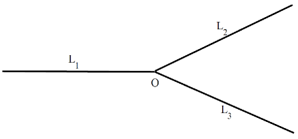
Figure 1: Sketch of a metric star graph. $L_{j}$ is the length of the $j$th bond with $j=1,2,3$.

II Vertex boundary conditions and exact solutions for star graph

The static sine-Gordon equation on a metric graph presented in Fig. 1 can be written as

$$\frac{d^{2}}{dx^{2}}\phi_{j}=\frac{1}{\lambda_{j}^{2}}\sin(\phi_{j}),\,0<x<L_{j},$$ (1)

where the wave functions $\phi_{j}$ are assigned to each bond of the graph and $j=1,2,3$ is the bond number. For wave equations on networks, the connections of the network wires at the vertices are provided by the vertex boundary conditions. In case of linear wave equations, the underlying constraint to derive vertex boundary conditions is the self-adjointness of the problem Kostrykin and Schrader (1999); Exner and Kovařík (2015). However, for nonlinear case one should use different conservation laws Sobirov et al. (2010); Adami et al. (2011); Caputo and Dutykh (2014). Here, for the stationary sine-Gordon equation we impose the boundary conditions providing flux conservation at the vertex

$$\lambda_{1}\left.\frac{d\phi_{1}}{dx}\right|_{x=0}=\lambda_{2}\left.\frac{d\phi_{2}}{dx}\right|_{x=0}=\lambda_{3}\left.\frac{d\phi_{3}}{dx}\right|_{x=0}$$ (2)

and the continuity of the weights of wave function derivatives, which are given as

$$\lambda_{1}\phi_{1}|_{x=0}+\lambda_{2}\phi_{2}|_{x=0}+\lambda_{3}\phi_{3}|_{x=0}=0.$$ (3)

The boundary conditions at the end of each bond are imposed as

$$\left.\frac{d\phi_{j}}{dx}\right|_{x=L_{j}}=2H_{j}.$$ (4)

The boundary conditions given by Eqs. (2)-(4) are consistent with other models of Josephson junction networks previously studied in Kogan et al. (2000); Susanto et al. (2005); Kuplevakhsky and Glukhov (2006, 2007). Exact solutions of Eq. (1) on a finite interval have been obtained earlier in Caputo et al. (2000); Susanto et al. (2005); Kuplevakhsky and Glukhov (2006, 2007) for different special cases. Here, we use an approach similar to that of the Refs. Kuplevakhsky and Glukhov (2006, 2007) to obtain exact analytical solutions of Eq. (1) for the boundary conditions (2) and (4).

II.1 Solution of type I

Our purpose is to obtain exact analytical solutions of the problem given by Eqs. (1)-(4). A solution of Eq. (1) without boundary conditions can be written as Kuplevakhsky and Glukhov (2006, 2007)

$$\phi_{j}^{(\pm)}(x)=(2n_{j}+1)\pi\pm 2\arcsin\left\{k_{j}\operatorname{sn}\left[\frac{x-x_{0,j}^{(\pm)}}{\lambda_{j}},k_{j}\right]\right\}$$ (5)

where $k_{j}$ and $x_{0,j}^{(\pm)}$ are integration constants and $\operatorname{sn}$ is Jacobi’s elliptic function. Depending on the value of $k_{j}$, the solution can be of two types. When $|H_{j}\lambda_{j}|\leq|k_{j}|\leq 1$, we refer to the solution as solution of type 1 Kuplevakhsky and Glukhov (2006). Taking into account that

$$\frac{d\phi_{j}^{(\pm)}}{dx}=\pm\frac{2k_{j}}{\lambda_{j}}\operatorname{cn}\left[\frac{x-x_{0,j}^{(\pm)}}{\lambda_{j}},k_{j}\right],$$ (6)

from boundary condition (4) we have

$$x_{0,j}^{(\pm)}=L_{j}-\lambda_{j}F\left[\arccos\left(\pm\frac{H_{j}\lambda_{j}}{k_{j}}\right),k_{j}\right].$$ (7)

Here, $\operatorname{cn}$ is Jacobi’s elliptic function Yanke and $F(\varphi,k)$ is the elliptic integral of the first kind Yanke. Then solution of type 1 of the sine-Gordon equation on a metric star graph with the boundary conditions (2)-(4) can be written as

$$\phi_{j}^{(\pm)}(x)=(2n_{j}+1)\pi\pm$$

$$\pm 2\arcsin\left\{k_{j}\operatorname{sn}\left[\frac{x-L_{j}}{\lambda_{j}}+F\left[\arccos\left(\pm\frac{H_{j}\lambda_{j}}{k_{j}}\right),k_{j}\right],k_{j}\right]\right\}$$

The vertex boundary conditions (2) and (3) lead to the following system of transcendental equations for finding $k_{j}$:

$$\underset{j=1}{\overset{3}{\sum}}\lambda_{j}\arcsin\left\{k_{j}\operatorname{sn}\left[\frac{L_{j}}{\lambda_{j}}-F\left[\arccos\left(\pm\frac{H_{j}\lambda_{j}}{k_{j}}\right),k_{j}\right],k_{j}\right]\right\}$$

$$=\pm\frac{1}{2}\underset{j=1}{\overset{3}{\sum}}(2n_{j}+1)\pi\lambda_{j},$$

(8)

$$k_{1}\operatorname{cn}\left[\frac{L_{1}}{\lambda_{1}}-F\left[\arccos\left(\pm\frac{H_{1}\lambda_{1}}{k_{1}}\right),k_{1}\right],k_{1}\right]=$$

$$=k_{2}\operatorname{cn}\left[\frac{L_{2}}{\lambda_{2}}-F\left[\arccos\left(\pm\frac{H_{2}\lambda_{2}}{k_{2}}\right),k_{2}\right],k_{2}\right],$$ (9)

$$k_{1}\operatorname{cn}\left[\frac{L_{1}}{\lambda_{1}}-F\left[\arccos\left(\pm\frac{H_{1}\lambda_{1}}{k_{1}}\right),k_{1}\right],k_{1}\right]=$$

$$=k_{3}\operatorname{cn}\left[\frac{L_{3}}{\lambda_{3}}-F\left[\arccos\left(\pm\frac{H_{3}\lambda_{3}}{k_{3}}\right),k_{3}\right],k_{3}\right].$$ (10)

It is clear that if this system has roots, then our problem has solutions. Here we obtain exact analytical solutions of this system for two special cases.
Case I is given by the relations

$$\lambda_{1}=\lambda_{2}+\lambda_{3},\,\frac{L_{j}}{\lambda_{j}}=2mK(k_{j}),\;m\in{\bf N},$$

$$H_{1}\lambda_{1}=H_{2}\lambda_{2}=H_{3}\lambda_{3}=H>0,$$

$$n_{1}=-n,\,n_{2}=n_{3}=n-1,\,n\in{\bf Z}.$$

From Eqs. (8)-(10) we have

$$k_{1}=k_{2}=k_{3}=k$$

and

$$g^{(\pm)}(k)\equiv(-1)^{m+1}k\sqrt{1-\left(\frac{H}{k}\right)^{2}}=0,$$

which gives

$$k=\pm H.$$

Case II corresponds to the constraints

$$\lambda_{1}=\lambda_{2}+\lambda_{3},\,\frac{L_{j}}{\lambda_{j}}=(-1)^{m_{j}}p+2m_{j}K(k_{j}),\,m_{j}\in{N}\cup\{0\},$$

$$H_{1}\lambda_{1}=H_{2}\lambda_{2}=H_{3}\lambda_{3}=H>0,$$

$$n_{1}=-n,\,n_{2}=n_{3}=n-1,\,n\in{\bf Z},$$

where $0<p<F\left[\arccos\left(H\right),1\right]$. Then from Eqs. (8)-(10) we have

$$k_{1}=k_{2}=k_{3}=k.$$

and

$$f^{(\pm)}(k)\equiv p-F\left[\arccos\left(\pm\frac{H}{k}\right),k\right]=0.$$ (11)

Since $f^{(\pm)}(\pm H)>0$, $f^{(\pm)}(\pm 1)<0$ and the functions $f^{(+)}(k)$ and ($f^{(-)}(k)$ are continuous on intervals $[H;1]$ and $[-1;-H]$), respectively, the system has at least one root. This can be seen from Fig. 2 where the function $f(k)$ is plotted.

Figure 2: Plot of the function $f(k)$ for $H=0.5\lambda_{1}=0.5,\lambda_{2}=0.2,\lambda_{3}=0.3,\;$ $m=1,p=1,n_{1}=-1,n_{2}=n_{3}=0,$ which shows the existence of a root of Eq. (11)

II.2 Solutions of type II

Solutions of type II for Eq. (1) are given by

$$\phi^{(\pm)}_{j}(x)=\pi(2n_{j}+1)\pm 2\operatorname{am}\left(\frac{x-x^{(\pm)}_{0,j}}{\lambda_{j}k_{j}},k_{j}\right),$$ (12)

and defined by the constraint

$$\frac{1}{\sqrt{1+H_{j}^{2}\lambda_{j}^{2}}}\leq|k_{j}|\leq\frac{1}{|H_{j}\lambda_{j}|}.$$

For the derivative of this solution, we have

$$\frac{d\phi_{j}^{(\pm)}(x)}{dx}=\pm\frac{2}{\lambda_{j}k_{j}}\operatorname{dn}\left(\frac{x-x^{(\pm)}_{0,j}}{\lambda_{j}k_{j}},k_{j}\right).$$ (13)

Inserting this derivative into the boundary condition (4) we obtain

$$x_{0,j}^{(\pm)}=L_{j}\mp\lambda_{j}k_{j}F\left(\arcsin\frac{\sqrt{1-H_{j}^{2}\lambda_{j}^{2}k_{j}^{2}}}{k_{j}},k_{j}\right).$$ (14)

Eqs. (12) - (14) together with the boundary conditions (2),(3) lead to

$$\underset{j=1}{\overset{3}{\sum}} \lambda_{j}\operatorname{am}\left[\frac{L_{j}}{\lambda_{j}k_{j}}\mp F\left(\arcsin\frac{\sqrt{1-H_{j}^{2}\lambda_{j}^{2}k_{j}^{2}}}{k_{j}},k_{j}\right),k_{j}\right]=$$

$$\displaystyle=\pm\frac{1}{2}\underset{j=1}{\overset{3}{\sum}}(2n_{j}+1)\pi\lambda_{j},$$

$$\frac{1}{k_{1}}\operatorname{dn}\left[\frac{L_{1}}{\lambda_{1}k_{1}}\mp F\left(\arcsin\frac{\sqrt{1-H_{1}^{2}\lambda_{1}^{2}k_{1}^{2}}}{k_{1}},k_{1}\right),k_{1}\right]=$$

$$=\frac{1}{k_{2}}\operatorname{dn}\left[\frac{L_{2}}{\lambda_{2}k_{2}}\mp F\left(\arcsin\frac{\sqrt{1-H_{2}^{2}\lambda_{2}^{2}k_{2}^{2}}}{k_{2}},k_{2}\right),k_{2}\right],$$

$$\frac{1}{k_{1}}\operatorname{dn}\left[\frac{L_{1}}{\lambda_{1}k_{1}}\mp F\left(\arcsin\frac{\sqrt{1-H_{1}^{2}\lambda_{1}^{2}k_{1}^{2}}}{k_{1}},k_{1}\right),k_{1}\right]=$$

$$\frac{1}{k_{3}}\operatorname{dn}\left[\frac{L_{3}}{\lambda_{3}k_{3}}\mp F\left(\arcsin\frac{\sqrt{1-H_{3}^{2}\lambda_{3}^{2}k_{3}^{2}}}{k_{3}},k_{3}\right),k_{3}\right].$$ (17)

Again, one can show the existence of solutions of Eqs. (II.2)-(17) for two special cases. For case I, which corresponds to the relations

$$\underset{j=1}{\overset{3}{\sum}}\left(2n_{j}\mp 2m+1\right)\lambda_{j}=0,\,m\in{\bf N}$$

$$\frac{L_{j}}{\lambda_{j}}=2mk_{j}K(k_{j}),\;m\in{\bf N},$$

$$H_{1}\lambda_{1}=H_{2}\lambda_{2}=H_{3}\lambda_{3}=H>1,$$ (18)

from Eqs. (II.2)-(17), we have

$$k_{1}=k_{2}=k_{3}=k,$$

$$g^{(\pm)}(k)\equiv\operatorname{am}\left[F\left(\arcsin\frac{\sqrt{1-H^{2}k^{2}}}{k},k\right),k\right]=0.$$ (19)

Then, Eq. (19) gives the following solution for the system of transcendental equations (II.2)-(17):

$$k=\pm\frac{1}{H}.$$

For case II, which is defined by the conditions

$$\frac{L_{j}}{\lambda_{j}}=k_{j}\left(p+2m_{j}K(k_{j})\right),\,m_{j}\in{N}\cup\{0\},$$

$$H_{1}\lambda_{1}=H_{2}\lambda_{2}=H_{3}\lambda_{3}=H>1,$$

$$\underset{j=1}{\overset{3}{\sum}}\left(2n_{j}\mp 2m_{j}+1\right)\lambda_{j}=0,$$

where $0<p<K\left(\frac{1}{\sqrt{1+H^{2}}}\right)$, Eqs. (II.2)-(17) yield

$$k_{1}=k_{2}=k_{3}=k,$$

that leads to

$$f^{(\pm)}(k)\equiv p\mp F\left[\arcsin\frac{\sqrt{1-H^{2}k^{2}}}{k},k\right]=0.$$ (20)

Since $f^{(\pm)}(\pm\frac{1}{H})>0$, $f^{(\pm)}(\pm\frac{1}{\sqrt{1+H^{2}}})<0$ and $f^{(+)}(k)$ $[\frac{1}{\sqrt{1+H^{2}}};\frac{1}{H}]$ ($f^{(-)}(k)$ is continuous on interval $[-\frac{1}{H};-\frac{1}{\sqrt{1+H^{2}}}]$), it has at least one root on this interval. Fig. 3 with the plot of $f(k)$ clearly shows that.

Figure 3: Plot of the function $f(k)$ for $H=2\lambda_{1}=0.5,\lambda_{2}=0.2,\lambda_{3}=0.3,\;$ $m_{1}=2,m_{2}=m_{3}=1,p=1,n_{1}=n_{2}=n_{3}=1,$ showing the existence of a root of Eq. (20)

.

III Applications of the method in tree graphs

The above discussion can also be applied to other simple topologies, such as tree graphs, loops and their combinations. Here, we briefly demonstrate this for the tree graph presented in Fig. 4.

The boundary conditions for each vertex and at the end of each bond can be written as

$$\left.\frac{d\phi_{1}}{dx}\right|_{x=0}=2H_{1},\,\left.\frac{d\phi_{1ij}}{dx}\right|_{x=L_{1ij}}=2H_{1ij},\,i=1,2,\,j=1,2,3,$$

$$\lambda_{1}\left.\frac{d\phi_{1}}{dx}\right|_{x=L_{1}}=\lambda_{1i}\left.\frac{d\phi_{1i}}{dx}\right|_{x=L_{i}},\,i=1,2,$$

$$\lambda_{1i}\left.\frac{d\phi_{1i}}{dx}\right|_{x=L_{1i}}=\lambda_{1ij}\left.\frac{d\phi_{1ij}}{dx}\right|_{x=L_{1i}},\,i=1,2,\,j=1,2,3,$$

$$\lambda_{1}\phi_{1}|_{x=L_{1}}+\lambda_{11}\phi_{11}|_{x=L_{1}}+\lambda_{12}\phi_{12}|_{x=L_{1}}=0,$$

$$\lambda_{1i}\phi_{1i}|_{x=L_{1i}}+\underset{j=1}{\overset{3}{\sum}}\lambda_{1ij}\phi_{1ij}|_{x=L_{1i}}=0,\,i=1,2.$$

Solutions of type 1 and 2 of Eq. (1) are defined similarly to those for star graphs and can be written as

$$\phi_{b}^{(\pm)}(x)=\left(2n_{b}+1\right)\pi\pm 2\arcsin\left\{k_{b}\operatorname{sn}\left[\frac{x-x_{0,b}^{(\pm)}}{\lambda_{b}},k_{b}\right]\right\},$$

$$\phi_{b}^{(\pm)}(x)=\left(2n_{b}+1\right)\pi\pm 2\operatorname{am}\left(\frac{x-x_{0,b}^{(\pm)}}{\lambda_{b}k_{b}},k_{b}\right).$$

Requiring these solutions to satisfy the boundary conditions leads to a system of transcendental equations for finding $k_{b}$. Again, exact solutions of this system can be obtained for two special cases. However, unlike the case of star graphs, for tree graphs, different bonds may have different type of solutions, e.g., one subgraph can have a solution of type 1, while for others it is possible to obtain the solution of type 2.

From the vertex boundary conditions we have the following system of transcendental equations:

$$\lambda_{1}\arcsin\left\{k_{1}\operatorname{sn}\left[\frac{L_{1}}{\lambda_{1}}-F\left[\arccos\left(\pm\frac{H_{1}\lambda_{1}}{k_{1}}\right),k_{1}\right],k_{1}\right]\right\}+$$

$$\lambda_{11}\arcsin\left\{k_{11}\operatorname{sn}\left[\frac{L_{1}-x_{0,11}^{(\pm)}}{\lambda_{11}},k_{11}\right]\right\}+$$

$$\lambda_{12}\arcsin\left\{k_{12}\operatorname{sn}\left[\frac{L_{1}-x_{0,12}^{(\pm)}}{\lambda_{12}},k_{12}\right]\right\}$$

$$=\mp\frac{\pi}{2}\left[(2n_{1}+1)\lambda_{1}+(2n_{11}+1)\lambda_{11}+(2n_{12}+1)\lambda_{12}\right],$$ (21)

$$\lambda_{1i}\arcsin\left\{k_{1i}\operatorname{sn}\left[\frac{L_{1i}-x_{0,1i}^{(\pm)}}{\lambda_{1i}},k_{1i}\right]\right\}+$$

$$+\overset{3}{\underset{j=1}{\sum}}\lambda_{1ij}\arcsin\left\{k_{1ij}\operatorname{sn}\left[\frac{L_{1i}-L_{1ij}}{\lambda_{1ij}}\right.\right.+$$

$$+\left.\left.F\left[\arccos\left(\pm\frac{H_{1ij}\lambda_{1ij}}{k_{1ij}}\right),k_{1ij}\right],k_{1ij}\right]\right\}$$

$$=\mp\frac{\pi}{2}\left[(2n_{1i}+1)\lambda_{1i}+\overset{3}{\underset{j=1}{\sum}}(2n_{1ij}+1)\lambda_{1ij}\right],$$ (22)

$$k_{1}\operatorname{cn}\left[\frac{L_{1}}{\lambda_{1}}-F\left[\arccos\left(\pm\frac{H_{1}\lambda_{1}}{k_{1}}\right),k_{1}\right],k_{1}\right]$$

$$=k_{1i}\operatorname{cn}\left[\frac{L_{1}-x_{0,1i}^{(\pm)}}{\lambda_{1i}},k_{1i}\right],$$ (23)

$$k_{1i}\operatorname{cn}\left[\frac{L_{1}-x_{0,1i}^{(\pm)}}{\lambda_{1i}},k_{1i}\right]$$

$$=k_{1}\operatorname{cn}\left[\frac{L_{1i}-L_{1ij}}{\lambda_{1ij}}+F\left[\arccos\left(\pm\frac{H_{1ij}\lambda_{1ij}}{k_{1ij}}\right),k_{1ij}\right],k_{1ij}\right],$$ (24)

where $i=1,2,\,j=1,2,3$. Choosing $x_{0,1i}^{(\pm)}=\frac{1}{2}(L_{1i}+L_{1})$ for case I we have

$$\lambda_{1}+\lambda_{11}+\lambda_{12}=0,\,\lambda_{1i}+\overset{3}{\underset{j=1}{\sum}}\lambda_{1ij}=0,$$

$$\frac{L_{1}}{\lambda_{1}}=2mK(k_{1}),\,\frac{L_{1ij}-L_{1i}}{\lambda_{1ij}}=2mK(k_{1ij}),$$

$$\frac{L_{1i}-L_{1}}{2\lambda_{1i}}=2mK(k_{1i})-F\left[\arccos\left(\pm\frac{H_{1}\lambda_{1}}{k_{1i}}\right),k_{1i}\right],$$

$$H_{1}\lambda_{1}=H_{1ij}\lambda_{1ij}=H>0,$$ (25)

where $i=1,2,\,j=1,2,3,\,m\in{\bf Z}\setminus\{0\}$. Then simplifying the above system of transcendental equations (21)-(24) will yield

$$k_{b}=k,\,g^{(\pm)}(k)\equiv(-1)^{m+1}k\sqrt{1-\left(\frac{H}{k}\right)^{2}}=0,$$

which together with Eq. (25) gives $k=\pm H$.

Figure 4: A metric tree graph.

For case II we have

$$\lambda_{1}+\lambda_{11}+\lambda_{12}=0,\,\lambda_{1i}+\overset{3}{\underset{j=1}{\sum}}\lambda_{1ij}=0,$$

$$\frac{L_{1}}{\lambda_{1}}=(-1)^{m_{1}}p+2m_{1}K(k_{1}),\,\frac{L_{1ij}-L_{1i}}{\lambda_{1ij}}=(-1)^{m_{1ij}}p+2m_{1ij}K(k_{1ij}),$$

$$\frac{L_{1i}-L_{1}}{2\lambda_{1i}}=(-1)^{m_{1i}}p+2m_{1i}K(k_{1i})-F\left[arccos\left(\pm\frac{H_{1}\lambda_{1}}{k_{1i}}\right),k_{1i}\right],$$

$$H_{1}\lambda_{1}=H_{1ij}\lambda_{1ij}=H>0,$$

where $0<p<F\left[arccos(H),1\right]$ and $i=1,2,\,j=1,2,3,\,m\in{\bf Z}$. For this case the solution of Eqs. (21)-(24) can be written as

$$k_{b}=k,\,f^{(\pm)}(k)\equiv p-F\left[arccos\left(\pm\frac{H}{k}\right),k\right].$$

Since $f^{(\pm)}(\pm\frac{1}{H})>0$, $f^{(\pm)}(\pm 1)<0$ and the function $f^{(+)}(k)$ $[\frac{1}{H};1]$ ($f^{(-)}(k)$ is continuous on interval $[-1;-\frac{1}{H}]$), it has at least one root on this interval. We note that similarly, one can obtain solutions of mixed types.

IV Stability of solutions

Here we briefly analyze the stability of the obtained solutions using the same method as in the Refs.Kuplevakhsky and Glukhov (2006, 2007). We do this for a metric star graph, however, extending the method to tree graphs and other graph topologies is trivial. First we define the Gibbs free-energy functional on the star graph presented in Fig. 1

$$\Omega_{G}=\underset{j=1}{\overset{3}{\sum}}\Omega_{G}^{(j)}\left[\phi_{j},\,\frac{d\phi_{j}}{dx};\,H_{j}\right],$$ (26)

with the Gibbs free energy on each bond given by

$$\Omega_{G}^{(j)}\left[\phi_{j},\,\frac{d\phi_{j}}{dx};\,H_{j}\right]=2H_{j}^{2}W_{j}-2H_{j}\left[\phi_{j}(L_{j})-\phi_{j}(0)\right]$$

$$+\frac{1}{\lambda_{j}}\underset{0}{\overset{L_{j}}{\int}}\left[1-cos\phi_{j}(x)+\frac{\lambda_{j}^{2}}{2}\left[\frac{d\phi_{j}(x)}{dx}\right]^{2}\right]dx.$$ (27)

$W_{j}$ is the length of the bond $j$. It is easy to see that the condition $\delta\Omega_{G}=0$ leads to the sine-Gordon equation on a star graph given by Eqs. (1)-(4).

The key role in the stability analysis is played by the second variation of the Gibbs functional given by

$$\delta^{2}\Omega_{G}=\underset{j=1}{\overset{3}{\sum}}\frac{1}{\lambda_{j}}\underset{0}{\overset{L_{j}}{\int}}\left[cos\bar{\phi_{j}}(\delta\phi_{j})^{2}+\lambda_{j}^{2}\left(\frac{d\delta\phi_{j}}{dx}\right)^{2}\right]dx.$$

If for the tested solution of the sine-Gordon equation, $\phi_{j}(x)=\bar{\phi}_{j}(x)$

$$\delta^{2}\Omega_{G}\left[\phi_{j},\frac{d\phi_{j}}{dx}\right]_{\phi_{j}(x)=\bar{\phi}_{j}(x)}>0,$$

the solution will be inside the stability region Kuplevakhsky and Glukhov (2006, 2007). For $\delta^{2}\Omega_{G}\left[\phi_{j},\frac{d\phi_{j}}{dx}\right]_{\phi_{j}(x)=\bar{\phi}_{j}(x)}$ having no definite sign, the solution will be unstable Kuplevakhsky and Glukhov (2006, 2007). The condition

$$\delta^{2}\Omega_{G}\left[\phi_{j},\,\frac{d\phi_{j}}{dx}\right]_{\phi_{j}(x)=\bar{\phi}_{j}(x)}\geq 0,$$

defines the border of stability (bifurcation point). Furthermore, following Refs. Kuplevakhsky and Glukhov (2006, 2007), these three conditions can be reformulated in terms of $\mu_{0}$, the lowest eigenvalue of the Sturm-Liouville eigenvalue problem

$$-\lambda_{j}^{2}\frac{d^{2}\psi_{j}}{dx^{2}}+cos\bar{\phi_{j}}\psi_{j}=\mu\psi_{j},$$ (28)

$$\lambda_{1}\left.\frac{d\psi_{1}}{dx}\right|_{x=0}=\lambda_{2}\left.\frac{d\psi_{2}}{dx}\right|_{x=0}=\lambda_{3}\left.\frac{d\psi_{3}}{dx}\right|_{x=0}$$ (29)

$$\lambda_{1}\psi_{1}|_{x=0}+\lambda_{2}\psi_{2}|_{x=0}+\lambda_{3}\psi_{3}|_{x=0}=0,$$ (30)

$$\left.\frac{d\psi_{j}}{dx}\right|_{x=L_{j}}=0,\,j=1,2,3.$$ (31)

If the lowest eigenvalue $\mu=\mu_{0}$ of this Sturm-Liouville problem is negative, i.e. $\mu_{0}<0$, the solution $\phi=\phi(y)$ corresponds to a saddle point of Eq. (27) and therefore is unstable. The stable solutions minimize the functional $\Omega_{G}$ and are characterized by $\mu_{0}>0$. The boundary between stable and unstable solutions are determined by the condition $\mu=0$. By solving numerically the problem (28) -(31) we found that $\mu_{0}<0$ for both cases of the solutions of type 1. For the case I of the solution of type 2 we have $\mu_{0}>0$, while for the case II of the solution of type 2 we found that $\mu_{0}<0$. Therefore only case I of the solution of type 2 is stable, while the other solutions are unstable.

V Conclusions

In this paper, we have studied the stationary sine-Gordon equation on simple metric graphs by imposing the vertex boundary conditions following from the flux conservation and the continuity of the weights of the wave function derivatives. Exact analytical solutions are obtained for a metric star graph. The constraints allowing such exact solutions are determined in terms of bond nonlinearity coefficients.

The treatment has been extended to metric tree graphs and explicit solutions are derived. Generalizations to other simple topologies such as loop graphs and combinations of loop and star graphs have also been discussed. The stability of the obtained solutions has been analyzed. The obtained results can be directly applied to the study of static solitons in 2D branched Josephson junctions in a constant magnetic field, i.e. T-, Y- and tree-shaped versions of the model studied in Kuplevakhsky and Glukhov (2006). Finally, we note that the method can be extended to the case of ”current carrying” boundary conditions studied in Ref. Kuplevakhsky and Glukhov (2007).

VI Acknowledgements

We thank Dmitry Pelinovsky for his useful comments on the paper. This work is supported by a grant of the Volkswagen Foundation. The work of KS is partially supported by the grant of the Committee for the Coordination Science and Technology Development (Ref.Nr. F-2-003).