Reduced Order Models for Pricing European and American Options under Stochastic Volatility and Jump-Diffusion Models

Abstract

European options can be priced by solving parabolic partial(-integro) differential equations under stochastic volatility and jump-diffusion models like Heston, Merton, and Bates models. American option prices can be obtained by solving linear complementary problems (LCPs) with the same operators. A finite difference discretization leads to a so-called full order model (FOM). Reduced order models (ROMs) are derived employing proper orthogonal decomposition (POD). The early exercise constraint of American options is enforced by a penalty on subset of grid points. The presented numerical experiments demonstrate that pricing with ROMs can be orders of magnitude faster within a given model parameter variation range.

1 Introduction

European options can be exercised only at expiry while American options can be exercised anytime until expiry. Due to this additional flexibility the American options can be more valuable. In order to avoid arbitrage the price must be always at least the same as the final payoff function. A put option gives the right to sell the underlying asset for a specified strike price while a call option gives the right to buy the asset for a strike price. The seminal paper [1] by Black and Scholes employs a geometrical Brownian motion with a constant volatility as a model for the price of the underlying asset. The market prices of options show that the volatility varies depending on the strike price and expiry of option. Several more generic models for the asset prices have been developed which are more consistent with market prices. Merton proposed adding log-normally distributed jumps to this model [2]. Heston [3] made the volatility to be a mean reverting stochastic process. Bates [4] combined the Heston stochastic volatility model and Merton jump-diffusion model.

There are many methods for pricing options. The Monte Carlo method simulate asset price paths to compute the option price. This is an intuitive and flexible method, but it can be slow when high precision is require and it is more complicated and less efficient for American options. Instead in this paper, the pricing is based on partial(-integro) differential equation (P(I)DE) formulations. Another approach is based on numerical integration techniques. One benefit of these formulations is that for many options they can provide a highly accurate price much faster than the Monte Carlo method. Here the European options are priced by solving a P(I)DE and the American options by solving an LCP with the same operator. These operators are two-dimensional with a stochastic volatility and one-dimensional otherwise. The potential integral part of the model results from the jumps.

The most common way to discretize the differential operators is the finite difference method. For European and American options the discrization leads to a system of linear equations and an LCP, respectively, at each time step. Under stochastic volatility models efficient PDE based methods for American options have been considered in [5, 6, 7, 8], for example. A penalty approximation is employed for the resulting LCPs in [8] and an operator splitting method in [6, 7]. An alternating direction implicit (ADI) method is used in [6] while iterative methods are used for resulting linear systems in [5, 7, 8]. Under jump-diffusion models PIDE methods lead to a system with a full matrix at each time step and their efficient solution for American options has been considered in [9, 10, 11, 12, 13], for example. A penalty method together with FFT based fast method for evaluating the jump integral was used in [9]. An iterative method was proposed for LCPs with full matrices in [11]. An implicit-explicit (IMEX) method was proposed in [10] to treat the integral term explicitly and the same approach was studied in [13]. The generalizations of the above methods for the combined Bates model have been developed and studied in [14, 15, 16, 17, 18].

Unfortunately, such high-fidelity simulations are still too expensive for many practical applications and reduced order modeling (ROM) is a promising tool for significantly alleviating computational costs [19, 20]. Most existing ROM approaches are based on projection. In projection-based reduced order modeling the state variables are approximated in a low-dimensional subspace. Bases for this subspace are typically constructed by Proper Orthogonal Decomposition (POD) [21] of a set of high-fidelity solution snapshots. While many approaches have already been developed for the efficient reduction of linear computational models three main strategies have been explored so far for efficiently reducing nonlinear computational models. The first one is based on linearization techniques [22, 23]. The second one is based on the notion of precomputations [24, 25, 26, 27, 28], but is limited to polynomial nonlinearities. The third strategy relies on the concept of hyper-reduction — that is, the approximation of the reduced operators underlying a nonlinear reduced-order model (ROM) by a scalable numerical technique based on a reduced computational domain [29, 30, 31, 32, 33, 34, 35, 36].

In the case where the governing equations include a constraint equation it is often beneficial to construct a basis that satisfies these constraints a priori [37]. For example, in the case of non-negativity constraints, a non-negative basis can be constructed via non-negative matrix factorization (NNMF) [38]. This approach was employed for option pricing in [39].

For pricing European options ROMs have been developed in [40, 41]. Only recently ROMs have been applied for pricing American options in [37, 42]. A common problem associated with option pricing is the calibration of model parameters to correspond to the market prices of options. This is typically formulated as a least squares -type optimization problem. The calibration is computationally expensive as it requires pricing a large number of options with varying parameters. The use of ROMs to reduce this computational cost has been studied in [43, 44, 45].

The main contribution of the present work is the development of a cheap and accurate hyper-reduction approach for the early exercise constraint of American options. Our proposed approach is based on the fact that accurate price predictions do not necessarily require accurate approximations of the Lagrange multipliers. This has been observed in practice for the reduction of structural contact problems [38]. Our numerical experiments summarized in this paper suggest that using the binary matrix as the basis for the Lagrange multipliers performs remarkably well for all reproductive and predictive simulations considered. This approach is simpler, faster, and comparable in accuracy to previous approaches based on the NNMF [39].

This paper is organized as follows. In Section 2, the full order models considered in this work are overviewed. In Section 3 the proposed new ROM approach is laid out. In Section 4 the proposed approach is applied to several problems. Finally in Section 5, conclusions are offered and prospects for future work are summarized.

2 Full Order Models

Merton [2] proposed the price $s\geq 0$ of an underlying asset to follow the stochastic differential equation

$$ds=(g-\mu\xi)sdt+\sigma_{s}sdw_{s}+sdJ,$$ (1)

where $t$ is the time, $g$ is the growth rate of the asset price, $\sigma_{s}$ is its volatility, $w_{s}$ is a Wiener process, and $J$ is a compound Poisson process with the jump intensity $\mu$ and the log-normal jump distribution

$$p(y)=\frac{1}{y\delta\sqrt{2\pi}}\exp\left(-\frac{(\log y-\gamma)^{2}}{2\delta^{2}}\right).$$ (2)

The relative expected jump is $\xi=\exp\left(\gamma+\tfrac{1}{2}\delta^{2}\right)-1$. The Black–Scholes model is obtained by setting the jump intensity $\mu$ to zero. Under the Merton model the price $u(s,\tau)$ of a European option can be obtained by solving the one-dimensional PIDE

$$\frac{\partial u}{\partial\tau}=\frac{1}{2}\sigma_{s}^{2}s^{2}\frac{\partial^{2}u}{\partial s^{2}}+(r-\mu\xi)s\frac{\partial u}{\partial s}-(r+\mu)u+\mu\int_{0}^{\infty}u(sy,\tau)p(y)dy=:L^{M}u,$$ (3)

where $\tau=T-t$ is the time until expiry, $T$ is the expiry time, $r$ is the interest rate.

Bates [4] proposed the price $s$ and its instantaneous variance $v\geq 0$ to follow the stochastic differential equations

$$\begin{split}ds&=(g-\mu\xi)sdt+\sqrt{v}sdw_{s}+sdJ\\ dv&=\kappa(\theta-v)dt+\sigma_{v}\sqrt{v}dw_{v},\\ \end{split}$$ (4)

where $\theta$ is the mean level of $v$, $\kappa$ is the rate of mean reversion, $\sigma_{v}$ is the volatility of $\sqrt{v}$, and $w_{v}$ is a Wiener process. The Wiener prosesses $w_{s}$ and $w_{v}$ have the correlation $\rho$. Under the Bates model the price $u(s,v,\tau)$ of a European option can be obtained by solving the two-dimensional PIDE

$$\begin{split}\frac{\partial u}{\partial\tau}&{}=\frac{1}{2}vs^{2}\frac{\partial^{2}u}{\partial s^{2}}+\rho\sigma_{v}vs\frac{\partial^{2}u}{\partial s\partial v}+\frac{1}{2}\sigma_{v}^{2}v\frac{\partial^{2}u}{\partial v^{2}}+(r-\mu\xi)s\frac{\partial u}{\partial s}+\kappa(\theta-v)\frac{\partial u}{\partial v}\\ &{}-(r+\mu)u+\mu\int_{0}^{\infty}u(sy,v,\tau)p(y)dy=:L^{B}u,\end{split}$$ (5)

The Heston model is obtained by setting the jump intensity $\mu$ to zero.

In the following, put options are considered. Their price at the expiry is given by the pay-off function $g(s)=\max\{K-s,\,0\}$. As the equations are solved backward in time, this leads to the initial condition

$$u(s,0)=g(s)\qquad\text{and}\qquad u(s,v,0)=g(s)$$ (6)

for one-dimensional and two-dimensional models, respectively.

For computing an approximate solution the infinite domain is truncated at $s=s_{\max}$ and $v=v_{\max}$, where $s_{\max}$ and $v_{\max}$ are sufficiently large so that the error due to truncation is negligible. The price $u$ of a European put option satisfies the Dirichlet boundary conditions

$$u=Ke^{-r\tau}\;\;\text{at}\;\;s=0\qquad\text{and}\qquad u=0\;\;\text{at}\;\;s=s_{\max}.$$ (7)

For a non-negative interest rate $r\geq 0$, the price $u$ of an American put option satisfies the Dirichlet boundary conditions

$$u=K\;\;\text{at}\;\;s=0\qquad\text{and}\qquad u=0\;\;\text{at}\;\;s=s_{\max}.$$ (8)

Under the stochastic volatility models, the Neumann boundary condition $\tfrac{\partial u}{\partial v}=0$ is posed at $v=v_{\max}$. The second derivatives in (5) vanish on the boundary $v=0$. It is shown in [46] that this degenerated form defines appropriate boundary condition at $v=0$.

Due to early exercise possibility the price $u$ of an American option satisfies the LCP

$$\tfrac{\partial u}{\partial\tau}-Lu=\lambda,\quad u\geq g,\quad\lambda\geq 0,\quad\lambda(u-g)=0,$$ (9)

where the operator $L$ is either $L^{M}$ or $L^{B}$ depending on the model and $\lambda$ is a Lagrange multiplier; see [47], for example.

For an easier numerical solution, the P(I)DE for European options and the LCP for American options are reformulated for $w$ which satisfies the homogeneous Dirichlet boundary condition $w=0$ at $s=0$. Furthermore, $w$ for American options is chosen so that it satisfies the positivity constraint $w\geq 0$ instead of the more complicated constraint $u\geq g$. For European options $w$ is chosen to be $w=u-e^{-r\tau}g$ while for American options it is chosen to be $w=u-g$.

For European options the choice $w=u-e^{-r\tau}g$ leads to the P(I)DE

$$\tfrac{\partial w}{\partial\tau}-Lw=e^{-r\tau}(L+r)g.$$ (10)

For American options the choice $w=u-g$ leads to the LCP

$$\tfrac{\partial w}{\partial\tau}-Lw=\lambda+Lg,\quad w\geq 0,\quad\lambda\geq 0,\quad\lambda w=0.$$ (11)

For American options a quadratic penalty formulation is obtained by choosing the Lagrange multiplier to be

$$\lambda=-\tfrac{1}{\varepsilon}\max\left\{-w,0\right\}w.$$ (12)

This leads to the nonlinear P(I)DE

$$\tfrac{\partial w}{\partial\tau}-Lw+\tfrac{1}{\varepsilon}\max\left\{-w,\,0\right\}w=Lg.$$ (13)

For the finite difference discretization, a grid is defined by $s_{i}$, $i=0,1,2,\ldots,N_{s}$, for the interval $[0,s_{\max}]$. The spatial partial derivatives with respect to $s$ are discretized using central finite difference

$$\frac{\partial w}{\partial s}(s_{i})\approx\tfrac{1}{\Delta s_{i-1}+\Delta s_{i}}\left[-\tfrac{\Delta s_{i}}{\Delta s_{i-1}}w_{i-1}+\left(\tfrac{\Delta s_{i}}{\Delta s_{i-1}}-\tfrac{\Delta s_{i-1}}{\Delta s_{i}}\right)w_{i}+\tfrac{\Delta s_{i-1}}{\Delta s_{i}}w_{i+1}\right]$$ (14)

and

$$\frac{\partial^{2}w}{\partial s^{2}}(s_{i})\approx\tfrac{2}{\Delta s_{i-1}+\Delta s_{i}}\left[\tfrac{1}{\Delta s_{i-1}}w_{i-1}-\left(\tfrac{1}{\Delta s_{i-1}}+\tfrac{1}{\Delta s_{i}}\right)w_{i}+\tfrac{1}{\Delta s_{i}}w_{i+1}\right],$$ (15)

where $\Delta s_{i}=s_{i+1}-s_{i}$. Similarly for the interval $[0,v_{\max}]$, a grid is defined $v_{j}$, $j=0,1,2,\ldots,N_{v}$. The spatial partial derivatives with respect to $v$ are discretized using the above central finite differences. A nine-point finite difference stencil for $\tfrac{\partial^{2}w}{\partial s\partial v}$ is obtained by employing the central finite differences in both directions. While this approximation can be unstable with high correlations $\rho$ it is stable for numerical experiments presented in Section 4. On the boundary $v=0$, a one-sided finite difference approximation is used for $\tfrac{\partial w}{\partial v}$. The integrals can be discretized using a second-order accurate quadrature formula. Here the linear interpolation is used for $w$ between grid points and exact integration; see [11], for details. Under the Merton model the discretization of the integral leads to a full matrix while under the Bates model it leads to full diagonal blocks.

Under models without jumps the time discretization is performed by taking the first time steps using the implicit Euler method and after using the second-order accurate BDF2 method. Under jump models the integral is treated explicitly. In the first time step using the explicit Euler method and in the following time steps using the linear extrapolation based on the two previous time steps. This IMEX-BDF2 method is described in [13]. With the explicit treatment of the integral it is not necessary to solve systems with dense matrices. At the time $(k+1)\Delta\tau$, the grid point values contained in the vector ${\bf w}^{k+1}$ are obtained by solving the system

$$\left({\bf I}+\tfrac{2}{3}\Delta\tau{\bf D}\right){\bf w}^{k+1}\\ =\left(\tfrac{4}{3}{\bf w}^{k}-\tfrac{1}{3}{\bf w}^{k-1}\right)+\Delta\tau{\bf J}\left(\tfrac{4}{3}{\bf w}^{k}-\tfrac{2}{3}{\bf w}^{k-1}\right)+\tfrac{2}{3}\Delta\tau{\bf f}$$ (16)

for European options and

$$\begin{split}&\left({\bf I}+\tfrac{2}{3}\Delta\tau{\bf D}+\tfrac{1}{\varepsilon}\operatorname*{diag}\left(\max\left\{-{\bf w}^{k+1},\,0\right\}\right)\right){\bf w}^{k+1}\\ &{}=\left(\tfrac{4}{3}{\bf w}^{k}-\tfrac{1}{3}{\bf w}^{k-1}\right)+\Delta\tau{\bf J}\left(\tfrac{4}{3}{\bf w}^{k}-\tfrac{2}{3}{\bf w}^{k-1}\right)+\tfrac{2}{3}\Delta\tau{\bf f}\end{split}$$ (17)

for American options, where the matrices ${\bf J}$ and ${\bf D}$ corresponds to the terms due to the jumps and the rest, respectively. The vector ${\bf f}$ contains the grid point values of $e^{-r\tau}(L+r)g$ and $Lg$. The operator $\operatorname*{diag}(\cdot)$ gives a diagonal matrix with the diagonal entries defined by the argument vector. The maximum is taken componentwise. The systems (16) and (17) can be expressed more compactly as

$${\bf A}{\bf w}^{k+1}={\bf r}^{k+1}$$ (18)

and

$$\left({\bf A}+\tfrac{1}{\varepsilon}\operatorname*{diag}\left(\max\left\{-{\bf w}^{k+1},\,0\right\}\right)\right){\bf w}^{k+1}={\bf r}^{k+1}$$ (19)

with suitably defined ${\bf A}$ and ${\bf r}^{k+1}$. The discrete counterpart of the Lagrange multiplier $\lambda$ in (12) reads

$${\boldsymbol{\lambda}}^{k+1}=-\tfrac{1}{\varepsilon}\operatorname*{diag}\left(\max\left\{-{\bf w}^{k+1},\,0\right\}\right){\bf w}^{k+1}.$$ (20)

3 Reduced Order Models

Let ${\bf U}\in{\mathbb{R}}^{N\times n}$ be the basis for ${\bf w}$ with $n\ll N$. These basis are constructed by applying POD to a collection of solution snapshots. A solution snapshot, or simply a snapshot, is defined as a state vector ${\bf w}^{k}$ computed as the solution of (17) for some instance of its parameters. A solution matrix is defined as a matrix whose columns are individual snapshots.

To construct ${\bf U}$, the following optimization problem is solved

$$\underset{{\bf U}\in\mathbb{R}^{N\times n},\,{\bf V}\in\mathbb{R}^{n\times K}}{\text{minimize}}\displaystyle\|{\bf X}-{\bf U}{\bf V}\|_{F}^{2},$$ (21)

where $K$ is the number of solution snapshots. Hence, the basis ${\bf U}$ is comprised of the first $n$ left singular vectors of the snapshot matrix ${\bf X}$ and ${\bf V}=\SS{\bf W}^{T}$, where $\SS$ is the diagonal matrix of the first $n$ singular values of $\SS$, and ${\bf W}$ is the matrix of its first $n$ right singular vectors.

For European options the reduced solution ${\bf w}={\bf U}{\bf w}_{r}$ is governed by

$${\bf U}^{T}{\bf A}{\bf U}{\bf w}_{r}^{k+1}={\bf U}^{T}{\bf r}^{k+1}.$$ (22)

This ROM has the form

$${\bf A}_{r}{\bf w}_{r}^{k+1}={\bf r}_{r}^{k+1},$$ (23)

where ${\bf A}_{r}={\bf U}^{T}{\bf A}{\bf U}$ is precomputed offline while the right-hand side ${\bf r}_{r}^{k+1}={\bf U}^{T}{\bf r}$ can be computed efficiently online with the number of operations depending on $n$. Thus, the online computational cost of forming and solving the problems (23) scales with the size $n$ of the reduced basis and it does not depend on the size $N$ of FOM.

For American options the reduced solution ${\bf w}={\bf U}{\bf w}_{r}$ is governed by

$$\left({\bf U}^{T}{\bf A}{\bf U}+\tfrac{1}{\varepsilon}{\bf U}^{T}\operatorname*{diag}\left(\max\left\{-{\bf U}{\bf w}_{r}^{k+1},\,0\right\}\right){\bf U}\right){\bf w}_{r}^{k+1}\\ ={\bf U}^{T}{\bf r}^{k+1}.$$ (24)

The product ${\bf U}^{T}\operatorname*{diag}\left(\max\left\{-{\bf U}{\bf w}_{r}^{k+1},\,0\right\}\right){\bf U}$ is the only product in (24) that cannot be precomputed offline. Since the cost of evaluating this product scales with the size of the full order model, Eq. (24) does not offer major computational savings.

To attain computational savings, the traditional approach involves including a second layer of approximation, sometimes called “hyper-reduction”. One of the most popular hyper-reduction approaches is the Discrete Empirical Interpolation Method (DEIM) [31]. We recapitulate the traditional DEIM algorithm as a starting point for our innovation.

Let ${\bf U}_{\lambda}\in{\mathbb{R}}^{N\times n_{\lambda}}$ be basis for $\max\left\{-{\bf U}{\bf w}_{r}^{k+1},\,0\right\}$, thus

$${\bf U}_{\lambda}{\bf h}_{r}\approx\max\left\{-{\bf U}{\bf w}_{r}^{k+1},\,0\right\},$$ (25)

where ${\bf h}_{r}$ is the corresponding coefficient vector. The vector ${\bf h}_{r}$ can be determined by selecting $m$ unique rows from the overdetermined system ${\bf U}_{\lambda}{\bf h}_{r}\approx\max\left\{-{\bf U}{\bf w}_{r}^{k+1},\,0\right\}$. Specifically, consider a binary matrix ${\bf P}\in\{0,1\}^{N\times n_{\lambda}}$ satisfying ${\bf P}^{T}{\bf P}={\bf I}_{n_{\lambda}}$. Assuming ${\bf P}^{T}{\bf U}$ is nonsingular, the coefficient vector ${\bf h}_{r}$ can be determined uniquely from

$${\bf P}^{T}\max\left\{-{\bf U}{\bf w}_{r}^{k+1},\,0\right\}=({\bf P}^{T}{\bf U}_{\lambda}){\bf h}_{r}$$ (26)

and the final approximation is

$$\max\left\{-{\bf U}{\bf w}_{r}^{k+1},\,0\right\}\approx{\bf U}_{\lambda}{\bf h}_{r} ={\bf U}_{\lambda}({\bf P}^{T}{\bf U}_{\lambda})^{-1}{\bf P}^{T}\max\left\{-{\bf U}{\bf w}_{r}^{k+1},\,0\right\}$$ (27)

$$=\widetilde{{\bf U}}_{\lambda}\max\left\{-{\bf C}{\bf w}_{r}^{k+1},\,0\right\},$$ (28)

where $\widetilde{{\bf U}}_{\lambda}={\bf U}_{\lambda}({\bf P}^{T}{\bf U}_{\lambda})^{-1}$, and ${\bf C}={\bf P}^{T}{\bf U}$.

Thus, the product ${\bf U}^{T}\operatorname*{diag}\left(\max\left\{-{\bf U}{\bf w}_{r}^{k+1},\,0\right\}\right){\bf U}$ in Eq. (24) is approximated by ${\bf U}^{T}\operatorname*{diag}\left(\widetilde{{\bf U}}_{\lambda}\max\left\{-{\bf C}{\bf w}_{r}^{k+1},\,0\right\}\right){\bf U}$ that, unlike its predecessor, can be computed efficiently online. In particular

$${\bf U}^{T}\operatorname*{diag}\left(\widetilde{{\bf U}}_{\lambda}\max\left\{-{\bf C}{\bf w}_{r}^{k+1},\,0\right\}\right){\bf U}=\sum_{i=1}^{n_{\lambda}}{\bf K}_{i}\max\left\{-\left[{\bf C}{\bf w}_{r}^{k+1}\right]_{i},\,0\right\},$$ (29)

where ${\bf K}_{i}={\bf U}^{T}\operatorname*{diag}\left(\left[\widetilde{{\bf U}}_{\lambda}\right]_{:,i}\right){\bf U}$ and $\left[\widetilde{{\bf U}}_{\lambda}\right]_{:,i}$ refers to the $i^{\text{th}}$-column of $\widetilde{{\bf U}}_{\lambda}$. The matrices ${\bf K}_{i}$ can be computed offline, once and for all, while $\max\left\{-\left[{\bf C}{\bf w}_{r}^{k+1}\right]_{i},\,0\right\}$ can be computed efficiently online since ${\bf C}\in\mathbb{R}^{n_{\lambda}\times n}$ does not scale with the size of the full order model.

Although this straightforward implementation of DEIM succeeds in reducing the computational complexity of the ROM, this approach cannot be expected to yield accurate price predictions because DEIM does not enforce non-negativity. Even if the basis ${\bf U}_{\lambda}$ are constructed to be non-negative a priori, using, for example, NNMF, non-negativity is still not guaranteed because $\widetilde{{\bf U}}_{\lambda}={\bf U}_{\lambda}({\bf P}^{T}{\bf U}_{\lambda})^{-1}$ is not guaranteed to be non-negative. One possible remedy is use instead a non-negative variation of the DEIM, called NNDEIM [48]. Yet another remedy involves an angle-greedy procedure for constructing the non-negative bases [37]. In this work, we introduce an alternative approach that does not require computation of non-negative basis for the Lagrange multipliers.

Our proposed approach is based on the fact that accurate price predictions do not necessarily require accurate approximations of the Lagrange multipliers. In particular, requiring that ${\bf U}_{\lambda}{\bf h}_{r}\approx\max\left\{-{\bf U}{\bf w}_{r}^{k+1},0\right\}$ may not be necessary. This has been observed in practice for the reduction of structural contact problems [38]. Our numerical experiments summarized in this paper suggest that using the binary matrix ${\bf P}$ as the basis for the Lagrange multipliers performs remarkably well for all reproductive and predictive simulations considered. With this approximation, the reduced order model simplifies considerably. In particular, with ${\bf U}_{\lambda}={\bf P}$, $\widetilde{{\bf U}}_{\lambda}={\bf P}$ and thus, the product ${\bf U}^{T}\operatorname*{diag}\left(\max\left\{-{\bf U}{\bf w}_{r}^{k+1},\,0\right\}\right){\bf U}$ in Eq. (24) is approximated by the relatively simple product ${\bf C}^{T}\operatorname*{diag}\left(\max\left\{-{\bf C}{\bf w}_{r}^{k+1},\,0\right\}\right){\bf C}$. Thus, the final form of the ROM is as follows

$$\left({\bf A}_{r}+\tfrac{1}{\varepsilon}{\bf C}^{T}\operatorname*{diag}\left(\max\left\{-{\bf C}{\bf w}_{r}^{k+1},\,0\right\}\right){\bf C}\right){\bf w}_{r}^{k+1}\\ ={\bf r}^{k+1}_{r},$$ (30)

where ${\bf A}_{r}={\bf U}^{T}{\bf A}{\bf U}$, and ${\bf r}_{r}={\bf U}^{T}{\bf r}$. All components in Equation (30) scale with the size of the reduced order model.

Finally, to construct the selection matrix ${\bf P}$, the standard DEIM algorithm for selecting the interpolation indices is utilized [31]. However, in our proposed approach, the DEIM algorithm is applied to ${\bf m}\odot{\bf U}_{:,i}$, for $i=1,2,\ldots,n$, where ${\bf m}\in\{0,1\}^{N\times 1}$ is a binary mask vector. The non-zero elements of the mask vector ${\bf m}$, correspond to elements in the snapshots where early exercise has occurred at least once, that is, elements $j$ such that ${\bf U}_{j,i}\leq 0$ for any $i$. The binary mask vector ensures consistency with the nonlinear function that is being approximated, i.e. $\max\left\{-{\bf U}{\bf w}_{r}^{k+1},\,0\right\}$.

4 Numerical Experiments

All numerical examples considered here price a European put option and an American put option with the strike price $K=100$ and the expiry $T=0.5$. Only at the money options are considered, that is, the value of $u$ at $s=K$ is sought. Under the stochastic volatility models the value of $u$ is computed at the instantaneous variance $v=\theta$. The full order models are discretized using quadratically refined spatial grids similar to ones employed by the FD-NU method in [49]. The $s$-grid is defined by $s_{i}=\left[\left(\tfrac{i}{\alpha N_{s}}-1\right)\left|\tfrac{i}{\alpha N_{s}}-1\right|+1\right]K$, $i=0,1,\ldots,N_{s}$ with $\alpha=\tfrac{3}{8}$. For the stochastic volatility models the variance grid is defined by $v_{j}=\left(\tfrac{j}{N_{v}}\right)^{2}v_{\max}$ with $v_{\max}=1$. The uniform time steps are given by $\Delta\tau=\tfrac{1}{N_{\tau}}T$. In the experiments the number of spatial and temporal steps are chosen to be $N_{s}=128$, $N_{v}=64$, and $N_{\tau}=32$. With this choice and the employed parameter ranges the absolute discretization error is about $10^{-2}$ or less. In the case of the American option, an iteration reduces the penalty parameter $\varepsilon$ with the five values $10^{-1}$, $10^{-2}$, $10^{-3}$, $10^{-4}$, and $10^{-5}$. This is the main reason for higher run times with the American option.

The snapshot matrix ${\bf X}$ is given by all vectors ${\bf w}^{k}$, $k=1,2,\ldots,N_{\tau}$, in all training runs. For these training runs each model parameter is sampled at its extreme values and at the midpoint between them. Thus, with two, five, and eight model parameters there are $3^{2}=9$, $3^{5}=243$, and $3^{8}=6561$ training runs, respectively. In the predictive ROM simulations, each parameter has two values which are the midpoint values between the values used in the training. Thus, with two, five, and eight model parameters there are $2^{2}=4$, $3^{5}=32$, and $2^{8}=256$ prediction runs, respectively. The sizes of the two reduced basis given by $n$ and $n_{\lambda}$ are chosen to be the same. The measured error is the absolute difference between the prices given by the reduced order model and the full order model.

All errors shown in Figures 1– 4 are computed for the predictive simulations. That is, for simulations with parameters not included in the training simulations used to generate the ROMs.

4.1 Black–Scholes Model

The model parameters for the Black–Scholes model are varied in the range:

$$(r,\,\sigma_{s})\in[0.025,\,0.035]\times[0.35,\,0.45].$$ (31)

The price of the European and American options vary roughly in the ranges $[8.91,11.94]$ and $[9.06,12.04]$, respectively. Figure 1 shows the reduction of the maximum and mean errors of the price of these options with the growth of the reduced basis sizes $n=n_{\lambda}$.

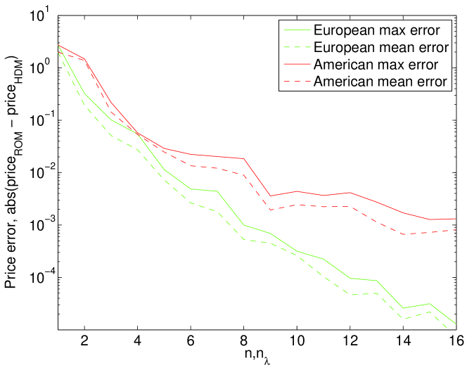
Figure 1: Under the Black–Scholes model the error with respect to the the reduced basis size $n=n_{\lambda}$

4.2 Merton Model

The model parameters for the Merton model are varied in the range:

$$(r,\,\sigma_{s},\,\mu,\,\delta,\,\gamma)\in[0.025,\,0.035]\times[0.35,\,0.45]\times[0.15,\,0.25]\times[0.3,\,0.5]\times[-0.7,\,-0.3].$$ (32)

The price of the European and American options vary roughly in the ranges $[9.50,13.97]$ and $[9.65,14.08]$, respectively. Figure 2 shows the reduction of the maximum and mean errors of the price of these options with the growth of the reduced basis sizes $n=n_{\lambda}$.

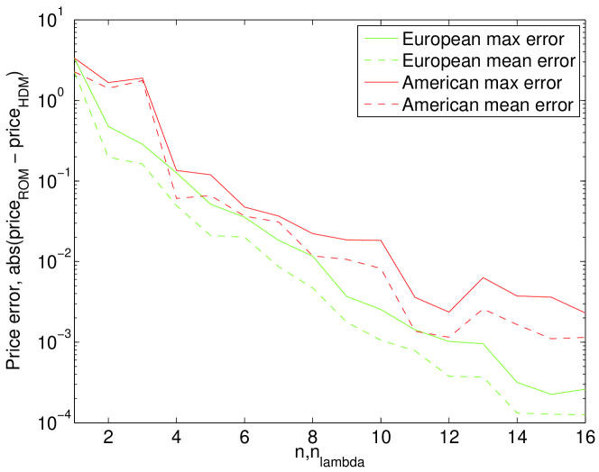
Figure 2: Under the Merton model the error with respect to the the reduced basis size $n=n_{\lambda}$

4.3 Heston Model

The model parameters for the Heston model are varied in the range:

$$(r,\,\kappa,\,\theta,\,\sigma_{v},\,\rho)\in[0.025,\,0.035]\times[3,\,5]\times[0.35^{2},\,0.45^{2}]\times[0.35,\,0.45]\times[-0.75,\,-0.25].$$ (33)

The price of the European and American options vary roughly in the ranges $[8.72,11.88]$ and $[8.87,11.98]$, respectively. Figure 3 shows the reduction of the maximum and mean errors of the price of these options with the growth of the reduced basis sizes $n=n_{\lambda}$.

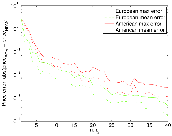
Figure 3: Under the Heston model the error with respect to the the reduced basis size $n=n_{\lambda}$

4.4 Bates Model

The model parameters for the Bates model are varied in the range:

$$\begin{split}(r,\,\kappa,\,\theta,\,\sigma_{v},\,\rho,\,\mu,\,\delta,\,\gamma)\in{}&[0.025,\,0.035]\times[3,\,5]\times[0.35^{2},\,0.45^{2}]\times[0.35,\,0.45]\times\\ &[-0.75,\,-0.25]\times[0.15,\,0.25]\times[0.3,\,0.5]\times[-0.7,\,-0.3].\end{split}$$ (34)

The price of the European and American options vary roughly in the ranges $[9.38,13.95]$ and $[9.53,14.07]$, respectively. Figure 4 shows the reduction of the maximum and mean errors the price of these options with the growth of the reduced basis sizes $n=n_{\lambda}$. We note that for this model essentially the same errors can be obtained based only on $2^{8}=256$ training runs sampling the extreme values of the model parameters.

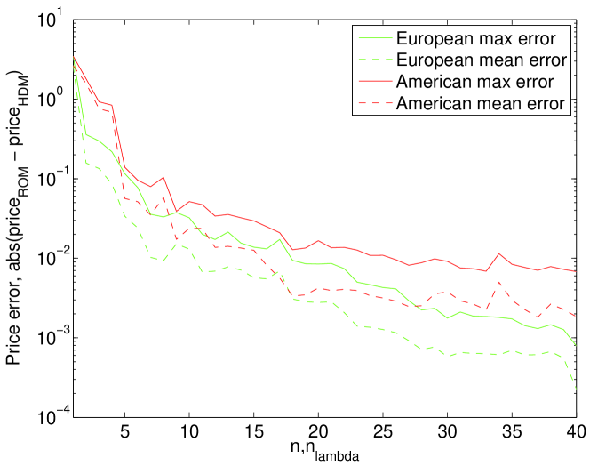
Figure 4: Under the Bates model the error with respect to the the reduced basis size $n=n_{\lambda}$

4.5 Computational Speed-up

For each problem considered, the speed-up factor delivered by its ROM for the online computations is reported in Table 1 for the European option and in Table 2 for the American option. All models are solved in MATLAB on a Intel Xeon 2.6GHz CPU and all CPU times were measured using the tic-toc function on a single computational thread via the -singleCompThread start-up option. A ROM is integrated in time using the same scheme and time-step used to solve its corresponding FOM; see Section 2 for details. The online speed-up is calculated by evaluating the ratio between the time-integration of the FOM and the time-integration of the ROM.

Table 1: For the European option CPU times in seconds for online computations.

	FOM		ROM
Model	unknowns	CPU time	unknowns	CPU time	speed-up
Black–Scholes	8127	0.0011	16	0.00064	1.7
Merton	8127	0.0022	16	0.00084	2.6
Heston	8255	0.1699	40	0.00119	145
Bates	8255	0.3699	40	0.00159	240

Table 2: For the American option CPU times in seconds for online computations.

	FOM		ROM
Model	unknowns	CPU time	unknowns	CPU time	speed-up
Black–Scholes	8127	0.026	16	0.025	1.0
Merton	8127	0.027	16	0.026	1.0
Heston	8255	7.999	40	0.034	232
Bates	8255	8.099	40	0.034	235

5 Conclusions

Reduced order models (ROMs) were constructed for pricing European and American options under jump-diffusion and stochastic volatility models. For American options they are based on a penalty formulation of the linear complementarity problem. The finite difference discretized differential operator is projected using basis resulting from a proper orthogonal decomposition. The grid points for the penalty term are chosen using the discrete empirical interpolation method. In numerical experiments, from two to eight model parameters are varied in a given range. For the one-dimensional Black–Scholes and Merton models about 16 ROM basis vectors were enough to reach 0.1% accuracy for the considered American option. For the European option about 8 basis vectors lead to this accuracy. For the two-dimensional Heston and Bates models about 40 basis vectors were needed to reach the same accuracy for the American option. Slightly less basis vectors lead to the same accuracy for the European option. For these two-dimensional models the computational speed-up was over 200 when the full order model (FOM) and ROM have roughly the same 0.1% accuracy level for the American option. For the European option the solution of the FOM and the ROM under the Bates model required about 0.36 and 0.0015 seconds, respectively. For the American option the solution of the FOM and the ROM for two-dimensional models required about 8 and 0.034 seconds, respectively. With the one-dimensional models the speed-up was negligible. Particularly the results with the Bates model and eight parameters varying are impressive. For one-dimensional models probably for most applications FOMs are sufficiently fast. For two-dimensional models often FOMs are computationally too expensive and in such cases the proposed ROMs can enable the use of these models. Performance of the proposed ROM approach is quite similar to previous approaches based on the NNMF. For example, the maximum ROM price error using 40 basis vectors under the Heston model using the proposed approach and the previous approach based on NNMF is $2.9\times 10^{-3}$, and $4.2\times 10^{-3}$, respectively. While for the Bates model, the maximum ROM price error using 40 basis vectors using the proposed approach and the previous approach based on NNMF is $6.8\times 10^{-3}$, and $4.0\times 10^{-3}$ respectively. A potential application for these ROMs is the calibration of the model parameters based on market data. With a least squares calibration formulation, option prices and their sensitivities can be computed quickly and accurately for varying parameters by employing ROMs.

References

- [1] F. Black, M. Scholes, The pricing of options and corporate liabilities, J. Political Economy 81 (1973) 637–654. doi:10.1086/260062.
- [2] R. C. Merton, Option pricing when underlying stock returns are discontinuous, J. Financial Econ. 3 (1976) 125–144. doi:10.1016/0304-405X(76)90022-2.
- [3] S. Heston, A closed-form solution for options with stochastic volatility with applications to bond and currency options, Rev. Financial Stud. 6 (1993) 327–343. doi:10.1093/rfs/6.2.327.
- [4] D. S. Bates, Jumps and stochastic volatility: Exchange rate processes implicit Deutsche mark options, Review Financial Stud. 9 (1) (1996) 69–107. doi:10.1093/rfs/9.1.69.
- [5] N. Clarke, K. Parrott, Multigrid for American option pricing with stochastic volatility, Appl. Math. Finance 6 (1999) 177–195. doi:10.1080/135048699334528.
- [6] T. Haentjens, K. J. in ’t Hout, ADI schemes for pricing American options under the Heston model, Appl. Math. Finance 22 (3) (2015) 207–237. doi:10.1080/1350486X.2015.1009129.
- [7] S. Ikonen, J. Toivanen, Efficient numerical methods for pricing American options under stochastic volatility, Numer. Methods Partial Differential Equations 24 (1) (2008) 104–126. doi:10.1002/num.20239.
- [8] R. Zvan, P. A. Forsyth, K. R. Vetzal, Penalty methods for American options with stochastic volatility, J. Comput. Appl. Math. 91 (2) (1998) 199–218. doi:10.1016/S0377-0427(98)00037-5.
- [9] Y. d’Halluin, P. A. Forsyth, G. Labahn, A penalty method for American options with jump diffusion processes, Numer. Math. 97 (2) (2004) 321–352. doi:10.1007/s00211-003-0511-8.
- [10] Y. Kwon, Y. Lee, A second-order tridiagonal method for American options under jump-diffusion models, SIAM J. Sci. Comput. 33 (4) (2011) 1860–1872. doi:10.1137/100806552.
- [11] S. Salmi, J. Toivanen, An iterative method for pricing American options under jump-diffusion models, Appl. Numer. Math. 61 (7) (2011) 821–831. doi:10.1016/j.apnum.2011.02.002.
- [12] S. Salmi, J. Toivanen, A comparison and survey of finite difference methods for pricing American options under finite activity jump-diffusion models, Int. J. Comput. Math. 89 (9) (2012) 1112–1134. doi:10.1080/00207160.2012.669475.
- [13] S. Salmi, J. Toivanen, IMEX schemes for pricing options under jump-diffusion models, Appl. Numer. Math. 84 (2014) 33–45. doi:10.1016/j.apnum.2014.05.007.
- [14] J. Toivanen, A componentwise splitting method for pricing American options under the Bates model, in: Applied and numerical partial differential equations, Vol. 15 of Comput. Methods Appl. Sci., Springer, New York, 2010, pp. 213–227. doi:10.1007/978-90-481-3239-3\_16.
- [15] L. V. Ballestra, C. Sgarra, The evaluation of American options in a stochastic volatility model with jumps: an efficient finite element approach, Comput. Math. Appl. 60 (6) (2010) 1571–1590. doi:10.1016/j.camwa.2010.06.040.
- [16] S. Salmi, J. Toivanen, L. von Sydow, Iterative methods for pricing American options under the Bates model, in: Proceedings of 2013 International Conference on Computational Science, Vol. 18 of Procedia Computer Science Series, Elsevier, 2013, pp. 1136–1144. doi:10.1016/j.procs.2013.05.279.
- [17] S. Salmi, J. Toivanen, L. von Sydow, An IMEX-scheme for pricing options under stochastic volatility models with jumps, SIAM J. Sci. Comput. 36 (5) (2014) B817–B834. doi:10.1137/130924905.
- [18] L. von Sydow, J. Toivanen, C. Zhang, Adaptive finite differences and IMEX time-stepping to price options under Bates model, Int. J. Comput. Math. 92 (12) (2015) 2515–2529. doi:10.1080/00207160.2015.1072173.
- [19] A. Antoulas, Approximation of large-scale dynamical systems, Vol. 6 of Advances in Design and Control, Society for Industrial and Applied Mathematics (SIAM), Philadelphia, PA, 2005. doi:10.1137/1.9780898718713.
- [20] P. Benner, S. Gugercin, K. Willcox, A survey of projection-based model reduction methods for parametric dynamical systems, SIAM Rev. 57 (4) (2015) 483–531. doi:10.1137/130932715.
- [21] L. Sirovich, Turbulence and the dynamics of coherent structures. I. Coherent structures, Quart. Appl. Math. 45 (3) (1987) 561–571.
- [22] M. Rewieński, J. White, Model order reduction for nonlinear dynamical systems based on trajectory piecewise-linear approximations, Linear Algebra Appl. 415 (2) (2006) 426–454. doi:10.1016/j.laa.2003.11.034.
- [23] C. Gu, J. Roychowdhury, Model reduction via projection onto nonlinear manifolds, with applications to analog circuits and biochemical systems, in: 2008 IEEE/ACM International Conference on Computer-Aided Design, IEEE, 2008, pp. 85–92. doi:10.1109/ICCAD.2008.4681556.
- [24] J. Barbič, D. L. James, Real-time subspace integration for St. Venant-Kirchhoff deformable models, in: ACM Transactions on Graphics (TOG), Vol. 24, ACM, 2005, pp. 982–990. doi:10.1145/1186822.1073300.
- [25] M. Balajewicz, E. Dowell, B. Noack, Low-dimensional modelling of high-Reynolds-number shear flows incorporating constraints from the Navier-Stokes equation, J. Fluid Mech. 729 (2013) 285–308. doi:10.1017/jfm.2013.278.
- [26] M. Balajewicz, I. Tezaur, E. Dowell, Minimal subspace rotation on the Stiefel manifold for stabilization and enhancement of projection-based reduced-order models for the compressible Navier-Stokes equations, J. Comput. Phys. 321 (2016) 224–241. doi:10.1016/j.jcp.2016.05.037.
- [27] M. Balajewicz, E. Dowell, Stabilization of projection-based reduced-order models of the Navier-Stokes equations, Nonlinear Dynam. 70 (2) (2012) 1619–1632. doi:10.1007/s11071-012-0561-5.
- [28] L. Cordier, B. Noack, G. Tissot, G. Lehnasch, J. Delville, M. Balajewicz, G. Daviller, R. Niven, Identification strategies for model-based control, Exp. Fluids 54 (8) (2013) 1–21. doi:10.1007/s00348-013-1580-9.
- [29] D. Ryckelynck, A priori hyperreduction method: an adaptive approach, J. Comput. Phys. 202 (1) (2005) 346–366. doi:10.1016/j.jcp.2004.07.015.
- [30] S. S. An, T. Kim, D. L. James, Optimizing cubature for efficient integration of subspace deformations, in: ACM Transactions on Graphics (TOG), Vol. 27, ACM, 2008, p. 165. doi:10.1145/1409060.1409118.
- [31] S. Chaturantabut, D. C. Sorensen, Nonlinear model reduction via discrete empirical interpolation, SIAM J. Sci. Comput. 32 (5) (2010) 2737–2764. doi:10.1137/090766498.
- [32] K. Carlberg, C. Bou-Mosleh, C. Farhat, Efficient non-linear model reduction via a least-squares Petrov-Galerkin projection and compressive tensor approximations, Int. J. Numer. Meth. Eng. 86 (2) (2011) 155–181. doi:10.1002/nme.3050.
- [33] D. Amsallem, C. Farhat, Stabilization of projection-based reduced-order models, Int. J. Numer. Meth. Eng. 91 (4) (2012) 358–377. doi:10.1002/nme.4274.
- [34] C. Farhat, P. Avery, T. Chapman, J. Cortial, Dimensional reduction of nonlinear finite element dynamic models with finite rotations and energy-based mesh sampling and weighting for computational efficiency, Int. J. Numer. Meth. Eng. 98 (9) (2014) 625–662. doi:10.1002/nme.4668.
- [35] D. Amsallem, M. J. Zahr, Y. Choi, C. Farhat, Design optimization using hyper-reduced order models, Struct. Multidiscip. O. 51 (4) (2014) 919–940. doi:10.1007/s00158-014-1183-y.
- [36] C. Farhat, T. Chapman, P. Avery, Structure-preserving, stability, and accuracy properties of the energy-conserving sampling and weighting method for the hyper reduction of nonlinear finite element dynamic models, Int. J. Numer. Meth. Eng. 102 (5) (2015) 1077–1110. doi:10.1002/nme.4820.
- [37] O. Burkovska, B. Haasdonk, J. Salomon, B. Wohlmuth, Reduced basis methods for pricing options with the Black-Scholes and Heston models, SIAM J. Financial Math. 6 (1) (2015) 685–712. doi:10.1137/140981216.
- [38] M. Balajewicz, D. Amsallem, C. Farhat, Projection-based model reduction for contact problems, Int. J. Numer. Meth. Eng. 106 (8) (2016) 644–663. doi:10.1002/nme.5135.
- [39] M. Balajewicz, J. Toivanen, Reduced order models for pricing American options under stochastic volatility and jump-diffusion models, in: Proceedings of 2016 International Conference on Computational Science, Vol. 80 of Procedia Computer Science Series, Elsevier, 2016, pp. 734–743. doi:10.1016/j.procs.2016.05.360.
- [40] R. Cont, N. Lantos, O. Pironneau, A reduced basis for option pricing, SIAM J. Financial Math. 2 (1) (2011) 287–316. doi:10.1137/10079851X.
- [41] E. W. Sachs, M. Schu, A priori error estimates for reduced order models in finance, ESAIM Math. Model. Numer. Anal. 47 (2) (2013) 449–469. doi:10.1051/m2an/2012039.
- [42] B. Haasdonk, J. Salomon, B. Wohlmuth, A reduced basis method for the simulation of American options, in: Numerical mathematics and advanced applications 2011, Springer, Heidelberg, 2013, pp. 821–829.
- [43] O. Pironneau, Calibration of options on a reduced basis, J. Comput. Appl. Math. 232 (1) (2009) 139–147. doi:10.1016/j.cam.2008.10.070.
- [44] E. W. Sachs, M. Schu, Reduced order models in PIDE constrained optimization, Control Cybernet. 39 (3) (2010) 661–675.
- [45] E. W. Sachs, M. Schneider, M. Schu, Adaptive trust-region POD methods in PIDE-constrained optimization, in: Trends in PDE constrained optimization, Vol. 165 of Internat. Ser. Numer. Math., Birkhäuser/Springer, Cham, 2014, pp. 327–342. doi:10.1007/978-3-319-05083-6_20.
- [46] E. Ekström, J. Tysk, The Black-Scholes equation in stochastic volatility models, J. Math. Anal. Appl. 368 (2) (2010) 498–507. doi:10.1016/j.jmaa.2010.04.014.
- [47] K. Ito, J. Toivanen, Lagrange multiplier approach with optimized finite difference stencils for pricing American options under stochastic volatility, SIAM J. Sci. Comput. 31 (4) (2009) 2646–2664. doi:10.1137/07070574X.
- [48] D. Amsallem, J. Nordström, Energy stable model reduction of neurons by nonnegative discrete empirical interpolation, SIAM J. Sci. Comput. 38 (2) (2016) B297–B326. doi:10.1137/15M1013870.
- [49] L. von Sydow, L. Höök, E. Larsson, E. Lindström, S. Milovanović, J. Persson, V. Shcherbakov, Y. Shpolyanskiy, S. Sirén, J. Toivanen, J. Walden, M. Wiktorsson, J. Levesley, J. Li, C. Oosterlee, M. Ruijter, A. Toropov, Y. Zhao, BENCHOP – The BENCHmarking project in option pricing, Int. J. Comput. Math. 92 (12) (2015) 2361–2379. doi:10.1080/00207160.2015.1072172.