Haldane phase in the sawtooth lattice: Edge states, entanglement spectrum and the flat band

Abstract

Using density matrix renormalization group numerical calculations, we study the phase diagram of the half filled Bose-Hubbard system in the sawtooth lattice with strong frustration in the kinetic energy term. We focus in particular on values of the hopping terms which produce a flat band and show that, in the presence of contact and near neighbor repulsion, three phases exist: Mott insulator (MI), charge density wave (CDW), and the topological Haldane insulating (HI) phase which displays edge states and particle imbalance between the two ends of the system. We find that, even though the entanglement spectrum in the Haldane phase is not doubly degenerate, it is in excellent agreement with the entanglement spectrum of the Affleck-Kennedy-Lieb-Tasaki (AKLT) state built in the Wannier basis associated with the flat band. This emphasizes that the absence of degeneracy in the entanglement spectrum is not necessarily a signature of a non-topological phase, but rather that the (hidden) protecting symmetry involves non-local states. Finally, we also show that the HI phase is stable against small departure from flatness of the band but is destroyed for larger ones.

I Introduction

Since its introduction by Fisher et al. fisher89 , the bosonic Hubbard model (BHM) and its variants have attracted a great deal of attention due to the rich physics and wide variety of phases and phase transitions it exhibits: incompressible Mott insulator (MI), superfluid (SF), Bose glass in the presence of disorder fisher89 ; charge density wave (CDW), supersolid (SS) and phase separation in the presence of longer range repulsion batrouni14 ; batrouni95 ; batrouni00 ; goral02 ; wessel05 ; boninsegni05 ; sengupta05 ; otterlo05 ; batrouni06 ; yi07 ; suzuki07 ; dang08 ; pollet10 ; capogrosso10 . Interest intensified when trapped atomic condensates where loaded in optical lattices greiner02 where it was shown that the system is governed by the BHM jaksch99 . The high tunability of the interaction strengths, the wide range of lattice geometries that can be realized and the ability to perform very detailed measurements offered access to a very wide range systems and tight binding Hamiltonians of great interest in the study of strongly correlated systems.

Increasingly, over the last several years, the physics of strongly correlated quantum systems has focused on the existence and properties of unconventional phases and phase transitions. For example, when the extended one-dimensional Bose Hubbard model (EBH) is at full filling and the contact interaction dominates, the system is in the MI phase with one particle per site. As the near neighbor interaction is increased, quantum fluctuations create holes and doublons, typically leading to three kinds of sites: empty, singly occupied and doubly occupied. One can then approximate the model by the spin-$1$ Heisenberg chain with $S_{z}=1,0,-1$ for the doubly, singly and empty sites. This led to the discovery altman06 ; altman08 that at full filling, the one dimensional extended BHM supports, in addition to the SF, MI and CDW phases, a topological phase characterized by a nonlocal string order parameter and edge states. This phase, called the Haldane insulator (HI), is closely related to the Haldane phase haldane83 appearing in integer spin chains and realized in the AKLT state aklt87 ; kt92 . The phase diagram of this model was elaborated and the excitation spectra studied using quantum Monte Carlo (QMC) simulations and density matrix renormalization group (DMRG) calculations rossini12 ; ggb13 ; ggb14 ; ggb16 . Another situation where unconventional phases may be encountered is that of strong geometrical frustration, for example in the particle kinetic energy. If the hopping term in the Hamiltonian is frustrated in a particular way, the lowest band can become flat resulting in a huge degeneracy of states into which the particles may condense. This degeneracy changes the behavior of the particles when their density is sufficiently low (or when there is no interaction between them): The particles are localized in extended geometrical structures due to interference effects of the hopping terms. What happens when interaction is present and the particle filling exceeds a critical value dictated by the lattice geometry was treated by several authorshuber10 ; takayoshi13 ; tovmasyan13 . A general approach used in these references is to project the Hamiltonian onto the flat band resulting in an effective low energy Hamiltonian which depends only on the interaction. For example, in Ref.[huber10, ], the sawtooth and the kagome lattices were treated in this way. For the sawtooth lattice, the effective projected Hamiltonian describes bosons hopping on a one-dimensional lattice and interacting with each other. The question then arises if, under certain situations, this model can support a topological phase, such as the HI, as happens in the extended one-dimensional BHM mentioned above.

This is the main question which we will address in this work. We will show, with DMRG calculations, that by adding an extended interaction term to the model studied in Ref.[huber10, ], and when the system has a flat band and is at half filling, the charge and neutral gaps behave in a way reminiscent of the HI. We then show the presence of edge states and imbalance in the number of particles on the two ends of the system (with open boundary conditions) which confirms the existence of the HI. We also show that, contrary to the usual situation, the entanglement spectrum does not exhibit a doubly degenerate ground state in the Haldane phase. We then demonstrate that this behavior persists in a finite interval of geometric frustration around the flat band but disappears if the frustration is far from what is needed for flatness.

The paper is organized as follows. In section II we present the model and review the results of Ref. huber10, . In section III we present our DMRG results for the gaps and density profiles and discuss the various phases found at half filling. Topological aspects of the edge states are presented and discussed in section IV while the entanglement spectrum is discussed in section V. The phase diagrams when the lowest band is dispersive but still almost flat are presented in section VI followed by our conclusions in section VII.

II Model

We will study the BHM on the sawtooth lattice, Fig.1, and governed by the Hamiltonian

$$H = \sum_{\langle ij\rangle}|t_{ij}|\left(a_{i}^{\dagger}a_{j}^{\phantom{\dagger}}+{\rm H.c}\right)+\frac{U}{2}\sum_{i}n_{i}(n_{i}-1)$$ (1)

$$+V\sum_{\langle ij\rangle_{B}}n_{i}n_{j},$$

where $\langle ij\rangle$ denotes near neighbors and $\langle ij\rangle_{B}$ near neighbors of the $B$ type; the operators $a_{i}$ and $a_{i}^{\dagger}$ are destruction and creation operators on site $i$ and satisfy the usual bosonic commutation relations. $n_{i}$ is the number operator on site $i$ and $t_{ij}$ is the hopping parameter between near neighbor sites. We will take $t_{ij}=t$ for hops between two B sites (see Fig.1) and $t_{ij}=t^{\prime}$ for hops between A and B sites. The contact interaction strength is $U$ and the near neighbor interaction is $V$ both of which are taken to be repulsive. Note that the near neighbor repulsion is only between neighboring $B$ sites for reasons to be discussed below.

The kinetic part of the Hamiltonian, Eq.(1), can be easily diagonalizedhuber10 giving the band energies

$$\epsilon_{\pm}(k)=\cos(ka)\pm\sqrt{t^{2}\cos^{2}(ka)+2t^{\prime 2}\cos(ka)+2t^{\prime 2}}.$$ (2)

When $t^{\prime}=\sqrt{2}t$, the lowest band becomes flat and we get,

$$\epsilon_{\pm}(k)=\begin{cases}\quad\phantom{-}2t\left(1+\cos(ka)\right),\\ \quad-2t,\end{cases}$$ (3)

where $a$ is the distance between two $B$ sites.

If a particle is now introduced in the system, it will be localized on three sites, in the shape of V, due to the interference effects of frustration. These sites are shown in thick (red) V-shaped structures in Fig.1. The localized states are given by,

$$|V_{i}\rangle=\frac{1}{2}\left(\sqrt{2}a_{B,i}^{\dagger}-a_{A,i-1}^{\dagger}-a_{A,i}^{\dagger}\right)|0\rangle,$$ (4)

where, on average, a $B$ site is occupied by $1/2$ a particle and each of the two $A$ sites by $1/4$. It is clear from Fig.1 that even in the presence of interaction, if the total number of particles is less than or equal to $1/4$ of the number of sites, these localized states are eigenstates of $H$. If the particle density exceeds the critical density of $1/4$, the V states will start sharing $A$ sites and, therefore, interacting. The energy per particle will no longer be $-2t$. Figure 1 shows the configuration of V’s for the case of maximum filling without interacting and exhibits a CDW of V’s alternately empty and occupied by one particle.

Figure 1: (Color online) The sawtooth lattice. Sites at the bases of the triangles are denoted $B$ and apex sites are $A$. The localized state wavefunction has positive amplitude on the $B$ sites and negative on the $A$ sites (see text). The thick (red) lines in the form of V are the states localized in the flat band. The sites labeled $A$ and $B$ belong to the same unit cell. Our convention for the lattice names, i.e. AA, BB and AB, indicates the type of site at each end of the lattice with open boundary conditions.

The states $|V_{i}\rangle$ are linearly independent and complete in the flat band subspace but they are not orthogonal. For this reason, we use Wannier states to define a set of localized orthogonal states forming a complete basis. In general, denoting by $w_{n\,X_{p}}(x)$ the Wannier function for the band $n$ localized around the position $X_{p}$, the Wannier states $|w_{n\,X_{p}}\rangle$ give rise to an orthogonal basis if and only if the centers $X_{p}$ are on a Bravais lattice. In that case, one can express the creation operators $a^{\dagger}_{i}$ as functions of the creation operator $W^{\dagger}_{n\,X_{p}}$, i.e. creating a boson in the Wannier state $|w_{n\,X_{p}}\rangle$:

$$a^{\dagger}_{i}=\sum_{n\,X_{p}}w^{*}_{n\,X_{p}}(x_{i})W^{\dagger}_{n\,X_{p}},$$ (5)

where $x_{i}$ is the position of the site $i$. The projection of the operators on a given band $n$ is made by keeping, in the preceding sum, the Wannier operators for that band only: $a^{\dagger}_{i}\approx\sum_{X_{p}}w^{*}_{n\,X_{p}}(x_{i})W^{\dagger}_{n\,X_{p}}$.

In the present case, the projection on the flat band leads to

$$a^{\dagger}_{Bi} \approx \sum_{j}f_{B}^{*}(j-i)W^{\dagger}_{f\,j}$$

$$a^{\dagger}_{Ai} \approx \sum_{j}f_{A}^{*}(j-(i+1/2))W^{\dagger}_{f\,j},$$ (6)

where the Wannier state $|w^{\dagger}_{f\,j}\rangle$ has been chosen to be localized around the $B$ site at position $ja$. Later, we will also need the expression of the Wannier operators as a function of the operators $a^{\dagger}_{Bi}$ and $a^{\dagger}_{Ai}$:

$$W^{\dagger}_{f\,j}=\sum_{i}\left(f_{B}(j-i)a^{\dagger}_{Bi}+f_{A}(j-(i+1/2))a^{\dagger}_{Ai}\right).$$ (7)

From the band structure, one can derive the amplitude of the Wannier function at the $B$ and $A$ sites:

$$f_{B}^{*}(p) =-\frac{2}{\pi}\int_{0}^{+\pi/2}d\theta\,\frac{\cos(2p\theta)}{\sqrt{1+2\cos^{2}(\theta)}}$$ (8)

$$f_{A}^{*}((p-1/2)) =\frac{2}{\pi}\int_{0}^{+\pi/2}d\theta\,\frac{\sqrt{2}\cos((2p-1)\theta)\cos(\theta)}{\sqrt{1+2\cos^{2}(\theta)}}.$$

The Wannier function on the flat band is plotted in Fig. 2. Note that our definition of these Wannier states differs somewhat from that of reference [huber10, ].

Figure 2: (Color online) Density profile of the Wannier function, see Eq. (7), and of the V-shape, see Eq. (4). centered around the site $B_{i}$. The Wannier function is normalized to one, with a total density probability 0.58 on the $B$ sites and 0.42 on the $A$ sites.

Using DMRG calculations on the original and the effective Hamiltonians, Ref.[huber10, ] showed, for $V=0$, that when the system is doped slightly above the critical density of $1/4$, the CDW melts yielding a SF with a momentum distribution peaking at a nonzero value which depends on the doping.

Here, we are interested in the phases and phase transitions of this system at half filling when the near neighbor repulsion, $V$, is included. Specifically, the questions we address here are: Will the half filled system admit a MI phase of V’s sharing $A$ sites? Will the system admit a CDW phase with alternating vacant and doubly occupied V’s? And, will the system admit a HI phase sandwiched in between these two?

III DMRG: Phase diagram at half filling

To address the above questions, we use the DMRG codes in the ALPSalps library to calculate density profiles and the neutral and charge energy gaps at half filling. We take $t=1$ to fix the energy scale and focus attention on two values of the contact interaction, $U=1/2,1$, and study the system as the near neighbor repulsion, $V$, is varied. Most of our results are for the flat band case, $t^{\prime}=\sqrt{2}t$. The $t^{\prime}\neq\sqrt{2}t$ will be addressed in section VI. We perform the calculations for several system sizes, $L=40,80,120,160,200$ (number of sites is $2L$) with open boundary conditions and a maximum number of boson per state $N_{max}=3$. The neutral gap, $\Delta_{n}$, is calculated by targeting the ground and the first excited states in the DMRG calculation. We typically keep $300$ states in the DMRG calculation and we have verified that keeping more (up to $600$ states) or increasing $N_{max}$ does not change the results. The charge gaps, $\Delta_{c}$, are calculated using the energies at half filling and at half filling doped with one particle and doped with one hole,

$$\Delta_{c}=E(N_{1/2}+1)+E(N_{1/2}-1)-2E(N_{1/2}),$$ (9)

where $N_{1/2}$ is the number of particles at half filling.

Since we use open boundary conditions, our convention for the lattice names, i.e. AA, BB and AB, indicates the type of site at each end of the lattice and since the lattice is frustrated, special care must be taken in order to observe the various phases. More precisely, in the following, we will show that, at half filling, the system exhibits three types of insulating phases: Mott, Haldane, and CDW phases. In order to compute the gap values, one needs to be able to lift the degeneracy among the different ground states. As for the EBH on a 1D chain, this is done by adding a chemical potential at each edge, but, since the “natural” local states after projection on the flat band are the V-shaped structures (or the Wannier function), the boundary conditions must be matched in terms of these local states. In particular, adding a large positive chemical potential on a $B$ site at one edge (and on the neighboring $A$ site, if the lattice ends with an $A$ site) more or less amounts to imposing a vanishing density on the V-shape localized on that $B$ site; on the other hand, adding a large negative chemical potential on either ending $B$ (and on the neighboring $A$) site does not correspond to getting a fixed number of bosons in the V-shape localized on this $B$ site. In other words, we do not have a simple way to impose on the ground state to be in a Fock state in the V-shape (or Wannier) basis at the edge. This is in a sharp contrast with the EBH on a 1D-chain, for which a large negative chemical potential on a given site amounts to fixing the state on that site to a Fock state with $N_{max}$ bosons.

From that point of view, our strategy was to compare the results for the densities, gap values and correlation functions for different lattice types, i.e. AA, BB and AB and different boundary conditions, i.e. adding or not a large chemical potential at each edge. In what follows, we adopt the following conventions: a lattice size $L$ always means a lattice with $(L+1)$ $B$-sites, an AA lattice has then $(L+2)$ $A$-sites whereas a BB lattice has $L$ $A$-sites. Then, it turns out that, for the different phases, the proper choice of the lattice type, boundary conditions and the number of bosons that give the correct charge and neutral gaps is are follows:

• MI phase (single ground state): AA lattice with $L+1$ bosons and no additional chemical potential.

• CDW insulating phase (two degenerate ground states): BB lattice with $L$ bosons, $L$ even and one large additional chemical potential on both the first and last B sites.

• HI phase (four degenerate ground states): BB lattice with $L$ bosons and one large additional chemical potential on both the first and last B sites.

We confirmed that the preceding situations yield correct values for the gaps by comparing with the gap values obtained with DMRG, for $L=40$, under periodic boundary conditions where the above issues do not arise. Larger sizes with periodic boundary conditions do not converge properly with DMRG.

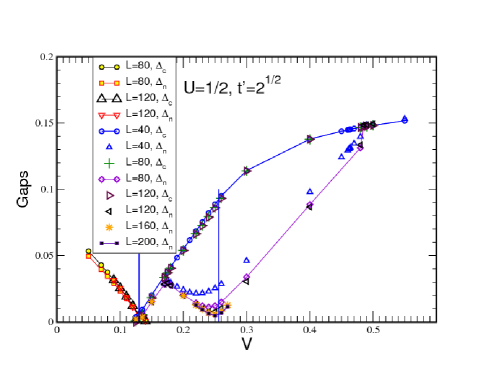
Figure 3: (Color online) DMRG results for the charge, $\Delta_{c}$, and neutral, $\Delta_{n}$, gaps as functions of the near neighbor repulsion, $V$, for $U=1/2$, $t^{\prime}=\sqrt{2}t$ (flat band) at half filling. The vertical lines show the locations of the MI-HI ($V\approx 0.13$) and the HI-CDW ($V=0.256$) transitions (see text).

Figure 3 shows, for several lattice sizes, $\Delta_{c}$ and $\Delta_{n}$ as functions of $V$ for $U=1/2$ and $t^{\prime}=\sqrt{2}$ at half filling. For $V<0.13$, $\Delta_{c}=\Delta_{n}$ and both gaps vanish at $V\approx 0.13$ indicating a quantum phase transition at that point. This behavior of the gaps is indicative of the incompressible MI phasealtman06 . For $V>0.13$, the gaps first increase together, then at $V\approx 0.175$, $\Delta_{n}$ starts to decrease while $\Delta_{c}$ continues increasing. $\Delta_{n}$ then reaches another minimum, which approaches zero as $L$ increases, then starts to increase again tending toward $\Delta_{c}$. This behavior of $\Delta_{n}$ suggests the presence of the HI phase between its two minima. The second minimum of $\Delta_{n}$ is sensitive to finite size effects. We show in Fig.4 how the critical value of $V$ is obtained by extrapolating the value of the minimum to $L\to\infty$. This yields $V_{crit}=0.256$. Therefore, for $0.13\leq V\leq 0.256$ the system is in the Haldane insulating phase. To confirm that this is indeed a HI phase, one could calculate the string order parameteraltman06 ; altman08 ; rossini12 ; ggb13 ; ggb14 ; ggb16 by using the Wannier operators as the “site” operators. However, the nonlocality of the Wannier states leads to extremely complicated expressions in terms of the local operators $a_{i}$, which makes it impractical to compute this Wannier-string order parameter. Instead, we will confirm below the nature of this HI phase by studying topological properties such as the presence of edge states and the entanglement spectrum. For $V>0.256$ the system is in the CDW phase as we will see by examining the density profiles below. Figure 5 shows similar behavior to Fig.3 but for $U=1$.

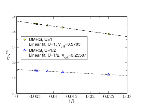
Figure 4: (Color online) The location of the minimum of $\Delta_{n}$ is sensitive to finite size effects. The value of $V$ where $\Delta_{n}$ reaches its minimum is extrapolated to $1/L\to 0$ to obtain the HI-CDW transition value.

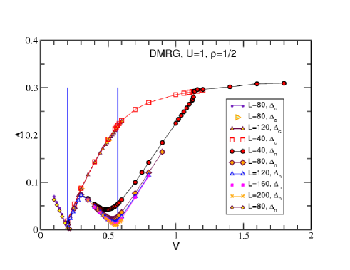
Figure 5: (Color online) DMRG results for the charge, $\Delta_{c}$, and neutral, $\Delta_{n}$, gaps as functions of the near neighbor repulsion, $V$, for $U=1$, $t^{\prime}=\sqrt{2}t$ (flat band) at half filling. The vertical lines show the locations of the MI-HI ($V\approx 0.2$) and the HI-CDW ($V=0.571$) transitions (see text).

The density profiles give additional information on the various phases. In order to show the density profile of the sawtooth lattice as a two-dimensional plot, we assigned integer (half odd integer) labels to the $B$ ($A$) sites. Figure 6 shows the density profile, $n_{i}$, in the MI phase for $U=1/2$ and $V=0.11$. We see that in the bulk, i.e. away from the ends of the system, the average filling of an $A$ site is $\langle n_{A}\rangle=0.59$ while for a $B$ site it is $\langle n_{B}\rangle=0.41$. As $V$ is decreased, $\langle n_{A}\rangle$ and $\langle n_{B}\rangle$ approach $1/2$. This is easy to understand if one recalls the basic localized structure discussed above. In such a localized state, the $B$-site has an average occupation $1/2$ and the $A$-site has $1/4$. At half filling (the case we are considering here) the system is full of touching V’s, so now the average $A$ filling is $1/2$ too. The near neighbor repulsion between $B$ sites disfavors $B$ occupation thus pushing $\langle n_{B}\rangle$ down while the value of $\langle n_{A}\rangle$ increases. This will be discussed further in section V.

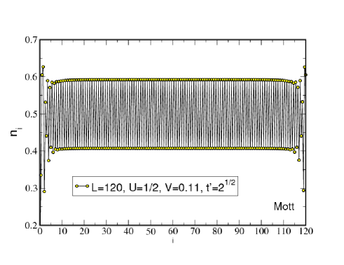
Figure 6: (Color online) Density profile in the MI phase. The $B$ sites are labeled by integer valued site index $i$ while the $A$ sites are labeled by half odd integer. Away from the boundaries, average $B$-site occupation is $0.41$ while that of $A$-sites is $0.59$.

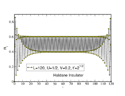
Figure 7: (Color online) The density profile in the HI phase. In the bulk, away from the ends of the system, $\langle n_{A}\rangle=0.6$ and $\langle n_{B}\rangle=0.4$. Near its ends, the system exhibits evidence of edge states whose penetration into the system depends on the value of $V$. See text.

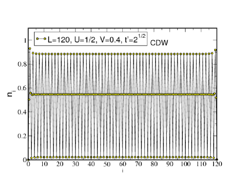
Figure 8: (Color online) The density profile in the CDW phase. $\langle n_{A}\rangle\approx 0.55$ while $\langle n_{B}\rangle$ alternates between almost empty sites, $\langle n_{B}\rangle\approx 0.022$, and $\langle n_{B}\rangle\approx 0.88$ indicating a CDW of V structures (see Fig.1).

Figure 7 shows the density profile in the HI phase, between the two minima of $\Delta_{n}$. In the bulk, away from the ends of the system, $\langle n_{A}\rangle=0.6$ and $\langle n_{B}\rangle=0.4$. Closer to the ends of the system we see evidence of edge states both in the $B$-site and the $A$-site density profiles. In this figure, the edge states extend around 40 sites into the system. This penetration depends on $V$, it decreases as $V$ is taken closer to the MI-HI transition and increases when $V$ is taken closer to the HI-CDW transition. This will be discussed in more detail in sections IV and V. The presence of the edge states is added confirmation that the phase between the two minima of $\Delta_{n}$ is indeed HI.

For $V>0.256$, the system is in the CDW phase: $A$-sites have a constant occupation while $B$-sites alternate between high and low filling. In Fig.8, $V=0.4$, we have $\langle n_{A}\rangle\approx 0.55$ and $\langle n_{B}\rangle$ alternates between almost empty sites $\langle n_{B}\rangle\approx 0.022$ and $\langle n_{B}\rangle\approx 0.88$. As $V$ increases, the occupation of the low-filling $B$-sites decreases further. Roughly speaking, this can be understood in terms alternating doubly occupied V’s, in analogy with the alternating doubly occupied sites in the CDW phase of the one-dimensional BHM on a simple chain.

As explained above, the gap behavior and the density profiles are very reminiscent of the MI-HI-CDW transitions in the usual EBH modelaltman06 ; altman08 ; rossini12 ; ggb13 ; ggb14 ; ggb16 . To emphasize this point, we have used Eq. (7) to compute the average density in the Wannier states. More precisely, we have computed $\langle W^{\dagger}_{f\,i}W^{\phantom{\dagger}}_{f\,i}\rangle$ where $i$ represents the center of the Wannier state, see Fig. 2. The corresponding density profiles in the MI, HI and CDW phases are shown in Figs. 9,10 and 11 respectively. As expected, in the MI the density profile is flat with unit filling, whereas in the HI, the profile exhibits nice edge states at the boundaries and a uniform density in the bulk (unit filling). On the contrary, in the CDW, the density alternates between almost empty sites, $\langle n_{B}\rangle\approx 0.18$ and $\langle n_{B}\rangle\approx 1.82$. Even though the density profile looks very simple in the MI phase, it is not just given by a naive mean-field ansatz consisting of the tensor product of singly occupied Wannier functions:

$$|\mathrm{MI}\rangle=\otimes_{i=1}^{L}|1\,i\rangle,$$ (10)

where $|n\,i\rangle$ is the Fock state having $n$ bosons in the Wannier state centered around the $B$ site $i$. Indeed, using Eq. (7) one can compute the average local densities, $\langle\mathrm{MI}|\hat{n}_{A}|\mathrm{MI}\rangle$ on $A$ sites and $\langle\mathrm{MI}|\hat{n}_{B}|\mathrm{MI}\rangle$ on $B$ sites. This yields $\langle n_{A}\rangle\approx 0.42$ and $\langle n_{B}\rangle\approx 0.58$. These values actually correspond to the total probability density on $A$ and $B$ sites of a single Wannier function and are very different from the ones computed from the ground state, i.e. $\langle n_{A}\rangle=0.59$ and $\langle n_{B}\rangle=0.41$. This strong discrepancy between the ground state of the system and the mean-field ansatz given by Eq. (10) emphasizes that the doublon-holon states (in the Wannier basis) actually have a large contribution to the ground state in the MI phase.

Figure 9: (Color online) Wannier basis density profile in the MI phase, $U=0.5$, $V=0.05$. The average density is equal to 1. The small oscillations at both ends reflect the truncation of the Wannier function due to the boundary.

Figure 10: (Color online) Wannier basis density profile in the HI phase $U=0.5$, $V=0.17$. In the bulk, away from the ends of the system, the average density is one. Near its ends, the system exhibits clear evidence of edge states whose penetration into the system depends on the value of $V$. Due to the boundary conditions (see text), the effective charge of each edge state is $-1/2$.

Figure 11: (Color online) Wannier basis density profile in the CDW phase $U=0.5$, $V=0.4$. The density alternates between almost empty sites ($\langle n_{B}\rangle\approx 0.18$ and $\langle n_{B}\rangle\approx 1.82$ indicating a clear CDW in the Wannier states.

IV Edge states

A feature of the topological Haldane phase, as typified by the AKLT state, is the appearance of edge states when the system has open boundaries. Depending on the boundary conditions, the edge states that appear in the usual EBH on a 1D-chain can exhibit either an excess or a deficit of half a boson compared to the total number of sites occupied by the edge states.

In the sawtooth lattice case, calculating the number of particles on the left and right halves of the system in Figs. 6 and 8 we find balanced populations and, therefore, no topological effects in the MI and CDW phases. However, the situation is different in the case of Fig. 7 where we find $59.8$ particles on the left side and $60.2$ on the right. We verified this is not a finite size effect by doing the same calculations for $L=160,200$ and for several $V$ values and also keeping more states in the DMRG calculation. In all cases we found the same imbalance by $\pm 0.2$ particles relative to half filling. This value of $0.2$ agrees very well with $\langle n_{B}\rangle/2$, i.e. as if half the system loses half the occupation of a single $B$ site which goes to the other half of the system.

This becomes even clearer by examining the edge states directly in the Wannier basis, i.e. using Eq. (7) to compute $\langle W^{\dagger}_{f\,i}W^{\phantom{\dagger}}_{f\,i}\rangle$ where $i$ represents the centre of the Wannier state as plotted in Fig. 10, which resembles very closely the usual EBH on a 1D chain. More precisely, as explained in Sec. II, the BB lattice in our simulations amounts to imposing a vanishing density on both B-sites, which is then analogous to the usual EBH on a 1D chain with vanishing densities at the end. In that situation, the HI ground state is obtained when the number of bosons is one less than the total number of sites, such that, after splitting the system in two parts, each edge state contains a half-boson less than the number of sites in their respective parts. Indeed, in our case, the total number of Wannier “sites”, is $121$, but the total number of bosons $N=120$, because of the vanishing densities at both boundaries. Actually, the total density in the Wannier states is $119.74$ because of the truncation of the Wannier function at the boundaries. When splitting the system in two parts, say the left one with 61 sites and the right one with 60 sites, the total number of bosons is 60.37 to the left and is 59.37 to the right. As one can readily verify, the $0.74$ boson has been split in two between the left and the right parts. Finally, since the average density in the bulk is equal to unity, changing the splitting point would only change these numbers by integer values without affecting the fractional part. This analysis shows the HI phase which we have found in our model, genuinely exhibits edge states with a fractional filling.

In order to bring out more clearly these edge states in our DMRG results, we subtract the bulk values of $\langle n_{A}\rangle$ and $\langle n_{B}\rangle$ from the occupations of the $A$ and $B$ sites in the density profiles in the HI phase. In other words, for all integer sites (i.e. $B$-sites) we subtract the bulk value of $\langle n_{B}\rangle$, and for all half odd integer sites (i.e. $A$-sites) we subtract the bulk value of $\langle n_{A}\rangle$. This yields the shifted density profiles in Fig.12. The figure, which resembles Fig. 10, shows that close to the MI-HI transition ($V=0.135$) the edge states extend a few sites into the system on each side. As $V$ increases and the system approaches the HI-CDW transition, the edge states extension increases until, for a fixed system size, $L$, the two edge states start to overlap. When this happens, a larger system is needed to get precise results. When the HI-CDW transition point is reached, $\Delta_{n}$ vanishes and the system makes the transition to the CDW phase.

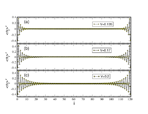
Figure 12: (Color online) The shifted density profiles, $\langle n_{i}\rangle^{\prime}$, in the HI phase (see text) for $L=120$, $U=1/2$. The extent of the edge state into the system increases as $V$ approaches the HI-CDW transition value. The envelope is exponential.

The envelopes of the edge states decay exponentially as is shown in Fig.13. The exponent decreases as $V$ increases toward the HI-CDW transition and the edge states penetrate deeper into the system.

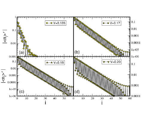
Figure 13: (Color online) The absolute value of the shifted density profile for the left half of the system at four values of $V$. The semi-log plot shows that the envelope of the edge states is exponential and that the exponent decreases as the HI-CDW transition is approached.

V Entanglement spectrum and Wannier functions

Since the density profiles and the gaps agree very well with a Haldane-like topological phase, we have also looked at the properties of the entanglement spectrum in the different phases using DMRG and imaginary time TEBD. Interestingly, and contrary to the usual EBH model, we found no degeneracy in the entanglement spectrum. At first glance, the absence of degeneracy may appear puzzling. However, it turns out that this feature does not mean that the phase is not topological; in fact it is the consequence of the non-locality of the Wannier state. Indeed it also appears in the AKLT-like matrix product state built on the Wannier states rather than the local states. More precisely, we consider the following family of states:

$$\left[\begin{array}[]{cc}|\Psi_{-+}\rangle&|\Psi_{++}\rangle\\ |\Psi_{--}\rangle&|\Psi_{+-}\rangle\end{array}\right]=\otimes_{i=1}^{L}\left[\begin{array}[]{cc}\cos\theta|1,i\rangle&\sin\theta|2,i\rangle\\ \sin\theta|0,i\rangle&\cos\theta|1,i\rangle\end{array}\right],$$ (11)

where $|n\,i\rangle$ denotes the Fock state having $n$ bosons in the Wannier state centered around the $B$ site $i$. Each of the four preceding states has unit average density and a doubly degenerate entanglement spectrum when computing the density matrix in the Wannier basis. Expanding the Wannier states in the local states (see Eq. (7)), one can, in principle, compute the expression of $|\Psi_{\pm\,\pm}\rangle$ in the local Fock states:

$$|\Psi_{\pm\,\pm}\rangle=\sum_{\{n_{A},n_{B}\}}C^{\pm\,\pm}_{\{n_{A},n_{B}\}}|\{n_{A},n_{B}\}\rangle,$$ (12)

where $\{n_{A},n_{B}\}$ is a shorthand notation for a particular configuration of the occupation numbers in the different sawtooth lattice sites, i.e. $(\cdots,n_{A_{i}},n_{B_{i}},\cdots)$, and $|\{n_{A},n_{B}\}\rangle$ is the Fock state corresponding to this configuration. Actually, since the number of coefficients grows exponentially, exact numerical values can only be obtained for rather small sizes $L\approx 10$. On the other hand, it is very simple to build the matrix product state (MPS) with fixed bond dimension (in the local Fock states $|\{n_{A},n_{B}\}\rangle$) associated with these AKLT-like states. We have verified that for small system size, the MPS approximation has the same properties (density) as the exact expression given by Eq. (12). For the values $\cos\theta=1/\sqrt{3}$ and $\sin(\theta)=\sqrt{2/3}$, the density profile of the state $|\Psi_{--}\rangle$ is given in Fig. 14 for $L=50$. Away from the boundaries, the average density on the $A$ site is 0.61 and 0.39 on the $B$ site; these values are extremely close to the DMRG ground state ones in the HI phase, see Fig. 7. More saliently, we find that the entanglement spectrum obtained by splitting the state in the left and right parts in the local basis is uniform and the largest eigenvalues are: $(0.69,0.24,0.051,0.014)$. Obviously, the spectrum is not degenerate which emphasizes the impact of the non-locality of the Wannier function on the properties of the entanglement. In addition, the values found for the AKLT-like state are extremely close to the ground state ones in the HI phase $(0.690.230.0460.02)$, which indirectly proves that for $U=0.5$ and $0.13<V<0.256$, the system does exhibit a Haldane phase, but built on the Wannier states. Finally, one can compute the number of bosons of the left and right edge states of these AKLT states, as in in section IV for the ground state. Here again, one finds that the left part has 25.2 particles and the right side has 24.8 particles, the imbalance is $\pm 0.2$ bosons, exactly as for the DMRG ground state.

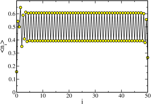
Figure 14: (Color online) Density profile of the AKLT-like state $|\Psi_{--}\rangle$. Away from the boundaries, the average density on the $A$ site is 0.61 and 0.39 on the $B$ site; these values are extremely close to the DMRG ground state ones in the HI phase. In addition, the edge states contain a fractional number of bosons, the imbalance being $\pm 0.2$ like for the ground state of our model.

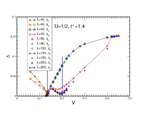
Figure 15: (Color online) DMRG results for the charge, $\Delta_{c}$, and neutral, $\Delta_{n}$, gaps as functions of the near neighbor repulsion, $V$, for $U=1/2$, $t^{\prime}=1.4t$ at half filling. The vertical lines show the locations of the MI-HI ($V\approx 0.136$) and the HI-CDW ($V=0.2$) transitions.

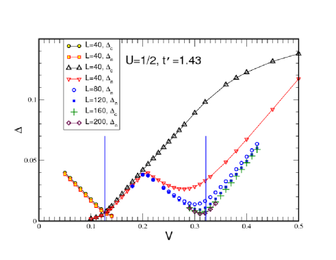
Figure 16: (Color online) DMRG results for the charge, $\Delta_{c}$, and neutral, $\Delta_{n}$, gaps as functions of the near neighbor repulsion, $V$, for $U=1/2$, $t^{\prime}=1.43t$ at half filling. The vertical lines show the locations of the MI-HI ($V\approx 0.128$) and the HI-CDW ($V=0.322$) transitions.

VI Nearly flat band

So far, we have studied the system only in the flat band case, $t^{\prime}=\sqrt{2}t$. The question we address now is: Does the phase diagram, in particular the HI phase, survive for any value of $t^{\prime}$? We studied in detail the phase diagram for two values, $t^{\prime}=1.4$ (i.e. smaller than $\sqrt{2}$) and $t^{\prime}=1.43$ (i.e. larger than $\sqrt{2}$). The results, Figs.15 and 16, show that the gaps behave in a very similar manner to the $t^{\prime}=\sqrt{2}$ case, in particular the behavior of $\Delta_{n}$ indicates that the HI phase persists. Furthermore, we verified that the edge states are present and behave as for the case of $t^{\prime}=\sqrt{2}t$.

However, it is clear from Fig.15 and Fig.3 that the HI phase gets narrower with the smaller value of $t^{\prime}$. In fact, the HI phase does not exist for $t^{\prime}=1.3$. On the other hand, Fig.16 shows that the HI phase expands for the larger value of $t^{\prime}$. However, this expansion does not continue as $t^{\prime}$ continues to increase; for a large enough value $\Delta_{n}$ will not dip down to zero. The CDW phase will be reached directly from the MI phase. This is the case for $t^{\prime}=1.5$.

This shows that the phase diagram, in particular the presence of the topological HI phase, is robust and persists in a finite (but narrow) range of values of $t^{\prime}$ centered at the flat band value, $t=\sqrt{2}$. We also observed the same behavior for $U=1$.

VII Conclusion and outlook

In summary, we have studied the phase diagram of the half filled Bose-Hubbard system in the sawtooth lattice in the situation where the geometric frustration in the hopping term produces a flat band. We have shown that, in the presence of contact and near neighbor repulsion, three phases exist: Mott insulator (MI), charge density wave (CDW), and the topological Haldane insulating (HI) phase. In particular, we have shown that in the HI phase, even though the entanglement spectrum is not doubly degenerate, it is in excellent agreement with the entanglement spectrum of the Affleck-Kennedy-Lieb-Tasaki (AKLT) state built in the Wannier basis associated with the flat band. This emphasizes that the abscence of degeneracy in the entanglement spectrum is not necessarily a signature of a non-topological phase, but rather that the (hidden) protecting symmetry involves non-local states. Finally, we have also shown that, at fixed interactions, the HI phase is stable against small departure from flatness of the band but is destroyed as the band dispersion becomes stronger.

For future work, it would be interesting to find an efficient way to compute the string order in the Wannier basis and to show that it vanishes at the MI-HI transition. In addition, it would be illuminating to study the excitations of the system, and, along the preceding line, to show that the elementary excitations correspond to domain walls in the string order.

- (1) M.P.A. Fisher, P. B. Weichman, G. Grinstein and D. S. Fisher, Phys. Rev. B40, 546 (1989).
- (2) G. G. Batrouni, V. G. Rousseau, R. T. Scalettar, and B. Grémaud Phys. Rev. B 90, 205123 (2014).
- (3) G. G. Batrouni, R. T. Scalettar, G. T. Zimanyi and A. P. Kampf, Phys. Rev. Lett. 74, 2527 (1995).
- (4) G. G. Batrouni and R. T. Scalettar, Phys. Rev. Lett. 84, 1599 (2000).
- (5) K. Gral, L. Santos and M. Lewenstein, Phys. Rev. Lett. 88, 170406 (2002).
- (6) S. Wessel and M. Troyer, Phys. Rev. Lett. 95, 127205 (2005).
- (7) M. Boninsegni and N. Prokof’ev, Phys. Rev. Lett. 95, 237204 (2005).
- (8) P. Sengupta, L. P. Pryadko, F. Alet, M. Troyer and G. Schmid, Phys. Rev. Lett. 94, 207202 (2006).
- (9) A. van Otterlo, K-H. Wagenblast, R. Baltin, C. Bruder, R. Fazio and G. Schön, Phys. Rev. B52, 16176 (2005).
- (10) G.G. Batrouni, F. Hébert and R.T. Scalettar, Phys. Rev. Lett. 97, 087209 (2006).
- (11) S. Yi, T. Li and C. P. Sun, Phys. Rev. Lett. 98, 260405 (2007).
- (12) T. Suzuki and N. Kawashima, Phys. Rev. B75, 180502(R) (2007).
- (13) L. Dang, M. Boninsegni and L. Pollet, Phys. Rev. B78, 132512 (2008).
- (14) L. Pollet, J. D. Picon, H. P. Büchler and M. Troyer, Phys. Rev. Lett. 104, 125302 (2010).
- (15) B. Capogrosso-Sansone, C. Trefzger, M. Lewenstein, P. Zoller and G. Pupillo, Phys. Rev. Lett. 104, 125301 (2010).
- (16) M. Greiner, O. Mandel, T. Esslinger, T. W. Hänsch and I. Bloch, Nature 415, 39 (2002).
- (17) D. Jaksch, H.-J. Briegel, J. I. Cirac, C. W. Gardiner and P. Zoller, Phys. Rev. Lett. 82, 1975 (1999).
- (18) E. G. Dalla Torre, E. Berg and E. Altman, Phys. Rev. Lett. 97, 260401 (2006).
- (19) E. Berg, E. G. Dalla Torre, T. Giamarchi and E. Altman, Phys. Rev. B77, 245119 (2008).
- (20) F. D. M. Haldane, Phys. Lett. 93A, 464 (1983); Phys. Rev. Lett. 50, 1153 (1983).
- (21) I. Affleck, T. Kennedy, E. H. Lieb, and H. Tasaki, Phys. Rev. Lett. 59, 799 (1887).
- (22) T. Kenndy and H. Tasaki, Phys. Rev. B45, 304 (1992).
- (23) D. Rossini and R. Fazio, New J. Phys. 14, 065012 (2012).
- (24) G. G. Batrouni, R. T. Scalettar, V. G. Rousseau and B. Grémaud; arXiv:1304.2120, Physical Review Letters 110, 265303 (2013).
- (25) G. G. Batrouni, V. G. Rousseau, R. T. Scalettar and B. Grémaud; arXiv:1405.5382, Physical Review B90 205123 (2014).
- (26) B. Grémaud, G. G. Batrouni; arXiv:1508.02114, Physical Review B93, 035108 (2016).
- (27) S. D. Huber and E. Altman, Phys. Rev. B82, 184502 (2010).
- (28) S. Takayoshi, H. Katsura, N. Watanabe and H. Aoki, Phys. Rev. A88, 063613 (2013).
- (29) M. Tovmasyan, E. P. L. van Nieuwenburg and S. D. Huber, Phys. Rev. B88, 220510R (2013).
- (30) B. Bauer et al. (ALPS collaboration), J. Stat. Mech. P05001 (2011).