Shift-Reduce Constituent Parsing with Neural Lookahead Features

Abstract

Transition-based models can be fast and accurate for constituent parsing. Compared with chart-based models, they leverage richer features by extracting history information from a parser stack, which spans over non-local constituents. On the other hand, during incremental parsing, constituent information on the right hand side of the current word is not utilized, which is a relative weakness of shift-reduce parsing. To address this limitation, we leverage a fast neural model to extract lookahead features. In particular, we build a bidirectional LSTM model, which leverages the full sentence information to predict the hierarchy of constituents that each word starts and ends. The results are then passed to a strong transition-based constituent parser as lookahead features. The resulting parser gives 1.3% absolute improvement in WSJ and 2.3% in CTB compared to the baseline, given the highest reported accuracies for fully-supervised parsing.

1 Introduction

Transition-based constituent parsers are fast and accurate, performing incremental parsing using a sequence of state transitions in linear time. Pioneering models rely on a classifier to make local decisions, searching greedily for local transitions to build a parse tree [Sagae and Lavie (2005]. ?) use a beam search framework, which preserves linear time complexity of greedy search, while alleviating the disadvantage of error propagation. The model gives state-of-the-art accuracies at a speed of 89 sentences per second on the standard WSJ benchmark [Marcus et al. (1993].

?) exploit rich features by extracting history information from a parser stack, which spans over non-local constituents. However, due to the incremental nature of shift-reduce parsing, the right-hand side constituents of the current word cannot be used to guide the action at each step. Such lookahead features [Tsuruoka et al. (2011] correspond to the outside scores in chart parsing [Goodman (1998]. It has been shown highly effective for obtaining improved accuracies.

To leverage such information for improving shift-reduce parsing, we propose a novel neural model to predict the constituent hierarchy related to each word before parsing. Our idea is inspired by the work of ?) and ?), which shows that shallow syntactic information gathered over the word sequence can be utilized for improving chart parsing speed without losing accuracies. For example, ?) predict constituent boundary information on words as a pre-processing step, and use such information to prune the chart. Since such information is much lighter-weight compared to full parsing, it can be predicted relatively accurately using sequence labellers.

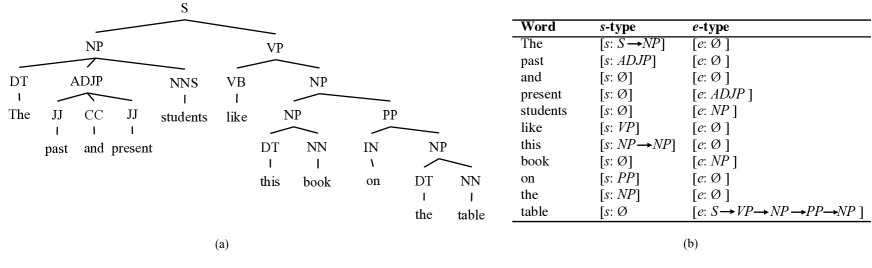
Figure 1: Example constituent hierarchies on the sentence “ The past and present students like this book on the table”. (a) parse tree; (b) constituent hierarchies on words.

Different from that of ?), we collect lookahead constituent information for shift-reduce parsing, rather than pruning information for chart parsing. In addition, our concern is in the accuracies rather than the speed. Accordingly, our model should predict the constituent hierarchy on each word rather than simple boundary information. For example, in Figure 1(a), the constituent hierarchy that the word “The” starts is “S $\rightarrow$ NP”, and the constituent hierarchy that the word “table” ends is “S $\rightarrow$ VP $\rightarrow$ NP $\rightarrow$ PP $\rightarrow$ NP”. For each word, we predict both the constituent hierarchy it starts and the constituent hierarchy it ends, using them as lookahead features.

The task is challenging in three aspects. First, it is significantly more difficult compared to simple sequence labelling, since two sequences of constituent hierarchies must be predicted for each word in the input sequence. Second, for high accuracies, global features from the full sentence are necessary since constituent hierarchies contain rich structural information. Third, to retain high speed for shift-reduce parsing, lookahead feature prediction must be executed efficiently. It is highly difficult to build such a model using manual discrete features and structured search.

Fortunately, sequential recurrent neural networks (RNNs) are remarkably effective models to encode the full input sentence. We leverage RNNs for building our constituent hierarchy predictor. In particular, a LSTM [Hochreiter and Schmidhuber (1997] is used to learn global features automatically from the input words. For each word, a second LSTM is then used to generate the constituent hierarchies greedily using features from the hidden layer of the first LSTM, in the same way as a neural language model decoder generating output sentences for machine translation [Bahdanau et al. (2014]. The resulting model solves all the three challenges raised above. For fully-supervised learning, we learn word embeddings as a part of the model parameters.

In the standard WSJ [Marcus et al. (1993] and CTB 5.1 tests [Xue et al. (2005], our parser gives 1.3 $F_{1}$ and 2.3 $F_{1}$ improvement, respectively, over the baseline of ?), resulting in a accuracy of 91.7 $F_{1}$ for English and 85.5 $F_{1}$ for Chinese, which are the best for fully-supervised models in the literature. We release our code, based on ZPar, at https://github.com/SUTDNLP/LookAheadConparser.

2 Baseline System

We adopt the parser of ?) for a baseline, which is based on the shift-reduce process of ?) and the beam search strategy of ?) with the global perceptron training.

Initial State	$[\phi,0,false,0]$
Final State	$[S,n,true,m:2n<=m<=4n]$
Induction Rules:
Shift	$\frac{[S,i,false,k]}{[S|w,i+1,false,k+1]}$
Reduce-l/r-x	$\frac{[S|s_{1}s_{0},i,false,k]}{[S|X,i,false,k+1]}$
Unary-x	$\frac{[S|s_{0},i,false,k]}{[S|X,i,false,k+1]}$
Finish	$\frac{[S,n,false,k]}{[S,n,true,k+1]}$
Idle	$\frac{[S,n,true,k]}{[S,n,true,k+1]}$

Figure 2: Deduction system for the baseline shift-reduce parsing process.

2.1 The Shift-Reduce System

Shift-reduce parsers process an input sentence incrementally from left to right. A stack is used to maintain partial phrase-structures, while the incoming words are ordered in a buffer. At each step, a transition action is applied to consume an input word or construct a new phrase-structure. The set of transition actions are

• Shift: pop the front word off the buffer, and push it onto the stack.

• Reduce-l/r-x: pop the top two constituents off the stack, combine them into a new constituent with label X, and push the new constituent onto the stack.

• Unary-x: pop the top constituent off the stack, raise it to a new constituent X, and push the new constituent onto the stack.

• Finish: pop the root node off the stack and end parsing.

• Idle: no-effect action on a completed state without changing items on the stack or buffer.

The deduction system for the process is shown in Figure 2, where a state is represented as [stack, buffer front index, completion mark, action index], and $n$ is the number of words in the input. For example, given the sentence “They like apples”, the action sequence “Shift, Shift, Shift, Reduce-L-VP, Reduce-R-S” gives its syntax “(S They (VP like apples) )”.

2.2 Search and Training

Beam-search is used for decoding with the $k$ best state items at each step being kept in the agenda. During initialization, the agenda contains only the initial state [$\phi,0,false,0$]. At each step, each state in the agenda is popped and expanded by applying all valid transition actions, and the top $k$ resulting states are put back onto the agenda [Zhu et al. (2013]. The process repeats until the agenda is empty, and the best completed state is taken as output.

The score of a state is the total score of the transition actions that have been applied to build it:

$$C(\alpha)=\sum^{N}_{i=1}\Phi(\alpha_{i})\cdot\vec{\theta}$$ (1)

Here $\Phi(\alpha_{i})$ represents the feature vector for the $i$th action $\alpha_{i}$ in the state item $\alpha$. $N$ is the total number of actions in $\alpha$.

The model parameter set $\vec{\theta}$ is trained online using the averaged perceptron algorithm with the early-update strategy [Collins and Roark (2004].

Description	Templates
Unigram	$s_{0}tc,s_{0}wc,s_{1}tc,s_{1}wc,s_{2}tc$
	$s_{2}wc,s_{3}tc,s_{3}wc,q_{0}wt,q_{1}wt$
	$q_{2}wt,q_{3}wt,s_{0}lwc,s_{0}rwc$
	$s_{0}uwc,s_{1}lwc,s_{1}rwc,s_{1}uwc$
Bigram	$s_{0}ws_{1}w,s_{0}ws_{1}c,s_{0}cs_{1}w,s_{0}cs_{1}c$
	$s_{0}wq_{0}w,s_{0}wq_{0}t,s_{0}cq_{0}w,s_{0}cq_{0}t$
	$q_{0}wq_{1}w,q_{0}wq_{1}t,q_{0}tq_{1}w,q_{0}tq_{1}t$
	$s_{1}wq_{0}w,s_{1}wq_{0}t,s_{1}cq_{0}w,s_{1}cq_{0}t$
Trigram	$s_{0}cs_{1}cs_{2}c,s_{0}ws_{1}cs_{2}c,s_{0}cs_{1}wq_{0}t$
	$s_{0}cs_{1}cs_{2}w,s_{0}cs_{1}cq_{0}t,s_{0}ws_{1}cq_{0}t$
	$s_{0}cs_{1}wq_{0}t,s_{0}cs_{1}cq_{0}w$
Extended	$s_{0}llwc,s_{0}lrwc,s_{0}luwc$
	$s_{0}rlwc,s_{0}rrwc,s_{0}ruwc$
	$s_{0}ulwc,s_{0}urwc,s_{0}uuwc$
	$s_{1}llwc,s_{1}lrwc,s_{1}luwc$
	$s_{1}rlwc,s_{1}rrwc,s_{1}ruwc$

Table 1: Baseline feature templates, where $s_{i}$ represents the $i$th item on the top of the stack and $q_{i}$ denotes the $i$th item in the front of the buffer. The symbol $w$ denotes the lexical head of an item; the symbol $c$ denotes the constituent label of an item; the symbol $t$ is the POS of a lexical head; $s_{i}ll$ denotes the left child of $s_{i}$’s left child. Other notations can be explained in a similar way.

2.3 Baseline Features

Our baseline features are taken from ?). As shown in Table 1, they include the Unigram, Bigram, Trigram features of ?) and the extended features of ?).

3 Global Lookahead Features

The baseline features suffer two limitations, as mentioned in the introduction. First, they are relatively local to the state, considering only the neighbouring nodes of $s_{0}$ (top of stack) and $q_{0}$ (front of buffer). Second, they do not consider lookahead information beyond $s_{3}$, or the syntactic structure of the buffer and sequence. We use a LSTM to capture full sentential information in linear time, representing such global information into the baseline parser as a constituent hierarchy for each word. Lookahead features are extracted from the constituent hierarchy to provide top-down guidance for bottom-up parsing.

Templates
$s_{0}c_{g}s,s_{0}c_{g}e,s_{1}c_{g}s,s_{1}c_{g}e$
$q_{0}c_{g}s,q_{0}c_{g}e,q_{1}c_{g}s,q_{1}c_{g}e$

Table 2: Lookahead feature templates, where $s_{i}$ represents the $i$th item on the top of the stack and $q_{i}$ denotes the $i$th item in the front end of the buffer. The symbol $c_{g}s$ and $c_{g}e$ denote the next level constituent in the $s$-type hierarchy and $e$-type hierarchy, respectively.

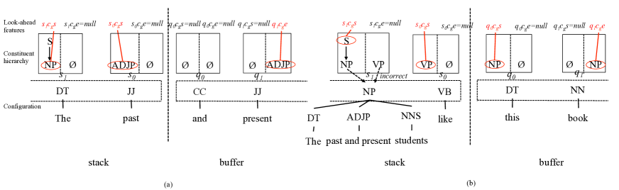
Figure 3: Two intermediate states of parsing on the sentence “The past and present students like this book on the table”. Each item on the stack or buffer has two constituent hierarchies: s-type (left) and e-type (right), respectively, in the corresponding box. Noted that the e-type constituent hierarchy of the word “students” are incorrectly predicted and used as soft features in our model.

3.1 Constituent Hierarchy

In a constituency tree, each word can start or end a constituent hierarchy. As shown in Figure 1, the word “The” starts a constituent hierarchy “S $\rightarrow$ NP”. In particular, it starts a constituent S in the top level and then a following constituent NP. The word “table” ends a constituent hierarchy “S $\rightarrow$ VP $\rightarrow$ NP $\rightarrow$ PP $\rightarrow$ NP”. In particular, it ends a constituent S in the top level, and then a VP (starting from the word “like”), an NP (starting from the noun phrase “this book”), a PP (starting from the word “in”), and finally an NP (starting from the word “the”). The extraction of constituent hierarchies for each word is based on unbinarized grammars, reflecting the start and end in unbinarized trees. The constituent hierarchy is empty (denoted as $\phi$) if the corresponding words does not start or end a constituent. The constituent hierarchies are added into the shift-reduce parser as soft features (section 3.2).

Formally, a constituent hierarchy is defined as

$$[type:c_{1}\rightarrow c_{2}\rightarrow...\rightarrow c_{z}],$$

where $c$ is a constituent label (e.g. NP), “$\rightarrow$” represents the top-down hierarchy, and $type$ can be $s$ or $e$, denoting that the current word starts or ends the constituent hierarchy, respectively, as shown in Figure 1. Compared with full parsing, the constituent hierarchies associated with each word have no forced structural dependencies between each other, and therefore can be modelled more easily, for each word individually. Serving as soft lookahead features rather than hard constraints, their inter-dependencies are not crucial for the main parser.

3.2 Lookahead Features

The lookahead feature templates are defined in Table 2. In order to ensure parsing efficiency, only simple feature templates are taken into consideration. The lookahead features of a state are instantiated for the top two items on the stack (i.e. $s_{0}$ and $s_{1}$) and buffer (i.e. $q_{0}$ and $q_{1}$). The new function $\Phi^{\prime}$ is defined to output the lookahead features vector. The score of a state in our model is simple extended form the Formula (1):

$$C(\alpha)=\sum^{N}_{i=1}\Phi(\alpha_{i})\cdot\vec{\theta}+\Phi^{\prime}(\alpha_{i})\cdot\vec{\theta^{\prime}}$$

For each word, the lookahead feature represents the next level constituent in the top-down hierarchy, which can guide bottom-up parsing.

For example, Figure 3 shows two intermediate states during parsing. In Figure 3(a), the $s$-type and $e$-type lookahead features of $s_{1}$ (i.e. the word “The”) are extracted from the constituent hierarchy in the bottom level, namely NP and Null, respectively. On the other hand, in Figure 3(b), The $s$-type lookahead feature of $s_{1}$ is extracted from the $s$-type constituent hierarchy of same word “The”, but is S based on current hierarchical level. The $e$-type lookahead feature, on the other hand, is extracted from the $e$-type constituent hierarchy of end word “students” of the VP constituent, which is Null in the next level. Lookahead features for items on the buffer are extracted in the same way.

The lookahead features are useful for guiding shift-reduce decisions given the current state. For example, given the intermediate state in Figure 3(a), $s_{0}$ has a $s$-type lookahead feature ADJP, and $q_{1}$ in the buffer has $e$-type lookahead feature ADJP. This indicates that the two items are likely reduced into the same constituent. Further, $s_{0}$ cannot end a constituent because of the empty $e$-type constituent hierarchy. As a result, the final shift-reduce parser will assign more possibility to Shift decision.

4 Constituent Hierarchy Prediction

We propose a novel neural model for constituent hierarchy prediction. Inspired by the encoder-decoder framework for neural machine translation [Bahdanau et al. (2014, Cho et al. (2014], we use a LSTM to capture full sentence features, and another LSTM to generate the constituent hierarchies for each word. Compared with a CRF-based sequence labelling model [Roark and Hollingshead (2009], the proposed model has three advantages. First, the global features can be automatically represented. Second, it can avoid the exponentially large number of labels if constituent hierarchies are treated as unique labels. Third, the model size is relatively small, and does not have a large effect on the final parser model.

As shown in Figure 4, the neural network consists of three main layers, namely the input layer, the encoder layer and the decoder layer. The input layer represents each word using its characters and token information; the encoder hidden layer uses a bidirectional recurrent neural network structure to learn global features from the sentence; and the decoder layer predicts constituent hierarchies according to the encoder layer features, by using attention mechanism [Bahdanau et al. (2014] to softly compute the contribution of each hidden unit of the encoder.

4.1 Input Layer

The input layer generates a dense vector representation of each input word. We use character embeddings to alleviate OOV problems in word embeddings [Ballesteros et al. (2015, Santos and Zadrozny (2014, Kim et al. (2016], concatenating a character-embedding representation of a word to its word embedding. Formally, the input representation $x_{i}$ of the word $w_{i}$ is computed by:

$$\begin{split}x_{i}&=x_{w_{i}}\oplus c_{i\_att}\\ c_{i\_att}&=\sum_{j}\alpha_{ij}c_{ij},\end{split}$$

where $x_{w_{i}}$ is a word embedding vector of the word $w_{i}$ according to a embedding lookup table, $c_{i\_att}$ is a character embedding form of the word $w_{i}$, $c_{ij}$ is the $j$th character in $w_{i}$, and $\alpha_{ij}$ is the contribution of the character $c_{ij}$ to $c_{i\_att}$, which is computed by:

$$\begin{split}\alpha_{ij}&=\frac{e^{f(x_{w_{i}},c_{ij})}}{\sum_{k}e^{f(x_{w_{i}},c_{ik})}}\end{split}$$

$f$ is a non-linear transformation function based on tanh function.

4.2 Encoder Layer

The encoder first uses a window strategy to represent input nodes with their corresponding local context nodes. Formally, a windowed word representation takes the form

$$\begin{split}x^{\prime}_{i}&=[x_{i-win};...;x_{i};...;x_{i+win}].\\ \end{split}$$

Second, the encoder scans the input sentence and generates hidden units for each input word using a recurrent neural network (RNN), which represents features of the word from the global sequence. Formally, given the windowed input nodes $x^{\prime}_{1}$, $x^{\prime}_{2}$, …, $x^{\prime}_{n}$ for the sentence $w_{1}$, $w_{2}$, …, $w_{n}$, the RNN layer calculates a hidden node sequence $h_{1}$, $h_{2}$, …, $h_{n}$.

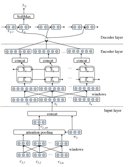
Figure 4: Structure of the constituent hierarchy prediction model. $c_{ij}$ denotes the $j$th character of the word $w_{i}$; $\overrightarrow{h_{i}}$ denotes the left-to-right encoder hidden units; $\overleftarrow{h_{i}}$ denotes the right-to-left encoder hidden units; $s$ denotes the decoder hidden unit; and $y_{ij}$ is the $j$th label of the word $w_{i}$.

Long Short-Term Memory (LSTM) mitigates the vanishing gradient problem in RNN training, by introducing gates (i.e. input $i$, forget $f$ and output $o$) and a cell memory vector $c$. We use the variation of ?). Formally, the values in the LSTM hidden layers are computed as follows:

$$\begin{split}i_{i}&=\sigma(W_{1}x^{\prime}_{i}+W_{2}h_{i-1}+W_{3}\odot c_{i-1}+b_{1})\\ f_{i}&=1-i_{i}\\ \tilde{c}_{i}&=tanh(W_{4}x^{\prime}_{i}+W_{5}h_{i-1}+b_{2})\\ c_{i}&=f_{i}\odot c_{i-1}+i_{i}\odot\tilde{c}_{i}\\ o_{i}&=\sigma(W_{6}x^{\prime}_{i}+W_{7}h_{i-1}+W_{8}\odot c_{i}+b_{3})\\ h_{i}&=o_{i}\odot tanh(c_{i}),\end{split}$$

where $\odot$ is pair-wise multiplication. Further, in order to collect features for $x_{i}$ from both $x^{\prime}_{1}$, .., $x^{\prime}_{i-1}$ and $x^{\prime}_{i+1}$, … $x^{\prime}_{n}$, we use a bidirectional variation [Schuster and Paliwal (1997, Graves et al. (2013]. As shown in Figure 4, the hidden units are generated by concatenating the corresponding hidden layers of a left-to-right LSTM $\overrightarrow{h_{i}}$ and a right-to-left LSTM $\overleftarrow{h_{i}}$, where $h_{i}=\overrightarrow{h_{i}}\oplus\overleftarrow{h_{i}}$ for each word $w_{i}$.

4.3 Decoder Layer

The decoder hidden layer uses two different LSTMs to generate the $s$-type and $e$-type sequences of constituent labels from each encoder hidden output, respectively, as shown in Figure 4. Each constituent hierarchy is generated bottom-up recurrently. In particular, a sequence of state vectors is generated recurrently, with each state yielding a output constituent label. The process starts with a $\vec{0}$ state vector and ends when a Null constituent is generated. The recurrent state transition process is achieved using LSTM model with the hidden vectors of the encoder layer being used for context features.

Formally, for the word $w_{i}$, the value of the $j$th state unit $s_{ij}$ of the LSTM is computed by:

$$s_{ij}=f(s_{ij-1},c_{ij},h_{i}),$$

where the context $c_{ij}$ is computed by:

$$\begin{split}c_{ij}&=\sum_{k}\beta_{ijk}h_{k}\\ \beta_{ijk}&=\frac{e^{f(s_{ij-1},h_{k})}}{\sum_{k^{\prime}}e^{f(s_{ij-1},h_{k^{\prime}})}}\end{split}$$

Here $h_{k}$ refers to the encoder hidden vector for $w_{k}$. The weight of contribution $\beta_{ijk}$ are computed under attention mechanism [Bahdanau et al. (2014]. The start state $s_{i,-1}=\vec{0}$.

The constituent labels are generated from each state unit $s_{ij}$, where each constituent label $y_{ij}$ is the output of a SoftMax function.

$$p(y_{ij}=l)=\frac{e^{s_{ij}^{\top}W_{l}}}{\sum_{k}e^{s_{ij}^{\top}W_{k}}}$$

$y_{ij}=l$ denotes that the $j$th label of the $i$th word is $l(l\in L$).

As shown in Figure 4, the SoftMax functions are applied to the state units of the decoder, generating hierarchical labels bottom-up, until the default label Null is predicted.

4.4 Training

We use two separate models to assign the $s$-type and $e$-type labels, respectively. For training each constituent hierarchy predictor, we minimize the following training objective:

$$\begin{split}L(\theta)&=-\sum_{i}^{T}\sum_{j}^{Z_{i}}log~{}p_{ijo}+\frac{\lambda}{2}||\theta||^{2},\\ \end{split}$$

where $T$ is the the size of the sentence, $Z_{i}$ is the depth of the constituent hierarchy of the word $w_{i}$, and $p_{ijo}$ stands for $p(y_{ij}=o)$, which is given by the SoftMax function, and $o$ is the golden label.

We apply back-propagation, using momentum stochastic gradient descent [Sutskever et al. (2013] with a learning rate of $\eta=0.01$ for optimization and regularization parameter $\lambda=10^{-6}$.

5 Experiments

5.1 Experiment Settings

English data come from the Wall Street Journal (WSJ) corpus of the Penn Treebank [Marcus et al. (1993]. We use sections 2-21 for training, section 24 for system development, and section 23 for final performance evaluation. Chinese data come from the version 5.1 of the Penn Chinese Treebank (CTB) [Xue et al. (2005]. We use articles 001- 270 and 440-1151 for training, articles 301-325 for system development, and articles 271-300 were used for final performance evaluation. For both English and Chinese data, we adopt ZPar for POS tagging, and use ten-fold jackknifing to assign auto POS tags to the training data. In addition, we use ten-fold jackknifing to assign auto constituent hierarchies to the training data.

We use $F_{1}$ score to evaluate the constituent hierarchy prediction. For example, the constituent prediction is “S $\rightarrow$ S $\rightarrow$ VP $\rightarrow$ NP” and the golden is “S $\rightarrow$ NP $\rightarrow$ NP”. The evaluation starts from the bottom to the top, and the precision is 2/4 = 0.5, the recall is 2/3 = 0.66 and the $F1$ score is 0.57. The metric evaluates the precision and recall of each label in the constituent hierarchy. A label is counted as correct if and only if it occurs in the correct position index. We use Evalb to evaluate parsing performance, including labelled precision ($LP$), labelled recall ($LR$), and bracketing $F_{1}$.

5.2 Model Settings

For training the constituent hierarchy prediction model, gold constituent labels are derived from labelled constituency trees in the training data. The hyper-parameters are chosen according to development tests, and the values are shown in Table 3.

hyper-parameters	value
Word embedding size	50
Word windows	2
Character embedding size	30
Character windows	2
LSTM hidden layer size	100
Character hidden layer size	60

Table 3: Hyper-parameter settings

	$s$-type	$e$-type	parser
1-layer	93.39	81.50	90.43
2-layer	93.76	83.37	90.72
3-layer	93.84	83.42	90.80

Table 4: Performance of the constituent hierarchy predictor and the corresponding parser on the WSJ dev dataset. $n$-layer denotes a LSTM model with $n$ hidden layers.

	$s$-type	$e$-type	parser
all	93.76	83.37	90.72
all w/o wins	93.62	83.34	90.58
all w/o chars	93.51	83.21	90.33
all w/o chars & wins	93.12	82.36	89.18

Table 5: Performance of the constituent hierarchy predictor and the corresponding parser on the WSJ dev dataset. all denotes the proposed model without ablation.

For the shift-reduce constituency parser, we set the beam size to 16 for both training and decoding, which achieves a good tradeoff between efficiency and accuracy [Zhu et al. (2013]. The optimal training iteration number is determined on the development sets.

5.3 Results of Constituent Hierarchy Prediction

Table 4 shows the results of constituent hierarchy prediction, where word and character embeddings are randomly initialized, and fine-tuned during training. The third column shows the development parsing accuracies when the labels are used for lookahead features. As Table 4 shows, when the number of hidden layer increase, both $s$-type and $e$-type constituent hierarchy prediction improve. The accuracies of $e$-type prediction is relatively lower due to right-branching in the treebank, which makes $e$-type hierarchies longer than $s$-type hierarchies. In addition, a 3-layer LSTM does not give significantly improvements compared to 2-layer LSTM. For tradeoff between efficiency and accuracy, we choose the 2-layer LSTM as our constituent hierarchy predictor.

Table 5 shows ablation results of constituent hierarchy prediction given by different reduced architectures, which include an architecture without character embeddings and an architecture with neither character embeddings nor input windows. We find that the original architecture achieves the highest performance on constituent hierarchy prediction, compared to the two baselines. The baseline only without the character embeddings has relatively small influence on constituent hierarchy prediction. On the other hand, the baseline only without the input word windows has relatively smaller influence on constituent hierarchy prediction. Nevertheless, both of these two ablation architectures lead to much lower parsing accuracies. The baseline removing both the character embeddings and the input word windows has relatively low accuracies.

Parser	LR	LP	F1
Fully-supervised
?)	86.3	87.5	86.9
?)	89.5	89.9	89.5
?)	88.1	88.3	88.2
?)$\dagger$	86.1	86.0	86.0
?)$\dagger$	87.8	88.1	87.9
?)	90.1	90.2	90.1
?)	90.7	91.4	91.1
?)	N/A	N/A	91.1
?)$\dagger$	90.2	90.7	90.4
?)*	N/A	N/A	90.4
?)*	N/A	N/A	88.3
This work	91.3	92.1	91.7
Ensemble
?)	N/A	N/A	92.4
?)*	N/A	N/A	90.5
Rerank
?)	91.2	91.8	91.5
?)	92.2	91.2	91.7
Semi-supervised
?)	92.1	92.5	92.3
?)	91.1	91.6	91.3
?)	91.4	91.8	91.6
?)$\dagger$	91.1	91.5	91.3
?)*	N/A	N/A	91.1
?)*$\dagger$	N/A	N/A	92.4

Table 6: Comparison of related work on the WSJ test set. * denotes neural parsing; $\dagger$ denotes shift-reduce framework.

Parser	LR	LP	F1
Fully-supervised
?)	79.6	82.1	80.8
?)	79.3	82.0	80.6
?)	81.9	84.8	83.3
?)$\dagger$	82.1	84.3	83.2
?)$\ddagger$	N/A	N/A	83.2
This work	85.2	85.9	85.5
Rerank
?)	80.8	83.8	82.3
Semi-supervised
?)$\dagger$	84.4	86.8	85.6
Wand and Xue [Wang and Xue (2014]$\ddagger$	N/A	N/A	86.3
Wang et al. [Wang et al. (2015]$\ddagger$	N/A	N/A	86.6
Dyer et al. [Dyer et al. (2016]*$\dagger$	N/A	N/A	82.7

Table 7: Comparison of related work on the CTB5.1 test set. * denotes neural parsing; $\dagger$ denotes shift-reduce framework; $\ddagger$ denotes joint POS tagging and parsing.

5.4 Final Results

For English, we compare the final results with previous related work on the WSJ test sets. As shown in Table 6, our model achieves 1.3% $F_{1}$ improvement compared to the baseline parser with fully-supervised learning [Zhu et al. (2013]. Our model outperforms the state-of-the-art fully-supervised system [Carreras et al. (2008, Shindo et al. (2012] by 0.6% $F_{1}$. In addition, our fully-supervised model also catches up with many state-of-the-art semi-supervised models [Zhu et al. (2013, Huang and Harper (2009, Huang et al. (2010, Durrett and Klein (2015] by achieving 91.7% $F_{1}$ on WSJ test set. The size of our model is much smaller than the semi-supervised model of Zhu et al. [Zhu et al. (2013], which contains rich features from a large automatically parsed corpus. In contrast, our model is about the same in size compared to the baseline parser.

We carry out Chinese experiments with the same models, and compare the final results with previous related work on the CTB test set. As shown in Table 7, our model achieves 2.3% $F_{1}$ improvement compared to the state-of-the-art baseline system with fully-supervised learning [Zhu et al. (2013], which are by far the best results in the literature. In addition, our fully-supervised model is also comparable to many state-of-the-art semi-supervised models [Zhu et al. (2013, Wang and Xue (2014, Wang et al. (2015, Dyer et al. (2016] by achieving 85.5% $F_{1}$ on the CTB test set. ?) and ?) do joint POS tagging and parsing.

5.5 Comparison of Speed

Table 8 shows the running times of various parsers on test sets on a Intel 2.2 GHz processor with 16G memory. Our parsers are much faster than the related parser with the same shift-reduce framework [Sagae and Lavie (2005, Sagae and Lavie (2006]. Compared to the baseline parser, our parser gives significant improvement on accuracies (90.4% to 91.7% $F_{1}$) at the speed of 79.2 sentences per second, in contrast to 89.5 sentences per second on the standard WSJ benchmark.

Parser	#Sent/Second
Ratnaparkhi [Ratnaparkhi (1997]	Unk
Collins [Collins (2003]	3.5
Charniak [Charniak (2000]	5.7
Sagae and Lavie [Sagae and Lavie (2005]	3.7
Sagae and Lavie [Sagae and Lavie (2006]	2.2
Petrov and Klein [Petrov and Klein (2007]	6.2
Carreras et al. [Carreras et al. (2008]	Unk
Zhu et al. [Zhu et al. (2013]	89.5
This work	79.2

Table 8: Comparison of running times on the test set, where the time for loading models is excluded. The running times of related parsers are taken from Zhu et al. [Zhu et al. (2013].

6 Errors Analysis

We conduct error analysis by measuring: parsing accuracies against different phrase types, constituents of different span lengths, and different sentence lengths.

6.1 Phrase Type

Table 9 shows the accuracies of the baseline and the final parsers with lookahead features on 9 common phrase types. As the results show, while the parser with lookahead features achieves improvements on all of the frequent phrase types, there are relatively more improvements on constituent VP, S, SBAR and WHNP.

The constituent hierarchy predictor has relatively better performance on $s$-type labels for the constituents VP and WHNP, which are prone to errors by the baseline system. The constituent hierarchy can give guidance to the constituent parser for tackling the challenges. Compared to the $s$-type constituent hierarchy, the $e$-type constituent hierarchy is relatively more difficult to predict, particularly for the constituents with long spans such as VP, S and SBAR. Despite this, the $e$-type constituent hierarchies with relatively low accuracies also benefit prediction of constituents with long spans.

		NP	VP	S	PP	SBAR	ADVP	ADJP	WHNP	QP
baseline		92.06	90.63	90.28	87.93	86.93	84.83	74.12	95.03	89.32
with lookahead feature		93.10	92.45	91.78	88.84	88.59	85.64	74.50	96.18	89.63
improvement		+1.04	+1.82	+1.50	+0.91	+1.66	+0.81	+0.38	+1.15	+0.31
constituent hierarchy	$s$-type	95.18	97.51	93.37	98.01	92.14	88.94	79.88	96.18	91.70
	$e$-type	91.98	76.82	80.72	84.80	66.82	85.01	71.16	95.13	91.02

Table 9: Comparison between the parsers with lookahead features on different phrases types, with the corresponding constituent hierarchy predictor performances.

6.2 Span Length

Figure 5 shows comparison of the two parsers on constituents with different span lengths. As the results show, lookahead features are helpful on both large spans and small spans, while the performance gap between the two parsers is larger as the size of span increases. This reflects the usefulness of long-range information captured by the constituent hierarchy predictor and lookahead features.

Figure 5: Comparison with the baseline on spans of different lengths.

6.3 Sentence Length

Figure 6 shows comparison of the two parsers on sentences of different lengths. As the results show, the parser with lookahead features outperforms the baseline system on both short sentences and long sentences. Also, the performance gap between the two parsers is larger as the length of sentence increases.

The constituent hierarchy predictors generate hierarchical constituents for each input word using global information. For longer sentences, the predictors yield deeper constituent hierarchies, offering corresponding lookahead features. As a result, compared to the baseline parser, the performance of the parser with lookahead features decreases more slowly as the length of the sentences increases.

Figure 6: Comparison with the baseline on sentences of different lengths. Sentences with length [0, 10) fall in the bin 10.

7 Related Work

Our lookahead features are similar in spirit to the pruners of Roark and Hollingshead [Roark and Hollingshead (2009] and Zhang et al. [Zhang et al. (2010b], which infer the maximum length of constituents that a particular word can start or end. However, our method is different in three main perspectives. First, rather than using a CRF with sparse local word window features, a neural network is used for dense global features on the sentence. Second, not only the size of constituents but also the constituent hierarchy is identified for each word. Third, the results are added into a transition-based parser as soft features, rather then being used as hard constraints to a chart parser.

Our concepts of constituent hierarchies are similar with the work of supertagging. For lexicalized grammars such as Combinatory Categorial Grammar (CCG), Tree-Adjoining Grammar (TAG) and Head-Driven Phrase Structure Grammar (HPSG), each word in the input sentence is assigned one or more super tags, which are used to identify the syntactic role of the word for constraint parsing [Clark (2002, Clark and Curran (2004, Carreras et al. (2008, Ninomiya et al. (2006, Dridan et al. (2008]. For a lexicalized grammar, supertagging can benefit the parsing in both accuracy and efficiency by offering almost-parsing information. In particular, ?) defined the concept spine in TAG, which is similar to our constituent hierarchy. However, there are three differences. First, the spine is defined to describe the main syntactic tree structure with a series of unary projections, while constituent hierarchy is defined to describe how words can start or end hierarchical constituents (it is possible to be empty if the word cannot start or end constituents). Second, spines are extracted from gold trees and used to prune the search space of parsing as hard constraints. In contrast, we use constituent hierarchies as soft features. Third, ?) use spines to prune a chart parsing, while we use constituent hierarchies to improve a linear shift-reduce parser.

Under the lexicalized grammar, this supertagging can benefit the parsing with more accuracy and efficiency as almost parsing [Bangalore and Joshi (1999]. Recently, the works on obtaining the super tags appear. ?) proposed the efficient methods to obtain super tags for HPSG parsing using dependency information. ?) and ?) turn to design recursive neural network for supertagging for CCG parsing. In contrast, our models predict the constituent hierarchy instead of single super tag for each word in the input sentence, which are also likely regarded as the member of multiple ordered labels prediction family.

Our constituent hierarchy predictor is also related to sequence-to-sequence learning [Sutskever et al. (2014], which is successful in neural machine translation [Bahdanau et al. (2014]. The neural model encodes the source-side sentence into dense vectors, and then uses them to generate target-side word by word. There has also been work that directly use sequence-to-sequence model for constituent parsing, which generates bracketed constituency tree given raw sentences [Vinyals et al. (2015, Luong et al. (2015]. Compared to Vinyals et al. [Vinyals et al. (2015], who predicts a full parser tree from input, our predictors tackle a much simpler task, by predicting the constituent hierarchies of each word separately. In addition, the outputs of the predictors are used for soft lookahead features in bottom-up parsing, rather than being taken as output structures directly.

By integrating the neural constituent hierarchy predictor, our parser is related to neural network models for parsing, which has given competitive accuracies for both constituency parsing [Dyer et al. (2016, Watanabe and Sumita (2015] and dependency parsing [Chen and Manning (2014, Zhou et al. (2015, Dyer et al. (2015]. In particular, our parser is more closely related to neural models that integrates discrete manual features [Socher et al. (2013, Durrett and Klein (2015]. Soccer et al. use neural features to rerank a sparse baseline parser; Durrett and Klein directly integrate sparse features into neural layers in a chart parser. In contrast, we integrate neural information into sparse features in the form of lookahead features.

There has also been work on lookahead features for parsing. Tsuruoka et al. [Tsuruoka et al. (2011] run a baseline parser for a few future steps, and use the output actions to guide the current action. In contrast to their model, our model leverages full sentential information, yet is significantly faster.

Existing work on investigated efficiency of parsing without loss of accuracy, which is required by real time applications, such as web parser, processing massive amounts of textual data. ?) introduced a chart pruner to accelerate a CCG parser. ?) proposed novel self-training method focusing on increasing the speed of a CCG parser rather than its accuracy.

8 Conclusion

We proposed a novel constituent hierarchy predictor based on recurrent neural networks, aiming to capture global sentential information. The resulting constituent hierarchies are fed to a baseline shift-reduce parser as lookahead features, addressing the limitation of shift-reduce parsers in not leveraging right-hand side syntax for local decisions, yet maintaining the same model size and speed. The resulting fully-supervised parser outperforms the state-of-the-art baseline parser by achieving 91.7% $F_{1}$ on standard WSJ evaluation and 85.5% $F_{1}$ on standard CTB evaluation.

References

- [Bahdanau et al. (2014] Dzmitry Bahdanau, Kyunghyun Cho, and Yoshua Bengio. 2014. Neural Machine Translation by Jointly Learning to Align and Translate. CoRR.
- [Ballesteros et al. (2015] Miguel Ballesteros, Chris Dyer, and Noah A Smith. 2015. Improved Transition-Based Parsing by Modeling Characters instead of Words with LSTMs. In EMNLP, pages 349–359.
- [Bangalore and Joshi (1999] Srinivas Bangalore and Aravind K Joshi. 1999. Supertagging: an approach to almost parsing. Computational Linguistics, 25(2):237–265, June.
- [Bikel (2004] Daniel M Bikel. 2004. On the parameter space of generative lexicalized statistical parsing models. In Ph.D Thesis, University of Pennsylvania.
- [Carreras et al. (2008] Xavier Carreras, Michael Collins, and Terry Koo. 2008. TAG, dynamic programming, and the perceptron for efficient, feature-rich parsing. In CoNLL, pages 9–16, Morristown, NJ, USA. Association for Computational Linguistics.
- [Charniak and Johnson (2005] Eugene Charniak and Mark Johnson. 2005. Coarse-to-Fine n-Best Parsing and MaxEnt Discriminative Reranking. In ACL.
- [Charniak (2000] Eugene Charniak. 2000. A Maximum-Entropy-Inspired Parser. In ANLP, pages 132–139.
- [Chen and Manning (2014] Danqi Chen and Christopher Manning. 2014. A Fast and Accurate Dependency Parser using Neural Networks. In EMNLP, pages 740–750, Stroudsburg, PA, USA. Association for Computational Linguistics.
- [Cho et al. (2014] Kyunghyun Cho, Bart van Merrienboer, Çaglar Gülçehre, Dzmitry Bahdanau, Fethi Bougares, Holger Schwenk, and Yoshua Bengio. 2014. Learning Phrase Representations using RNN Encoder-Decoder for Statistical Machine Translation. In EMNLP, pages 1724–1734.
- [Clark and Curran (2004] Stephen Clark and James R Curran. 2004. The importance of supertagging for wide-coverage CCG parsing. In COLING, pages 282–288, Morristown, NJ, USA, August. University of Edinburgh, Association for Computational Linguistics.
- [Clark (2002] Stephen Clark. 2002. Supertagging for combinatory categorial grammar. In Proceedings of the Sixth International Workshop on Tree Adjoining Grammar and Related Frameworks, pages 101–106, Universita di Venezia.
- [Collins and Roark (2004] Michael Collins and Brian Roark. 2004. Incremental parsing with the perceptron algorithm. In ACL, pages 111–es, Morristown, NJ, USA. Association for Computational Linguistics.
- [Collins (2003] Michael Collins. 2003. Head-driven statistical models for natural language parsing. Computational linguistics, 29(4):589–637.
- [Dridan et al. (2008] R Dridan, V Kordoni, and J Nicholson. 2008. Enhancing Performance of Lexicalised Grammars. In ACL.
- [Durrett and Klein (2015] Greg Durrett and Dan Klein. 2015. Neural CRF Parsing. In ACL, pages 302–312.
- [Dyer et al. (2015] Chris Dyer, Miguel Ballesteros, Wang Ling, Austin Matthews, and Noah A Smith. 2015. Transition-Based Dependency Parsing with Stack Long Short-Term Memory. In ACL-IJCNLP, pages 334–343.
- [Dyer et al. (2016] Chris Dyer, Adhiguna Kuncoro, Miguel Ballesteros, and Noah A Smith. 2016. Recurrent Neural Network Grammars. In NAACL, pages 199 – 209.
- [Goodman (1998] Joshua Goodman. 1998. Parsing Inside-Out. In PhD thesis.
- [Graves and Schmidhuber (2008] Alex Graves and Jürgen Schmidhuber. 2008. Offline Handwriting Recognition with Multidimensional Recurrent Neural Networks. In NIPS, pages 545–552.
- [Graves et al. (2013] Alex Graves, Navdeep Jaitly, and Abdel-rahman Mohamed. 2013. Hybrid speech recognition with Deep Bidirectional LSTM. In IEEE Workshop on Automatic Speech Recognition & Understanding (ASRU), pages 273–278. IEEE.
- [Hochreiter and Schmidhuber (1997] Sepp Hochreiter and Jürgen Schmidhuber. 1997. Long Short-Term Memory. Neural Computation, 9(8):1735–1780, November.
- [Huang and Harper (2009] Zhongqiang Huang and Mary P Harper. 2009. Self-Training PCFG Grammars with Latent Annotations Across Languages. In EMNLP, pages 832–841.
- [Huang et al. (2010] Zhongqiang Huang, Mary P Harper, and Slav Petrov. 2010. Self-Training with Products of Latent Variable Grammars. In EMNLP, pages 12–22.
- [Huang (2008] Liang Huang. 2008. Forest Reranking: Discriminative Parsing with Non-Local Features. In ACL, pages 586–594.
- [Kim et al. (2016] Yoon Kim, Yacine Jernite, David Sontag, and Alexander M Rush. 2016. Character-Aware Neural Language Models. In AAAI.
- [Kummerfeld et al. (2010] Jonathan K Kummerfeld, Jessika Roesner, Tim Dawborn, James Haggerty, James R Curran, and Stephen Clark. 2010. Faster parsing by supertagger adaptation. In ACL, pages 345–355. University of Cambridge, Association for Computational Linguistics, July.
- [Luong et al. (2015] Minh-Thang Luong, Quoc V Le, Ilya Sutskever, Oriol Vinyals, and Lukasz Kaiser. 2015. Multi-task Sequence to Sequence Learning. ICLR.
- [Marcus et al. (1993] Mitchell P Marcus, Beatrice Santorini, and Mary Ann Marcinkiewicz. 1993. Building a Large Annotated Corpus of English: The Penn Treebank. Computational Linguistics, 19(2):313–330.
- [McClosky et al. (2006] David McClosky, Eugene Charniak, and Mark Johnson. 2006. Effective self-training for parsing. In HLT-NAACL, pages 152–159, Morristown, NJ, USA. Association for Computational Linguistics.
- [Ninomiya et al. (2006] Takashi Ninomiya, Takuya Matsuzaki, Yoshimasa Tsuruoka, Yusuke Miyao, and Jun’ichi Tsujii. 2006. Extremely lexicalized models for accurate and fast HPSG parsing. In EMNLP, pages 155–163. University of Manchester, Association for Computational Linguistics, July.
- [Petrov and Klein (2007] Slav Petrov and Dan Klein. 2007. Improved Inference for Unlexicalized Parsing. In HLT-NAACL, pages 404–411.
- [Ratnaparkhi (1997] Adwait Ratnaparkhi. 1997. A Linear Observed Time Statistical Parser Based on Maximum Entropy Models. In EMNLP.
- [Roark and Hollingshead (2009] Brian Roark and Kristy Hollingshead. 2009. Linear Complexity Context-Free Parsing Pipelines via Chart Constraints. In HLT-NAACL, pages 647–655.
- [Sagae and Lavie (2005] Kenji Sagae and Alon Lavie. 2005. A classifier-based parser with linear run-time complexity. In IWPT, pages 125–132, Morristown, NJ, USA. Association for Computational Linguistics.
- [Sagae and Lavie (2006] Kenji Sagae and Alon Lavie. 2006. Parser combination by reparsing. In HLT-NAACL, pages 129–132, Morristown, NJ, USA. Association for Computational Linguistics.
- [Santos and Zadrozny (2014] Cicero D Santos and Bianca Zadrozny. 2014. Learning character-level representations for part-of-speech tagging. In ICML, pages 1818–1826.
- [Schuster and Paliwal (1997] Mike Schuster and Kuldip K Paliwal. 1997. Bidirectional recurrent neural networks. Signal Processing, IEEE transaction, 45(11):2673–2681.
- [Shindo et al. (2012] Hiroyuki Shindo, Yusuke Miyao, Akinori Fujino, and Masaaki Nagata. 2012. Bayesian Symbol-Refined Tree Substitution Grammars for Syntactic Parsing. In ACL, pages 440–448.
- [Socher et al. (2013] Richard Socher, John Bauer, Christopher D Manning, and Andrew Y Ng. 2013. Parsing with Compositional Vector Grammars. In ACL, pages 455–465.
- [Sutskever et al. (2013] Ilya Sutskever, James Martens, George E Dahl, and Geoffrey E Hinton. 2013. On the importance of initialization and momentum in deep learning. In ICML, pages 1139–1147.
- [Sutskever et al. (2014] Ilya Sutskever, Oriol Vinyals, and Quoc V Le. 2014. Sequence to Sequence Learning with Neural Networks. In NIPS, pages 3104–3112.
- [Tsuruoka et al. (2011] Yoshimasa Tsuruoka, Yusuke Miyao, and Jun’ichi Kazama. 2011. Learning with Lookahead: Can History-Based Models Rival Globally Optimized Models? In CoNLL, pages 238–246.
- [Vaswani et al. (2016] A Vaswani, Y Bisk, and K Sagae. 2016. Supertagging with LSTMs. In NAACL.
- [Vinyals et al. (2015] Oriol Vinyals, Lukasz Kaiser, Terry Koo, Slav Petrov, Ilya Sutskever, and Geoffrey E Hinton. 2015. Grammar as a Foreign Language. In NIPS, pages 2773–2781.
- [Wang and Xue (2014] Zhiguo Wang and Nianwen Xue. 2014. Joint POS Tagging and Transition-based Constituent Parsing in Chinese with Non-local Features. In ACL, pages 733–742, Stroudsburg, PA, USA. Association for Computational Linguistics.
- [Wang et al. (2015] Zhiguo Wang, Haitao Mi, and Nianwen Xue. 2015. Feature Optimization for Constituent Parsing via Neural Networks. In ACL-IJCNLP, pages 1138–1147, Stroudsburg, PA, USA. Association for Computational Linguistics.
- [Watanabe and Sumita (2015] Taro Watanabe and Eiichiro Sumita. 2015. Transition-based Neural Constituent Parsing. In ACL, pages 1169–1179.
- [Xu et al. (2015] Wenduan Xu, Michael Auli, and Stephen Clark. 2015. CCG Supertagging with a Recurrent Neural Network. In ACL-IJCNLP, pages 250–255, Stroudsburg, PA, USA. Association for Computational Linguistics.
- [Xue et al. (2005] Naiwen Xue, Fei Xia, Fudong Chiou, and MarTa Palmer. 2005. The Penn Chinese TreeBank: Phrase structure annotation of a large corpus. Natural Language Engineering, 11(2):207–238.
- [Zhang and Clark (2009] Yue Zhang and Stephen Clark. 2009. Transition-based parsing of the Chinese treebank using a global discriminative model. In ICPT, pages 162–171, Morristown, NJ, USA. Association for Computational Linguistics.
- [Zhang and Clark (2011] Yue Zhang and Stephen Clark. 2011. Syntactic processing using the generalized perceptron and beam search. Computational linguistics, 37(1):105–151.
- [Zhang et al. (2010a] Yao-zhong Zhang, Takuya Matsuzaki, and Jun’ichi Tsujii. 2010a. A simple approach for HPSG supertagging using dependency information. In NAACL-HLT, pages 645–648. University of Manchester, Association for Computational Linguistics, June.
- [Zhang et al. (2010b] Yue Zhang, Byung-Gyu Ahn, Stephen Clark, Curt Van Wyk, James R Curran, and Laura Rimell. 2010b. Chart Pruning for Fast Lexicalised-Grammar Parsing. In COLING, pages 1471–1479.
- [Zhou et al. (2015] Hao Zhou, Yue Zhang, Shujian Huang, and Jiajun Chen. 2015. A Neural Probabilistic Structured-Prediction Model for Transition-Based Dependency Parsing. In ACL, pages 1213–1222.
- [Zhu et al. (2013] Muhua Zhu, Yue Zhang, Wenliang Chen, Min Zhang, and Jingbo Zhu. 2013. Fast and Accurate Shift-Reduce Constituent Parsing. In ACL, pages 434–443.