Direct method for measuring and witnessing quantum entanglement of arbitrary two-qubit states through Hong-Ou-Mandel interference

Abstract

We describe a direct method for experimental determination of the negativity of an arbitrary two-qubit state with 11 measurements performed on multiple copies of the two-qubit system. Our method is based on the experimentally accessible sequences of singlet projections performed on up to four qubit pairs. In particular, our method permits the application of the Peres-Horodecki separability criterion to an arbitrary two-qubit state. We explicitly demonstrate that measuring entanglement in terms of negativity requires three measurements more than detecting two-qubit entanglement. The reported minimal set of interferometric measurements provides a complete description of bipartite quantum entanglement in terms of two-photon interference. This set is smaller than the set of 15 measurements needed to perform a complete quantum state tomography of an arbitrary two-qubit system. Finally, we demonstrate that the set of 9 Makhlin’s invariants needed to express the negativity can be measured by performing 13 multicopy projections. We demonstrate that these invariants are both a useful theoretical concept for designing specialized quantum interferometers and that their direct measurement within the framework of linear optics does not require performing complete quantum state tomography.

I Introduction

Local invariants describe the nonlocal properties of quantum systems and can be applied to check if two quantum systems are locally equivalent Grassl1998 , i.e., if they can be transformed into one another only via local unitary operations on their subsystems. Over the last years, it was shown that local invariants of quantum systems are very useful in quantum information processing. In particular, it was also shown that the invariants of quantum codes can be a useful tool in quantum error correction Ranis2000 necessary for advanced quantum computations or simulations. Moreover, for the two-qubit case, Makhlin Makhlin00 showed that 18 invariants can be used to characterize two-qubit gates (see also Ref. Koponen2005 ) and arbitrary two-qubit states. The two-qubit case is the most interesting for practical applications such as quantum communications Riedmatten04 and quantum cryptography Ekert91 . Two-qubit invariants were also analyzed by King and Welsh in Ref. King06 . The authors found 21 fundamental invariants of a two-qubit state. Recently, the local unitary invariants of multi-qubit states have been described by Jing et al. in Ref. Jing2015 . These authors demonstrated that some of the formerly studied two-qubit invariants are algebraically dependent and they provided a set of 12 independent invariants for two-qubit states.

One of the natural applications of local invariants is detecting and quantifying quantum entanglement Schrodinger35 ; Einstein35 . In particular, they can be used to measure entanglement monotones Osterloh12 . It was demonstrated by Carteret Carteret05 that the two-qubit invariants of Kempe Kempe1999 can be applied to design quantum circuits for detecting quantum entanglement via the Peres-Horodecki criterion Peres96 ; Horodecki96 . A more detailed analysis of this problem was performed by Bartkiewicz et. al in Refs. Bart15a ; Bart15b . In particular in Ref. Bart15b it was explicitly shown that 9 of 18 Makhlin’s invariants can be used to measure the negativity Zyczkowski98 ; Vidal02 of an arbitrary two-qubit quantum state. This negativity is directly related to the logarithmic negativity, which is an entanglement measure with a clear physical interpretation. Partial results for expressing concurrence Wootters98 , an alternative entanglement measure related to the entanglement of formation, via local invariants were reported in Ref. Chaudhary2016 ; Carteret06 . For a restricted class of states the concurrence was measured in a simple experimental setup  Walborn06 . Many other interesting results on measuring the concurrence were reported also in Refs. Aolita06 ; Zhou14 . For comparison of negativity and concurrence as two-qubit entanglement measures see Ref. Verstraete01 ; Miran04 . The whole topic of quantum entanglement was also reviewed in several works, e.g., Refs. BengtssonBook ; Horodecki09 ; SchleichBook .

Despite these many interesting results there are still some open problems regarding direct experimental detection and quantification of quantum entanglement WernerList ; Guhne07 ; Mintert07 ; Guhne09 . This might be due to the fact that measuring entanglement even in the bipartite case is NP-hard problem Gurvits2003 ; Gharibian2010 and it cannot be performed with a single copy of a given bipartite state without full quantum state tomography Lu2016 . In this paper we will demonstrate how to solve this problem for a general two-qubit case and the negativity as an entanglement measure.

The problem of measuring negativity approximately was initially studied in Refs. Horodecki02 ; Horodecki03 . In this paper, we express the 9 relevant local invariants of Makhlin in terms of 13 more fundamental quantities that are measurable directly with interferometers. By applying our approach one can measure the negativity of an arbitrary two-qubit state by measuring 11 parameters or detect entanglement in any two-qubit state by measuring 8 parameters with simpler setups than initially proposed in Refs. Carteret05 ; Augusiak08 ; Bart15a . The most popular way to measure the entanglement of a given state $\hat{\rho}$ is to reconstruct this state by measuring at least 15 parameters, and to calculate any entanglement measures for $\hat{\rho}$. However, in this way we also acquire some unnecessary information related to local properties of $\hat{\rho}$ (see, e.g., Ref. Maciel09 ) With deterministic sources of two-qubit states and highly efficient detectors, the presented approach could be more efficient than quantum state tomography.

Here, we present the first experimentally-feasible scheme for detecting and measuring quantum entanglement of a given two-qubit state. To detect entanglement we apply the Peres-Horodecki separability criterion Peres96 ; Horodecki96 given in terms of the sign of determinant of a given partially-transposed two-qubit density matrix Augusiak08 ; Demianowicz11 . There are other methods of detecting entanglement, including the adaptive method of Park et al. Park10 , measuring fully-entangled fraction Bartkiewicz16fef which detects the entanglement of all entangled Werner states; the collective witness of Rudnicki et al. Rudnicki11 ; Lemr16 ; or the entropic entanglement witness investigated in Ref. Bovino05 . However, the determinant of a partially-transposed density matrix detects the quantum entanglement of all two-qubit entangled state. Moreover, it is especially well suited to be studied in terms of local invariants and their interferometric constituents. Our analysis reveals a fundamental difference in detecting and quantifying quantum entanglement. This difference was not apparent as both the two-qubit negativity and universal entanglement witness were analyzed as functions of the same moments of a given partially-transposed density matrix Bart15a ; Bart15b .

This paper is organized as follows: in Sec. II, negativity is defined as a function of the relevant Maklin’s invariants; in Sec. III, these invariants are defined via experimentally-accessible state projections on multiple copies of the two-qubit state. In particular, we show that one needs the same information to measure the values of the relevant Makhlin’s invariants and to determine the negativity. In Sec. IV we describe a direct method for measuring the multicopy projections with linear optics. Next, we discuss the operational difference between measuring and detecting quantum entanglement within our framework. We conclude in Sec. V.

II Theoretical framework

Negativity is an important entanglement measure with a clear operational meaning as the entanglement cost under operations preserving the positivity of partial transpose (PPT) Audenaert03 ; Ishizaka04 . Other interpretations relate negativity to the number of dimensions of two entangled subsystems Eltschka13 . Formally, it is defined as a quantitative version of the Peres-Horodecki separability criterion Peres96 ; Horodecki96 . It was first introduced by Życzkowski et al. Zyczkowski98 and subsequently proved to be an entanglement measure by Vidal and Werner Vidal02 . In particular, for two-qubit density matrices $\hat{\rho}$, it can be defined as the only positive solution (see Ref. Rana13 ) of the following equation for $N$ Bart15b

$$a_{4}N^{4}+a_{3}N^{3}+a_{2}N^{2}+a_{1}N+a_{0}=0,$$ (1)

where $a_{0}=48\det\hat{\rho}^{\Gamma},$ $a_{1}=4(1-3\Pi_{2}+2\Pi_{3}),$ $a_{2}=6(1-\Pi_{2}),$ $a_{3}=6,$ $a_{4}=3,$ and the moments of the partially-transposed density matrix $\hat{\rho}^{\Gamma}$ are given as $\Pi_{n}=\mathrm{tr}[(\hat{\rho}^{\Gamma})^{n}]$. In our definition of two-qubit negativity $N=2\mu$ where $\mu$ is the absolute value of the negative eigenvalue of $\hat{\rho}^{\Gamma}.$ Interestingly, solving Eq. (1) was shown to provide simpler formulas for negativity than other equivalent approaches Miran15 . The determinant of the partially-transposed density matrix can be expressed as Augusiak08

$$\det\hat{\rho}^{\Gamma}=\tfrac{1}{24}(1-6\Pi_{4}+8\Pi_{3}+3\Pi_{2}^{2}-6\Pi_{2}).$$ (2)

By studying the sign of this determinant one can detect the entanglement for an arbitrary two-qubit state. If there is no negative solution, the negativity equals zero. In Ref. Bart15a it was shown that the moments of the partially-transposed density matrix are given as

$$4\Pi_{2} = 1+x_{1}$$

$$16\Pi_{3} = 1+3x_{1}+6x_{2}$$ (3)

$$64\Pi_{4} = 1+6x_{1}+24x_{2}+x_{1}^{2}+2x_{3},$$

where $x_{1}=I_{2}+I_{4}+I_{7}$, $x_{2}=I_{1}+I_{12}$, $x_{3}=I_{2}^{2}-I_{3}+2(I_{5}+I_{8}+I_{14}+I_{4}I_{7})$ are defined in terms of Makhlin’s invariants $I_{n}$ for $n=1,2,3,4,5,7,8,12,14.$ From Refs. Bart15a ; Bart15b it could appear that we need the same amount of experimental data to determine both $\det\hat{\rho}^{\Gamma}$ and negativity $N$. However, this is not the case as we will demonstrate in the following sections. The 18 invariants described by Makhlin in Ref. Makhlin00 are expressed in terms of the correlation matrix $\hat{\beta}$ with elements $\beta_{ij}=\mathrm{tr}[(\hat{\sigma}_{i}\otimes\hat{\sigma}_{j})\hat{\rho}]$, and the Bloch vectors $\mathbf{s}$ and $\mathbf{p}$ with elements $s_{i}=\mathrm{tr}[({\hat{\sigma}}_{i}\otimes{\hat{\sigma}}_{0})\hat{\rho}]$ and $p_{i}=\mathrm{tr}[(\hat{\sigma}_{0}\otimes{\hat{\sigma}}_{j})\hat{\rho}]$, respectively. The matrices $\hat{\sigma}_{i}$ for $i=1,\,2,\,3$ are standard Pauli matrices and $\hat{\sigma}_{0}$ is a single-qubit identity matrix. The invariants Makhlin00 required to express negativity as described in Refs. Bart15a ; Bart15b are

$$I_{1}=\det\hat{\beta},\quad I_{2}=\mathrm{tr}(\hat{\beta}^{T}\hat{\beta}),\quad I_{3}=\mathrm{tr}(\hat{\beta}^{T}\hat{\beta})^{2},$$ (4)

$$I_{4}=\mathbf{s}^{2},\quad I_{5}=[\mathbf{s}\hat{\beta}]^{2},\quad I_{7}=\mathbf{p}^{2},I_{8}=[\hat{\beta}\mathbf{p}]^{2},$$

$$I_{12}=\mathbf{s}\hat{\beta}\mathbf{p},\quad I_{14}=\varepsilon_{ijk}\varepsilon_{lmn}s_{i}p_{l}\beta_{jm}\beta_{kn},$$

where $\varepsilon_{ijk}$ is the Levi-Civita symbol. Throughout this paper we use the Einstein summation convention. Moreover, we will express the double Levi-Civita symbol in terms of Kroncker’s delta symbols as shown, e.g., in Ref. King06 . In the following sections we express these 9 invariants as the expected values of singlet-projections performed on multiple copies of a given two-qubit system.

III Multicopy formulas for negativity and universal entanglement witness

Here, we further investigate the operational meaning of negativity and the universal entanglement witness in the context of performing joint measurements on up to four copies of a given two-qubit system in state $\hat{\rho}$. This is a completely different approach than the one originally based on consecutive parity measurements proposed in Ref. Bart15a . As we demonstrate here, every negativity-related invariant can be expressed as a function of positive valued measurements (projections) performed on multiple copies of the investigated two-qubit state. These measurements are invariant under local unitary operations on $\hat{\rho}$. The basic building block in our approach is projection onto singlet state, i.e., $\hat{P}=(\hat{\sigma}_{0}\otimes\hat{\sigma}_{0}-\hat{\sigma}_{i}\otimes\hat{\sigma}_{i})/4\equiv|\Psi^{-}\rangle\langle\Psi^{-}|,$ where $i=1,\,2,\,3.$ We construct multicopy observables for Makhlin’s invariants as explained on the following examples.

As the first example let us take $I_{4}=\mathbf{s}^{2}=\langle\hat{\sigma}^{(1)}_{i}\otimes\hat{\sigma}^{(2)}_{0}\rangle_{\hat{\rho}}\langle\hat{\sigma}^{(1)}_{i}\otimes\hat{\sigma}^{(2)}_{0}\rangle_{\hat{\rho}},$ where the subsystems are now numbered and the observables are measured for a single copy of a system $\hat{\rho}$ and $\langle\hat{\sigma}^{(1)}_{i}\otimes\hat{\sigma}^{(2)}_{0}\rangle_{\hat{\rho}}\equiv\mathrm{tr}[\hat{\sigma}^{(1)}_{i}\otimes\hat{\sigma}^{(2)}_{0}\hat{\rho}].$ To measure this invariant with an additional copy of the same system we continue numbering the subsystems so that the copies of the first and second subsystem are named $3$ and $4,$ respectively. Hence, we have $I_{4}=\langle\hat{\sigma}^{(1)}_{i}\otimes\hat{\sigma}^{(2)}_{0}\otimes\hat{\sigma}_{i}^{(3)}\otimes\hat{\sigma}_{0}^{(4)}\rangle_{\hat{\rho}\otimes\hat{\rho}}=1-4\langle\hat{P}_{1,3}\rangle_{\hat{\rho}\otimes\hat{\rho}}\equiv 1-4g_{13},$ where the singlet projection is performed on the first and the third particle in the sequence. Here, we introduce the notation ($g$ with the proper subscripts, see Fig. 1) that is used throughout the paper to name the expected values of the multi-copy observables.

In the second example let us first expand $I_{1}$ in terms of the moments of matrix $\hat{\beta}$ as

$$I_{1}=\det\hat{\beta}=\tfrac{1}{6}[(\mathrm{tr}\hat{\beta})^{3}+2\mathrm{tr}\hat{\beta}^{3}-3\mathrm{tr}\hat{\beta}\mathrm{tr}\hat{\beta}^{2}]$$ (5)

We can express all these moments as

$$\mathrm{tr}\hat{\beta} = \langle\hat{\sigma}^{(1)}_{i}\otimes\hat{\sigma}^{(2)}_{i}\rangle_{\hat{\rho}},$$

$$\mathrm{tr}\hat{\beta}^{2} = \langle\hat{\sigma}^{(1)}_{i}\otimes\hat{\sigma}^{(2)}_{j}\otimes\hat{\sigma}^{(3)}_{j}\otimes\hat{\sigma}^{(4)}_{i}\rangle_{\hat{\rho}\otimes\hat{\rho}},$$ (6)

$$\mathrm{tr}\hat{\beta}^{3} = \langle\hat{\sigma}^{(1)}_{i}\otimes\hat{\sigma}^{(2)}_{j}\otimes\hat{\sigma}^{(3)}_{j}\otimes\hat{\sigma}^{(4)}_{k}\otimes\hat{\sigma}^{(5)}_{k}\otimes\hat{\sigma}^{(6)}_{i}\rangle_{\hat{\rho}^{\otimes 3}},$$

where $\hat{\sigma}^{(a)}_{i}\otimes\hat{\sigma}^{(b)}_{i}=1-4\hat{P}_{a,b}.$ After some direct algebraic manipulations we are left with several equivalent expected values. The equivalent terms are products of the same number of $\hat{P}$ operators, and can be represented as $\langle\bigotimes_{(n,m)}\hat{P}_{n,m}\rangle_{\hat{\rho}^{\otimes N/2}},$ where the tensor product $\bigotimes$ is taken over the relevant $N/2$ pairs of qubits $(m,n).$ We can find these terms by rearranging the order of copies of $\hat{\rho}$. Any two terms are equivalent, if we can find a natural number $k=1,2,3,4$ for which $\langle\bigotimes_{(n,m)}\hat{P}_{n,m}\rangle_{\hat{\rho}^{\otimes N/2}}=\langle\bigotimes_{(n,m)}\hat{P}_{n\oplus 2k,m\oplus 2k}\rangle_{\hat{\rho}^{\otimes N/2}},$ where $\oplus$ stands for sum modulo the number of particles $N$, e.g., for $N=6$ we get $3\oplus 2=5$, $4\oplus 2=6,$ $6\oplus 2=2$ etc. After identifying equivalent terms in the analyzed expressions, the moments of $\hat{\beta}$ are given as

$$\mathrm{tr}\hat{\beta} = 1-4g_{12},$$

$$\mathrm{tr}\hat{\beta}^{2} = 1-8g_{14}+16g_{14,23},$$ (7)

$$\mathrm{tr}\hat{\beta}^{3} = 1-12g_{14}+48g_{14,36}-64g_{14,36,25}.$$

In the final example of $I_{14}$ we first express the invariant in terms of Kronecker’s delta symbols by means of an identity given, e.g., in Ref. King06 . This identity reads as

$$\varepsilon_{ijk}\varepsilon_{lmn} = \delta_{il}\delta_{jm}\delta_{kn}+\delta_{im}\delta_{jn}\delta_{kl}+\delta_{in}\delta_{jl}\delta_{km}$$ (8)

$$-\delta_{il}\delta_{jn}\delta_{km}-\delta_{im}\delta_{jl}\delta_{kn}-\delta_{in}\delta_{jm}\delta_{kl}.\quad$$

Now, we can rewrite $I_{14}=\varepsilon_{ijk}\varepsilon_{lmn}s_{i}p_{l}\beta_{jm}\beta_{kn}$ using the above mathematical identity and the methods introduced for $I_{4}$ and $I_{1}$ as

$$I_{14} = 16[g_{12}^{2}(1-4g_{14})+2g_{12}(4g_{14,36}-g_{14})$$ (9)

$$-g_{14,23}+4g_{14}g_{14,23}+2g_{14,36}-8g_{14,36,58}].$$

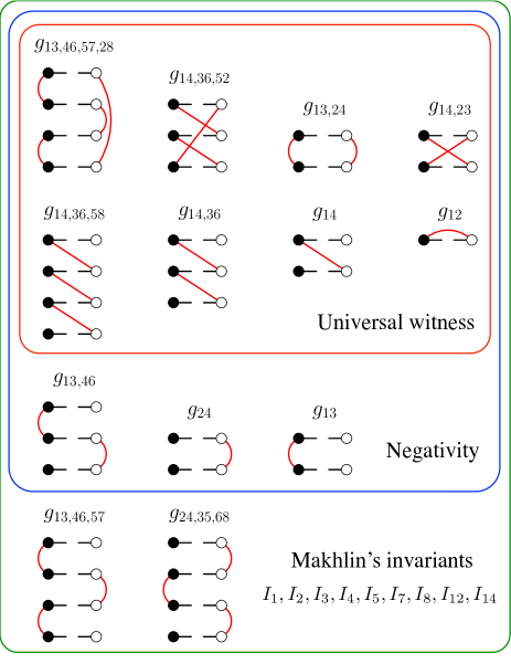
Figure 1: (color online) The minimal set of singlet-projection-based observables needed to measure 9 negativity-related Makhlin’s invariants given in Eq. (4), negativity defined in Eq. (1), and universal entanglement witness from Eq. (2). Singlet projections are marked as solid curves, dashed lines combine subsystems (black and white discs) of the same copy of $\hat{\rho}$.

We applied the techniques explained in the three presented examples to the relevant 9 invariants of Makhlin and after calculations expressed them in terms of multi-copy measurements as

$$I_{1} = -\tfrac{8}{3}\{g_{12}[g_{12}(4g_{12}-3)+6(g_{14}-2g_{14,23})]$$

$$+3g_{14,23}-6g_{14,36}+8g_{14,36,52}\},$$

$$I_{2} = 1+16g_{13,24}-4(g_{13}+g_{24}),$$

$$I_{3} = 256\left(g_{13}^{2}+4g_{13,46}+g_{24}^{2}\right),$$

$$-8(g_{13}+g_{24})+256g_{13,46,57,28}+1,$$

$$I_{4} = 1-4g_{13},$$ (10)

$$I_{5} = -4g_{24}+32g_{13,46}-64g_{13,46,57}+(1-4g_{13})^{2},$$

$$I_{7} = 1-4g_{24},$$

$$I_{8} = -4g_{13}+32g_{13,46}-64g_{24,35,68}+(1-4g_{24})^{2},$$

$$I_{12} = 1+16g_{13,46}-4(g_{13}+g_{24}),$$

$$I_{14} = 16[g_{12}^{2}(1-4g_{14})+2g_{12}(4g_{14,36}-g_{14})$$

$$-g_{14,23}+4g_{14}g_{14,23}+2g_{14,36}-8g_{14,36,58}],$$

where the relevant 13 terms $g_{12},$ $g_{13},$ $g_{14},$ $g_{24},$ $g_{13,24},$ $g_{13,46},$ $g_{14,23}$ $g_{14,36},$ $g_{14,36,52},$ $g_{13,46,57},$ $g_{24,35,68},$ $g_{13,46,57,28},$ $g_{14,36,58},$ are defined as expected values of projections on multiple singlet states as shown in Fig. 1. This result allows us to study the state-dependent parameters

$$a_{0} = -16[g_{12}^{3}+2g_{14,36,52}+$$

$$3(g_{13,24}^{2}-g_{12}^{2}g_{14}-g_{12}g_{14,23}+g_{14}g_{14,23})$$

$$-6(g_{13,46,57,28}-g_{12}g_{14,36}+g_{14,36,58})]$$

$$a_{1} = 24[g_{12}^{2}-g_{14,23}-g_{13,24}$$

$$+2(g_{13,46}-g_{12}g_{14}+g_{14,36})]$$

$$-32(g_{12}^{3}-3g_{12}g_{14,23}+2g_{14,36,52}),$$

$$a_{2} = 12(g_{13}-2g_{13,24}+g_{24}),$$

needed to calculate the negativity with Eq. (1) as functions of the multicopy observables. It turns out that these coefficients are expressed with 11 terms, i.e., $g_{12},$ $g_{13},$ $g_{14},$ $g_{24},$ $g_{13,24},$ $g_{13,46},$ $g_{14,23},$ $g_{14,36},$ $g_{14,36,52},$ $g_{13,46,57,28},$ $g_{14,36,58}.$ The universal entanglement witness in terms of singlet projections can be expressed as $\det\hat{\rho}^{\Gamma}=a_{0}/48,$ where a given two-qubit state is entangled if and only if $\det\hat{\rho}^{\Gamma}<0.$ However, to measure negativity one needs to know the values of $a_{n}$ for $n=0,1,2$. Note, that to witness entanglement it is enough to measure a smaller set of observables than for negativity. This set has 8 elements and it does not include the $g_{13},g_{24},g_{13,46}$ measurements. Thus, these measurements contain the extra information that is needed to quantify the entanglement instead of simply detecting it. Our analysis of the solutions to the quartic Eq. (1) with the help of a computer algebra system did not reveal any further reductions in the number of measurements needed to estimate the negativity.

IV Optical implementation of minimal set of multicopy projections

The singlet projection $\hat{P}$ is frequently applied to investigate the quantum properties of polarization-encoded two-qubit states Bovino05 ; Jin2012 ; Bartkiewicz13discord ; Bartkiewicz13fidelity ; Miran14 ; Bartkiewicz16fef . In this case, density matrix $\hat{\rho}$ describes a pair of polarization-encoded qubits with Pauli matrices $\hat{\sigma}_{1}=|D,D\rangle\langle D,D|-|A,A\rangle\langle A,A|,$ $\hat{\sigma}_{2}=|L,L\rangle\langle L,L|-|R,R\rangle\langle R,R|,$ and $\hat{\sigma}_{3}=|H,H\rangle\langle H,H|-|V,V\rangle\langle V,V|,$ which are expressed in terms of diagonal ($|D\rangle$), anti-diagonal ($|A\rangle$), left-circular ($|L\rangle$), right-circular ($|R\rangle$), horizontal ($|H\rangle$), and vertical ($|V\rangle$) polarization states. The singlet projection $\hat{P}$ can be implemented by measuring the anti-coalescence rate of photons that interfered on a balanced beam splitter (BS). Any two-qubit state can be expressed in a basis of the four following maximally-entangled states

$$|\Psi^{\pm}\rangle = \frac{1}{\sqrt{2}}(\mbox{$|H,V\rangle$}\pm\mbox{$|V,H\rangle$}),$$

$$|\Phi^{\pm}\rangle = \frac{1}{\sqrt{2}}(\mbox{$|H,H\rangle$}\pm\mbox{$|V,V\rangle$}).$$ (12)

We can express these two-photon states in terms of the creation operators $\hat{a}_{1e}$ and $\hat{a}_{2e}$ for polarizations $e=H,V$ (see Fig. 2), where, e.g., $\mbox{$|V,H\rangle$}=\hat{a}_{1V}^{\dagger}\hat{a}_{2H}^{\dagger}\mbox{$|0,0\rangle$}$ and $|0\rangle$ is the vacuum. Next, the states are transformed by the BS (see Fig. 2) as follows

$$U_{\rm BS}\mbox{$|\Psi^{-}\rangle$} = -\mbox{$|\Psi^{-}\rangle$},$$

$$U_{\rm BS}\mbox{$|\Psi^{+}\rangle$} = \frac{1}{\sqrt{2}}(\hat{a}_{1V}^{\dagger}\hat{a}_{1H}^{\dagger}-\hat{a}_{2V}^{\dagger}\hat{a}_{2H}^{\dagger})\mbox{$|0,0\rangle$},$$ (13)

$$U_{\rm BS}\mbox{$|\Phi^{\pm}\rangle$} = \frac{1}{2\sqrt{2}}(\hat{a}_{1H}^{\dagger 2}-\hat{a}_{2H}^{\dagger 2}\pm\hat{a}_{1V}^{\dagger 2}\mp\hat{a}_{2V}^{\dagger 2})\mbox{$|0,0\rangle$}.$$

Thus, observing anti-coalescence is equivalent to performing a singlet projection. We will use this well known fact HOM ; Pan12 to design specialized interferometers to detect and measure the entanglement of an arbitrary two-qubit state.

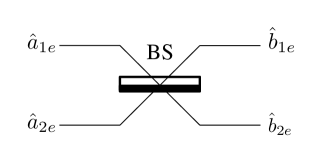
Figure 2: The 50:50 beam-splitter (BS) transforms the input annihilation operators $\hat{a}_{1e}$ and $\hat{a}_{2e}$ into output annihilation operators $\hat{b}_{1e}$ and $\hat{b}_{2e}$ according to $\hat{a}_{1e}=(\hat{b}_{1e}+\hat{b}_{2e})/\sqrt{2}$ and $\hat{a}_{2e}=(\hat{b}_{1e}-\hat{b}_{2e})/\sqrt{2},$ where $e=H,V$ represents two orthogonal polarization modes (see, e.g.,  KokBook ).

Figure 3: (color online) Interferometric configurations for measuring all independent observables from Fig. 1 with four copies of polarization-encoded $\hat{\rho}$. In configuration (b) our the interferometer can additionally measure $g_{14,36,58,72},$ which can be expressed as a function of other quantities by means of the Cayley–Hamilton theorem [see Eq. (15)]. Subsystems of a single copy are depicted as black and white discs connected with dashed lines. Photons interfere on beam splitters BS_n for $n=1,2,3,4$ and their coalescence or anti-coalescence is detected by detector modules D_n for $n=1,2,3,4$ (see, e.g., Ref. Bovino05 ). For detailed analysis of all the possible detection events see Tab. 1.

The measurements that can be used to determine the 9 relevant Makhlin’s invariants can be grouped into 6 sets. The first two sets of measurements are $S_{1}=\{g_{13,46,57,28},g_{13,46,57},g_{24,35,68},g_{13,46},g_{13},g_{24}\}$ and $S_{2}=\{g_{14,36,58},g_{14,36,58},g_{14,36},g_{14}\}.$ All the elements in these sets can be measured with interferometers that measure $g_{13,46,57,28}$ or $g_{14,36,58}$ on four copies of a given state. A proper analysis of the coincidence counts provides values of the remaining less complex measurements from this set (see Tab. 1). The next measurement set is $S_{3}=\{g_{14,36,52},g_{14,36},g_{14}\},$ where all the relevant outcomes can be obtained with an interferometer designed to measure $g_{14,36,52}$ on three copies of $\hat{\rho}$. The last three measurement sets are $S_{4}=\{g_{13,24},g_{13},g_{24}\}$, $S_{5}=\{g_{14,23},g_{14}\},$ and $S_{6}=\{g_{12}\}$ which can be measured with three interferometers operating with two or one copy of $\hat{\rho}.$ However, to measure all the above-listed quantities with four copies of $\hat{\rho}$ we need no more than four experimental configurations in total. These three configurations measure (a) $S_{1}$, (b) $S_{2},$ (c) $S_{3}$ and $S_{6}$, (d) $S_{4}$ and $S_{5}$ are shown in the respective panels of Fig. 3. Note, that some measurements (e.g., $g_{14},$ $g_{13},$ and $g_{24},$) are performed in more than one configuration (see Tab. 1).

In configuration (b) the interferometer measures observable $g_{14,36,58,72},$ which appears in the following expression for the fourth moment of $\hat{\beta},$ i.e.,

$$\mathrm{tr}\hat{\beta}^{4} = 1-16g_{14}+32(2g_{14,36}+g_{14}^{2})$$ (14)

$$+256(g_{14,36,58,72}-g_{14,36,58}).$$

Thus, we have

$$g_{14,36,58,72} = \tfrac{1}{256}[\mathrm{tr}\hat{\beta}^{4}-1+16g_{14}$$ (15)

$$-32(2g_{14,36}+g_{14}^{2})]+g_{14,36,58},$$

where $\mathrm{tr}\hat{\beta}^{4}$ is calculated using the Cayley-Hamilton theorem (see, e.g., Ref. Jing2015 ) for $\hat{\beta},$ i.e.,

$$\mathrm{tr}\hat{\beta}^{4}=\mathrm{tr}\hat{\beta}-\tfrac{1}{2}\mathrm{tr}\hat{\beta}^{2}(\mathrm{tr}^{2}\hat{\beta}-\mathrm{tr}\hat{\beta}^{2})+\mathrm{tr}\hat{\beta}\det\hat{\beta},$$ (16)

where the moments $\mathrm{tr}\hat{\beta}^{n}$ for $n=1,2,3$ are defined in Eq. (7) and the determinant $\det\hat{\beta}$ in Eq. (5) or Eq. (10). Thus, observable $g_{14,36,58,72}$ can be expressed using the observables listed in Fig. 1.

Table 1: Interpretation of detection events of the interferometers shown in Fig. 3. Each couple of detectors D_n for $n=1,2,3,4$ detects coalesce or anti-coalescence for a pair of impinging photons. The accumulated counts of (anti-) coalescence events can be grouped into $c$ coalescence or $s=a+c$ sum of coalescence ($c$) and anti-coalescence ($a$). Thus, the total number of all detection events is $Z$. Depending on the measured quantity, one can choose the required detection events in accord with Fig. 1.

D1	D2	D3	D4	Fig.  3a	Fig.  3b	Fig.  3c	Fig.  3d
s	s	s	s	$Z$	$Z$	$Z$	$Z$
s	s	s	a	$Zg_{24}$	$Zg_{14}$	$Zg_{12}$	$Zg_{14}$
s	s	a	s	$Zg_{13}$	$Zg_{14}$	$Zg_{14}$	$Zg_{14}$
s	s	a	a	$Zg_{13,46}$	$Zg_{14,36}$	$Zg_{14}g_{12}$	$Zg_{14,23}$
s	a	s	s	$Zg_{24}$	$Zg_{14}$	$Zg_{14}$	$Zg_{24}$
s	a	s	a	$Zg_{24}^{2}$	$Zg_{14}^{2}$	$Zg_{14}g_{12}$	$Zg_{24}g_{14}$
s	a	a	s	$Zg_{13,46}$	$Zg_{14,36}$	$Zg_{14,36}$	$Zg_{24}g_{14}$
s	a	a	a	$Zg_{24,35,68}$	$Zg_{14,36,58}$	$Zg_{14,36}g_{12}$	$Zg_{24}g_{14,23}$
a	s	s	s	$Zg_{13}$	$Zg_{14}$	$Zg_{14}$	$Zg_{13}$
a	s	s	a	$Zg_{13,46}$	$Zg_{14,36}$	$Zg_{14}g_{12}$	$Zg_{13}g_{14}$
a	s	a	s	$Zg_{13}^{2}$	$Zg_{14}^{2}$	$Zg_{14,36}$	$Zg_{13}g_{14}$
a	s	a	a	$Zg_{13,46,57}$	$Zg_{14,36,58}$	$Zg_{14,36}g_{12}$	$Zg_{13}g_{14,23}$
a	a	s	s	$Zg_{13,46}$	$Zg_{14,36}$	$Zg_{14,36}$	$Zg_{13,24}$
a	a	s	a	$Zg_{24,35,68}$	$Zg_{14,36,58}$	$Zg_{14,36}g_{12}$	$Zg_{13,24}$
a	a	a	s	$Zg_{13,46,57}$	$Zg_{14,36,58}$	$Zg_{14,36,52}$	$Zg_{13,24}g_{14}$
a	a	a	a	$Zg_{13,46,57,28}$	$Zg_{14,36,58,72}$	$Zg_{14,36,52}g_{12}$	$Zg_{13,24}g_{14,23}$

V Conclusions

Finding a minimal set of 13 interferometric quantities for expressing the relevant 9 Makhlin’s invariants (11 for negativity, and 8 for detecting entanglement of a given two-qubit state) is the main results of this paper. It explicitly proves that one has to perform more measurements to reconstruct the state (i.e., 15 measurements) than, e.g., to measure the negativity (i.e., 11 measurements). In contrast to the previous works Carteret05 ; Bart15a ; Bart15b , here we explicitly demonstrated that all the necessary data for detecting or quantifying the entanglement can be directly measured without collecting irrelevant information about the state. This was not apparent before, because the previously proposed measurement schemes were designed for measuring moments of a given partially transposed density matrix Carteret05 ; Bart15a ; Bart15b and required ignoring some detection events or output modes, or using ancillary entangled states. The interferometers shown in Fig. 2 measure only the functions of 13 observables depicted in Fig. 1 and they cannot be further simplified without loosing the ability to measure the entanglement or the relevant 9 Makhlin’s invariants. Measuring local invariants with linear optics requires collecting less data than performing a complete quantum state tomography, which for a two-qubit state requires 15 measurements. Hence, we also demonstrated that local invariants are both useful theoretical concept for designing specialized quantum interferometers and that their direct measurement within the framework of linear optics does not require performing complete quantum state tomography.

The described set of 11 observables is the minimal set of measurements needed to determine the value of the negativity. Because one cannot express the basic measurements as functions of each other, the presented set seems impossible to reduce further. Moreover, any attempt to discard some of the measurements will change the values of parameters $a_{n}$ for $n=0,1,..2$ in the characteristic equation, thus, the value of $N$ calculated from Eq. (1). In contrast to the results presented in Ref. Bart15a ; Carteret05 , we do not need ancillary qubits and we use information from all output modes.

Our results provide a new perspective on the phenomenon of quantum entanglement in terms of entanglement cost under PPT operations. We demonstrated in Figs. 1 and 2 that two-qubit entanglement can be fully described using two-photon interference events between subsystems of at most four copies of a given state. As explicitly shown in Tab. 1, our approach gives us only the information needed to measure negativity, universal entanglement witness, and the relevant Makhlin’s invariants. All the measured information can be interpreted in terms of the minimal set of observables depicted in Fig. 1. This approach only requires using beam splitters and photon detectors, i.e., the basic building blocks of quantum information processing within the framework of linear optics KokBook . However, singlet projections on multilevel systems can be also implemented in, e.g., solid state systems  Tanaka14 .

The presented general approach can be also used for measuring a different type of quantum correlations than quantum entanglement  Modi12 , i.e. quantum discord. This type of quantum correlations is hard to compute (NP-complete) as shown in Ref. Huang14 . Note, that measuring or detecting geometric quantum discord could require more complex measurements than in the case of entanglement, as described in Refs. Jin2012 ; Bartkiewicz13discord .

One of the open problems related to the topic of this paper is the degree of complexity of analogous interferometers used for entanglement measures other than negativity. By studying this problem one could categorize the entanglement measures operationally with respect to the amount of experimental effort required to measure them. We expect that this would also give us some intuition about the experimental differences between the particular entanglement measures like, e.g., concurrence and negativity, whose definitions are often too abstract to directly compare.

- (1) M. Grassl, M Rötteler, and Thomas Beth, “Computing local invariants of quantum-bit systems ,” Phys. Rev. A 58 1833 (1999).
- (2) E. M. Rains, “Polynomial invariants of quantum codes,” IEEE Trans. Inf. Theory 46, 54 (2000).
- (3) Y. Makhlin, “Nonlocal properties of two-qubit gates and mixed states and optimization of quantum computations,” Quantum Inf. Process. 1 (4), 243 (2002).
- (4) L. Koponen, V. Bergholm, M. M. Salomaa, “A discrete quantum invariant for quantum gates,” Quant. Inf. Comput. 6, 058 (2005).
- (5) H. de Riedmatten, I. Marcikic, W. Tittel, H. Zbinden, D. Collins, and N. Gisin, “Long Distance Quantum Teleportation in a Quantum Relay Configuration,” Phys. Rev. Lett. 92, 047904 (2004).
- (6) A. K. Ekert, “Quantum cryptography based on Bell’s theorem,” Phys. Rev. Lett. 67, 661 (1991).
- (7) R. King and T. Welsh, “Qubits and invariant theory,” J. Phys.: Conf. Ser. 30, 1 (2006).
- (8) N. Jing, S.-M. Fei, M. Li, X. Li-Jost, and T. Zhang, “Local unitary invariants of generic multiqubit states”, Phys. Rev. A 92, 022306 (2015).
- (9) E. Schrödinger, “Discussion of Probability Relations between Separated Systems,” Proc. Camb. Phil. Soc. 31, 555 (1935).
- (10) A. Einstein, N. Podolsky, and B. Rosen, “Can Quantum-Mechanical Description of Physical Reality Be Considered Complete?,” Phys. Rev. 47, 777 (1935).
- (11) A. Osterloh and J. Siewert, “Invariant-based entanglement monotones as expectation values and their experimental detection,” Phys. Rev. A 86 042302 (2012).
- (12) H. A. Carteret, “Noiseless Quantum Circuits for the Peres Separability Criterion,” Phys. Rev. Lett. 94, 040502 (2005).
- (13) J. Kempe, “Multiparticle entanglement and its applications to cryptography,” Phys. Rev. A 60, 910 (1999).
- (14) A. Peres, “Separability Criterion for Density Matrices,” Phys. Rev. Lett. 77, 1413 (1996).
- (15) M. Horodecki, P. Horodecki, and R. Horodecki, “Separability of mixed states: necessary and sufficient conditions,” Phys. Lett. A 223, 1 (1996).
- (16) K. Bartkiewicz, P. Horodecki, K. Lemr, A. Miranowicz, and K. Życzkowski, “Method for universal detection of two-photon polarization entanglement,” Phys. Rev. A 91, 032315 (2015).
- (17) K. Bartkiewicz, J. Beran, K. Lemr, M. Norek, and A. Miranowicz, “Quantifying entanglement of a two-qubit system via measurable and invariant moments of its partially transposed density matrix”, Phys. Rev. A 91, 022323 (2015).
- (18) K. Życzkowski, P. Horodecki, A. Sanpera, and M. Lewenstein, “Volume of the set of separable states,” Phys. Rev. A 58, 883 (1998).
- (19) G. Vidal and R. F. Werner, “Computable measure of entanglement,” Phys. Rev. A 65, 032314 (2002).
- (20) W. K. Wootters, “Entanglement of Formation of an Arbitrary State of Two Qubits,” Phys. Rev. Lett. 80, 2245 (1998).
- (21) G. Chaudhary and V. Ravishankar, “Optimal observables to determine entanglement of a two qubit state,” Eur. Phys. J. D 70, 10 (2016).
- (22) H. A. Carteret, “Exact interferometers for the concurrence and residual 3-tangle,” e-print quant-ph/0309212v7.
- (23) S. P. Walborn, P. H. Souto Ribeiro, L. Davidovich, F. Mintert, and A. Buchleitner, “Experimental determination of entanglement with a single measurement,” Nature (London) 440, 1022 (2006).
- (24) L. Aolita and F. Mintert, “Measuring Multipartite Concurrence with a Single Factorizable Observable,” Phys. Rev. Lett. 97, 050501 (2006).
- (25) L. Zhou, Y.-B. Sheng, “Detection of nonlocal atomic entanglement assisted by single photons,” Phys. Rev. A 90, 024301 (2014).
- (26) F. Verstraete, K. Audenaert, J. Dehaene and B. De Moor, “A comparison of the entanglement measures negativity and concurrence,” J. Phys. A 34, 10327 (2001).
- (27) A. Miranowicz and A. Grudka, “Ordering two-qubit states with concurrence and negativity,” Phys. Rev. A 70, 032326 (2004).
- (28) I. Bengtsson and K. Życzkowski, Geometry of Quantum States (Cambridge University Press, Cambridge, 2006).
- (29) R. Horodecki, P. Horodecki, M. Horodecki, and K. Horodecki, “Quantum entanglement,” Rev. Mod. Phys. 81, 865 (2009).
- (30) W. P. Schleich and H. Walther, Elements of Quantum Information (Wiley-VCH, Weinheim, 2007).
- (31) O. Krueger and R.F. Werner (eds.), Some Open Problems in Quantum Information Theory, e-print quant-ph/0504166.
- (32) O. Gühne, M. Reimpell, and R.F. Werner, “Estimating entanglement measures in experiments,” Phys. Rev. Lett. 98, 110502 (2007).
- (33) F. Mintert, “Entanglement measures as physical observables,” Appl. Phys. B 89, 493 (2007).
- (34) O. Gühne and G. Tóth, “Entanglement detection,” Phys. Rep. 474, 1 (2009).
- (35) L. Gurvits, “Classical complexity and quantum entanglement,” J. Comput. Syst. Sci. 69, 448 (2004).
- (36) S. Gharibian, “Strong NP-Hardness of the Quantum Separability Problem,” Quantum Inf. and Comput., 10, 343 (2010).
- (37) D. Lu, T. Xin, N. Yu, Z. Ji, J. Chen, G. Long, J. Baugh, X. Peng, B. Zeng, and R. Laflamme, “Tomography is Necessary for Universal Entanglement Detection with Single-Copy Observables,” Phys. Rev. Lett. 116, 230501 (2016).
- (38) P. Horodecki and A. Ekert, “Method for Direct Detection of Quantum Entanglement,” Phys. Rev. Lett. 89, 127902 (2002).
- (39) P. Horodecki, “From limits of quantum operations to multicopy entanglement witnesses and state-spectrum estimation,” Phys. Rev. A 68, 052101 (2003).
- (40) R. Augusiak, M. Demianowicz, and P. Horodecki, “Universal observable detecting all two-qubit entanglement and determinant-based separability tests,” Phys. Rev. A 77, 030301 (2008).
- (41) T. O. Maciel and R. O. Vianna, “Viable entanglement detection of unknown mixed states in low dimensions,” Phys. Rev. A 90, 032325 (2009).
- (42) M. Demianowicz, “Reexamination of determinant-based separability test for two qubits,” Phys. Rev. A 83, 034301 (2011).
- (43) H. S. Park, S. S. B. Lee, H. Kim, S. K. Choi, and H. S. Sim, “Construction of an Optimal Witness for Unknown Two-Qubit Entanglement,” Phys. Rev. Lett. 105, 230404 (2010).
- (44) K. Bartkiewicz, K. Lemr, A. Černoch, A. Miranowicz, “Bell nonlocality and fully-entangled fraction measured in an entanglement-swapping device without quantum state tomography,” e-print quant-ph/1609.09653v1.
- (45) Ł. Rudnicki, P. Horodecki, and K. Życzkowski, “Collective Uncertainty Entanglement Test,” Phys. Rev. Lett. 107, 150502 (2011).
- (46) K. Lemr, K. Bartkiewicz, and A. Černoch, “Experimental measurement of collective nonlinear entanglement witness for two qubits,” Phys. Rev. A 94, 052334 (2016).
- (47) F. A. Bovino, G. Castagnoli, A. Ekert, P. Horodecki, C. Moura Alves, and A. V. Sergienko, “Direct Measurement of Nonlinear Properties of Bipartite Quantum States,” Phys. Rev. Lett. 95, 240407 (2005).
- (48) K. Audenaert, M. B. Plenio, and J. Eisert, “Entanglement Cost under Positive-Partial-Transpose-Preserving Operations,” Phys. Rev. Lett. 90, 027901 (2003).
- (49) S. Ishizaka, “Binegativity and geometry of entangled states in two qubits,” Phys. Rev. A 69, 020301(R) (2004).
- (50) C. Eltschka and J. Siewert, “Negativity as an Estimator of Entanglement Dimension,” Phys. Rev. Lett. 111, 100503 (2013).
- (51) S. Rana, “Negative eigenvalues of partial transposition of arbitrary bipartite states,” Phys. Rev. A 87, 054301 (2013); A. Sanpera, R. Tarrach, and G. Vidal, “Local description of quantum inseparability,” ibid. 58, 826 (1998).
- (52) A. Miranowicz, K. Bartkiewicz, A. Pathak, J. Peřina, Jr., Y.-N. Chen, and F. Nori, “Statistical mixtures of states can be more quantum than their superpositions: Comparison of nonclassicality measures for single-qubit states,” Phys. Rev. A 91, 042309 (2015).
- (53) J. Jin, F. Zhang, C. Yu and H. Song, “Direct scheme for measuring the geometric quantum discord,” J. Phys. A 45, 115308 (2012).
- (54) K. Bartkiewicz, K. Lemr, A. Černoch, and J. Soubusta, “Measuring nonclassical correlations of two-photon states,” Phys. Rev. A 87, 062102 (2013).
- (55) K. Bartkiewicz, K. Lemr, and A. Miranowicz, “Direct method for measuring of purity, superfidelity, and subfidelity of photonic two-qubit mixed states,” Phys. Rev. A 88, 052104 (2013).
- (56) A. Miranowicz, K. Bartkiewicz, J. Perina Jr., M. Koashi, N. Imoto, and F. Nori, “Optimal two-qubit tomography based on local and global measurements”, Phys. Rev. A 90, 062123 (2014).
- (57) C. K. Hong, Z. Y. Ou, L. Mandel, “Measurement of subpicosecond time intervals between two photons by interference,” Phys. Rev. Lett. 59, 2044 (1987).
- (58) J.-W. Pan, Z.-B. Chen, C.-Y. Lu, H. Weinfurter, A. Zeilinger, and M. Żukowski “Multiphoton entanglement and interferometry,” Rev. Mod. Phys. 84, 777 (2012).
- (59) P. Kok and B. W. Lovett, Introduction to Optical Quantum Information Processing (Cambridge University Press, Cambridge, 2010).
- (60) T. Tanaka, Y. Ota, M. Kanazawa, G. Kimura, H. Nakazato, and F. Nori, “Determining eigenvalues of a density matrix with minimal information in a single experimental setting”, Phys. Rev. A 89, 012117 (2014).
- (61) K. Modi, A. Brodutch, H. Cable, T. Paterek, V. Vedral, “The classical-quantum boundary for correlations: discord and related measures,” Rev. Mod. Phys. 84, 1655-1707 (2012).
- (62) Y. Huang, “Computing quantum discord is NP-complete,” New J. Phys. 16, 033027 (2014).