Gauging spatial symmetries and the classification of topological crystalline phases
Abstract
We put the theory of interacting topological crystalline phases on a systematic footing. These are topological phases protected by space-group symmetries. Our central tool is an elucidation of what it means to “gauge” such symmetries. We introduce the notion of a crystalline topological liquid, and argue that most (and perhaps all) phases of interest are likely to satisfy this criterion. We prove a Crystalline Equivalence Principle, which states that in Euclidean space, crystalline topological liquids with symmetry group are in one-to-one correspondence with topological phases protected by the same symmetry , but acting internally, where if an element of is orientation-reversing, it is realized as an anti-unitary symmetry in the internal symmetry group. As an example, we explicitly compute, using group cohomology, a partial classification of bosonic symmetry-protected topological (SPT) phases protected by crystalline symmetries in (3+1)-D for 227 of the 230 space groups. For the 65 space groups not containing orientation-reversing elements (Sohncke groups), there are no cobordism invariants which may contribute phases beyond group cohomology, and so we conjecture our classification is complete.
Symmetry is an important feature of many physical systems. Many phases of matter can be characterized in part by the way the symmetry is implemented. For example, liquids and solids are distinguished by whether or not they spontaneously break spatial symmetries. In fact, it was once thought that all known phases could be distinguished by their symmetries and that all continuous phase transitions were spontaneous symmetry breaking transitions. The discovery of topological orderWen (1990) showed that, at zero temperature, there are quantum phases of matter that can be distinguished by patterns of long-range entanglement without the need to invoke symmetry. However, even for topological phases symmetry is important. Any symmetry that is not spontaneously broken in a topological phase must have some action on the topological structure of the phase, and different such patterns can distinguish different phases. Even a phase of matter that is trivial without symmetry can become non-trivial when considering how symmetry is implemented. Topological phases distinguished by symmetry are known as symmetry-enriched topological (SET)Maciejko et al. (2010); Essin and Hermele (2013); Lu and Vishwanath (2013); Mesaros and Ran (2013); Hung and Wen (2013); Barkeshli et al. (2014); Cheng et al. (2015a) or symmetry-protected topological (SPT)Gu and Wen (2009); Pollmann et al. (2010, 2012); Fidkowski and Kitaev (2010); Chen et al. (2010, 2011a); Schuch et al. (2011); Fidkowski and Kitaev (2011); Chen et al. (2013, 2011b); Vishwanath and Senthil (2013); Wang et al. (2014); Kapustin (2014); Gu and Wen (2014); Else and Nayak (2014); Burnell et al. (2014); Wang et al. (2015); Cheng et al. (2015b) depending on whether they are nontrivial or trivial without symmetry, respectively.
For internal symmetries, which do not move points in space around, very general and powerful ways of understanding SPT and SET phases have been formulated in terms of mathematical notions such as group cohomologyChen et al. (2013), category theoryBarkeshli et al. (2014), and cobordismsKapustin (2014); Kapustin et al. (2015). On the other hand, such techniques have not, so far, been extended to the case of space group symmetries. We refer to these topological phases enriched by space-group symmetries as topological crystalline phases. This is a significant omission because any system which arranges itself into a regular crystal lattice is invariant under one of 230 space groups in three dimensions. Fermionic phases of matter protected by space-group symmetries are called topological crystalline insulators or topological crystalline superconductors depending on whether charge is conserved Fu (2011); Hsieh et al. (2012); Dziawa et al. (2012); Tanaka et al. (2012); Xu et al. (2012); Zhang et al. (2013). Progress towards a general classification in free-fermion systems has been made Fang et al. (2012, 2013); Chiu et al. (2013); Morimoto and Furusaki (2013); Slager et al. (2013); Shiozaki and Sato (2014); Chiu et al. (2016) and some understanding of the effect of interactions been achieved Isobe and Fu (2015); Hsieh et al. (2014a); Qi and Fu (2015); Yoshida and Furusaki (2015); Song and Schnyder (2016). Meanwhile, intrinsically strongly interacting phases protected by spatial symmetries have also been found Wen (2002); Essin and Hermele (2013); Hsieh et al. (2014b); Cho et al. (2015); Yoshida et al. (2015); Barkeshli et al. (2014); Lapa et al. (2016); You and Xu (2014); Hermele and Chen (2016); Cheng et al. (2015c); Jiang and Ran (2016). In particular Ref. Song et al. (2016) gave an approach for deriving the general classification of interacting SPT phases protected by a group of spatial symmetries that leave a given point invariant. However, for SETs and/or general space groups, there is so far no systematic theory analogous to the one that exists for internal symmetries, except in one dimension Chen et al. (2011c). Our goal in this paper is to fill this gap.
We will adopt two complementary and related viewpoints to the classification. The first viewpoint is in terms of topological quantum field theories (TQFTs), which are believed to describe the low-energy physics of topological phases. We state and motivate a proposal for how to implement a spatial symmetry in a TQFT.
Our second, more concrete, viewpoint is based on the idea of understanding the SPT or SET order of a system by studying its response to a gauge field. For example, SPTs in (2+1)-D protected by an internal symmetry can be identified by the topological response to a gauge field. All such possible responses are described by the Chern-Simons action
| (1) |
The coefficient has a physical interpretation as the quantized Hall conductance. Because it is quantized, the only way to get between systems with different values of is if symmetry is broken or the gap closes. Further, since this is the only term that may appear, we learn that the different SPTs in 2+1D are labelled by this integer. We call this procedure of coupling a -symmetric system to a background gauge field “gauging” the symmetry, though strictly speaking we do not consider making the gauge field dynamical. Stricter terminology would call the dynamical gauge theory the result of gauging and our procedure the first step, called equivariantization, a mouthful, or pregauging. Many of the general approaches to SPT and SET phases can be formulated in terms of gaugingDijkgraaf and Witten (1990); Levin and Gu (2012); Hung and Wen (2013); Barkeshli et al. (2014).
We want to apply similar approaches to the study of systems with spatial symmetry. So we will ask the question
Question 1.
What does it mean to gauge a spatial symmetry?
We will give what we believe to be the definitive answer to this question, motivated by the intuition of “gauge fluxes” which for spatial symmetries are crystallographic defects such as dislocations and disclinations. There seems to be a natural generalization of this to symmetries which act on spacetime as well, such as time reversal symmetry or time translation. We will mention briefly this generalization and how the classification extends to these spacetime symmetries, where it agrees with known group cohomology classifications of time reversal-invariant and Floquet SPTs, respectively.
Using the two viewpoints mentioned above, we will elucidate the general theory of crystalline topological phases. Our results are based on a key physical assumption, namely that the phases of matter under consideration are crystalline topological liquid, which roughly means that, although crystalline, they preserve a certain degree of “fluidity” in the low-energy limit. The idea is motivated by the notion of “topological liquids” which have an IR limit that is described by a topological quantum field theory (TQFT), i.e. the long-range physics is only sensitive to the topology of the background manifold. This is in contrast to “fracton” topological phasesHaah (2011); Yoshida (2013); Vijay et al. (2016); Williamson (2016) where no such topological IR limit exists111Although see Section VII.. Crystalline topological liquids are a generalization of topological liquids to systems with crystal symmetries.
The main result of this paper is the following.
Crystalline Equivalence Principle: The classification of crystalline topological liquids with spatial symmetry group is the same as the classification of topological phases with internal symmetry .
Compare Ref. Else and Nayak, 2016, where a similar principle was conjectured for symmetry groups containing time translation symmetry. This result holds for systems living on a contractible space, ie. Euclidean space in dimensions. On other manifolds, for example Euclidean space with some holes, some new things happen. We note for this correspondence, orientation-reversing symmetries in the space group must correspond to anti-unitary symmetries in the internal group.
| Number | Name | Classification |
|---|---|---|
| 1 | 0 | |
| 2 | ||
| 3 | ||
| 4 | 0 | |
| 5 | ||
| 6 | ||
| 7 | ||
| 8 | ||
| 9 | ||
| 10 | ||
| 11 | ||
| 12 | ||
| 13 | ||
| 14 | ||
| 15 | ||
| 16 | ||
| 17 |
We emphasize that the Crystalline Equivalence Principle is expected to hold for both bosonic and fermionic222There are some caveats for fermionic systems: systems with , where is a reflection, are in correspondence with systems with , where is time-reversal, and vice versa. systems, and for both SPT and SET phases. As an example of results that one can deduce from this general principle, we find that bosonic SPT phases protected by orientation-preserving unitary spatial symmetry are classified by the group cohomology , since that is the classification of internal SPTs with symmetry (See Appendix A for more details on the definition of .) This agrees with a recent classification of a class of tensor networks with spatial symmetriesJiang and Ran (2016). In (3+1)-D, for space groups containing orientation-reversing transformations, this classification is expected to be incomplete, just as it is for internal symmetry groups containing anti-unitary symmetriesKapustin (2014). Applying the principle to fermionic systems, one obtains a partial classification of fermionic SPT’s protected by space-group symmetries from “group supercohomology” Gu and Wen (2014) and a complete classification of fermionic crystalline SPT’s from cobordism theory Kapustin et al. (2015), with some caveats. We attempt this in section VII.2 for crystalline topological superconductors and insulators.
Our results allow for the classification to be explicitly computed in many cases. For example, Table 1 shows the classification of bosonic SPT phases protected by space-group symmetry in (2+1)-D as obtained from group cohomology. For more details of how Table 1 was computed, and the (3+1)-D version of the table, see Appendix B.
The outline of our paper is as follows. In Section I, we introduce the notion of a crystalline topological liquid. Then, in Section II we introduce the key ideas involved in gauging a spatial symmetry. Specifically, in section II.1 we discuss our definition of crystalline gauge field. Then in II.2 we argue that crystalline topological liquids naturally couple to such crystalline gauge fields. In II.3 we use the gauging picture to derive the Crystalline Equivalence Principle, which applies to the physically relevant case of phases of matter in contractible space . In II.4 we discuss extensions to non-contractible spaces and a general classification result for crystalline gauge fields.
In Section III we give a construction of many crystalline topological liquids from ordinary topological liquids by considering systems which carry both a spatial symmetry and an internal symmetry.
In Section IV we describe our approach towards classifying crystalline topological liquids using topological response. In IV.1, this is defined in terms of fusion and braiding of symmetry fluxes. In IV.2 it is described in terms of effective topological actions. Finally, in IV.3, we give many examples of crystalline gauge backgrounds and compute the resulting partition functions in exactly solvable models. This section is particularly important, as it elucidates where some of the familiar features of ordinary SPT phases appear in crystalline SPT phases.
In Section V, we describe how our methods can be placed into a general context of position-dependent topological limit, and discuss implications of emergent Lorentz invariance or lack thereof.
In Section VI, we derive several general structural results about the classification of crystalline SPTs (invertible crystalline topological liquids).
We give generalizations of our methods in Section VII, including Floquet phases in VII.1 and phases beyond ordinary equivariant cohomology in VII.2 including fermions. In VII.3 we discuss how our methods apply to topological terms of sigma models.
In Section VIII, we describe some ways in which our crystalline topological liquid assumption can fail and include some comments about fracton phases.
In Section IX we discuss questions for future work.
We hope this paper will inspire the discovery of many curious quantum crystals.
I The topological limit of a crystalline topological phase
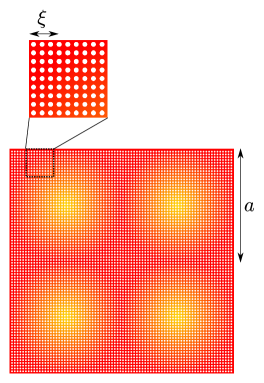
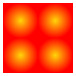
In this section, we will briefly outline the arguments based on topological quantum field theory (TQFT) which lead to the Crystalline Equivalence Principle. The mathematical details are left to Section V. The underlying physical concept is that of a smooth state. A smooth state is a ground state of a lattice Hamiltonian that is defined on a lattice which is much finer than the unit cell with respect to the translation symmetry, such that the lattice spacing and the correlation length are much smaller than the minimum radius of spatial variation within the unit cell. The condition (where is the unit cell size) was discussed as an assumption for classifying crystalline phases in Ref. Hua (2017); our “smooth state” assumption is slightly stronger since we require . This implies the condition of Ref. Hua (2017) since , but the converse need not be true if there are regions in the unit cell where spatial variation happens rapidly (so that ).
A smooth state might not seem like the kind of system one would normally consider; a physical example would be a graphene heterostructure in which a lattice mismatch between two layers results in a Moire pattern with very large unit cell Hunt et al. (2013). Nevertheless, it is reasonable to expect that the classification of smooth states would be the same as the classification of states in general. We will leave a rigorous proof for future work; presently, we merely state it as a conjecture and examine the consequences.
A very important property of a smooth state is that it can be coarse-grained while preserving the spatial symmetries. This is allowed only so long as the coarse-grained lattice is still small compared to the unit cell size, but given the assumption this still allows us to reach a “topological limit”, by which we mean that becomes much smaller than the coarse-grained lattice spacing. Importantly, since the RG can take place in the neighborhood of any given point in the unit cell, the effective field theory that we obtain in this topological limit will still be spatially-dependent. (For this reason, we will avoid referring to the topological limit as an “IR limit”, which would be misleading since the unit cell size – but not the lattice spacing! – is still an important length scale).
We expect that this topological limit will, as in the case of systems without spatial symmetries, be described by a topological quantum field theory (TQFT). In fact, given the afore-mentioned spatial dependence, it should be described by a spatially-dependent TQFT. We give the precise mathematical definition of this concept in Section V.
Hence, we can define
Definition 1.
A crystalline topological liquid is a phase of matter that is characterized by a spatially-dependent TQFT acted upon by spatial symmetries.
We expect that this class of systems is quite large. Certainly, it includes ordinary topological liquids (which, by definition, have no explicit spatial symmetries and can be characterized by a spatially-constant TQFT). Moreover, spatially-dependent TQFTs can capture a wide range of other topological crystalline phenomena, as we shall see.
In Section V, we sketch a proof that on contractible spaces, spatially-dependent TQFTs with spatial symmetries are in one to one correspondence with spatially constant TQFTs with internal symmetries. Since the latter are expected to characterize topological phases with internal symmetries, the Crystalline Equivalence Principle follows. In the following sections, we we will discuss how to understand this result in more concrete ways without resorting to the highly abstract formalism of TQFTs.
II Crystalline gauge Fields
II.1 Gauge fluxes and crystal defects
In order to understand crystalline topological phases, we want to study what it might mean to couple to a background gauge field for a symmetry group involving some transformation of space itself. More generally, we believe a framework exists where one can also consider symmetries that transform space-time. However, for simplicity and to maintain contact with Hamiltonian models we will focus on purely spatial symmetries. We call our object of study the crystalline gauge field.
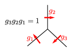
A special case of a background gauge field is an isolated gauge flux. Isolated gauge fluxes are familiar objects for internal symmetries. They are objects in space of codimension 2 (i.e. points in 2-D, curves in 3-D) which are labelled by a group element , and a particle moving all the way around one is acted upon by . Actually, for a non-Abelian group only the conjugacy class of is gauge-invariant.
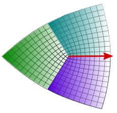
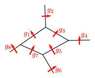
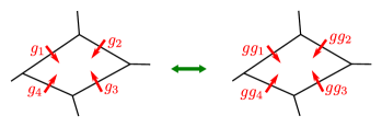
Gauge fluxes for spatial symmetries are also labelled by conjugacy classes of . They are also well-known, but not under that name; they are more commonly referred to as crystal defects. For example, a gauge flux for translational symmetry is a dislocation and a gauge flux for a rotational symmetry is a disclination (Fig 2). In 3d, the direction of dislocation does not have to be in the plane perpendicular to the defect, as in a screw dislocation. A defect for reflection symmetry is like the Möbius band (a cross cap). For a glide reflection we also insert a shift in the lattice as we go around the band. We will see how this zoo of defect configurations is tamed by topology.


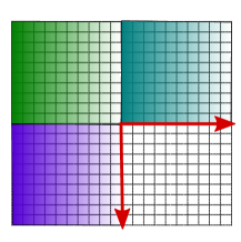
Generalizing these examples, we can give a systematic definition of crystalline gauge flux, and more generally of a crystalline gauge field. For motivation, one can look again at Fig 2. The original lattice is a regular square or kagome lattice. The crucial property the defect lattice is that away from the singular point in the middle, it looks locally the same as , meaning that in a neighborhood of every face except the central one there is an invertible map sending to . However, there is no global map sending to . Indeed, if we try to extend the domain of our map, we will eventually create a discontinuity after encircling the singularity. This is shown in Fig 3. For the 90 degree angular defect, the discontinuity is a branch cut such that the limits on either side are related by a 90 degree rotation. For a crystal defect, this discontinuity is always by a transformation and labels the symmetry flux of the defect.
To further motivate the definition, let us recall the definition of a gauge field for an internal (discrete) symmetry. Gauge fields for discrete symmetries are somewhat more esoteric than gauge fields for continuous groups (like the familiar electromagnetic vector potential ). One way to think about them is that they encode “twisted boundary conditions”. For example, threading a non-trivial gauge flux for an Ising symmetry through a system living on a circle means that we make a cut and identify spin-up on one side of the cut with spin-down on the other side of the cut (“anti-periodic boundary conditions”). In general, to specify a gauge field on a manifold we can build up out of “patches”. The boundaries between patches (“domain walls”) are “twisted” by an element of the symmetry group (“transition functions”), which tells us how to identify the patches. A discrete gauge field must be “flat”, which is to say there can be no non-trivial holonomy around a vertex where several patches intersect, as shown in Figure 4. This is to say there is no -flux through the vertices (or along such line-like junctions in a 3d picture). There is some inherent gauge freedom: firstly, we can merge or split patches, provided that the boundaries thus created or destroyed are twisted by the trivial element ; secondly, we can apply an element of the symmetry group to a given patch , which has the effect of multiplying the twist carried by the boundaries of this patch by . This gauge freedom relates two different representations of the same gauge field. More abstractly (but equivalently), we can define a gauge field as a principal -bundle over Nakahara (2003).
As an example, we can consider a -flux at the origin of the plane. This -flux is defined as a gauge field on the plane minus the origin. It may be defined using a single (simply-connected) patch which meets itself along a domain wall extending from the origin to infinity. This domain wall is labeled with the transition function , indicating that a point charge taking along a path encircling the origin will return to its original position with any internal degrees of freedom transformed by the symmetry . The similarity between the internal symmetry flux and the crystal defect is striking. It leads us to identify the role of the branch cut in the latter with the domain wall of the former.
With this identification in hand, we are ready to state our definition of crystalline gauge field, by directly generalizing the patches picture of internal symmetry gauge fields. An important novelty will be that the lattice geometry is defined by the crystalline gauge background. That is, we fix our physical space containing the lattice . is usually , a torus, or some related spacetime. acts on preserving . The lattice with defects will be embedded in a different space . For example, in the disclination, is the plane minus the origin.
To specify a crystalline gauge field, we will start with the same data we had before: a collection of patches dividing , with domain walls between intersecting patches labelled by elements , with the flatness condition imposed over all contractible loops. This is the definition of an internal symmetry gauge field, but it is not the end of the story, because as we saw in the examples above, there is an extra feature of crystalline gauge fluxes which needs to be captured: a map . This represents the (continuum limit) of the identification between the lattices embedded in and embedded in . Inside each patch , this map is continuous, but on the boundaries between intersecting patches we impose the twisted continuity condition that for any , the limit of as in and the limit of as in are related in from the former to the latter by application of . For example, in Figure 3, the different colored quadrants are patches on (which in this case is the punctured plane , and the thick red line denotes a boundary between patches which is twisted by a degree clockwise rotation as we pass from the teal patch to the violet patch. We impose the same gauge freedom as before [Figure 4(c) and 4(d)], except that when we act on a patch by , as shown in Figure 4(d), then inside the patch we replace the function according to .
There is a final condition we need to impose, related to the orientation (or lack thereof) of the manifold . It is standard lore that a topological phase that is not reflection invariant cannot be put on an unorientable manifold, and moreover, that for a reflection invariant system, putting it on a unorientable manifold is essentially threading a “flux” of the reflection symmetry. So in order to enforce compatibility with these notions, we define if acts in an orientation-reversing way on , and otherwise. For any closed loop in , we can define the “flux” , which is the product of the twist over each boundary crossed by . We also define depending on whether going around the loop would reverse the orientation on . We require that .
For completeness, we will also formulate a more abstract mathematical definition. Basically we are specifying some extra data on top of a principal -bundle. Formally, we have
Definition 2.
A crystalline gauge field is a pair , where is a principal bundle, and is a continuous map satisfying satisfying for all , . We require that the homomorphism (where if has orientation-reversing action on ) reduces to the orientation bundle of . We say that two pairs , represent the same crystalline gauge field if the principal -bundles and are isomorphic by a map such that .
The map in the definition above always induces a map from into . Hence, we have the following commutative diagram:
| (2) |
It should be clear, from the disclination example, that crystalline gauge fields can describe the crystal defects which were our original motivation. However, now that have given a general definition, we had better ask whether all crystalline gauge fields admit such a physical interpretation. In particular, there ought to be a well-defined sense of what it means to couple to a general crystalline gauge field.
For internal symmetries it is familiar how to couple to a gauge field, at least when that gauge field lives on . Given a gauge field for a (discrete) internal symmetry , described using patches and transition functions, and given a Hamiltonian that commutes with the symmetry, we can define a Hamiltonian that describes the system coupled to the gauge field. To do this, we assume that can be written as a sum of local terms. Then, contains a local term for each local term in . The terms in which act only within a patch carry over to without change, while for terms in which act in multiple patches, we must first perform a gauge transformation so that the term acts in a single patch, add it to the Hamiltonian, and then reverse that gauge transformation. See, for example Barkeshli et al. (2014).
Now suppose that we want to do the same thing for crystalline gauge fields. For crystal defects (for example, the disclination in Figure 3) it should be clear how to do this; locally, the defect lattice looks the same as the original lattice, so we just pull local terms in back into . On the other hand, this construction doesn’t necessarily work for a general crystalline gauge field. We have to impose a condition which we call rigidity.
Definition 3.
A crystalline gauge field (expressed in terms of patches, twisted boundary conditions, and a map ) is rigid if near any point that maps into a lattice point in under , there exists a local neighborhood containing such that, after making a gauge transformation such that is contained in a single patch, is injective (one-to-one) when restricted to ; and, moreover, the image of under contains all lattice points that are coupled to by a term in the Hamiltonian.333For certain applications, this last condition may be relaxed near a boundary of . Terms in the Hamiltonian which fall of the edge may need to be discarded or modified in some arbitrary manner.
This somewhat technical definition is best understood by considering examples of crystalline gauge fields which are not rigid. An extreme example is the case where is the constant function: there is some such that for all . In other words, every point in gets identified with a single point in . If the Hamiltonian in has terms coupling with some other nearby point, then there is no way to define corresponding terms acting in , since the nearby point does not correspond to any point in . More generally, rigidity fails when there are points at which is not locally invertible; if is a smooth map between manifolds, this is equivalent to saying that there are points at which its Jacobian vanishes.
For a rigid crystalline gauge field, on the other hand, there is always a well-defined procedure to couple it to the Hamiltonian. The idea is that rigidity guarantees that the local neighborhood is always sufficiently well-behaved that it makes sense to pull terms in the Hamiltonian from back into . This is illustrated in Appendix C
Finally, let us remark on a interesting property of the the definition of crystalline gauge field: in the case that the whole symmetry group acts internally (that is, the action of on is trivial), we might have expected the definition to reduce to the usual notion of a gauge field for an internal symmetry. However, this is evidently not the case, because there is still the map (which in this case must be globally continuous). We believe that, in fact, this may be a more complete formulation of a gauge field for an internal symmetry.
II.2 Crystalline topological liquids
From the discussion in the preceding discussion, it might seem that we should only consider rigid crystalline gauge fields. Now, however, we want to argue that this is too restrictive. One indeed should require a crystalline gauge field to be rigid if one wants to go from a Hamiltonian to a Hamiltonian coupled to . But such a microscopic lattice Hamiltonian is a property of the system in the ultra-violet (UV). On the other hand, when classifying topological phases, what we actually care about is the low-energy limit. The central conjecture of this work is that it is well-defined to discuss the low-energy topological response to any crystalline gauge field (not just a rigid one).
One reason for this is that a spatially-dependent TQFT that is invariant under a spatial symmetry can be expressed as a single TQFT coupled to a background field which is precisely our crystalline gauge background of Def 2 (with no rigidiy constraints)! This should be compared with the result for internal symmetry which says that a action on a (single) TQFT is equivalent to a TQFT with an ordinary background gauge field. In other words, topological field theories can be gauged and the resulting topological gauge theory retains all the information of the original theory and its symmetry actionDrinfeld et al. (2009)444In the mathematics literature, this is often stated “equivariantization is an equivalence”.. We discuss this further in section V.
Such considerations provide the mathematical basis for our conjecture about the gauge response. Nevertheless, since these arguments are very abstract and potentially unappealing to readers not familiar with TQFTs, we will also give a more concrete prescription for coupling smooth states (recall that we introduced this concept in Section I) to a general crystalline gauge field. For simplicity, we will only consider the case where there are no orientation-reversing symmetries, although we expect that this restriction can be lifted.
The idea is that there is a simple set of data which one can use to specify a smooth state. Firstly, in the neighborhood of every point in space, we need to specify the orientation of the fine lattice; this can be specified through a framing of the manifold (i.e. a continuous choice of basis for the tangent space at every point). Moreover, in the neighborhood of every point in space, the state looks like it respects the (orientation-preserving) spatial symmetries of the fine lattice (globally, of course, this is not the case). Hence, there is a map , where is the space of all ground states invariant under the spatial symmetries of the fine lattice. (For our arguments, it won’t be important to characterize precisely). For a smooth state, we require this map to be continuous.
As a warm-up, we will first show how to define coupling to a gauge field for an internal discrete unitary symmetry in terms of smooth states. Let be a space of ground states, with acting on as a tensor product over every site, with the action at a given site described by the representation . Let be a -invariant state. Now, given a framed manifold and a gauge field (i.e. collection of patches on with -twisted boundary condition; alternatively, a principal -bundle over ), we will show how to define a smooth state . For each we define a continuous path such that and . Given that is -invariant, acting with on defines a loop , such that . Then, inside each patch we just set . But we decorate patch boundaries twisted by a group element by the corresponding loop. That is, we require that, as crosses such a boundary, goes through the loop described by . One might wonder whether this procedure is well-defined at the intersections between patch boundaries. For example, an obstruction would occur if the composition of the paths , and defines a non-contractible loop, i.e. a non-trivial element in the fundamental group . In Appendix D, we show that such obstructions can never arise, provided that we sufficiently enlarge the on-site Hilbert space dimension. We also give a more rigorous formulation in terms of the classifying space .
Now we return to the case of a crystalline gauge field, but by way of simplification we first consider the case where there is no symmetry. Then a crystalline gauge field on a manifold is simply a continuous map . In general, there is no way to define the Hamiltonian . But for a smooth state there is a well-defined way to define a corresponding smooth state which describes coupled to . Indeed, we just define . (To completely specify the state, we also have to choose a framing on ). This should be compared with Kitaev’s “weak symmetry breaking” paradigmKitaev (2006), where our plays the role of Kitaev’s .
Finally, we can combine the ideas from the previous two paragraphs to give a prescription for coupling a smooth state to a crystalline gauge field for a symmetry acting on , living on a manifold . The crystalline gauge field is specified (according to the discussion in Section II.1) by a collection of patches on with twisted boundaries, and a function respecting the twisted boundary conditions. We assume the symmetry action takes the form , where is a unitary operator that simply permutes lattice sites around according to the spatial action, and is an on-site action. Then we define a path for such that , . By acting with we obtain a path in . It’s not a loop this time, though; instead -invariance of implies that , . Now we can define the coupled state as follows. Inside each patch, we have . Then, for patches connected by boundaries twisted by , we connect up the in the respective patches by means of the paths . The previously noted endpoints of these paths are consistent with the fact that jumps to as one crosses the boundary. Again, we defer the proof that this procedure is well-defined at the intersection of boundaries to Appendix D.
At this point, the careful reader might raise an objection. In our statement of the conjecture about coupling to a crystalline gauge field, we did not require the manifold to be framed, only orientable (the orientability condition comes from our stipulation that there are no orientation-reversing symmetries, and from the compatibility condition between the orientation bundle of and the crystalline gauge field discussed in Section II.1 and again in Section V). But so far, our smooth state arguments only showed how to couple to crystalline gauge fields on framed manifolds. There are two questions that still need to be addressed:
-
•
Question 1. Does the topological response depend on the choice of framing?
-
•
Question 2. Can the topological response be defined on oriented manifolds that do not admit a framing?
These questions need to be addressed in any formulation of continuum limit. For bosonic systems we expect that the continuum limit, if it exists, can be defined on any oriented manifold and doesn’t depend on any extra structure. For fermionic systems it also can depend on a spin or spinc structure. There are of course systems which, while gapped, still exhibit some metric or framing dependence in the IR, eg. Witten’s famous framing anomaly of Chern-Simons theory Witten (1989). We will later approach these questions in the TQFT framework of section V. For now let us think about these questions from the perspective of smooth states.
For Question 1, we observe that that changing the framing corresponds to changing the fine lattice, and generally speaking, most topological phases have a “liquidity” property that ensures that the ground states on different lattices can be related by local unitaries. Since the states live on different lattices, this requires bringing in and/or removing additional ancilla spins that are not entangled with anything else, as is standard protocol when defining local equivalence of quantum states. Such a liquidity property will be necessary for the crystalline topological liquid condition to be satisfied. There are some notable exceptions, such as fracton phases Vijay et al. (2016), of which a simple example is a stack of toric codes. We do not expect such fracton phases to be crystalline topological liquids.
As for Question 2, we believe that the answer is probably yes. To illustrate the issues at play, consider the 2-sphere. This is an orientable 2-manifold which does not admit a framing. As a consequence, there is no way to put a regular square lattice on a 2-sphere; there must be at least a singular face which is not a square or a singular vertex which is not 4-valent. So one cannot strictly define a smooth state. But we expect that there are ways to “patch up” such singular points so that they don’t affect the long-range topological response. For example, the toric code is usually defined on a square lattice, which cannot be placed onto the sphere, but it is easy to put a toric-code-like state on the sphere by allowing a few non-square faces.f
We emphasize that coupling to non-rigid crystalline gauge fields is what allows us to establish the crystalline equivalence principle. For example, for internal symmetries one could consider braiding symmetry fluxes around each other. Does this make sense in the case of, for example, disclination defects? If the disclinations were interpreted strictly as lattice defects this would not be possible, since there is no continuous deformation of a lattice containing two disclinations such that the two disclinations move around each other with the lattice returning to its original configuration. But if we interpret disclination defects as special cases of (generally non-rigid) crystalline gauge fields, then this braiding process is allowed. The physical interpretation is that in the course of the braiding process, additional sites get coupled to, and superfluous sites decoupled from, the system by means of local unitaries (as discussed above in the context of the framing dependence). That is, the lattice geometry changes along the path.
In conclusion, this discussion motivates our terminology of “crystalline topological liquid”: although such systems are “crystalline” in the sense that they have spatial symmetries, they are also “topological liquids” in the sense that the lattice is not fixed but can be transformed into other geometries by means of local unitaries (with ancillas). This is also consistent with our picture from Section I that the topological response of crystalline topological liquids “forgets” about the lattice.
II.3 The Crystalline Equivalence Principle
Most of the time, we will be interested in topological crystalline phases in Euclidean space . Moreover, the topological response should only depend on the deformation class of the crystalline gauge field. It turns out that for there is a very simple characterization of the collapsible homotopy classes of crystalline gauge fields:
Theorem 1.
If is contractible (e.g. ), then the deformation classes of crystalline gauge fields are in one-to-one correspondence with internal gauge fields.
That is, in the “patches” formulation of crystalline gauge fields, the deformation classes remember only the twisted boundary conditions and not the function . This theorem is a corollary of the more general classification theorem for crystalline gauge fields. See Thm 6. However, here we remark on an elementary way to see one part of Thm 1: namely, that homotopy classes can only depend on the twisted boundary conditions. (For the moment we will not attempt to prove the other part, namely that any configuration of twisted boundary conditions has at least one function respecting it). Although the proposition holds more generally, for simplicity we consider the case where and where the action on is affine linear:
| (3) |
where is a matrix and is a length vector. We then observe that given a patch configuration on with twisted boundary conditions, and two maps and respecting the same twisted boundary conditions, then there is a continuous interpolation
| (4) |
which respects the same twisted boundary conditions all the way along the path.
Thm 1 allows us to deduce the most important result of this paper. Thm 1 shows that deformation classes of crystalline gauge fields are in one-to-one correspondence with principle -bundles. On the other hand, deformation classes of gauge fields for an internal symmetry also correspond to principal -bundles. Topological phases are distinguished by their response to background gauge fields. Therefore we conclude the
Crystalline Equivalence Principle: The classification of crystalline topological liquids on a contractible space with spatial symmetry group is the same as the classification of topological phases with internal symmetry .
To be precise, the orientation-reversing symmetries on the spatial side are identified with the anti-unitary symmetries on the internal side. Further, in fermionic systems, reflections with correspond to time reversal with and vice versa. (These statements are not clear from the above treatment since we haven’t discussed gauging anti-unitary symmetries. However, they follow from the general TQFT picture, as discussed in V.1).
II.4 Beyond Euclidean space
Before we delve into the details of how to classify crystalline topological liquids by their topological response to gauge fields, we recall that the above considerations refer to topological phases that exist in Euclidean space . In principle one can consider the more exotic problem of classifying topological phases on non-contractible spaces; for example, the -sphere, the -torus, or a Euclidean space with holes555We emphasize that, in the absence of translation symmetry, it does not make sense to relate a topological phase defined on one compact space to one defined on another space with different topology. That is, the classification can depend on the background space. . The practical relevance of this problem may be a bit obscure, but from a theoretical point of view we find it more enlightening to formulate the problem we are interested in – Euclidean space – as a special case of the more general problem. It also illustrates an important conceptual point, because, as we shall see, the Crystalline Equivalence Principle does not hold on non-contractible spaces (see, for example, Section VI). Thus, the Crystalline Equivalence Principle is not something that a priori had to be true. Rather, it is a consequence of the fact that systems of physical interest live in Euclidean space.
On contractible spaces, we had the classification Theorem 1 for crystalline gauge fields. This classification theorem is a special case of the more general result (see Appendix E and Theorem 6) that deformation classes of crystalline gauge fields are classified by homotopy classes of maps from into the “homotopy quotient” , pronounced “ mod mod ”. For contractible, is homotopic to the “classifying space” , so we recover Theorem 1 if we invoke the well-known fact that principal -bundles over are classified by homotopy classes of maps .
III Exactly solvable models
It is of course important to show that we can explicitly construct Hamiltonians realizing topological crystalline phases classified in this work. We do this using a “bootstrap” construction. This is really a meta-construction, in the sense that it is a prescription for going from a construction for an SPT or SET phase with internal symmetry to a construction for a topological crystalline phase. A similar idea was used by one of us to construct phases of matter protected by time-translation symmetry in Ref. Else and Nayak, 2016.
For simplicity we consider the case where the entire symmetry group acts spatially, i.e. the internal subgroup is trivial. We will also consider the case where does not contain any orientation-reversing transformations, and we work in Euclidean space, . First of all, let be a surjective homomorphism from the symmetry group to a finite group . We use one of many approaches to construct a topological liquid with an internal symmetry . In most of these approaches, there is no obstacle to construct the Hamiltonian to also have a spatial symmetry , which commutes with so that the full symmetry group is (for example, in the case of bosonic SPTs, this can be shown explicitly using the construction of Ref. Chen et al. (2013), as detailed in Appendix F). We then can imagine deforming Hamiltonian to break the full symmetry group down to the diagonal subgroup
| (5) |
We expect that this model will be in the topological crystalline phase that corresponds to the internal symmetry-protected phase we started with via the crystalline equivalence principle. Indeed, we can do this construction on a lattice with lattice spacing much less than the unit cell size (thus giving a smooth state), and verify that, for the original model (without the -breaking perturbation), following the prescription given in Section II.1 to couple to a crystalline gauge field for the diagonal subgroup gives the same result as coupling to an internal gauge field for the internal subgroup . (A similar argument can be given in the spatially-dependent TQFT picture of Section V).
Let us briefly sketch how to extend the above construction to symmetry groups containing orientation-reversing transformations. A general topological phase is not reflection-invariant, so the above argument needs to be modified. We expect that a topological liquid can always be made invariant under a spatial symmetry if we make the orientation-reversing elements of act anti-unitarily; we can call this suggestively the “CPT princple”666This is related to, but not a consequence of, the CPT theorem, because here we are talking about lattice models, not relativistic quantum field theories. The CPT principle doesn’t claim that every lattice model is CPT invariant, which would be demonstrably false; rather, it posits that in any topological phase there is at least one CPT-invariant point. We prove this explicitly for bosonic SPT phases in Appendix F. We then proceed as before, starting from a -symmetric topological phase, where the internal symmetry acts anti-unitarily if was orientation-reversing. Then eventually the symmetry gets broken down to the diagonal subgroup , which contains spatial symmetries, possibly orientation-reversing, but all acting unitarily (since the orientation-reversing elements of , which we have taken to act anti-unitarily, get paired with anti-unitary elements of ). We expect that this gives the topological crystalline phase corresponding to the original internal symmetry-protected phase via the crystalline equivalence principle, but explicitly determining the topological response would involve explaining what it means to gauge an anti-unitary symmetry, which we will not attempt to do (but see Ref. Chen and Vishwanath, 2015.)
IV Topological Response and Classification
In this section, we will discuss how our understanding of what it means to gauge a spatial symmetry allows us to classify topological phases by their topological responses. Basically, any approach to understanding topological phases with internal symmetries which relies on gauging the symmetry, can be applied equally well to space-group symmetries by coupling to crystalline gauge fields. Moreover, in Euclidean space, Theorem 6 should imply that we obtain the same classification as for internal symmetries, in accordance with the Crystalline Equivalence Principle. In non-contractible spaces we may obtain a different classification.
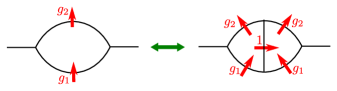
There are two main approaches to thinking about topological response. The first is a bottom-up approach where one starts with a Hamiltonian in a lattice model and one attempts to work out all the topological excitations. For example in 2+1D, one has anyons and symmetry fluxes and one can ask about how they interact. This is tabulated mathematically in a -crossed braided fusion category Etingof et al. (2009); Barkeshli et al. (2014) and one can try to work out a classification of these objects or at least find some interesting examples and then look for lattice realizations.
The second approach is a top-down one where one first assumes the existence of a low energy and large system size (”IR”) limit of the gapped system. This is a topological quantum field theory (TQFT) of some sort and one can just try to guess what it is from the microscopic symmetries, entanglement structure (short-range vs. long-range), and so on. One can make a bold statement that all possible IR limits are of a certain type of TQFT and then try to classify all of those. Despite its obvious lack of rigor, this approach has proven successful.
One reason for this is that it is often possible to bridge the two perspectives. For example, a -SPT can be understood in terms of an effective action Dijkgraaf and Witten (1990); Chen et al. (2013) leading ultimately to a TQFT. But considering the fusion of symmetry fluxes also leads to an element of through a higher associator of symmetry fluxes (in -D, it is the F symbol). These are equivalent under the isomorphism (see Appendix A for more explanation of this isomorphism). In general, defects such as anyons and symmetry fluxes can be described in the TQFT framework through the language of “extended TQFT”.
Let us now discuss how these methods can be extended to the case of spatial symmetries.
IV.1 Flux fusion and braiding for SET phases in (2+1)-D with spatial symmetry
If we want to classify symmetry-enriched phases in (2+1)-D phases we can consider the “bottom-up” approach of Ref. Barkeshli et al., 2014. There, one has a topological phase with an internal symmetry , and one envisages coupling to a classical background gauge field. In particular, one can consider gauge-field configurations in which the gauge fluxes are localized to a discrete set of points. One can then consider the algebraic structure of braiding and fusion of such gauge fluxes, which is an extension of the braiding and fusion of the intrinsic excitations (anyons) that exist without symmetry. This structure is argued to be described by a mathematical object called a “G-crossed braided tensor category”. For a crystalline topological liquid on Euclidean space, we expect that the equivalence between crystalline gauge fields and -connections allows the arguments to carry over without significant change. (We will leave a detailed derivation for future work.) On non-contractible spaces, presumably a generalization of the arguments of Ref. Barkeshli et al., 2014 should be possible, but we will not explore this.
IV.2 Topological Response as Effective Action
Another way to compute topological response, which does not involve braiding or fusing fluxes is by computing twisted partition functions. That is, given a background gauge field (ordinary or crystalline) on a spacetime , we can compute the partition function of and compare it to the untwisted partition function . The assumption is that
tends to a complex number of modulus 1 in the limit that becomes very large compared to the correlation length. In favorable situations, such as a crystalline topological liquid, the limiting phase is a topological invariant of and its gauge background . We call this the topological response of our system to and its log the effective action for the gauge background . In some cases, like , can be interpreted as some kind of “twisted trace” of symmetry operators, as we soon discuss. In general there is such an interpretation but it involves topology-changing operators Baez and Dolan (1995). 777Indeed, on a general spacetime, a generic choice of time direction defines a Morse function and a foliation of spacetime by spatial slices. At critical points of this Morse function, the spatial slice is singular and we have a topology changing operator that gets us from the Hilbert space just before the critical point to the Hilbert space just after. These are all handle attachments and can be thought of as generalized flux fusion processes.. What is most important for classification of phases is that it is a number that captures some (or all) of the data in a “spatially-dependent TQFT”, which we introduce in Section V as the mathematical way to describe a “crystalline topological liquid” phase of matter.
For internal symmetries of bosonic systems, we know that in this case, the limiting ratio can be written
| (6) |
where is a gauge-invariant top form made out of the gauge field. In the case of a crystalline gauge field , we will also assume that the topological response is an exponentiated integral:
| (7) |
where is a top form on made of the twisting field which classifies the cover and the map , used to pull back densities from . In the case that is purely internal, plays the role of in (6).
As discussed in Ref Dijkgraaf and Witten, 1990, responses of the form (6) are the same thing as cocycles in group cohomology, defined as cohomology of the classifying space 888Actually we should use only measurable cohomology or use different coefficients in a different degree: . We discuss this subtlety in Appendix A., where is the dimension of spacetime . This reproduces the classification of internal symmetry bosonic SPTs in Ref Chen et al., 2013. To construct the effective action of , we use the fact that the gauge field itself is the same as a map , and given a -cocycle on , we can pull it back along this map to get over .
Analogously, we can think of our crystalline gauge field as a map (see Appendix E) and take any form in , pull it back along this map to to get a and integrate it (see Appendix G). We just need to be a little careful with coefficients. We intend to integrate over , but if contains orientation-reversing elements like mirror and glide reflections (or time reversal), then may likely be unorientable. Integration on an unorientable is done by choosing a local orientation: orienting away from some hypersurface and performing the integration on with its orientation. To ensure the integral does not depend on this local orientation, we need our top form to switch sign with the local orientation is reversed. Mathwise, this means that should live in cohomology with twisted coefficients . Luckily, if is orientable, then the unorientability of is entirely due to orientation-reversing elements of , so if we use twisted cohomology where orientation-reversing elements of act on by , then the coefficients will pull back properly. This cohomology group is well known in algebraic topology as the equivariant cohomology of , and is written
Another subtlety comes from considering the identity map as a crystalline gauge field. Any non-trivial topological response to the identity cover is equivalent to a shift of all the partition functions by a phase. We may as well consider only the subgroup of all equivariant cohomology classes which pulled back along the identity map are trivial. This is called reduced cohomology and is denoted with a tilde .
Summarizing (and recalling the subtlety about replacing increasing the degree by 1, as discussed in Appendix A ), we find:
Theorem 2.
Homotopy-invariant effective actions in spacetime dimensions for crystalline gauge fields which may be written as integrals over are in correspondence with “twisted reduced equivariant cohomology”:
In the following section, we will give examples of crystalline SPT states and how to compute the topological response as a class in equivariant cohomology.
Finally, even though these are all the effective actions, from what we’ve learned in the case with time reversal symmetryKapustin (2014) and consideration of thermal Hall response, we know these are very unlikely to be all the phases. There are some criteria, like homotopy invariance, that pick out these phases based on their effective action, but we don’t know a microscopic characterization of which phases come from group cohomology and which phases are from the beyond. We say “bosonic” because we have learned the importance of including spin structure in a careful way Kapustin et al. (2015). We discuss the relationship between topological actions and phases in Appendix A.
IV.3 Examples of Topological Response
Let us explain in some examples how the topological response (7) manifests itself physically and how it can be computed starting from an SPT state. These examples were constructed using the techniques in Appendix F.
IV.3.1 Reflection SPT in 1+1D
We consider a system of spin-’s lying along the -axis at integer coordinates . We will use the basis for these spins and consider the state
There is no reflection-symmetric perturbation (keeping the gap) which can take that central minus sign to a plus. This is because it can be understood as an odd charge for an internal symmetry induced by reflection at the reflection center. This odd charge is the signature of this SPT phase. Let us see how to compute it as a topological response.
Observe that this odd charge can be detected using a trace
| (8) |
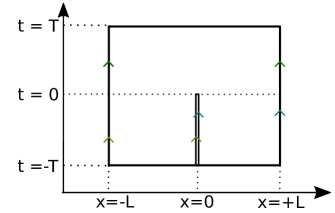
where is a gapped Hamiltonian with ground state as above and is the reflection operator. Traces are computed by path integrals with a periodic time coordinate. The insertion of means that as we traverse this periodic time, we come home reflected. This means that the geometry of the spacetime whose path integral computes this trace is a Möbius strip.
We can represent this geometry as a crystalline gauge field over
the usual domain for background gauge fields used to compute twisted traces. We write the Möbius strip
We get a continuous map
where
There is no continuous lift of this map to , so we insert a branch cut along in . This defines a covering space
with covering map defined by
This has a map defined by
We summarize with a diagram (cf. Defn (2))
| (9) |
The trace (8) is therefore interpreted as a topological response to this crystalline gauge field is a la (7) and we would like to write it in the form for some , where is our double cover interpreted as a gauge field which tells us where the branch cuts are. It turns out there is a unique non-trivial class and indeed if we compute (with particular boundary conditions)
we reproduce the trace (8).
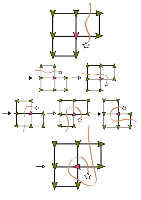
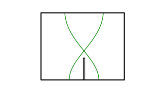
Before we move on to richer examples, let us make some comments for the mathematically inclined on the evaluation of this integral. To get the claimed answer, we used the one-point-compactification of , where we add a single point at infinity, collapsing the boundary to a point. The one-point-compactification of is the projective plane and the usual integral . There is, however, no rigid crystalline gauge field over with since is noncompact. However, if we impose -symmetric, time independent boundary conditions on our crystal, then our cylindrical spacetime gets each end collapsed to a point and becomes a sphere. The reflection group continues to act on this sphere and there is a rigid crystalline gauge field with over .
In computing more complicated examples of this same SPT phase (examples which are not already disentangled), indeed one finds it necessary to choose some boundary conditions in (8) to get a nonzero trace. What if we use periodic boundary conditions? In that case, there is always a reflection center at , and periodicity implies that the reflection center will also carry an odd charge. Therefore, the trace with periodic boundary conditions will receive a contribution from both reflection centers and be . We can see this with our crystalline gauge fields. Indeed, with periodic boundary conditions spacetime becomes a torus and if we insert a reflection twist in the time direction we obtain as a Klein bottle. We identify with the orientation class in and for this class , as expected! On the other hand, one can use Möbius bands centered at either reflection center to see the odd charge at each one. Gluing them along their overlap gives us the Klein bottle again and the partition functions multiply999This is a form of cobordism invariance.. We will see this in more detail in the following example.
IV.3.2 Reflection and Translation in 1+1D
Next we consider a one-dimensional system with a translation and a reflection symmetry. In particular, the state
This state is symmetric under reflection around : , and also under reflection around : . The product is a translation by two units. In the language of the previous example, even sites carry even charges and odd sites carry odd charges. These charges are detected by computing traces
The spacetime geometries of the two traces correspond to two different crystalline gauge backgrounds over . Depending on whether we twist by or , our test manifold is a Möbius band centered over or .
Because we have a translation symmetry, we can also consider a trace in periodic space. If the length of the spatial circle is an odd number of unit cells (for a total length ), then every reflection symmetry passes through an odd and an even site, so all the traces
| (10) |
The spacetime geometry of this trace is a torus with a reflection twist as we go around the time circle, ie. a Klein bottle.
We can describe this trace as topological response to a crystalline gauge background over . We will need to insert branch cuts along both cycles of the Klein bottle . Along the spatial direction, this because we are trying to map . If we coordinatize using , we can consider the map with a branch cut from to where we translate by . Denoting the compatible twisting for translations by , a gauge field on , we therefore have around the spatial cycle. As before, we also have to twist around the time direction by a reflection, say . If we denote by the corresponding compatible twisting, a gauge field on , then we have (mod 2) around the time cycle. Summarizing, we have
| (11) |
We wish to write the trace (10) as a topological response (7) of the form
There are two choices that work, namely
On the other hand, because of the term in , the second describes a non-trivial response to a Möbius band centered over 0. We have argued that the partition function in this background computes the sign of the trace of , which for our SPT state above is positive. Therefore, our state must correspond to the class .
Let us show as a consistency check that this cocycle correctly produces the negative trace over . Using the formula , we see that the Möbius strip over has the twisting (mod 2). Then adding the proper boundary conditions we indeed find
Note that the same caveats about this integral and boundary conditions on the trace we discussed in the previous example apply.
From what we have computed so far, we see that corresponds to having odd charges on even sites and even charges on odd sites and corresponds to having an odd charge on every site, the simplest translation-symmetric extension of our state in the previous example.
IV.3.3 Rotation SPT in 2+1D
Now we consider another simple system, this time on the square lattice with a rotation symmetry . This system has an odd charge, eg. at the rotation center and is a symmetric product state elsewhere. As with the reflection examples, we can see the odd charge at the rotation center using a trace:
The geometry of this trace is a mapping cylinder where we transform by as we go around the circle. The unique non-trivial effective action indeed has
so this is our phase.101010If we use -symmetric, time independent boundary conditions in our trace, corresponding to the one point compactification of , we get real projective 3-space .
The equivalent internal -symmetry SPT is well known to be characterized by flux fusion: two fluxes fuse to an odd charge. This can be easily read off from the Chern-Simons form of its effective action , where is the (ordinary) background gauge field. Indeed, if we read as the density of fluxes, we can read the effective action as a source term for saying precisely that fluxes carry odd charge.
The crystalline equivalent has the same form, so can we read it in the same way? It turns out we can if we identify a gauge flux with the disclination and use the careful definition we gave in II.1. We expect to find a half charge of the disclination, so we will rotate it twice by 180 degrees and see if we pick up a minus sign. As shown in Fig 5, indeed we do.
Note that for an internal symmetry (it’s less clear how it would work for a spatial symmetry), we can promote the gauge field to a dynamical quantum variable and then the gauge fluxes become deconfined excitations with semionic statistics Levin and Gu (2012). A semion has a topological spin (phase picked up under rotation) of , One might ask how this is consistent with the above statement that the symmetry defect picks up a phase of of under two 180 degree rotations. However, we note that this is a rotation in , whereas the rotation that defines topological spin does not take place in but rather in .
IV.3.4 Crystalline Topological Insulators
Now let us discuss 3+1D phases protected by time reversal symmetry or reflection symmetry and a rotation symmetry (typically or , odd has no nontrivial phase). For bosons, these have a classification, with topological response resembling a topological term
where is the twist of the crystalline gauge background. These phases are interesting because this topological term is only non-zero on non-orientable manifolds.111111Indeed, the term may be written , and for all orientable 4-manifolds. This is where time reversal or reflection symmetry comes in. We will consider the reflection symmetry example, which acts across the x-y plane: . We will combine this with a subgroup of , which we may write , while . The combined symmetry is a “parity” symmetry:
Our topological response will be a trace of . To describe this as a path integral, we begin with a cube and glue to with a -twist. Then we choose -symmetric, -independent boundary conditions at . The resulting path integral is over a spacetime , with the generator of . We therefore expect for these special states the topological response
Let us give an example of a state with this topological response. We can actually obtain it from dimensional induction from our symmetric state we discussed above. We place this state along the x-y plane. It is pinned there by the reflection symmetry across that plane. The above trace reduces to a trace of the rotation symmetry on this state, which we have computed sees an odd charge at the rotation center, yielding .
IV.3.5 Sewing Together a Pair of Pants and Internal Symmetry SPT
So far we have discussed how to consider 1+1D twisted traces as crystalline backgrounds over either or in the case that translation is an explicit symmetry. Other partition functions of interest must be computed on higher genus surfaces and a basic building block of these is the pair of pants. Indeed, every orientable closed surface is glued together from discs and pairs of pants. Physically, the path integral over the pair of pants computes a sort of fusion process from to . Let us discuss how the pair of pants is realized as a crystalline gauge background over in a system with a unit translation symmetry .
We construct starting with mapping by inclusion into with a cut along the negative axis from to which doubles the axis into for . We glue the side to and the side of the branch cut to also with . For , we glue to . This gives the topology of the pair of pants. We build a crystalline gauge field by mapping the open domain into by inclusion. We extend this to a -twisted map on all of by inserting branch cuts so that , is glued to , with a twist and , is glued to , with a twist . In terms of the translation twisting field , we thus have on the two “incoming” circles at and on the “outgoing” circle at .
The path integral over the pair of pants is computed by stitching together propagators from the two legs into the waist. These propagators are computed on the cylinder with translation-twisted boundary conditions. For example, on the incoming circle from to , we restrict the Hamiltonian from 121212We assume this Hamiltonian is ultralocal to the lattice. In 1D this means it only couples neighbouring sites. Any finite-range Hamiltonian may be coarse-grained until it satisfies this., and use boundary conditions so that in the product state basis of the on-site Hilbert space , we restrict to the subspace spanned by product states such that the state at is the same as applied to the state at . Translation symmetry ensures that the Hamiltonian preserves this subspace. We compute as an operator from this subspace to . We do the same for the other incoming circle, as an operator landing in . Then we concatenate the two states and project so that the parts agree. Then we are in the subspace of where the part agrees with applied to the part. This is the Hilbert space of the outgoing circle and we can apply on this subspace to obtain the complete pair-of-pants operator from the Hilbert space of the two incoming circles to the Hilbert space of the big outgoing circle.
If we also have an internal symmetry with associated background gauge field , then we can also have twists around these circles encoded in the crystalline gauge background. We denote the twists around the two incoming circles as and around the outgoing circle as . We find that for continuity they must satisfy . We can imagine this is describing a -flux fusion process occurring inside the pair of pants (see FIG. 6. If we choose representative ground states in each sector , the path integral over (topological response (7) with boundary conditions) will be some phase . The crystalline topological liquid assumption implies that if we glue two such pairs of pants together in two different ways, we get equal response, at least in the large limit. This implies that is a group 2-cocycle, encoding the possibility of projective flux fusion. On the other hand, since the phases of our states are unphysical, if we rephase them each , then changes at most by an exact cocycle, so is well defined in group cohomology.
Let us show how this is computed in an example. We consider a very simple symmetric SPT. There are two associated on-site degrees of freedom we denote . We consider the state
The sum is over all labelings of vertices by a pair and the relative phase factor is the number of edges where (mod 2) and (mod 2). The unit translation symmetry is manifest. Less manifest but still a symmetry is the which acts by shifting the respective variables by a global constant. It can be seen by writing
which is invariant under a constant shift and invariant up to boundary terms under .
We must determine the propagator for which this state is the unique ground state. This can be done using tensor network techniques or in this case merely by inspection. We find this state is computed by the path integral over a strip with fixed boundary conditions and free boundary conditions at , using the path integral weight which is to the number of intersection points between and domain walls.
Now for each , we choose a gauge-fixed reference state for the twisted ground state on . This just means we have to decide where the domain walls go. Let’s agree there is at most one domain wall for at and one for at , where the circle is coordinatized by . Then we see all the pairs of pants have trivial phase factor except for the one where the left incoming circle has twist and the right has twist. In this case, the domain walls have to cross (see FIG. 7) so we get a phase . This gives us a function which turns out to be a group 2-cocycle and classifies the nonabelian extension
where is the dihedral group of the square. Extending coefficients to we get the corresponding SPT cocycle . A similar construction of a translation-symmetric state can be made for any -SPT phase.
IV.3.6 Weak SPTs and Lieb-Schultz-Mattis
Now we consider a 2+1D system with internal symmetry and unit translation symmetry in one direction, say . We fix a 1+1D SPT and consider infinitely many copies of this SPT laid side-by-side along . The edge of this system has a projective symmetry per unit cell. We would like to assemble a crystalline gauge background that distinguishes the bulk from the trivial phase. This way, we derive the Lieb-Schultz-Mattis (LSM) theorem as the anomalous edge constraint of this crystalline SPT.
As we discussed, any 1+1D SPT cocycle is detected using the pair of pants (FIG. 6), interpreted as a projective fusion of fluxes. In our case, this flux threads a circle in the -direction, so we must assume there is also a symmetry or at least an emergent one that we can use to roll up the system in that direction. There are various ways to make such a construction. Given a -SPT state
where is some 1-form density depending on (compare previous example)131313This state is in SPT phase iff for all . It is called the first descendant of . See Kapustin and Thorngren (2013), we can write the layered SPT state as
where integrates to 1 across the -direction of any unit cell. This is equivalent to
We can use this to write a state on a torus as
where is the twisting around with the length of and is the twisting around , and is a 1-form density encoding and its coupling to the background gauge field 141414This density will satisfy .. There is a gauge where across each unit cell in the direction. This most closely matches our above, with copies of arranged around the circle . In a gauge with a single branch cut, all copies are piled up at the branch cut.
We see that the proper crystalline gauge background for computing is given by taking (the size of ) coprime to the order of and assembling the pair of pants using the remaining coordinates . With incoming twists , one can compute using the state above the topological response . Essentially this crystalline gauge background is a kind of compactification along . Of course, since we are already in the topological limit, this need not be small. Its size need only be coprime to the order of . If is finite, then it suffices to be coprime to the order of .
Generalizing to the case where the -dimensional unit cell carries the projective representation with 2-cocycle , the topological response is
where are the twists corresponding to the unit translation in the th lattice coordinate. To check for this topological response, we can take our test spacetime to be a -torus (of size coprime to the order of or ) times a pair of pants with -twists.
V Spatially-dependent TQFTs
Here, we will explain our proposal for the description of the low-energy limit of a crystalline topological phase in terms of a TQFT. In this setting, our results, such as the crystalline equivalence principle, and the fact that the low-energy limit can be coupled to an arbitrary crystalline gauge field, can be proven mathematically. We will focus here on the physical motivations; however, we give enough detail that the full mathematically rigorous treatment should be apparent to TQFT experts.
Recall that the starting point is that a phase of matter should have a spatially-dependent “topological limit”, which we expect to be described by a spatially-dependent TQFT. Indeed, we define
Definition 4.
A -dimensional spatially-dependent TQFT on a space is a continuous map , where is the space of all -dimensional TQFTs.
Now, what exactly do we mean by “space of all TQFTs”? Familiar notions of TQFTs (at least in 2+1D) look quite rigid, suggesting that any such space would be discrete. However, we want to argue that there is a natural way to think about TQFTs as living in a richer topological space . First of all, we note that for classifying phases of matter it will not be necessary to specify exactly, only up to homotopy equivalence. Let us discuss a physical motivation for the homotopy type of .
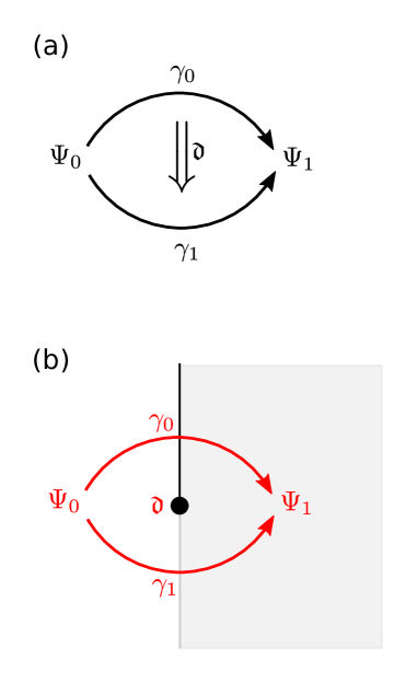
Generally, specifying the homotopy type of a topological space involves identifying points, paths between points, deformations between paths, and so on. The idea is that the structure of should represent features of ground states of quantum lattice models. Thus, the points in should correspond to ground states of quantum lattice models; the paths in should correspond to continuous paths of ground states of quantum lattice models; and so on. There is another way to interpret these statements. A path in the space of ground states of quantum lattice models can also be implemented spatially, giving rise to an interface of codimension 1. Similarly, deformations between paths give rise to interfaces of codimension 2 between interfaces of codimension 1, and so on. (See Figure 8).
Roughly, therefore, the idea is that should have the homotopy type of a cell complex with vertices labeled by -dimensional TQFTs . Edges are labeled by invertible -dimensional topological defects between and . 2-Cells with are labeled by invertible -dimensional junctions between the defects . This continues all the way down to 0-dimensional defects, which for topological field theories with a unique ground state on a sphere is a copy of the complex numbers. 151515Note that if two topological theories share an invertible topological defect, it means they are isomorphic, so in a formulation of TQFT up to isomorphism, eg. modular tensor category, each component of will have a single vertex, perhaps with many other cells attached to it. In a state sum or tensor network formulation, on the other hand, there could be lots of state sums giving rise to the same TQFT with invertible MPO defects between themWilliamson (2016). In Etingof et al. (2009), this space was considered for in the tensor category framework and was referred to as the Brauer-Picard 3-groupoid.
A version of the bulk-boundary correspondence says that the set of boundary conditions and boundary operators determines the bulk topological field theory (see Kapustin (2010) for some perspective on this in general dimensions and Kapustin and Saulina (2011); Fuchs et al. (2013); Henriques (2015) in 2+1D especially). For theories admitting gapped (therefore topological in the IR) boundary conditions, this is the Baez-Dolan-Lurie cobordism theorem (sometimes “hypothesis”) Baez and Dolan (1995); Lurie (2009), which characterizes possible boundary data as special objects in a -category . This characterization can be used to construct in a mathematically precise way. (Specifically, it is a space whose homotopy type is described by the core of the category ).
Let us now consider the effect of symmetries. There is a natural way to define a -action on a TQFT. From the Baez-Dolan-Lurie framework, one can show that a TQFT with symmetry is equivalent to TQFT coupled to a background gauge field. What we mean by the latter is the following. A -dimensional TQFT assigns topological invariants to manifolds; for example, it assigns complex numbers (the partition function) to -dimensional manifolds, and finite-dimensional Hilbert spaces (the state space) to -dimensional manifolds. A -dimensional TQFT coupled to a background gauge field assigns invariants to -manifolds: manifolds decorated with gauge fields. Physically, this is supposed to describe response the topological response of the system to background gauge fields. We want to extend this result to systems with spatial symmetries.
Let us first review the case of a TQFT with an internal unitary -action. Indeed, we define:
Definition 5.
A action on a TQFT is a collection of isomorphisms for each , with consistency data.
In fact, in the Baez-Dolan-Lurie framework discussed above, isomorphisms are just paths in the space . These have the interpretation of defects of codimension 1. In fact, these are just symmetry twist branch cuts (e.g. see Ref. Barkeshli et al. (2014)), such that particles moving through them get acted upon by the symmetry . What we mean by “consistency data” is that the implementation of the relations of are also data in the -action (see for instance Kapustin and Thorngren (2014a)). This data describes the codimension 2 junctions where domain walls fuse, the codimension 3 singularities where two junctions slide past each other, and so on. In fact, a more succinct way to formulate this definition is that a (anomaly-free, see below) TQFT with symmetry is a continuous map . The statement about equivalence between TQFTs with -action and TQFTs coupled to background gauge field then follows from the following general consequence of the Baez-Dolan-Lurie framework (see Thm 2.4.18 of Lurie (2009)):
Lemma 1.
For any space , a continuous map is equivalent to a TQFT for manifolds equipped with maps into .
Indeed, we set and note that maps into are the same as gauge fields.
Finally, we are ready to consider the general case of a spatially-dependent TQFT with a spatial symmetry . We define:
Definition 6.
A -dimensional spatially-dependent TQFT with symmetry on a space is an action of the group on along with a -equivariant map , meaning for all and we have a choice of isomorphism
| (12) |
(with consistency data).
Note that the isomorphisms should be taken to be unitary or anti-unitary for orientation-preserving or orientation-reversing symmetries respectively.
Once all the appropriate consistency data has been taken into account, we find that a spatially-dependent TQFT with an orientation-preserving spatial symmetry corresponds to a map from the homotopy quotient (discussed in section II.4 and appendix E) into . (We will discuss the orientation-reversing case later). Applying Lemma 1, we find
Theorem 3.
A -dimensional spatially-dependent TQFT on with symmetry is equivalent to a TQFT for -manifolds equipped with a (homotopy class of) map , where is the homotopy quotient we have discussed in section II.4.
This statement suggests that we can consider any map as a crystalline gauge background, whereas in section II.1 we only showed how to couple a Hamiltonian to a rigid crystalline gauge background. Indeed, spatially-dependent TQFT mathematically formalizes our notion of smooth states in section II.2 and appendix D. Further, restricting to the case that is contractible, is homotopy equivalent to , so we find the same classification whether acts internally or on .
V.1 Spatially-dependent TQFTs for orientation-reversing symmetries and fermions
Let us now discuss how to extend the above results to systems with orientation-reversing symmetries and/or fermions. First we need to be more specific about the nature of the TQFTs we are discussing. TQFTs come in different flavors (framed TQFTs, spin TQFTs, and so on), depending on what structures we impose on the manifolds to which it assigns invariants. For bosonic systems with orientation-preserving symmetries, the natural choices are TQFTs for either framed manifolds or oriented manifolds. Choosing the latter amounts to assuming that the low-energy limit of our physical system has an emergent Lorentz symmetry, which becomes an Euclidean symmetry after Wick rotating to Euclidean spacetime)161616This is because, in the Baez-Dolan-Lurie framework, one can show that oriented TQFTs arise from an action of on the space of framed TQFTs. See Corollary 2.4.10 of Lurie (2009).. Henceforth, we will always assume that such an emergent Lorentz symmetry is present, though we do not know how to justify this microscopically.
The situation gets interesting when there is also the microscopic symmetry. Indeed, besides the simplest possibility of a total symmetry, there is also the possibility that acts on or there is some kind of extension. The former happens especially when contains orientation-reversing symmetries. Let us suppose is orientable. Whether preserves or reverses the orientation of describes a group homomorphism . We expect this to act non-trivially on any emergent symmetry generators so that the total symmetry algebra contains .
Let us see this in a simple example, a glide reflection acting on , . We assume that the infrared limit of such a system will be a field theory of a map . As we have discussed, in the case of group actions without special Wyckoff positions (ie. free actions), the homotopy quotient is equivalent to the ordinary quotient , which in this case is a Möbius band (cross the time coordinate). Our claim is that the continuum limit of this system is a “sigma model”, a 2+1D field theory whose only field is a map . What does it take to write an action for this field theory? The usual sigma model action is the volume of the image of , or
where is a volume form on . The issue is that is not orientable, so the volume form cannot be globally defined. Rather it is a 3-form valued in the orientation line bundle , a real line bundle whose sections switch sign when one follows them around the Möbius band. When we pull back the volume form using , the result is a 3-form valued in . In order to integrate this over , the fundamental class must be also valued in . This occurs iff is isomorphic to the orientation line of . This means that if a 1-cycle of encircles the Möbius band, must be unorientable around that cycle. In the gauge theory description, these are the cycles with odd holonomy, which have non-trivial image under the map we have just discussed. We discuss more about sigma models in Section VII.3.
Another way of saying this, which makes sense in general, is that the tangent bundle of gives rise to a bundle over , and rather than being oriented, the orientation is on . This sort of phenomenon is familiar also in the internal symmetry case, and is especially crucial once fermions are considered Kapustin et al. (2015). For this reason, we expect this to be the form emergent Lorentz symmetry takes in crystalline topological liquids. 171717In the case that there is no emergent Lorentz symmetry and must be framed, the orientation-reversing elements will act on the framing, and so it must be considered a framing not of but rather .
To proceed, let us recall more from the case where acts trivially on Kapustin et al. (2015). The data that specifies the group of fermionic SPT phases is a map encoding which elements of are time-reversing elements, and also a group extension encoding how the relations of may be extended by fermion parity . As the notation suggests, both may be encoded in a bundle over , with and . We call this the characteristic bundle. It may be interpreted in field theory as the representation of the fermion bilinears. The low energy limit of a gapped theory with such a symmetry is expected to be a theory defined on manifolds with a gauge field and a spin structure on . The cobordism group of such manifolds only depends on through and . Since is itself a bundle over , any characteristic bundle also defines a bundle over . This leads us to:
Theorem 4.
A bosonic (fermionic) crystalline topological liquid with microscopic symmetry , characteristic bundle , and emergent Lorentz symmetry has a topological limit defined on manifolds with a map and an orientation (spin structure) on .
As an example, if acts on by rotation of space, is a plane bundle over . In terms of the tautological line bundle (corresponding to the sign representation), this bundle is . One computes and , which generates , corresponding to the extension of . In the absence of any nontrivial , this means that the rotation squares to the fermion parity. This is what we typically expect of rotations of fermions.
On the other hand, if there is an internal symmetry squaring to the fermion parity, such as a charge conjugation (unitary) symmetry, , then we can combine this with the rotation symmetry to obtain a unitary symmetry squaring to 1. By the crystalline equivalence principle, or by Thm 3, we expect such phases to give rise to topological field theories for manifolds with a spin structure on and a gauge field . Let’s see how the conjecture above encodes this. As explained in Kapustin et al. (2015), a unitary representation with corresponds to the characteristic bundle over (recall is the bundle of the sign representation ). Since of the rotation symmetry was trivial, this is also of the composite symmetry. The conjecture above says that we will obtain in the infrared a theory of manifolds with and a spin structure on . It turns out has both and . This means that we may choose a spin structure on this bundle and thereby form an isomorphism between spin structures on and spin structures on and there is no contradiction.
Given this conjecture, we can state the crystalline equivalence principle more precisely:
Theorem 5.
If , then any action on defines a vector bundle over . The action on internal degrees of freedom defines another bundle over . SETs with this sort of crystalline symmetry are isomorphic to SETs with internal symmetry and characteristic bundle .
The most important aspect of this theorem is the identification of orientation-reversing symmetries like reflection with anti-unitary symmetries like time-reversal in the classification of topological phases. Indeed, for bosonic systems with , all that matters of is the determinant of the representation (ie. ), which is multiplicative over direct sum. Thus, a time reversal symmetry, which has and trivial, is equivalent to a reflection symmetry, which has and trivial.
An important caveat about this in fermionic systems is that reflection with corresponds to . Indeed, the former leads us to consider TQFTs for manifolds with and a spin structure on . This is equivalent to a Pin+ structure on , which in Kapustin et al. (2015); Freed and Hopkins (2016) is what needs to be considered for the classification of phases. This is because our spacetimes are Euclidean, and Wick rotation changes the behavior of orientation reversing symmetries.
V.2 Comments on Anomalies
In the beginning of this section, we made an identification between TQFTs with a symmetry and TQFTs parametrized by . This identification is actually only possible when the symmetry is anomaly free.
0+1D is an instructive example. Such TQFTs describe the ground states of quantum mechanical particles and so the space of 0+1D TQFTs can be described as the space of finite dimensional Hilbert spaces (here is the dimension of the ground state degeneracy). The ground states of a quantum mechanical particle with symmetry are characterized by a unitary representation of . This representation defines a vector bundle over whose fibers can be considered different 0+1D TQFTs, and has a classifying map .
In quantum mechanics, however, there is the possibility that the action on the space of ground states is projective. In 0+1D this counts as an anomaly. In this case, we don’t get a vector bundle over but rather a projective vector bundle. Such a bundle does not have a classifying map . Rather, the anomaly is characterized by a bundle over with fiber , and the anomalous theory can be described as a section of this bundle. For group cohomology anomalies, classifies bundles over with fiber . This defines a bundle by the diagonal map . The story in all dimensions is a direct generalization with no new ingredients, though in practice it is difficult to work out the details Nikolaus et al. (2015); Freed and Teleman (2012).
We expect that there could be an analogous phenomenon for the spatially-dependent TQFTs. That is, we defined a crystalline topological liquid as a system with a topological limit described by a map . However, it could be that there are “anomalous” crystalline topological liquids, characterized by a section of a bundle over with fiber . With symmetries this would become a section of such a bundle over .
The anomaly itself would be characterized by the bundle . The simplest examples would come from ordinary equivariant cohomology , where is the spacetime dimension of the anomalous theory. This suggests a kind of crystalline anomaly in-flow mechanism which would be interesting to study. We leave this to future work.
VI Classification of phases in non-contractible space
As mentioned above in Section II.4, our framework in principle can be applied to the classification of topological phases with spatial symmetries on any space , not just . In this section we discuss a few examples of this classification to indicate the general flavor, and state some general properties. We emphasize that, although our classification can be applied to any space (for example, a compact manifold), our results are only expected to be physically valid when the size of this manifold is much greater than the lattice spacing and the correlation length; otherwise, we cannot define the “topological limit” discussed in Section I which underlies our arguments.
VI.1 Properties of the classification
All these statements are derived from properties of the homotopy quotient discussed in Appendix E.
VI.1.1 Properties that hold in general
The following statements are valid for the classification of crystalline phases in full generality. We let denote the classification of crystalline topological phases with symmetry acting on a space . We let denote the classification of crystalline topological phases with internal symmetry .
-
•
Crystalline Equivalence Principle If , then . For orientation-preserving symmetries, we find an isomorphic classification with those phases protected by an internal unitary symmetry. For orientation-reversing symmetries, we find for example that inversion-symmetric phases have the same classification as time-reversal-symmetric phases.
-
•
Rolling and Unrolling If contains a normal subgroup which acts freely on , then we can quotient by and obtain an equivalent rolled up phase: . We can also unroll a phase along any circular coordinates to get an equivalent phase with a translation symmetry in the unrolled direction, so these classifications are isomorphic. In particular, if is the space group of a crystal, then the translations are a normal subgroup which act freely and we may instead study the point group acting on the quotient torus. This works even for non-symmorphic symmetries, as observed in Ref Hiller, 1986: even if there is no symmetry center, the point group will act on the fundamental torus. However, this residual group can still contain things like glide reflections (and certainly will if we are in a non-symmorphic situation).
VI.1.2 Properties that hold for “in-cohomology” bosonic SPTs
. The following statements hold for the “in-cohomology” bosonic SPTs discussed in Section IV.2, which are classified by the equivariant cohomology .
-
•
No Translation SPTs If acts freely on , eg. translations on , then by rolling up along all the translations we get an equivalent phase on a torus without any symmetries: . In particular, since is a manifold, the reduced cohomology in the top degree is always zero, so there are no non-trivial phases.
-
•
New Internal SPTs Protected by Topology On the other hand, if is an internal symmetry, meaning it doesn’t act on , then . This means . If we require that has no dependence on , we find the usual group cohomology classification for internal symmetry SPTsChen et al. (2013). We see however the possibility for new equivariant cohomology SPT phases which are protected by the topology of as well as symmetry. These all look like lower dimensional SPT phases wrapped perpendicular to non-contractible cycles of .
-
•
Finitely Many Phases in Each Symmetry Class In fact, all phases originate in some element of . We discuss how this works in Appendix G. Because we can roll up our phases to equivalent ones with finite symmetry , the only piece of which can contribute infinite order elements is the piece . Happily, since is -dimensional, this piece always vanishes, so is finite and therefore there are only finitely many phases in each symmetry class .
VI.2 Examples of Phases on Non-contractible Spaces
VI.2.1 Reflection Acting on a Circle and Unrolling
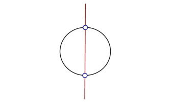
Consider a system on a circle with a reflection symmetry . By arguments of Ref Song et al., 2016, there should be a classification corresponding to the residual charges at the two fixed points (see Figure 9). For our classification, these phases live in . The cohomology groups in the descent sequence (Appendix G) which contribute are
where is the (degree one) generator of cohomology of and is the element of which integrates to over the circle. It is the unique fixed element under the action.
We observe the similarity with and in Section IV.3.2, where we considered a system with a reflection (corresponding to ) and translation (corresponding to ) symmetry. Indeed, taking the quotient of that system by the translation symmetry, we obtain the circle with reflection action. The translation part of the crystalline gauge field becomes the volume form of the quotient . Identifying the topological response, we find that has an odd reflection charge at both fixed points, while has a single odd reflection charge at a fixed point. Which fixed point in particular depends on the choice of cocycle representing and can be traced to the choice of preferred reflection center of the unrolled system. The state with the odd reflection charge at the other fixed point will correspond to the topological response .
VI.2.2 Orientable Actions on Spheres
Another interesting case is when space is a sphere with acting via . The descent tells us that all such phases are a combination of those in , the ordinary SPT phases, and , which correspond to a system whose ground state on has a (abelian) charge with character . These phases are not independent, but are related by the Gysin sequence Hatcher (2002). If we write for the volume form on with unit volume , then the classes in may be written . These classes are not necessarily well-defined on . This is because is no longer necessarily zero, but instead can be
This is the top Stiefel-Whitney class (or often “Euler class”) of the associated bundle over of which is the unit sphere bundle. Physically, this equation says that the “Skyrmion number” is not conserved in the presence of instantons , where is a (2d) time slice and is the crystalline gauge field. The topological response tells us that Skyrmions carry charge so for charge to be conserved we need to satisfy the anomaly vanishing formula . On the other hand one can show that is always injective. We believe this to be related to the fact that one can obtain all SPT phases from sigma models on the sphere Bi et al. (2015) (see also Section VII.3 below). To summarize, the group of phases on sits in an exact sequence
| (13) |
The first map is the inclusion of ordinary SPT phases, the second measures the charge of the ground state on , and the third is the anomaly map.
VII Generalizations
VII.1 Floquet SPTs and gauged Floquet SPTs
The TQFTs defined by our topological actions do not have a preferred axis of time. In a sense there is no difference between a discrete space translation and a discrete time translation. This suggests that all of the crystalline topological phases we have discussed with a discrete spatial translation symmetry can be thought of as Floquet crystalline topological phases Khemani et al. (2016); von Keyserlingk and Sondhi (2016); Else and Nayak (2016); Potter et al. (2016); Roy and Harper (2016a); Po et al. (2016); Potter and Morimoto (2016); Roy and Harper (2016b) which appear in a driven system with time-periodic Hamiltonian , with . (To make sense of this, we should take the space on which the symmetry acts to be space-time rather than just space). We will not, however, attempt to explain how precisely one arrives at a topological action describing such a driven system, nor even what it actually means to “gauge” a discrete time-translation symmetry.
For example, in 1+1D the phases can be interpreted as Floquet phases with internal symmetry. For finite , this is and agrees with the classification in Ref. von Keyserlingk and Sondhi, 2016. The first group represents bulk SPT order and the second group represents a charge being pumped each time step.
We mention that and so there seems to be a topological response analogous to these charge pumping phases but with symmetry . Though it is possible to construct finely tuned models which do this, they all seem to transport some non-trivial quantum information, so we remain skeptical that they exist in real systems.
There are also phases that mix Floquet and crystalline symmetry, for example in 2+1D on with a translation symmetry and a Floquet symmetry there is a phase in . The interpretation is that the system pumps a charge per unit cell per time step on the boundary. This can be rolled up into a Floquet system on a cylinder which pumps a charge per time step to the boundary circle.
It is possible to also pump higher dimensional SPT phases to the boundary. In a sense this is because SPT phases are themselves generalized abelian charges. These phases live in , which is for finite . For example, in 3+1D we are talking about . For connected Lie groups these classify Chern-Simons actions. These correspond to 3+1D phases which pump a Chern-Simons theory to the boundary each time step. For these are integer quantum Hall states.
We pause here to appreciate that if we can build a Floquet system which pumps (internal) SPT phases to the boundary, then we can think about coupling to a dynamical gauge field. Generically, this makes the SPT phase no longer invertible. For example, a trivial SPT in 2+1D becomes the toric code, which is topologically ordered. This does not mean, however, that we pump any non-trivial degrees of freedom to the boundary every time step. Rather, we have a gauge theory at the boundary and at each time step we pump a topological term. For example, the 3+1D Floquet phase with internal which pumps the group cohomology SPT to the boundary each time step has in the gauged picture a gauge theory on the boundary which at one time step is a toric code and at the next is a double semion and then toric code again. It is as though half a charge is pumped to the fluxes and they become semions. If one models this with a Walker-Wang model, then the fluxes on the boundary are themselves the boundaries of strings that reach into the bulk. It is as though these strings are decorated with half (!) the non-trivial 1+1D Floquet SPT, something that pumps half a charge each time step.
Finally, let us note that, according to the “unrolling” principle in Section VI, a TQFT in a space-time with discrete time-translation symmetry is formally equivalent to a TQFT in a space-time with a compactified time dimension. One might wonder how this differs from a system at finite temperature, which also can be interpreted in terms of a compactified time dimension. The difference is that the latter system still has a continuous time-translation symmetry, whereas Floquet systems do not.
VII.2 Fermions and Beyond Group Cohomology
Although we have mainly been talking about bosonic systems, the general framework of our paper is applicable to fermionic systems as well. Indeed, the notion of crystalline gauge field is independent of whether the system is bosonic or fermionic, and in Section V.1 we explained how to define fermionic versions of “spatially dependent TQFTs”. Here we will think some more about fermionic crystalline SPT phases.
We note that this section is not really a “generalization”, since it falls within our general framework. It is, however, a generalization of the equivariant cohomology formulation of bosonic SPT phases discussed in Section IV.2. We can go beyond equivariant cohomology by considering equivariant cobordism. This is where the invariants discussed in Ref Shiozaki et al., 2016 live. The definition of the most general equivariant cobordism is delicate, but by the Crystalline Equivalence Principle, we can assume that fermion phases for spacetime symmetries are like fermion phases for internal symmetries. By what we’ve learned from Ref Kapustin et al., 2015, the data we need to define spin cobordism is a homomorphism telling us which elements of are orientation-reversing and a group extension telling us how is extended by fermion parity. Then there is a corresponding equivariant spin cobordism group . These two classes can be nicely encoded in a single -representation called the characteristic bundle (see Section V). Then we write . These are equivariant cobordism invariants of -manifolds with a spin structure on , where is the gauge field. For example, the ordinary topological insulator in 3+1D lives in where is the fundamental 2d representation of on plus two copies of the sign representation on . This corresponds to the being orientation reversing and squaring to . Details are in Ref Kapustin et al., 2015. It so happens .
Let us give a concrete example of a 2+1D fermionic crystalline SPT with symmetry (not extended by fermion parity), which is related to an internal fermionic SPT which carries a Majorana zero mode at a symmetry flux Kapustin et al. (2015); Tarantino and Fidkowski (2016); Gaiotto and Kapustin (2016); Bhardwaj et al. (2016). This model is very simple. It exists on a square lattice with symmetric Kastelyn orientation and four Majorana operators per site, each associated with one of the 4 edges incident there (see figures). The Kastelyn orientation is used to define a Kitaev-wire type Hamiltonian that dimerizes the Majoranas and will be at least symmetric. One sees that at a disclination, there is a vertex with just three bonds incident, so one Majorana is left unpaired, so in a sense, the disclinations will carry nonabelian statistics.
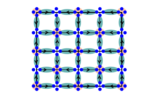
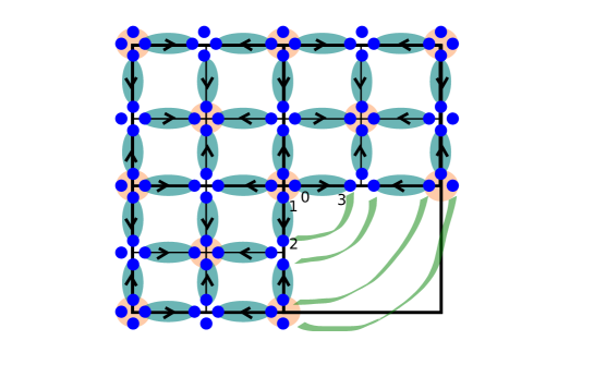
If we add to the ordinary TI a reflection symmetry , then the new cobordism group we need to compute is , where is the sign rep of acting on . This group contains at least a , with the first being the ordinary TI invariant and the second being the invariant of the structure made out of the reflection symmetry. Indeed, a system with a symmetry and a reflection symmetry is a lot like the TI. Indeed, for our classification there is no difference in the group data. As is well known, this has a invariant. So we know these are cobordism invariants, we just have to determine whether they’re non-trivial. From Ref Bahri and Gilkey, 1987, we know that in Pinc+ bordism, and are independent. Further, they each also have a Pin structure, so they define independent classes in . We know from, eg. Ref Kapustin et al., 2015 that the invariant is order 2 on both and and the invariant is order 2 and order 8 on them respectively. This proves that . In particular, since all the free fermion phases are classified by cyclic groups (see Ref. Song and Schnyder, 2016), some of these must be inherently interacting fermionic phases.
We can of course also consider situations where the space group is a non-trivial extension of time reversal (there are 1651 magnetic space groups in 3dLitvin (2013)) and charge symmetries. This gives the possibility of an endless zoo of topological superconductors and insulators, most of which will likely be beyond free fermions!
We can also go beyond cohomology in just bosonic phases. For phases with orientation-reversing symmetries this is very important. As we learned from Ref Kapustin, 2014, we need to consider the unoriented bordism group. If denotes the subgroup of whose symmetries are orientation-preserving, then by the Crystalline Equivalence Principle the most general bosonic phases on spacetime will be classified by . For these we are allowed to use the Stiefel-Whitney classes in our topological terms Kapustin (2014); Thorngren (2015).
VII.3 Coupling a QFT to TQFT and sigma models
One very important use of (invertible) topological field theories besides classifying (short-range-entangled) gapped Hamiltonians is in forming twisted versions of dynamical theories. Indeed, the partition function of a quantum field theory often splits into a sum over topological sectors
A usual example is when is a gauge theory and is the topological class of the gauge bundle. In this situation, the theory may be twisted by an SPT to obtain a new theory
In Aharony et al. (2013); Kapustin and Thorngren (2014b); Kapustin and Seiberg (2014) it was described how these twists change the categories of line and surface operators in the gauge theory. In Scaffidi et al. (2017) this technique was employed to symmetry breaking critical points to define interesting CFTs.
Another example of a class of theories with topological sectors are the “sigma models.” A sigma model on a -dimensional spacetime has an -dimensional target space and counts among its degrees of freedom a map . The partition function splits as a sum over homotopy classes of this map. When , such models are typically gapless and depend on a choice of metric on . Indeed, a typical Lagrangian is proportional to the volume of . However, it is also possible to study topological sigma models, which depend only on the homotopy class of . An invertible such theory, ie. one whose partition function is just a phase can be used to define the twisted sigma model partition function
where denotes a homotopy class of map and is the action of the dynamical sigma model (and we have suppressed other degrees of freedom).
The theories are among the ones we have already studied in the case . We have described how those which can be writted as an exponentiated integral of a local density come from . However, in light of the previous section, we should expect that to account for all possible twists, we should use the cobordism of instead: either in the bosonic case or in the fermionic case.
For example, if and , there is a possibility of topological terms for a fermionic system, classified by , while for bosons there is no non-trivial topological term. This topological term was discussed in Abanov and Wiegmann (2000); Freed et al. (2017) and references therein. When , it equals minus one to the Hopf index of the map .
It is interesting to include symmetry in the picture as well. Suppose first that is an internal symmetry, in that it doesn’t act on the spacetime , but does act on the target space . When we couple to a background -gauge field, becomes a map to . Recall this is a fiber bundle over with fiber . The gauged model will be topological in the directions but may be dynamical in the fiber direction. Anyway, it can be twisted by a topological sigma model with target . These are the theories we have studied, and are classified by in the bosonic case and in the fermionic case.181818There is also the possibility of adding a characteristic bundle to modify the tangent structures involved, à la Section V.1.
For example, if , and , with acting by the antipodal map of , and . This can be understood beginning from the ungauged model, which has an integer topological invariant, the degree of the map . The only -symmetric values of the corresponding angle are , corresponding to this cohomology. The special point coincides with the spin-1/2 Haldane chainHaldane (1983).
VIII Beyond crystalline topological liquids
In section V, we discussed a picture of a limit of crystalline topological liquids which looks like cells occupied by topological orders and boundaries between cells carrying invertible topological defects. It is interesting to consider the generalization where these domain defects are not necessarily invertible. For instance, a chiral Chern-Simons theory forms a topological defect between a Walker-Wang model and a trivial vacuum. The groundstate degeneracy prevents this defect from being invertible, indeed, its tensor product with its parity-inverse is a non-chiral Chern-Simons theory which carries some ground state degeneracy and therefore is not isomorphic to the trivial defect.
In order to account for the non-invertible of these defects, we will need to co-orient the boundaries between cells of (as well the higher codimension junctions). Along with an orientation of the ambient space(time) , this defines an orientation of all the domain walls, allowing them to support parity-sensitive theories like Chern-Simons. We call a space with a cellular decomposition and co-orientations of all cell junctions a directed space. One can study spatially-dependent TQFTs over a directed space .
A directed space can be most concisely discussed as a sort of category, although this involves passing to the dual cellulation with orientations. For example, a circle with a directed edge can be thought of as a category with one object and an endomorphism for every nonnegative integer. This integer tells how many times one winds around the circle but we can only go one way. For example, if with a preferred time direction, then it would be possible to describe a family of TQFTs which says the system pumps a toric code every time step, since now time evolution need not be invertible. Perhaps such a thing is possible in a system with an emergent arrow of time! We could also have the circular direction be a direction of space and this is a quotient of the stack of toric codes we’ve talked about before. So this exotic phase is not beyond TQFT afterall, but the directed space structure is very important. This tells whether we stack toric codes or the CPT conjugate of toric codes. These edge directions in space might be used to describe “fracton” excitations Vijay et al. (2016); Haah (2011) that can only move in certain directions. Whether more general fracton phases can be encoded this way, we don’t know, but while we suspect it is possible, it is probably not enlightening.
There are some sorts of directed space structures which have already appeared in physics. An important one is the Kastelyn orientation of a surface. These are (relative to a dimer configuration) equivalent to a choice of spin structure. Perhaps spatially-dependent TQFTs on Kastelyn oriented surfaces have something to do with spin TQFTs. One can think about the maximum sort of this structure: a branching structure. It seems that a branching structure plays the role of a framing in the Baez-Dolan-Lurie cobordism theorem. Indeed, it gives one all the proper orientations to decorate the cell structure of with line operators, surface operators, … and co-orient them properly so that they can be consistently fused.
IX Open problems
In this work we have presented a general framework for understanding the classification of interacting topological crystalline phases, for both bosons and fermions. An important question for future work is to understand the physical signatures of these phases.
The classic signature of an SPT phase is the protected gapless modes on the boundary (though in strongly interacting systems the boundary can also spontaneously break the symmetry or be topologically ordered). One would expect similar statements to hold for crystalline SPT phases, but there are some caveats. Firstly, of course, a boundary will in general explicitly break the spatial symmetry down to a subgroup, and one only expects protected modes when the phase is still non-trivial with respect to this subgroup. But even then there are exceptions. For example, an SPT protected in 1-D by inversion symmetry about does not have a protected degeneracy when placed on the interval , even though the entire boundary (comprising two points) is in fact invariant under the symmetry Pollmann et al. (2010). Another example is a phase in 2-D with a rotation symmetry, which can be constructed using the techniques of Ref. Song et al. (2016). A ground state in this phase is equivalent by a local unitary to a product state, with a charge pinned to the origin; therefore, there will not be any non-trivial edge states for any choice of boundary. Thus, it is still an open question to determine what is the criterion which ensures protected boundary modes. A way to answer this would be to extend our spatial symmetry gauging procedure to systems with boundary. This is, however, beyond the scope of the present work.
Another question is the robustness of the topological crystalline phases that we have found to disorder, which explicitly breaks the spatial symmetries. There are some topological crystalline phases which have been argued to be robust to disorder, so long as the spatial symmetry is respected on average Chiu et al. (2016). It would be interesting to determine the general circumstances under which this happens.
Acknowledgements.
We thank M. Barkeshli, P. Bonderson, N. Bultnick, X. Chen, L. Fidkowski, M. Hermele, M. Metlitski, C. Nayak, S. Galatius, B. Ware, D. Williamson and C. von Keyserlingk for helpful discussions. We also thank M. Hermele for drawing our attention to a mistake in a previous version of Table I. RT is supported by an NSF GRFP grant. DVE is supported by the Microsoft Corporation. This work was conducted in part at the Boulder Summer School for Condensed Matter and Material Physics, which is supported by the NSF and the University of Colorado; and at the Kavli Institute for Theoretical Physics, which is supported by NSF grant no. NSF PHY-1125915.Appendix A Topological Terms vs. Topological Phases
Let us discuss Dijkgraaf and Witten’s construction of the topological action in more detail. The important observation is the existence of a classifying space : homotopy classes of gauge fields for discrete internal symmetry group are in one-to-one correspondence with continuous maps from . may be constructed as a quotient where is any contractible space on which acts freely, ie. by translations. and hence are often infinite dimensional, in fact necessarily so if has any torsion. This allows there to be nontrivial SPT phases in infinitely many dimensions. From this definition, one easily verifies that the homotopy class of is determined only by the group . Moreover, the cohomology of the group can be defined to be the cohomology of the classifying space (but see below for some subtleties for non-finite groups) . 191919This correspondence can be used to connect many algebraic facts about groups to topological properties of the classifying space and vice versa. For example, a representation corresponds to a vector bundle over . The characteristic class of this bundle determines whether it is an orientable bundle. The characteristic class determines whether it lifts to a spin representation . Furthermore, computing the cohomology of is often easier than attempting a direct calculation of the group cohomology of .
Given on , we write the action
| (14) |
where is a gauge field on considered as a map and is the pullback of forms. Because has coefficients defined only mod integers, is defined modulo times integers. This is because the physical quantity is really .
For infinite discrete groups, one cannot subsequently sum over the gauge field in the path integral to obtain a gauge theory because there are infinitely many gauge equivalence classes of gauge field. However, it still makes sense to consider these gauge fields as backgrounds, if not dynamical, in which case again the topological terms which can be written as local integrals of just the gauge field are classified by .
An important caveat is that the topological terms in do not necessarily correspond to topological phases. For example, with symmetry in 3+1d one can have a theta angle for the gauge field, but this does not mean there is an entire circle of different topological phases. Instead, the existence of the theta term descends to the existence of the Chern-Simons term in 2+1d, whose coefficients are quantized, as phases of matter should be. The famous relationship is
| (15) |
where is the Chern-Simons form of .
For connected symmetry group like or (and indeed for any group) the proper cohomology to consider actually lives one dimension higher than spacetime and over the integers: . Let us remark that physicists often preferChen et al. (2013) to write the classification as , where denotes the “measurable” or “Borel” group cohomology. This can be proven to be isomorphic to .
For finite , coincides with . The problem is infinite order elements in the homology of with which one can define theta angles. These were encountered in Refs Kapustin, 2014 and Kapustin et al., 2015 and the solution there was to use only the torsion part of homology: and consider maps from that group to : . Since abelian groups always split between their torsion and free part, there is an inclusion of this into but more importantly also into by measuring the winding number of the form, much like in Eq 15. These are the sort of gappable-edge SPT phases encountered in studying finite symmetries. The non-torsion pieces in homology define things like Chern-Simons terms, which are descended from 4d integer characteristic classes like the first Pontryagin class or second Chern class and their corresponding theta terms , . Our belief is that the universal coefficient sequence Hatcher (2002)
| (16) |
encodes a physical short exact sequence with the same functorial and splitting properties
This is discussed also in Ref Kapustin et al., 2015 where the inclusion of infinite order homology elements in shifted degree corresponds to thermal Hall-type gravitational response and Ref Freed and Hopkins, 2016 where it is related to the Baez-Dolan-Lurie cobordism theorem and the Anderson dual of the sphere spectrum, which in topology plays the role of , the Pontryagin dual of .
| Number | Name | Classification |
|---|---|---|
| 1 | 0 | |
| 2 | ||
| 3 | ||
| 4 | 0 | |
| 5 | ||
| 6 | ||
| 7 | 0 | |
| 8 | ||
| 9 | 0 | |
| 10 | ||
| 11 | ||
| 12 | ||
| 13 | ||
| 14 | ||
| 15 | ||
| 16 | ||
| 17 | ||
| 18 | ||
| 19 | 0 | |
| 20 | ||
| 21 | ||
| 22 | ||
| 23 | ||
| 24 | ||
| 25 | ||
| 26 | ||
| 27 | ||
| 28 | ||
| 29 | 0 | |
| 30 | ||
| 31 | ||
| 32 | ||
| 33 | 0 | |
| 34 | ||
| 35 | ||
| 36 | ||
| 37 | ||
| 38 | ||
| 39 |
| Number | Name | Classification |
|---|---|---|
| 40 | ||
| 41 | ||
| 42 | ||
| 43 | ||
| 44 | ||
| 45 | ||
| 46 | ||
| 47 | ||
| 48 | ||
| 49 | ||
| 50 | ||
| 51 | ||
| 52 | ||
| 53 | ||
| 54 | ||
| 55 | ||
| 56 | ||
| 57 | ||
| 58 | ||
| 59 | ||
| 60 | ||
| 61 | ||
| 62 | ||
| 63 | ||
| 64 | ||
| 65 | ||
| 66 | ||
| 67 | ||
| 68 | ||
| 69 | ||
| 70 | ||
| 71 | ||
| 72 | ||
| 73 | ||
| 74 | ||
| 75 | ||
| 76 | 0 | |
| 77 | ||
| 78 | 0 |
| Number | Name | Classification |
|---|---|---|
| 79 | ||
| 80 | ||
| 81 | ||
| 82 | ||
| 83 | ||
| 84 | ||
| 85 | ||
| 86 | ||
| 87 | ||
| 88 | ||
| 89 | ||
| 90 | ||
| 91 | ||
| 92 | ||
| 93 | ||
| 94 | ||
| 95 | ||
| 96 | ||
| 97 | ||
| 98 | ||
| 99 | ||
| 100 | ||
| 101 | ||
| 102 | ||
| 103 | ||
| 104 | ||
| 105 | ||
| 106 | ||
| 107 | ||
| 108 | ||
| 109 | ||
| 110 | ||
| 111 | ||
| 112 | ||
| 113 | ||
| 114 | ||
| 115 | ||
| 116 | ||
| 117 |
| Number | Name | Classification |
|---|---|---|
| 118 | ||
| 119 | ||
| 120 | ||
| 121 | ||
| 122 | ||
| 123 | ||
| 124 | ||
| 125 | ||
| 126 | ||
| 127 | ||
| 128 | ||
| 129 | ||
| 130 | ||
| 131 | ||
| 132 | ||
| 133 | ||
| 134 | ||
| 135 | ||
| 136 | ||
| 137 | ||
| 138 | ||
| 139 | ||
| 140 | ||
| 141 | ||
| 142 | ||
| 143 | ||
| 144 | 0 | |
| 145 | 0 | |
| 146 | ||
| 147 | ||
| 148 | ||
| 149 | ||
| 150 | ||
| 151 | ||
| 152 | ||
| 153 | ||
| 154 | ||
| 155 | ||
| 156 |
| Number | Name | Classification |
|---|---|---|
| 157 | ||
| 158 | 0 | |
| 159 | ||
| 160 | ||
| 161 | 0 | |
| 162 | ||
| 163 | ||
| 164 | ||
| 165 | ||
| 166 | ||
| 167 | ||
| 168 | ||
| 169 | 0 | |
| 170 | 0 | |
| 171 | ||
| 172 | ||
| 173 | ||
| 174 | ||
| 175 | ||
| 176 | ||
| 177 | ||
| 178 | ||
| 179 | ||
| 180 | ||
| 181 | ||
| 182 | ||
| 183 | ||
| 184 | ||
| 185 | ||
| 186 | ||
| 187 | ||
| 188 | ||
| 189 | ||
| 190 | ||
| 191 | ||
| 192 | ||
| 193 | ||
| 194 | ||
| 195 |
| Number | Name | Classification |
|---|---|---|
| 196 | ||
| 197 | ||
| 198 | ||
| 199 | ||
| 200 | ||
| 201 | ||
| 202 | ||
| 203 | ||
| 204 | ||
| 205 | ||
| 206 | ||
| 207 | ||
| 208 | ||
| 209 | ||
| 210 | ||
| 211 | ||
| 212 | ||
| 213 | ||
| 214 | ||
| 215 | ||
| 216 | ||
| 217 | ||
| 218 | ||
| 219 | ||
| 220 | ||
| 221 | ||
| 222 | ||
| 223 | ||
| 224 | ||
| 225 | ||
| 226 | ||
| 227 | ??? | |
| 228 | ??? | |
| 229 | ||
| 230 | ??? |
Appendix B Computing the bosonic classification
A nice feature of our results, at least in the case of bosonic crystalline SPTs (in Euclidean space) is that the classification is readily computable. According to the general discussion of Section IV.2, we see that the classification in space dimensions for a given space group is given by . Computing this object turns out to be within the capabilities of the GAP computer algebra program GAP (2016). We show the results in Table 1 (in the introduction) for the (2+1)-D case and in Table 2 for the (3+1)-D case. There were 3 space groups in (3+1)-D for which the classification took too long to compute and is not shown.
We recall that this classification is expected to be complete in (2+1)-D, and for the Sohncke groups (those not containing any orientation-reversing elements) in (3+1)-D. What about explicit constructions of these phases? Let us fix some element . Suppose that there exists a finite group and a group homomorphism such that is in the image of the map induced by . Then indeed we have an explicit construction of the crystalline SPT correponding to , using the bootstrap argument of Section III (leveraging, for example, the construction of Ref. Chen et al., 2013 for the SPT protected by acting internally). We conjecture that there will always be some such for any element of .
Appendix C Coupling a Hamiltonian to a rigid crystalline gauge field
In this appendix, we explain how to couple a finite range Hamiltonian to a crystalline gauge field. To fix notation, will be the physical space with action, the crystalline lattice therein, the test space, divided into patches with local homeomorphisms and transition functions such that for all , . We will use the shorthand to denote the whole crystalline gauge field.
We begin by defining the Hilbert space on , assuming that the Hilbert space of is local to the lattice , that is, there is a space for every and . We define the pulled-back lattice and assign to each the Hilbert space . The total Hilbert space may be written .
Next we discuss (rigid) gauge transformations. These come in three sorts. The first are homotopies of the maps (fixing the boundary). We suppose that the patches are transverse to the lattice (this is generic) so that each lies in a unique . In the rigid case, these are simply continuous deformations of the lattice in 202020In the non-rigid case, new lattice sites could appear or disappear in conjugate pairs by creating “folds” of ..
The second type are given by the action of a group element on a and are analogous to ordinary gauge transformations. To define these, we need to assume the symmetry action on is “ultralocal”, meaning that it is a tensor product operator where . Then we can isolate the part acting on , and apply this to . This takes us to a different Hilbert space , where is the crystalline gauge field obtained from by replacing with and with for all adjacent to .
The third type involve moving the patches themselves. This is actually a combination of the previous type of gauge transformation as well as splitting or joining patches. A patch becomes split into with defined by restricting and . Likewise, if there are every any adjacent patches with , then and can be joined to a continuous function across both patches which can then be considered a single patch . In both cases the adjacent transition functions do not change. Moving a domain wall can then be achieved by first splitting a patch, applying a element to the new patch, and joining patches again.
Now we discuss how to couple a Hamiltonian to this crystalline gauge field. For each and each term in the Hamiltonian acting on , we will have a corresponding term in the Hamiltonian acting on . If the support of lies entirely inside , then it acts on , which is a tensor factor of so we can include in with no issue.
Difficulty comes when the support of is not contained inside any one . This is where we have to use the rigidity assumption. We assume that it is possible to move the patch by a gauge transformation so that is contained in (the Hamiltonian built so far comes along for the ride according to our gauge transformation operator). Then we add to the Hamiltonian and perform the inverse gauge transformation to return to the original gauge field configuration. Compare Appendix E, especially Fig 15.
As a simple example of this technique, consider a 1+1D spin-1/2 Ising model, focusing on a specific edge with Hamiltonian term and global symmetry , where denote Pauli spin operators. Suppose that 1 and 2 belong to different patches with a non-trivial transition function. Then rather than adding to the Hamiltonian, we first perform a gauge transformation , which pushes the domain wall off to the right and we get the term . Note because is a symmetry, it doesn’t matter which way we push the domain wall off. Using would result in the same term.
We end this appendix with a second method for describing the Hamiltonian coupled to a crystalline gauge field, which is equivalent but does not require one to perform gauge transformations to obtain all the terms in the Hamiltonian. In this version, the patches are taken to be an open covering of and are allowed to overlap. Then a lattice (hence a Hilbert space) is first defined on the disjoint union by . We denote the associated Hilbert space , where . Note that the map sends to . Then rigidity means that for each , and for each term acting on , there is some such that the support of is contained in . We choose to act on the part of the Hilbert space . Then we project everything to by identifying duplicated vertices in the disjoint union by the transition maps . A simple example is shown in Fig 12.
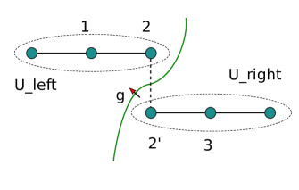
This method is particularly convenient for describing crystal defects. In the case of a single defect in supported along , where is a -dimensional branch cut (which, fixing , is a choice of gauge), the defect space can be covered with a single patch given by a thickening of , which intersects itself in along a neighborhood of . In other words, the degrees of freedom near the branch cut are doubled (see Figs 3, 5, and 11), coupled to either side of the branch cut, and then reglued by a projection map twisted by the crystal symmetry.
Appendix D Coupling smooth states to gauge fields
Here we prove the claims made in Section II.2 about the well-definedness of the construction to couple smooth states to gauge fields. We first consider the case of an internal symmetry . We adapt an argument due to Kitaev (Appendix F of Ref. Kitaev, 2006). We assume that our original ground state lives on a lattice with a spin of Hilbert space dimension at each site. However, we will define the space which our smooth states target to be the space of states with Hilbert space dimension per site. Of course, given a choice of isometric embedding , we could think of our original state as living in too. The resulting state depends on and we call it .
Recall that the symmetry is assumed to act on-site, with the action on each site described by a representation . For each , we also considered a path , such that and . Then, (at least locally) we can reformulate the prescription in Section II.2 for defining the smooth state as follows in terms of a spatially-dependent isometric embedding , according to . We then require that when passing over a patch boundary twisted by , goes through the continuous path obtained by acting with . But now we see that there will not be any obstructions to making this process well-defined due to non-contractible loops (or higher non-trivial homotopy groups) at intersections between patch boundaries, provided that we take sufficiently large. This is because in the limit the space of all isometric embeddings is contractible, i.e. all its homotopy groups are trivial.
A more rigorous (and succinct) way to think about the above construction is obtained by thinking about the classifying space . Indeed, since is a contractible space with a free action of , it follows that is a model for , and we find that there is a continuous map . A gauge field over is the same as a principal -bundle over , which can be represented by a a continuous map . Hence, composing these two maps gives a smooth state .
The “patch” version of the argument for a crystalline gauge field proceeds similarly to above and we will not write it out again. Let us simply note that a rigorous version of the construction can be formulated in terms of the homotopy quotient . Indeed, given a smooth state (where is the space of ground states with Hilbert space dimension per site), there is a map from defined by . This map is invariant under the diagional action of . Therefore, taking the limit , we find a map from . A crystalline gauge field on can be represented by a map from . By composing these two maps we obtain a smooth state .
Appendix E Lattice Crystalline Gauge Fields
The cellular description we give in this section is dual to the patch picture we gave in Section II.1, where elements labelled codimension 1 walls between volumes in the crystal. Here in order to compare with the usual definition of a lattice gauge field, we label edges with elements.
Recall for a discrete group a lattice gauge field has a very nice description where each edge gets a group label and any 2-face imposes a flatness constraint
| (17) |
where the multiplication is performed in the order the edges are encountered in a circular traversal of the boundary. This conservation law allows us to express these labels as a configuration of domain walls running about our manifold. The conservation law says that a and a fuse to a . The domain walls are codimension one so fusion can be non-commutative in this way.
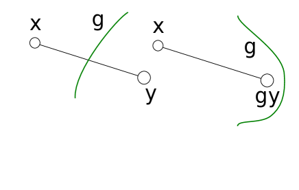
Let’s imagine drawing a configuration like this on where the elements act non-trivially on . Does this make sense? Let’s look at a particular edge, Fig 13. It looks like an edge from , but if we push the domain wall out of the way, we see the actual data there is an edge (actually path; see below) from to ! This means that while our underlying manifold has points labelled by points in , it is perhaps a different space ! To see what data is assigned to a face or higher facet, one performs a similar procedure, pushing all the domain walls off and collecting labels. The flatness condition on implies that this is always unambiguous. At a symmetry defect like the core of a disclination, the flatness condition is violated and it is impossible to unambiguously assign a face of to the core of the defect. When this happens, the underlying space may have different topology from ! In fact, we may end up with a space whose labels don’t even close up unto a map to ! In such a case, we end up with only a map , where is the -cover corresponding to the labels (equivalently the gauge bundle).
Note that if is contractible the extra information beyond the gauge field, the labels, contributes no non-trivial data up to homotopies of this map. Indeed this is basically another proof of the Crystalline Equivalence Principle.
Let us try to be more systematic about the construction. We start with a warm-up, just describing cellular maps in a lattice gauge theoryish way. A cellular map means the -skeleton of gets sent to the -skeleton of for every . This means every vertex gets a vertex , every edge gets a path , every plaquette gets a chain with , every volume gets a 3-chain with prescribed boundary and so on. This data describes a general partial covering (i.e. a map which gives a rigid crystalline gauge field with trivial transition functions).
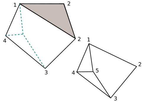
To account for maps which are not locally homeomorphisms, we need to include in this definition the degenerate facets of . For example, if we had the constant map , this definition only makes sense if there is a hidden edge , hidden faces , , and so on. All higher degenerate facets should be included as well.
This means that any map is homotopic to one given first by refinement of the lattice in and then by labelling vertices, edges, faces, … of the refinement with vertices, edges, faces, … (possibly degenerate ones) of . This should be intuitive, since the cell structure in is not really physical. It’s just a way to encode the topology of combinatorially.
Now let us consider maps with -twisted continuity conditions. As before we assign vertices of to vertices of . Before to an edge in we would assign a path connecting the labels and of the endpoints. For -fs, these paths can pass through domain walls, resulting in something we call a -path:
Around the boundary of a face , we get a -path by concatenating the -paths on each edge. Our conservation law
must be supplemented by the condition that the boundary -path forms a -loop:
If this is the case, then we can push all the ’s to the right, acting on the paths as we do to obtain an honest path . If the conservation law holds then this path is a loop in . This is just like pushing the domain walls off towards vertex . We ask that be assigned a chain with boundary equal to this loop. A picture of this is depicted in Fig 15.
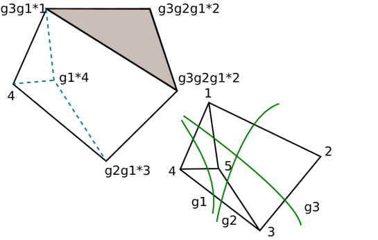
Now we discuss homotopies of this data (collapsible crystalline gauge transformations). Such a homotopy is itself a crystalline gauge field but on the prism with boundary conditions equal to and on each copy of .
As a first warm-up, let’s just consider ordinary gauge fields. See Fig 16. There is a cell complex of with one inner -cell for every cell of . These inner cells are the only ones where the boundary conditions do not fix the data. For an ordinary gauge field we must specify the labels on the inner edges. These correspond to vertices of , so the data is like an element of for each vertex of . The flatness condition on the inner faces determines how these must act on the edge variables.

A second warm-up, really getting going this time, is to consider homotopies of a map . This is the case with no symmetry, . This gets quite complicated but it is possible to divide homotopies into elementary pieces, where all the inner -cells but one are degenerate but one: , meaning the map does not change away from . The map identifies with a -chain and because all other inner cells in are degenerate, is divided into two -chains in the image of the boundaries: , where are -chains in . In fact these are the same -chains and is telling us how they move inside during the homotopy . A general gauge transformation of is essentially a combination of these two ingredients.
Just as the cellular description of gauge fields reflects a convenient cellular structure of , what we have described above amounts to a cellular structure on the homotopy quotient . One can see what we’ve written as a simultaneous construction of and a proof of
Theorem 6.
A crystalline gauge field is the same as a cellular map with the cell structure induced by the action of on a compatible cell structure of . Thus, gauge equivalence classes of crystalline gauge fields are the same as homotopy classes of maps .
There is a nice way to get a handle on the homotopy type of . Recall from, eg. Ref. Hatcher, 2002, that , the classifying space for ordinary -gauge fields and the special case of our construction when is a point, is itself constructed as an ordinary quotient , where is some (usually very large) contractible space on which acts freely. For discrete groups, can be constructed as a simplicial complex where vertices are group elements , edges are pairs, triangles are triples, and so on. The gluing maps use the multiplication. For example, an edge is glued to and to ; a triangle is glued to , ; and , and so on. This space has a action which acts on all the labels simultaneously. It’s also contractible. The quotient structure is the usual structure on . Likewise, we can invent a cell structure on the space so that the quotient structure is the one we’ve described on . This proves where acts diagonally. In fact, to preserve the homotopy type of , we just need any space which is homotopy equivalent to and on which acts freely. is an example, but if already acts freely on , then itself is an example and the homotopy quotient reduces to the ordinary quotient . In the other extreme, which is a purely internal symmetry, .
Appendix F Explicit constructions for bosonic SPTs
In Ref. Chen et al., 2013, a prescription was given to construct a ground-state wavefunction for an SPT phase protected by a finite internal symmetry group . As stated in the main text, we want to leverage this construction in a “bootstrap” procedure to construct a wavefunction for an SPT phase protected by a spatial symmetry, as outlined in Section III. For our current discussion, the important requirement is that we must be able to choose the wavefunction to be invariant under both an internal symmetry and a spatial symmetry . Ultimately, the symmetry protecting the crystalline SPT phase will be the diagonal subgroup . Recall that we take orientation-reversing elements of to also act anti-unitarily, in accordance with the CPT principle. (Thus, the orientation-reversing symmetries in are a composition of two anti-unitary operators, and so end up being unitary.)
Let us briefly review the construction of Ref. Chen et al., 2013. This construction starts from an element of the group cohomology group . This cohomology class is represented by a -cocycle in homogeneous form, which is a function satisfying
| (18) | |||
| (19) |
where denotes the action of on , i.e. anti-unitary elements of act by inversion.
To construct the wavefunction on some -dimensional spatial manifold, one first chooses a triangulation of the manifold. The spins will live on the vertices of this triangulation, and they will each carry a Hilbert space with basis , on which acts by left-multiplication: . Then one chooses a branching structure, which is a choice of direction on the edges of the triangulation, such that there are no directed cycles on any simplex. A branching structure allows us to define an ordering of the vertices on any -simplex. The wavefunction of Ref. Chen et al., 2013 is then defined as a superposition
| (20) |
where the sum is over all configurations of group elements for every vertex, and the product is over all -simplices. The phase factor associated to a -simplex is defined by
| (21) |
where are the group elements living on the vertices of the simplex (ordered according to the branching structure), is some fixed group element which is chosen to be the same for every -simplex (the resulting wavefunction turns out not to depend on on any closed manifold); and is the orientation of the -simplex (see Ref. Chen et al. (2013) for further details). It can be verified that the wavefunction so defined is indeed invariant under the action of .
Now it remains to show that can also be taken to be invariant under the action of a spatial symmetry . We take the action of on the Hilbert space of the spins to be inherited from its action on the space manifold; that is, it simply permutes the spins. (For orientation-reversing elements of , this is followed by complex conjugation, in accordance with our stipulation that orientation-reversing elements of should act anti-unitarily). This will evidently be the case provided that the locations of the vertices, the triangulation, and the branching structure are all invariant under the action of . (For orientation-revering elements, note that the effect of the complex conjugation is cancelled by the reversal of the orientation of the simplices). To achieve this, we can start from a -invariant cellulation of the spatial manifold (which can be obtained, for example, via the Wigner-Seitz construction), then take its barycentric subdivision, which gives a -invariant triangulation. Moreover, one can show that there is always a -invariant branching structure on this triangulation. The resulting triangulation and branching structure is illustrated in Figure 17 for the case and (the symmetry group of the simple square lattice).
Appendix G Cocycles
In this appendix, we delve a little deeper into what the equivariant cocycles mean. We will find they nicely formulate what it means for the cocycle (and hence the topological response) to be spatially-dependent. One can see this as another derivation of the equivariant cohomology classification. Importantly, we will learn how to integrate these cocycles.
G.1 Derivatives
We consider spacetime with its lattice it as a CW space. We want to define a “cocycle which depends on position”:
vHere is the dimension of . The local coefficients are there because we want our cocycle to be a pseudoscalar function, so that orientation reversing elements of conjugate the phase. This is important for getting the correct action of on and the correct classification in the case of time reversal symmetry and other orientation-reversing spacetime symmetries. In the rest of the section, we will take this coefficient system to be understood, just writing . Note that we cannot exchange the order of and in the above and get the right answers. In a sense, what we have is a group cochain valued in pseudoscalar functions on , ie. volume forms on .
We can define two differentials for such an object. The first measures a change in under a gauge transformation:
where in the first term we have used the action of on which we write as a right action. This reflects that when we write we are considering as a local coefficient system on induced by the action of on . To have a gauge invariant cocycle, we need
When this is true, we have a group cocycle valued in volume forms on .
There is another differential that measures whether the integral of this volume form defines a topological invariant of :
For , means that our cocycle is constant. However, it makes more sense to say that it is constant up to a gauge transformation. Thus, we should instead require
for some
It might not be possible to solve this equation. Indeed, we are asking that
be zero. If it is, then we can find and make a redefinition of our cocycle
To say that a homotopy of with its action can be compensated by a gauge transformation (and vice versa) we need to say . Inspecting what we have so far, we find
so we would like to find an with
The obstruction is
The pattern continues until the last obstruction
If we can solve all these descent equations, then we obtain a cocycle for both and , ie. both topological and gauge invariant:
Such a thing is called an equivariant cocycle and defines a class in ordinary equivariant cohomology .
Note we didn’t have to start with but could’ve instead started with a class in any of these groups:
with . Indeed, given any class , we can compute these differentials. If they all vanish, defines a class in equivariant cohomology . All classes in equivariant cohomology arise this way, but there may be new relations between classes and the group structure of may be some extension, with classes in combining into a class that comes from . The extension always goes in that direction and is always abelian.
The groups
have a very nice interpretation by decorating domain walls. It describes how codimension symmetry defects are decorated with forms.
G.2 Integrals
In this section we discuss how one computes the topological response Eq. 7 of Section IV.2
for and a cocycle described using the descent sequence of the previous section.
The integral is a sum over integrals for each -facet of . In order to evaluate the pullback on a -facet in , we decompose where and evaluate each and sum. The evaluation of works just like the cup product Hatcher (2002). This is simplest to describe in a simplical refinement of the cell structure on . All simplicies in are assumed to have ordered vertices. The first vertices with the labels on edges between them form a -simplex in on which we evaluate to obtain an element of . The last vertices with their edges and faces as above are
to which we can push all the ’s to the right to obtain a -chain in on which we evaluate that cochain, obtaining a number. The sum of these numbers is the value of on this -simplex of .
References
- Wen (1990) X.-G. Wen, Int. J. Mod. Phys. B 04, 239 (1990).
- Maciejko et al. (2010) J. Maciejko, X.-L. Qi, A. Karch, and S.-C. Zhang, Phys. Rev. Lett. 105, 246809 (2010), arXiv:1004.3628 .
- Essin and Hermele (2013) A. M. Essin and M. Hermele, Phys. Rev. B 87, 104406 (2013), arXiv:1212.0593 .
- Lu and Vishwanath (2013) Y.-M. Lu and A. Vishwanath, “Classification and Properties of Symmetry Enriched Topological Phases: A Chern-Simons approach with applications to Z2 spin liquids,” (2013), arXiv:1302.2634 .
- Mesaros and Ran (2013) A. Mesaros and Y. Ran, Phys. Rev. B 87, 155115 (2013), arXiv:1212.0835 .
- Hung and Wen (2013) L.-Y. Hung and X.-G. Wen, Phys. Rev. B 87, 165107 (2013), arXiv:1212.1827 .
- Barkeshli et al. (2014) M. Barkeshli, P. Bonderson, M. Cheng, and Z. Wang, “Symmetry, Defects, and Gauging of Topological Phases,” (2014), arXiv:1410.4540 .
- Cheng et al. (2015a) M. Cheng, M. Zaletel, M. Barkeshli, A. Vishwanath, and P. Bonderson, “Translational symmetry and microscopic constraints on symmetry-enriched topological phases: a view from the surface,” (2015a), arXiv:1511.02263 .
- Gu and Wen (2009) Z.-C. Gu and X.-G. Wen, Phys. Rev. B 80, 155131 (2009), arXiv:0903.1069 .
- Pollmann et al. (2010) F. Pollmann, A. M. Turner, E. Berg, and M. Oshikawa, Phys. Rev. B 81, 064439 (2010), arXiv:0910.1811 .
- Pollmann et al. (2012) F. Pollmann, E. Berg, A. M. Turner, and M. Oshikawa, Phys. Rev. B 85, 075125 (2012), arXiv:0909.4059 .
- Fidkowski and Kitaev (2010) L. Fidkowski and A. Kitaev, Phys. Rev. B 81, 134509 (2010), arXiv:0904.2197 .
- Chen et al. (2010) X. Chen, Z.-C. Gu, and X.-G. Wen, Phys. Rev. B 82, 155138 (2010), arXiv:1004.3835 .
- Chen et al. (2011a) X. Chen, Z.-C. Gu, and X.-G. Wen, Phys. Rev. B 83, 035107 (2011a), arXiv:1008.3745 .
- Schuch et al. (2011) N. Schuch, D. Pérez-García, and I. Cirac, Phys. Rev. B 84, 165139 (2011), arXiv:1010.3732 .
- Fidkowski and Kitaev (2011) L. Fidkowski and A. Kitaev, Phys. Rev. B 83, 075103 (2011), arXiv:1008.4138 .
- Chen et al. (2013) X. Chen, Z.-C. Gu, Z.-X. Liu, and X.-G. Wen, Phys. Rev. B 87, 155114 (2013), arXiv:1106.4772 .
- Chen et al. (2011b) X. Chen, Z.-X. Liu, and X.-G. Wen, Phys. Rev. B 84, 235141 (2011b), arXiv:1106.4752 .
- Vishwanath and Senthil (2013) A. Vishwanath and T. Senthil, Phys. Rev. X 3, 011016 (2013), arXiv:1209.3058 .
- Wang et al. (2014) C. Wang, A. C. Potter, and T. Senthil, Science 343, 629 (2014), arXiv:1306.3238 .
- Kapustin (2014) A. Kapustin, “Symmetry Protected Topological Phases, Anomalies, and Cobordisms: Beyond Group Cohomology,” (2014), arXiv:1403.1467 .
- Gu and Wen (2014) Z.-C. Gu and X.-G. Wen, Phys. Rev. B 90, 115141 (2014), arXiv:1201.2648 .
- Else and Nayak (2014) D. V. Else and C. Nayak, Phys. Rev. B 90, 235137 (2014), arXiv:1409.5436 .
- Burnell et al. (2014) F. J. Burnell, X. Chen, L. Fidkowski, and A. Vishwanath, Phys. Rev. B 90, 245122 (2014), arXiv:1302.7072 .
- Wang et al. (2015) J. C. Wang, Z.-C. Gu, and X.-G. Wen, Phys. Rev. Lett. 114, 031601 (2015), arXiv:1405.7689 .
- Cheng et al. (2015b) M. Cheng, Z. Bi, Y.-Z. You, and Z.-C. Gu, “Towards a Complete Classification of Symmetry-Protected Phases for Interacting Fermions in Two Dimensions,” (2015b), arXiv:1501.01313 .
- Kapustin et al. (2015) A. Kapustin, R. Thorngren, A. Turzillo, and Z. Wang, J. High Energy Phys. 2015, 1 (2015), arXiv:1406.7329 .
- Fu (2011) L. Fu, Phys. Rev. Lett. 106, 106802 (2011), arXiv:1010.1802 .
- Hsieh et al. (2012) T. H. Hsieh, H. Lin, J. Liu, W. Duan, A. Bansi, and L. Fu, Nat. Commun. 3, 982 (2012), arXiv:1202.1003 .
- Dziawa et al. (2012) P. Dziawa, B. J. Kowalski, K. Dybko, R. Buczko, A. Szczerbakow, M. Szot, E. Łusakowska, T. Balasubramanian, B. M. Wojek, M. H. Berntsen, O. Tjernberg, and T. Story, Nat. Mater. 11, 1023 (2012), arXiv:1206.1705 .
- Tanaka et al. (2012) Y. Tanaka, Z. Ren, T. Sato, K. Nakayama, S. Souma, T. Takahashi, K. Segawa, and Y. Ando, Nat. Phys. 8, 800 (2012), arXiv:arXiv:1304.0430 .
- Xu et al. (2012) S.-Y. Xu, C. Liu, N. Alidoust, M. Neupane, D. Qian, I. Belopolski, J. D. Denlinger, Y. J. Wang, H. Lin, L. a. Wray, G. Landolt, B. Slomski, J. H. Dil, a. Marcinkova, E. Morosan, Q. Gibson, R. Sankar, F. C. Chou, R. J. Cava, a. Bansil, and M. Z. Hasan, Nat. Commun. 3, 1192 (2012), arXiv:arXiv:1210.2917v1 .
- Zhang et al. (2013) F. Zhang, C. L. Kane, and E. J. Mele, Phys. Rev. Lett. 111, 056403 (2013), arXiv:1303.4144 .
- Fang et al. (2012) C. Fang, M. J. Gilbert, and B. A. Bernevig, Phys. Rev. B 86, 115112 (2012), arXiv:1207.5767 .
- Fang et al. (2013) C. Fang, M. J. Gilbert, and B. A. Bernevig, Phys. Rev. B 87, 035119 (2013), arXiv:1208.4603 .
- Chiu et al. (2013) C.-K. Chiu, H. Yao, and S. Ryu, Phys. Rev. B 88, 075142 (2013), arXiv:1303.1843 .
- Morimoto and Furusaki (2013) T. Morimoto and A. Furusaki, Phys. Rev. B 88, 125129 (2013), arXiv:1306.2505 .
- Slager et al. (2013) R.-J. Slager, A. Mesaros, V. Juričić, and J. Zaanen, Nat. Phys. 9, 98 (2013), arXiv:arXiv:1209.2610v2 .
- Shiozaki and Sato (2014) K. Shiozaki and M. Sato, Phys. Rev. B 90, 165114 (2014), arXiv:1403.3331 .
- Chiu et al. (2016) C.-K. Chiu, J. C. Y. Teo, A. P. Schnyder, and S. Ryu, Rev. Mod. Phys. 88, 035005 (2016), arXiv:1505.03535 .
- Isobe and Fu (2015) H. Isobe and L. Fu, Phys. Rev. B 92, 081304 (2015), arXiv:1502.06962 .
- Hsieh et al. (2014a) C.-T. Hsieh, T. Morimoto, and S. Ryu, Phys. Rev. B 90, 245111 (2014a), arXiv:1406.0307 .
- Qi and Fu (2015) Y. Qi and L. Fu, Phys. Rev. Lett. 115, 236801 (2015), arXiv:1505.06201 .
- Yoshida and Furusaki (2015) T. Yoshida and A. Furusaki, Phys. Rev. B 92, 085114 (2015), arXiv:arXiv:1505.06598v1 .
- Song and Schnyder (2016) X.-Y. Song and A. P. Schnyder, “Interaction effects on the classification of crystalline topological insulators and superconductors,” (2016), arXiv:1609.07469 .
- Wen (2002) X.-G. Wen, Phys. Rev. B 65, 165113 (2002), arXiv:cond-mat/0107071 .
- Hsieh et al. (2014b) C.-T. Hsieh, O. M. Sule, G. Y. Cho, S. Ryu, and R. G. Leigh, Phys. Rev. B 90, 165134 (2014b), arXiv:1403.6902 .
- Cho et al. (2015) G. Y. Cho, C.-T. Hsieh, T. Morimoto, and S. Ryu, Phys. Rev. B 91, 195142 (2015), arXiv:1501.07285 .
- Yoshida et al. (2015) T. Yoshida, T. Morimoto, and A. Furusaki, Phys. Rev. B 92, 245122 (2015), arXiv:1509.04395 .
- Lapa et al. (2016) M. F. Lapa, J. C. Y. Teo, and T. L. Hughes, Phys. Rev. B 93, 115131 (2016), arXiv:1409.1234 .
- You and Xu (2014) Y.-Z. You and C. Xu, Phys. Rev. B 90, 245120 (2014), arXiv:arXiv:1409.0168v1 .
- Hermele and Chen (2016) M. Hermele and X. Chen, Phys. Rev. X 6, 041006 (2016), arXiv:1508.00573 .
- Cheng et al. (2015c) M. Cheng, M. Zaletel, M. Barkeshli, A. Vishwanath, and P. Bonderson, “Translational symmetry and microscopic constraints on symmetry-enriched topological phases: a view from the surface,” (2015c), arXiv:1511.02263 .
- Jiang and Ran (2016) S. Jiang and Y. Ran, (2016), arXiv:1611.07652 .
- Song et al. (2016) H. Song, S.-J. Huang, L. Fu, and M. Hermele, “Topological phases protected by point group symmetry,” (2016), arXiv:1604.08151 .
- Chen et al. (2011c) X. Chen, Z.-C. Gu, and X.-G. Wen, Phys. Rev. B 84, 235128 (2011c), arXiv:1103.3323 .
- Dijkgraaf and Witten (1990) R. Dijkgraaf and E. Witten, Commun. Math. Phys. 129, 393 (1990).
- Levin and Gu (2012) M. Levin and Z.-C. Gu, Phys. Rev. B 86, 115109 (2012), arXiv:1202.3120 .
- Haah (2011) J. Haah, Phys. Rev. A 83, 042330 (2011), arXiv:1101.1962 .
- Yoshida (2013) B. Yoshida, Phys. Rev. B 88, 125122 (2013), arXiv:1302.6248 .
- Vijay et al. (2016) S. Vijay, J. Haah, and L. Fu, “Fracton Topological Order, Generalized Lattice Gauge Theory and Duality,” (2016), arXiv:1603.04442 .
- Williamson (2016) D. J. Williamson, Phys. Rev. B 94, 155128 (2016), arXiv:1603.05182 .
- Else and Nayak (2016) D. V. Else and C. Nayak, Phys. Rev. B 93, 201103 (2016), arXiv:1602.04804 .
- Hua (2017) “Building crystalline topological phases from lower-dimensional states,” (2017), 1705.09243 .
- Hunt et al. (2013) B. Hunt, J. D. Sanchez-Yamagishi, A. F. Young, M. Yankowitz, B. J. LeRoy, K. Watanabe, T. Taniguchi, P. Moon, M. Koshino, P. Jarillo-Herrero, and R. C. Ashoori, Science 340, 1427 (2013), arXiv:1303.6942 .
- Nakahara (2003) M. Nakahara, Geometry, Topology and Physics, Second Edition, Graduate student series in physics (Taylor & Francis, 2003).
- Drinfeld et al. (2009) V. Drinfeld, S. Gelaki, D. Nikshych, and V. Ostrik, ArXiv e-prints (2009), arXiv:0906.0620 [math.QA] .
- Kitaev (2006) A. Kitaev, Ann. Phys. (N. Y). 321, 2 (2006), arXiv:cond-mat/0506438 .
- Witten (1989) E. Witten, Comm. Math. Phys. 121, 351 (1989).
- Chen and Vishwanath (2015) X. Chen and A. Vishwanath, Phys. Rev. X 5, 041034 (2015), arXiv:1401.3736 .
- Etingof et al. (2009) P. Etingof, D. Nikshych, V. Ostrik, and w. a. a. b. Ehud Meir, ArXiv e-prints (2009), arXiv:0909.3140 [math.QA] .
- Baez and Dolan (1995) J. C. Baez and J. Dolan, J. Math. Phys. 36, 6073 (1995), arXiv:q-alg/9503002 .
- Kapustin and Thorngren (2013) A. Kapustin and R. Thorngren, “Higher symmetry and gapped phases of gauge theories,” (2013), arXiv:1309.4721 .
- Kapustin (2010) A. Kapustin, “Topological Field Theory, Higher Categories, and Their Applications,” (2010), arXiv:1004.2307 .
- Kapustin and Saulina (2011) A. Kapustin and N. Saulina, Nucl. Phys. B 845, 393 (2011), arXiv:1008.0654 .
- Fuchs et al. (2013) J. Fuchs, C. Schweigert, and A. Valentino, Communications in Mathematical Physics 321, 543 (2013).
- Henriques (2015) A. Henriques, (2015), arXiv:1503.06254 .
- Lurie (2009) J. Lurie, “On the Classification of Topological Field Theories,” (2009), arXiv:0905.0465 .
- Kapustin and Thorngren (2014a) A. Kapustin and R. Thorngren, (2014a), arXiv:1404.3230 [hep-th] .
- Freed and Hopkins (2016) D. S. Freed and M. J. Hopkins, “Reflection positivity and invertible topological phases,” (2016), arXiv:1604.06527 .
- Nikolaus et al. (2015) T. Nikolaus, U. Schreiber, and D. Stevenson, J. Homotopy Relat. Struct. 10, 749 (2015), arXiv:1207.0248 .
- Freed and Teleman (2012) D. S. Freed and C. Teleman, ArXiv e-prints (2012), arXiv:1212.1692 [hep-th] .
- Hiller (1986) H. Hiller, Am. Math. Mon. 93, 765 (1986).
- Hatcher (2002) A. Hatcher, Algebraic Topology (Cambridge University Press, 2002).
- Bi et al. (2015) Z. Bi, A. Rasmussen, K. Slagle, and C. Xu, Phys. Rev. B 91, 134404 (2015), arXiv:1309.0515 [cond-mat.str-el] .
- Khemani et al. (2016) V. Khemani, A. Lazarides, R. Moessner, and S. L. Sondhi, Phys. Rev. Lett. 116, 250401 (2016), arXiv:1508.03344 .
- von Keyserlingk and Sondhi (2016) C. W. von Keyserlingk and S. L. Sondhi, Phys. Rev. B 93, 245145 (2016), arXiv:1602.02157 .
- Potter et al. (2016) A. C. Potter, T. Morimoto, and A. Vishwanath, Phys. Rev. X 6, 041001 (2016), arXiv:1602.05194 .
- Roy and Harper (2016a) R. Roy and F. Harper, Phys. Rev. B 94, 125105 (2016a), arXiv:1602.08089 .
- Po et al. (2016) H. C. Po, L. Fidkowski, T. Morimoto, A. C. Potter, and A. Vishwanath, “Chiral Floquet Phases of Many-body Localized Bosons,” (2016), arXiv:1609.00006 .
- Potter and Morimoto (2016) A. C. Potter and T. Morimoto, (2016), arXiv:1610.03485 .
- Roy and Harper (2016b) R. Roy and F. Harper, “Floquet topological phases with symmetry in all dimensions,” (2016b), arXiv:1610.06899 .
- Shiozaki et al. (2016) K. Shiozaki, H. Shapourian, and S. Ryu, “Many-body topological invariants in fermionic symmetry protected topological phases,” (2016), arXiv:1609.05970 .
- Tarantino and Fidkowski (2016) N. Tarantino and L. Fidkowski, Phys. Rev. B 94, 115115 (2016), arXiv:1604.02145 .
- Gaiotto and Kapustin (2016) D. Gaiotto and A. Kapustin, Int. J. Mod. Phys. A 31, 1645044 (2016), arXiv:1505.05856 .
- Bhardwaj et al. (2016) L. Bhardwaj, D. Gaiotto, and A. Kapustin, “State sum constructions of spin-TFTs and string net constructions of fermionic phases of matter,” (2016), arXiv:1605.01640 .
- Ware et al. (2016) B. Ware, J. H. Son, M. Cheng, R. V. Mishmash, J. Alicea, and B. Bauer, Phys. Rev. B 94, 115127 (2016), arXiv:1605.06125 [cond-mat.str-el] .
- Bahri and Gilkey (1987) A. Bahri and P. Gilkey, Pac. J. Math. 128, 1 (1987).
- Litvin (2013) D. B. Litvin, Magnetic Group Tables (International Union of Crystallography, 2013).
- Thorngren (2015) R. Thorngren, J. High Energy Phys. 2015, 1 (2015), arXiv:1404.4385 .
- Aharony et al. (2013) O. Aharony, N. Seiberg, and Y. Tachikawa, JHEP 08, 115 (2013), arXiv:1305.0318 [hep-th] .
- Kapustin and Thorngren (2014b) A. Kapustin and R. Thorngren, Adv. Theor. Math. Phys. 18, 1233 (2014b), arXiv:1308.2926 [hep-th] .
- Kapustin and Seiberg (2014) A. Kapustin and N. Seiberg, JHEP 04, 001 (2014), arXiv:1401.0740 [hep-th] .
- Scaffidi et al. (2017) T. Scaffidi, D. E. Parker, and R. Vasseur, ArXiv e-prints (2017), arXiv:1705.01557 [cond-mat.str-el] .
- Abanov and Wiegmann (2000) A. G. Abanov and P. B. Wiegmann, Nucl. Phys. B570, 685 (2000), arXiv:hep-th/9911025 [hep-th] .
- Freed et al. (2017) D. S. Freed, Z. Komargodski, and N. Seiberg, (2017), arXiv:1707.05448 [cond-mat.str-el] .
- Haldane (1983) F. Haldane, Physics Letters A 93, 464 (1983).
- GAP (2016) “GAP – Groups, Algorithms, and Programming, Version 4.8.4,” http://www.gap-system.org (2016).