Streaming Principal Component Analysis From Incomplete Data

Abstract

Linear subspace models are pervasive in computational sciences and particularly used for large datasets which are often incomplete due to privacy issues or sampling constraints. Therefore, a critical problem is developing an efficient algorithm for detecting low-dimensional linear structure from incomplete data efficiently, in terms of both computational complexity and storage.

In this paper we propose a streaming subspace estimation algorithm called Subspace Navigation via Interpolation from Partial Entries ($\operatorname{SNIPE}$) that efficiently processes blocks of incomplete data to estimate the underlying subspace model. In every iteration, $\operatorname{SNIPE}$ finds the subspace that best fits the new data block but remains close to the previous estimate. We show that $\operatorname{SNIPE}$ is a streaming solver for the underlying nonconvex matrix completion problem, that it converges globally to a stationary point of this program regardless of initialization, and that the convergence is locally linear with high probability. We also find that $\operatorname{SNIPE}$ shows state-of-the-art performance in our numerical simulations.

Keywords— Principal component analysis, Subspace identification, Matrix completion, Streaming algorithms, Nonconvex optimization, Global convergence.

1 Introduction

Linear models are the backbone of computational science, and Principal Component Analysis (PCA) in particular is an indispensable tool for detecting linear structure in collected data [1, 2, 3, 4]. Principal components of a dataset are used, for example, to perform linear dimensionality reduction, which is in turn at the heart of classification, regression and other learning tasks that often suffer from the “curse of dimensionality”, where having a small number of training samples in relation to the number of features typically leads to overfitting [5].

In this work, we are particularly interested in applying PCA to data that is presented sequentially to a user, with limited processing time available for each item. Moreover, due to hardware limitations, we assume the user can only store small amounts of data. Finally, we also consider the possibility that the incoming data is incomplete, either due to physical sampling constraints, or deliberately subsampled to facilitate faster processing times or to address privacy concerns.

As one example, consider monitoring network traffic over time, where acquiring complete network measurements at fine time-scales is impractical and subsampling is necessary [6, 7]. As another example, suppose we have a network of cheap, battery-powered sensors that must relay summary statistics of their measurements, say their principal components, to a central node on a daily basis. Each sensor cannot store or process all its daily measurements locally, nor does it have the power to relay all the raw data to the central node. Moreover, many measurements are not reliable and can be treated as missing. It is in this and similar contexts that we hope to develop a streaming algorithm for PCA from incomplete data.

More formally, we consider the following problem: Let $\mathcal{S}$ be an $r$-dimensional subspace with orthonormal basis $S\in\mathbb{R}^{n\times r}$. For an integer $T$, let the coefficient vectors $\{q_{t}\}_{t=1}^{T}\subset\mathbb{R}^{r}$ be independent copies of a random vector $q\in\mathbb{R}^{r}$ with bounded expectation, namely $\mathbb{E}\|q\|_{2}<\infty$. Consider the sequence of vectors $\{Sq_{t}\}_{t=1}^{T}\subset\mathcal{S}$ and set $s_{t}:=Sq_{t}$ for short. At each time $t\in[1:T]:=\{1,2,\cdots,T\}$, we observe each entry of $s_{t}$ independently with a probability of $p$ and collect the observed entries in $y_{t}\in\mathbb{R}^{n}$. Formally, we let $\omega_{t}\subseteq[1:n]$ be the random index set over which $s_{t}$ is observed and write this measurement process as $y_{t}=P_{\omega_{t}}\cdot s_{t}$, where $P_{\omega_{t}}\in\mathbb{R}^{n\times n}$ is the projection onto the coordinate set $\omega_{t}$, namely it equals one on its diagonal entries corresponding to the index set $\omega_{t}$ and is zero elsewhere.

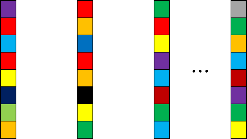
(a)

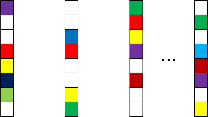
(b)

Figure 1: The sequence of generic vectors $\{s_{t}\}_{t=1}^{T}$ drawn from an unknown $r$-dimensional subspace $\mathcal{S}$ in panel (a) is only partially observed on random index sets $\{\omega_{t}\}_{t=1}^{T}$. That is, we only have access to incomplete data vectors $\{y_{t}\}_{t=1}^{T}$ in panel (b), where the white entries are missing. Our objective is to estimate the subspace $\mathcal{S}$ from the incomplete data vectors, when limited storage and processing resources are available. See Section 1 for the detailed setup.

Our objective in this paper is to design a streaming algorithm to identify the subspace $\mathcal{S}$ from the incomplete data $\{y_{t}\}_{t=1}^{T}$ supported on the index sets $\{\omega_{t}\}_{t=1}^{T}$. Put differently, our objective is to design a streaming algorithm to compute leading $r$ principal components of the full (but hidden) data matrix $[s_{1}\,s_{2}\cdots s_{T}]$ from the incomplete observations $[y_{1}\,y_{2}\,\cdots y_{T}]$, see Figure 1. By the Eckart-Young-Mirsky Theorem, this task is equivalent to computing leading $r$ left singular vectors of the full data matrix from its partial observations [8, 9].

Assuming that $r=\mbox{dim}(\mathcal{S})$ is known a priori (or estimated from data by other means), we present the $\operatorname{SNIPE}$ algorithm for this task in Section 2. $\operatorname{SNIPE}$ is designed based on the principle of least-change and, in every iteration, finds the subspace that best fits the new data block but remains close to the previous estimate. $\operatorname{SNIPE}$ requires $O(n)$ bits of memory and performs $O(n)$ flops in every iteration, which is optimal in its dependence on the ambient dimension $n$. As discussed in Section 3, $\operatorname{SNIPE}$ has a natural interpretation as a streaming algorithm for low-rank matrix completion [10].

Section 4 discusses the global and local convergence of $\operatorname{SNIPE}$. In particular, the local convergence rate is linear near the true subspace, namely the estimation error of $\operatorname{SNIPE}$ reduces by a factor of $1-cp$ in every iteration, for a certain factor $c$ and with high probability. This local convergence guarantee for $\operatorname{SNIPE}$ is a key technical contribution of this paper which is absent in its close competitors, see Section 5.

Even though we limit ourselves to the “noise-free” case of $y_{t}=P_{\omega_{t}}s_{t}$ in this paper, $\operatorname{SNIPE}$ can also be applied (after minimal changes) when $y_{t}=P_{\omega_{t}}(s_{t}+n_{t})$, where we might think of $n_{t}\in\mathbb{R}^{n}$ as measurement noise from a signal processing viewpoint. Alternatively from a statistical viewpoint, $n_{t}$ represents the tail of the covariance matrix of the generative model, from which $\{s_{t}\}_{t}$ are drawn. Moreover, $\operatorname{SNIPE}$ can be easily adapted to the dynamic case where the underlying subspace $\mathcal{S}=\mathcal{S}(t)$ changes over time. We leave the convergence analysis of $\operatorname{SNIPE}$ under a noisy time-variant model to a future work. Similarly, entries of incoming vectors are observed uniformly at random in our theoretical analysis but $\operatorname{SNIPE}$ also applies to any incomplete data.

A review of prior art is presented in Section 5, and the performance of $\operatorname{SNIPE}$ and rival algorithms are examined numerically in Section 6, where we find that $\operatorname{SNIPE}$ shows the state-of-the-art performance. Technical proofs appear in Section 7 and in the appendices, with Appendix A (Toolbox) collecting some of the frequently-used mathematical tools. Finally, Appendix L offers an alternative initialization for $\operatorname{SNIPE}$.

2 SNIPE

In this section, we present Subspace Navigation via Interpolation from Partial Entries (SNIPE), a streaming algorithm for subspace identification from incomplete data, received sequentially.

Let us first introduce some additional notation. Recall that we denote the incoming sequence of incomplete vectors by $\{y_{t}\}_{t=1}^{T}\subset\mathbb{R}^{n}$, which are supported on index sets $\{\omega_{t}\}_{t=1}^{T}\subseteq[1:n]$. For a block size $b\geq r$, we concatenate every $b$ consecutive vectors into a data block, thereby partitioning the incoming data into $K=T/b$ non-overlapping blocks $\{Y_{k}\}_{k=1}^{K}$, where $Y_{k}\in\mathbb{R}^{n\times b}$ for every $k$. We assume for convenience that $K$ is an integer. We also often take $b=O(r)$ to maximize the efficiency of SNIPE, as discussed below.

At a high level, $\operatorname{SNIPE}$ processes the first incomplete block $Y_{1}$ to produce an estimate $\widehat{\mathcal{S}}_{1}$ of the true subspace $\mathcal{S}$. This estimate is then iteratively updated after receiving each of the new incomplete blocks $\{Y_{k}\}_{k=2}^{K}$, thereby producing a sequence of estimates $\{\widehat{\mathcal{S}}_{k}\}_{k=2}^{K}$ , see Figure 2. Every $\widehat{\mathcal{S}}_{k}$ is an $r$-dimensional subspace of $\mathbb{R}^{n}$ with orthonormal basis $\widehat{S}_{k}\in\mathbb{R}^{n\times r}$; the particular choice of orthonormal basis is inconsequential throughout the paper.

Figure 2: $\operatorname{SNIPE}$ concatenates every $b$ incoming vectors into a block and iteratively updates its estimate of the true subspace $\mathcal{S}$ after receiving each new block. That is, $\operatorname{SNIPE}$ updates its estimate of $\mathcal{S}$, from $\widehat{\mathcal{S}}_{k-1}$ to $\widehat{\mathcal{S}}_{k}$, after receiving the incomplete data block $Y_{k}\in\mathbb{R}^{n\times b}$, see Section 2 for the details.

More concretely, $\operatorname{SNIPE}$ sets $\widehat{\mathcal{S}}_{1}$ to be the span of leading $r$ left singular vectors of $Y_{1}$, namely the left singular vectors corresponding to largest $r$ singular values of $Y_{1}$, with ties broken arbitrarily. Then, at iteration $k\in[2:K]$ and given the previous estimate $\widehat{\mathcal{S}}_{k-1}=\mbox{span}(\widehat{S}_{k-1})$, $\operatorname{SNIPE}$ processes the columns of the $k$th incomplete block $Y_{k}$ one by one and forms the matrix

$$R_{k}=\left[\begin{array}[]{ccc}\cdots&y_{t}+P_{\omega_{t}^{C}}\widehat{S}_{k-1}\left(\widehat{S}_{k-1}^{*}P_{\omega_{t}}\widehat{S}_{k-1}+\lambda I_{r}\right)^{\dagger}\widehat{S}_{k-1}^{*}y_{t}&\cdots\end{array}\right]\in\mathbb{R}^{n\times b},\qquad t\in[(k-1)b+1:kb],$$ (1)

where $\dagger$ denotes the pseudo-inverse and $\lambda\geq 0$ is a parameter. Above, $P_{\omega_{t}^{C}}=I_{n}-P_{\omega_{t}}\in\mathbb{R}^{n\times n}$ projects a vector onto the complement of the index set $\omega_{t}$. The motivation for the particular choice of $R_{k}$ above will become clear in Section 3. $\operatorname{SNIPE}$ then updates its estimate by setting $\widehat{\mathcal{S}}_{k}$ to be the span of leading $r$ left singular vectors of $R_{k}$. Algorithm 1 summarizes these steps. Note that Algorithm 1 rejects ill-conditioned updates in Step 3 for the convenience of analysis and that similar reject options have precedence in the literature [11]. We however found implementing this reject option to be unnecessary in numerical simulations.

Remark 1.

[Computational complexity of SNIPE] We measure the algorithmic complexity of $\operatorname{SNIPE}$ by calculating the average number of floating-point operations (flops) performed on an incoming vector. Every iteration of $\operatorname{SNIPE}$ involves finding leading $r$ left singular vectors of an $n\times b$ matrix. Assuming that $b=O(r)$, this could be done with $O(nr^{2})$ flops. At the $k$th iteration with $k\geq 2$, $\operatorname{SNIPE}$ also requires finding the pseudo-inverse of $P_{\omega_{j}}\widehat{S}_{k-1}\in\mathbb{R}^{n\times r}$ for each incoming vector which costs $O(nr^{2})$ flops. Therefore the overall computational complexity of $\operatorname{SNIPE}$ is $O(nr^{2})$ flops per vector. As further discussed in Section 5, this matches the complexity of other algorithms for streaming PCA even though here the received data is highly incomplete. ∎

Remark 2.

[Storage requirements of SNIPE] We measure the storage required by $\operatorname{SNIPE}$ by calculating the number of memory elements stored by $\operatorname{SNIPE}$ at any given instant. At the $k$th iteration, $\operatorname{SNIPE}$ must store the current estimate $\widehat{S}_{k-1}\in\mathbb{R}^{n\times r}$ (if available) and the new incomplete block $Y_{k}\in\mathbb{R}^{n\times b}$. Assuming that $b=O(r)$, this translates into $O(nr)+O(pnr)=O(nr)$ memory elements. $\operatorname{SNIPE}$ therefore requires $O(nr)$ bits of storage, which is optimal up to a constant factor. ∎

Algorithm 1 $\operatorname{SNIPE}$ for streaming PCA from incomplete data

Input:

• Dimension $r$,

• Received data $\{y_{t}\}_{t=1}^{T}\subset\mathbb{R}^{n}$ supported on index sets $\{\omega_{t}\}_{t=1}^{T}\subseteq[1:n]$, presented sequentially in $K=T/b$ blocks of size $b\geq r$,

• Tuning parameter $\lambda\geq 0$,

• Reject thresholds $\sigma_{\min},\tau\geq 0$.

Output:

• $r$-dimensional subspace $\widehat{\mathcal{S}}_{K}$.

Body:

• Form $Y_{1}\in\mathbb{R}^{n\times b}$ by concatenating the first $b$ received vectors $\{y_{t}\}_{t=1}^{b}$. Let $\widehat{\mathcal{S}}_{1}$, with orthonormal basis $\widehat{S}_{1}\in\mathbb{R}^{n\times r}$, be the span of leading $r$ left singular vectors of $Y_{1}$, namely those corresponding to $r$ largest singular values. Ties are broken arbitrarily.

• For $k\in[2:K]$, repeat:

  1. Set $R_{k}\leftarrow\{\}$.

  2. For $t\in[(k-1)b+1:kb]$, repeat

     • Set

       $$R_{k}\leftarrow\left[\begin{array}[]{cc}R_{k}&y_{t}+P_{\omega_{t}^{C}}\widehat{S}_{k-1}\left(\widehat{S}_{k-1}^{*}P_{\omega_{t}}\widehat{S}_{k-1}+\lambda I_{r}\right)^{\dagger}\widehat{S}_{k-1}^{*}y_{t}\end{array}\right],$$

       where $P_{\omega_{t}}\in\mathbb{R}^{n\times n}$ equals one on its diagonal entries corresponding to the index set $\omega_{t}$, and is zero elsewhere. Likewise, $P_{\omega_{t}^{C}}$ projects a vector onto the complement of the index set $\omega_{t}$.

  3. If $\sigma_{r}(R_{k})<\sigma_{\min}$ or $\sigma_{r}(R_{k})\leq(1+\tau)\cdot\sigma_{r+1}(R_{k})$, then set $\widehat{\mathcal{S}}_{k}\leftarrow\widehat{\mathcal{S}}_{k-1}$. Otherwise, let $\widehat{\mathcal{S}}_{k}$, with orthonormal basis $\widehat{S}_{k}\in\mathbb{R}^{n\times r}$, be the span of leading $r$ left singular vectors of $R_{k}$. Ties are broken arbitrarily. Here, $\sigma_{i}(R_{k})$ is the $i$th largest singular value of $R_{k}$.

• Return $\widehat{\mathcal{S}}_{K}$.

3 Interpretation of SNIPE

$\operatorname{SNIPE}$ has a natural interpretation as a streaming algorithm for low-rank matrix completion, which we now discuss. First let us enrich our notation. Recall the incomplete data blocks $\{Y_{k}\}_{k=1}^{K}\subset\mathbb{R}^{n\times b}$ and let the random index set $\Omega_{k}\subseteq[1:n]\times[1:b]$ be the support of $Y_{k}$ for every $k$. We write that $Y_{k}=P_{\Omega_{k}}(S_{k})$ for every $k$, where the complete (but hidden) data block $S_{k}\in\mathbb{R}^{n\times b}$ is formed by concatenating $\{s_{t}\}_{t=(k-1)b+1}^{kb}$. Here, $P_{\Omega_{k}}(S_{k})$ retains only the entries of $S_{k}$ on the index set $\Omega_{k}$, setting the rest to zero. By design, $s_{t}=Sq_{t}$ for every $t$ and we may therefore write that $S_{k}=S\cdot Q_{k}$ for the coefficient matrix $Q_{k}\in\mathbb{R}^{r\times b}$ formed by concatenating $\{q_{t}\}_{t=(k-1)b+1}^{kb}$. To summarize, $\{S_{k}\}_{k=1}^{K}$ is formed by partitioning $\{s_{t}\}_{t=1}^{T}$ into $K$ blocks. Likewise, $\{Q_{k},Y_{k},\Omega_{k}\}_{k=1}^{K}$ are formed by partitioning $\{q_{t},y_{t},\omega_{t}\}_{t=1}^{T}$, respectively.

With this introduction, let us form $Y\in\mathbb{R}^{n\times T}$ by concatenating the incomplete blocks $\{Y_{k}\}_{k=1}^{K}\subset\mathbb{R}^{n\times b}$, supported on the index sets $\Omega\subseteq[1:n]\times[1:T]$. To find the true subspace $\mathcal{S}$, one might consider solving

$$\begin{cases}\underset{X,\mathcal{U}}{\min}\,\,\,\left\|P_{\mathcal{U}^{\perp}}X\right\|_{F}^{2}+\lambda\|P_{\Omega^{C}}(X)\|_{F}^{2}\\ P_{\Omega}\left(X\right)=Y,\end{cases}$$ (2)

where the minimization is over a matrix $X\in\mathbb{R}^{n\times T}$ and $r$-dimensional subspace $\mathcal{U}\subset\mathbb{R}^{n}$. Above, $P_{\mathcal{U}^{\perp}}\in\mathbb{R}^{n\times n}$ is the orthogonal projection onto the orthogonal complement of subspace $\mathcal{U}$ and $P_{\Omega}(X)$ retains only the entries of $X$ on the index set $\Omega$, setting the rest to zero. Note that Program (2) encourages its solution(s) to be low-rank while matching the observations $Y$ on the index set $\Omega$. The term $\lambda\|P_{\Omega^{C}}(X)\|_{F}^{2}$ for $\lambda\geq 0$ is the Tikhonov regularizer that controls the energy of solution(s) on the complement of index set $\Omega$.

With complete data, namely when $\Omega=[1:n]\times[1:T]$, Program (2) reduces to PCA, as it returns $X=Y$ and searches for an $r$-dimensional subspace that captures most of the energy of $Y$. That is, Program (2) reduces to $\min_{\mathcal{U}}\|P_{\mathcal{U}^{\perp}}Y\|_{F}^{2}$ when $\Omega=[1:n]\times[1:T]$, solution of which is the span of leading $r$ left singular vectors of $Y$ in light of the Eckart-Young-Mirsky Theorem [8, 9]. In this sense then, Program (2) performs PCA from incomplete data. Note crucially that Program (2) is a nonconvex problem because the Grassmannian $\mathbb{G}(n,r)$, the set of all $r$-dimensional subspaces in $\mathbb{R}^{n}$, is a nonconvex set. However, given a fixed subspace $\mathcal{U}\in\mathbb{G}(n,r)$, Program (2) reduces to the simple least-squares program

$$\begin{cases}\underset{X}{\min}\,\,\,\left\|P_{\mathcal{U}^{\perp}}X\right\|_{F}^{2}+\lambda\|P_{\Omega^{C}}(X)\|_{F}^{2}\\ P_{\Omega}\left(X\right)=Y,\end{cases}$$ (3)

where the minimization is over $X\in\mathbb{R}^{n\times T}$. If in addition $\lambda$ is positive, then Program (3) is strongly convex and has a unique minimizer. Given a fixed feasible $X\in\mathbb{R}^{n\times T}$, Program (2) has the same minimizers as

$$\underset{\mathcal{U}\in\mathbb{G}(n,r)}{\min}\|P_{\mathcal{U}^{\perp}}X\|_{F}^{2}.$$ (4)

That is, for a fixed feasible $X$, Program (2) simply performs PCA on $X$. We might also view Program (2) from a matrix completion perspective. More specifically, let

$$\rho_{r}^{2}(X)=\sum_{i\geq r+1}\sigma_{i}^{2}(X),$$ (5)

be the residual of $X$, namely the energy of its trailing singular values $\sigma_{r+1}(X)\geq\sigma_{r+2}(X)\geq\cdots$. Like the popular nuclear norm $\|X\|_{*}=\sum_{i\geq 1}\sigma_{i}(X)$ in [10], the residual $\rho_{r}(X)$ gauges the rank of $X$. In particular, $\rho_{r}(X)=0$ if and only if $\mbox{rank}(X)\leq r$. Unlike the nuclear norm, however, the residual is still a nonconvex function of $X$. We now rewrite Program (2) as

$$\begin{cases}\underset{X,\mathcal{U}}{\min}\,\,\,\left\|P_{\mathcal{U}^{\perp}}X\right\|_{F}^{2}+\lambda\|P_{\Omega^{C}}(X)\|_{F}^{2}\\ P_{\Omega}\left(X\right)=Y\end{cases} =\begin{cases}\underset{X}{\min}\,\,\,\underset{\mathcal{U}\in\mathbb{G}(n,r)}{\min}\,\,\,\left\|P_{\mathcal{U}^{\perp}}X\right\|_{F}^{2}+\lambda\|P_{\Omega^{C}}(X)\|_{F}^{2}\\ P_{\Omega}\left(X\right)=Y\end{cases}$$

$$=\begin{cases}\underset{X}{\min}\,\,\,\rho_{r}^{2}(X)+\lambda\|P_{\Omega^{C}}(X)\|_{F}^{2}\\ P_{\Omega}\left(X\right)=Y.\end{cases}$$ (6)

That is, if we ignore the regularization term $\lambda\|P_{\Omega^{C}}(X)\|_{F}^{2}$, Program (2) searches for a matrix with the least residual, as a proxy for least rank, that matches the observations $Y$. In this sense then, Program (2) is a “relaxation” of the low-rank matrix completion problem. Several other formulations for the matrix completion problem are reviewed in [10, 12, 13]. We can also rewrite Program (2) in terms of its data blocks by considering the equivalent program

$$\begin{cases}\min\,\,\,\sum_{k=1}^{K}\|P_{\mathcal{U}}^{\perp}X_{k}\|_{F}^{2}+\lambda\|P_{\Omega_{k}^{C}}(X_{k})\|_{F}^{2}\\ P_{\Omega_{k}}\left(X_{k}\right)=Y_{k}\qquad k\in[1:K],\end{cases}$$ (7)

where the minimization is over matrices $\{X_{k}\}_{k=1}^{K}\subset\mathbb{R}^{n\times b}$ and subspace $\mathcal{U}\in\mathbb{G}(n,r)$. Let us additionally introduce a number of auxiliary variables into Program (7) by considering the equivalent program

$$\begin{cases}\min\,\,\,\sum_{k=1}^{K}\|P_{\mathcal{U}_{k}}^{\perp}X_{k}\|_{F}^{2}+\lambda\|P_{\Omega_{k}^{C}}(X_{k})\|_{F}^{2}\\ P_{\Omega_{k}}\left(X_{k}\right)=Y_{k}\qquad k\in[1:K]\\ \mathcal{U}_{1}=\mathcal{U}_{2}=\cdots=\mathcal{U}_{K},\end{cases}$$ (8)

where the minimization is over matrices $\{X_{k}\}_{k=1}^{K}\subset\mathbb{R}^{n\times b}$ and subspaces $\{\mathcal{U}_{k}\}_{k=1}^{K}\subset\mathbb{G}(n,r)$. Indeed, Programs (2,7,8) are all equivalent and all nonconvex. Now consider the following approximate solver for Program (8) that alternatively solves for matrices and subspaces:

• Setting $X_{1}=Y_{1}$ in Program (8), we minimize $\|P_{\mathcal{U}_{1}}^{\perp}Y_{1}\|_{F}^{2}$ over $\mathcal{U}_{1}\in\mathbb{G}(n,r)$ and, by the Eckart-Young-Mirsky Theorem, find a minimizer to be the span of leading $r$ left singular vectors of $Y_{1}$, which coincides with $\widehat{\mathcal{S}}_{1}$ in $\operatorname{SNIPE}$.

• For $k\in[2:K]$, repeat:

  • Setting $\mathcal{U}_{k}=\widehat{\mathcal{S}}_{k-1}$ in Program (8), we solve

    $$\begin{cases}\min_{X_{k}}\,\,\,\|P_{\widehat{\mathcal{S}}_{k-1}^{\perp}}X_{k}\|_{F}^{2}+\lambda\|P_{\Omega_{k}^{C}}(X_{k})\|_{F}^{2}\\ P_{\Omega_{k}}\left(X_{k}\right)=Y_{k},\end{cases}$$ (9)

    over matrix $X_{k}\in\mathbb{R}^{n\times b}$. We verify in Appendix B that the minimizer of Program (9) coincides with $R_{k}$ in $\operatorname{SNIPE}$, see (1).

  • If $\sigma_{r}(R_{k})<\sigma_{\min}$ or $\sigma_{r}(R_{k})\leq(1+\tau)\sigma_{r+1}(R_{k})$, then no update is made, namely we set $\widehat{\mathcal{S}}_{k}=\widehat{\mathcal{S}}_{k-1}$. Otherwise, setting $X_{k}=R_{k}$ in Program (8), we solve $\min\|P_{\mathcal{U}_{k}}^{\perp}R_{k}\|_{F}^{2}$ over $\mathcal{U}_{k}\in\mathbb{G}(n,r)$ to find $\widehat{\mathcal{S}}_{k}$. That is, by the Eckart-Young-Mirsky Theorem again, $\widehat{\mathcal{S}}_{k}$ is the span of leading $r$ left singular vectors of $R_{k}$. The output of this step matches $\widehat{\mathcal{S}}_{k}$ produced in $\operatorname{SNIPE}$.

To summarize, following the above procedure produces $\{R_{k}\}_{k=1}^{K}$ and $\{\widehat{\mathcal{S}}_{k}\}_{k=1}^{K}$ in $\operatorname{SNIPE}$. In other words, we might think of $\operatorname{SNIPE}$ as an approximate solver for Program (2), namely $\operatorname{SNIPE}$ is a streaming algorithm for low-rank matrix completion. In fact, the output of $\operatorname{SNIPE}$ always converges to a stationary point of Program (2) in the sense described in Section 4.

Another insight about the choice of $R_{k}$ in (1) is as follows. Let us set $\lambda=0$ for simplicity. At the beginning of the $k$th iteration of $\operatorname{SNIPE}$ with $k\geq 2$, the available estimate of the true subspace is $\widehat{\mathcal{S}}_{k-1}$ with orthonormal basis $\widehat{S}_{k-1}$. Given a new incomplete vector $y\in\mathbb{R}^{n}$, supported on the index set $\omega\subseteq[1:n]$, $z=\widehat{S}_{k-1}(P_{\omega}\widehat{S}_{k-1})^{\dagger}y$ best approximates $y$ in $\widehat{\mathcal{S}}_{k-1}$ in $\ell_{2}$ sense. In order to agree with the measurements, we minimally adjust this to $y+P_{\omega^{C}}z$, where $P_{\omega^{C}}$ projects onto the complement of index set $\omega$. This indeed matches the expression for the columns of $R_{k}$ in $\operatorname{SNIPE}$. We note that this type of least-change strategy has been successfully used in the development of quasi-Newton methods for optimization [14, Chapter 6].

4 Performance of SNIPE

To measure the performance of $\operatorname{SNIPE}$—whose output is a subspace—we naturally use principal angles as an error metric. More specifically, recall that $\mathcal{S}$ and $\widehat{\mathcal{S}}_{K}$ denote the true subspace and the output of $\operatorname{SNIPE}$, respectively. Then the $i$th largest singular value of $P_{\mathcal{S}^{\perp}}P_{\widehat{\mathcal{S}}_{K}}$ equals $\sin(\theta_{i}(\mathcal{S},\widehat{\mathcal{S}}_{K}))$, where

$$\theta_{1}(\mathcal{S},\widehat{\mathcal{S}}_{K})\geq\theta_{2}(\mathcal{S},\widehat{\mathcal{S}}_{K})\geq\cdots\geq\theta_{r}(\mathcal{S},\widehat{\mathcal{S}}_{K})$$

denote the principal angles between the two $r$-dimensional subspaces $\mathcal{S},\widehat{\mathcal{S}}_{K}$ [15]. The estimation error of $\operatorname{SNIPE}$ is then

$$d_{\mathbb{G}}(\mathcal{S},\widehat{\mathcal{S}}_{K}):=\sqrt{\frac{1}{r}\sum_{i=1}^{r}\sin^{2}\left(\theta_{i}(\mathcal{S},\widehat{\mathcal{S}}_{K})\right)}=\frac{\|P_{\mathcal{S}^{\perp}}P_{\widehat{\mathcal{S}}_{K}}\|_{F}}{\sqrt{r}},$$ (10)

which also naturally induces a metric topology on the Grassmannian $\mathbb{G}(n,r)$. Note also that we will always reserve calligraphic letters for subspaces and capital letters for their orthonormal bases, for example subspace $\mathcal{S}$ and its orthonormal basis $S$.

Our first result loosely speaking states that a subsequence of $\operatorname{SNIPE}$ converges to a stationary point of the nonconvex Program (2) as $T$ goes to infinity, see Section 7.1 for the proof.

Theorem 1.

[Global convergence] Consider an $r$-dimensional subspace $\mathcal{S}$ with orthonormal basis $S\in\mathbb{R}^{n\times r}$. For an integer $T$, let the coefficient vectors $\{q_{t}\}_{t=1}^{T}\subset\mathbb{R}^{r}$ be independent copies of a random vector $q\in\mathbb{R}^{r}$ with bounded expectation, namely $\mathbb{E}\|q\|_{2}<\infty$. For every $t\in[1:T]$, we observe each coordinate of $s_{t}=Sq_{t}\in\mathcal{S}$ independently with a probability of $p$ and collect the observations in $y_{t}\in\mathbb{R}^{n}$, supported on a random index set $\omega_{t}\subseteq[1:n]$. Fix positive $\lambda$, block size $b\geq r$, positive reject thresholds $\sigma_{\min},\tau$, and consider the output sequence of $\operatorname{SNIPE}$ in Algorithm 1, namely $\{(R_{k},\widehat{\mathcal{S}}_{k})\}_{k}$. Also by partitioning $\{q_{t},s_{t},y_{t},\omega_{t}\}_{t}$, form the coefficient blocks $\{Q_{k}\}_{k}\subset\mathbb{R}^{r\times b}$, data blocks $\{S_{k}\}_{k}\subset\mathbb{R}^{n\times b}$, and incomplete data blocks $\{Y_{k}\}_{k}\subset\mathbb{R}^{n\times b}$ supported on index sets $\{\Omega_{k}\}_{k}\subseteq[1:n]\times[1:b]$, as described in Section 3.

For every integer $l$, there exists an integer $k_{l}$, for which the following asymptotic statement is almost surely true as $T\rightarrow\infty$. Consider the restriction of Program (2) to iteration $k_{l}$, namely

$$\begin{cases}\min_{X,\mathcal{U}}\,\,\,\|P_{\mathcal{U}^{\perp}}X\|_{F}^{2}+\lambda\|P_{\Omega_{k_{l}}^{C}}(X)\|_{F}^{2}\\ P_{\Omega_{k_{l}}}(X)=Y_{k_{l}},\end{cases}$$ (11)

where the minimization is over matrix $X\in\mathbb{R}^{n\times b}$ and $r$-dimensional subspace $\mathcal{U}$. Then there exists $R\in\mathbb{R}^{n\times b}$ and $r$-dimensional subspace $\widehat{\mathcal{S}}$ such that

• $\widehat{S}$ is the span of leading $r$ left singular vectors of $R$,

• $(R,\widehat{\mathcal{S}})$ is a stationary pair of Program (11), namely it satisfies the first-order optimality conditions of Program (11),

• $\lim_{l\rightarrow\infty}\|R_{k_{l}}-R\|_{F}=0,$

• $\lim_{l\rightarrow\infty}d_{\mathbb{G}}(\widehat{\mathcal{S}}_{k_{l}},\mathcal{S})=0.$

Remark 3.

[Discussion of Theorem 1] Theorem 1 roughly speaking states that there is a subsequence of $\operatorname{SNIPE}$ that converges to a stationary point of Program (2), which was the program designed in Section 3 for PCA from incomplete data or, from a different perspective, for low-rank matrix completion. Theorem 1 is however silent about the nature of this stationary point, whether it is a local or global minimizer/maximizer, or a saddle point. To some extent, this question is addressed below in Proposition 2.

More generally, we have been able to show that this stationary point is in fact rank-$r$. When the block size of $\operatorname{SNIPE}$ is sufficiently large, namely when $b=\Omega(n)$, we can further establish that the limit point of $\operatorname{SNIPE}$ is indeed a global minimizer of Program (2) and moreover $\operatorname{SNIPE}$ recovers the true subspace, namely $\lim_{l\rightarrow\infty}d(\widehat{\mathcal{S}}_{k_{l}},\mathcal{S})=0$, with high probability and under certain standard conditions on the coherence of the true subspace $\mathcal{S}$ and sampling probability $p$. We have not included these results here because $\operatorname{SNIPE}$ is intended as a streaming algorithm and we are therefore more interested in the setting where $b=O(r)$, see Remarks 1 and 2 about the implementation of $\operatorname{SNIPE}$. It is not currently clear to us when $\operatorname{SNIPE}$ converges in general but, as suggested by Proposition 2 below, if $\operatorname{SNIPE}$ converges, it does indeed converge to the true subspace $\mathcal{S}$. ∎

Remark 4.

[Technical point about Theorem 1] Note that Theorem 1 is proved for positive (but possibly arbitrarily small) $\sigma_{\min},\tau$. In particular, an update $(R_{k},\widehat{\mathcal{S}}_{k})$ is rejected if

$$\frac{\sigma_{r}(R_{k})}{\sigma_{r+1}(R_{k+1})}\leq 1+\tau,$$ (12)

for an (otherwise arbitrary) positive $\tau$ and whenever the ratio is well-defined. Here, $\sigma_{i}(R_{k})$ is the $i$th largest singular value of $R_{k}$. This is merely a technical nuance to avoid the output subspace $\widehat{\mathcal{S}}_{k}$ from oscillating in the limit. Likewise, Theorem 1 does not address the case $\lambda=0$, even though $\lambda$ can be made arbitrarily small in Theorem 1, see Program (11). This is again for technical convenience and in fact the numerical simulations in Section 6 are all conducted with $\lambda=0$. ∎

Our second result establishes that, if $\operatorname{SNIPE}$ converges, then it converges to the true subspace $\mathcal{S}$, see Section 7.2 for the proof.

Proposition 2.

[Convergence] Consider the setup in the first paragraph of Theorem 1. Suppose that $r$ independent copies of random coefficient vector $q\in\mathbb{R}^{r}$ almost surely form a basis for $\mathbb{R}^{r}$. Suppose also that the output of $\operatorname{SNIPE}$ converges to an $r$-dimensional subspace $\widehat{\mathcal{S}}$, namely

$$\lim_{k\rightarrow\infty}d_{\mathbb{G}}(\widehat{\mathcal{S}}_{k},\widehat{\mathcal{S}})=0.$$ (13)

Then almost surely it must hold that $\widehat{\mathcal{S}}=\mathcal{S}$.

Remark 5.

[Discussion of Proposition 2] Proposition 2 does not specify the conditions under which $\operatorname{SNIPE}$ converges. Indeed, if the sampling probability $p$ is too small, namely if very few of the entries of incoming vectors are observed, then $\operatorname{SNIPE}$ might not converge at all as the numerical evidence suggests, see also Remark 3. However, if $\operatorname{SNIPE}$ converges, then it converges to the true subspace $\mathcal{S}$. The local rate of convergence is specified below. ∎

The concept of coherence is critical in specifying the local convergence rate, since we consider entrywise subsampling. The coherence of an $r$-dimensional subspace $\mathcal{S}$ with orthonormal basis $S\in\mathbb{R}^{n\times r}$ is defined as

$$\eta\left(\mathcal{S}\right):=\frac{n}{r}\max\left\|S[i,:]\right\|_{2}^{2},$$ (14)

where $S[i,:]$ is the $i$th row of $S$. It is easy to verify that $\eta(\mathcal{S})$ is independent of the choice of orthonormal basis $S$ and that

$$1\leq\eta(\mathcal{S})\leq\frac{n}{r}.$$ (15)

It is also common to say that $\mathcal{S}$ is coherent (incoherent) when $\eta(\mathcal{S})$ is large (small). Loosely speaking, when $\mathcal{S}$ is coherent, its orthonormal basis $S$ is “spiky.” An example is when $\mathcal{S}$ is the span of a column-subset of the identity matrix. In contrast, when $\mathcal{S}$ is incoherent, entries of $S$ tend to be “diffuse.” Not surprisingly, identifying a coherent subspace from subsampled data may require many more samples [11, 16, 17].

We will also use $\lesssim$ and $\gtrsim$ below to suppress (most of) the universal constants. Moreover, throughout $C$ represents a universal constant, the value of which is subject to change in every appearance.

Our next results specify the local convergence rate of $\operatorname{SNIPE}$. Indeed, the convergence speed near the true subspace $\mathcal{S}$ is linear as detailed in Theorems 3 and 4, and proved in Section 7.3. In particular, Theorem 3 states that, when sufficiently small, the expected estimation error of $\operatorname{SNIPE}$ reduces by a factor of $1-p/32$ in every iteration.

Theorem 3.

[Locally linear convergence of $\operatorname{SNIPE}$ in expectation] Consider the setup in the first paragraph of Theorem 1. Fix a positive tuning parameter $\alpha$, iteration $k\in[2:K]$, and let $\mathfrak{E}_{k-1}$ be the event where

$$\frac{1}{\sqrt{nb}}\gtrsim p\gtrsim\log n\log^{2}\left(p\sqrt{r}d(\mathcal{S},\widehat{\mathcal{S}}_{k-1})\right)\frac{\eta(\mathcal{S})r}{n},$$ (16)

$$d_{\mathbb{G}}(\mathcal{S},\widehat{\mathcal{S}}_{k-1})\log\left(\frac{16}{p\sqrt{r}d_{\mathbb{G}}(\mathcal{S},\widehat{\mathcal{S}}_{k-1})}\right)\lesssim\frac{p^{\frac{3}{2}}}{\sqrt{\log n}},$$ (17)

$$\|Q_{k}\|\leq\frac{\sigma_{\min}}{\sqrt{1-p/4}},$$ (18)

where $\sigma_{\min}$ is the reject threshold in $\operatorname{SNIPE}$. Let also $\mathcal{A}_{k}$ be the event where the $k$th iteration of $\operatorname{SNIPE}$ is not rejected (see Step 3 of Algorithm 1) and let $1_{\mathcal{A}_{k}}$ be the indicator for this event, taking one if the event happens and zero otherwise. Then it holds that

$$\mathbb{E}\left[1_{\mathcal{A}_{k}}\cdot d_{\mathbb{G}}(\mathcal{S},\widehat{\mathcal{S}}_{k})\,|\,\widehat{\mathcal{S}}_{k-1},\mathfrak{E}_{k-1}\right]\leq\left(1-\frac{p}{32}\right)d_{\mathbb{G}}(\mathcal{S},\widehat{\mathcal{S}}_{k-1}).$$ (19)

Remark 6.

[Discussion of Theorem 3] When the sampling probability $p$ is large enough and $\operatorname{SNIPE}$ is near the true subspace $\mathcal{S}$, Theorem 3 states that the expected estimation error of $\operatorname{SNIPE}$ reduces by a factor of $1-p/32$, if the iterate of $\operatorname{SNIPE}$ is not rejected. Note that \raisebox{-.9pt} {1}⃝ The lower bound on the sampling probability $p$ in (16) matches the one in the low-rank matrix completion literature up to a logarithmic factor [10]. Indeed, $\operatorname{SNIPE}$ can be interpreted as a streaming matrix completion algorithm as discussed in Section 3. The upper bound on $p$ in (16) is merely for technical convenience and a tidier presentation in the most interesting regime for $p$. Indeed, since we often take $b=O(r)\ll n$, one might loosely read (16) as

$$\frac{1}{\sqrt{nr}}\gtrsim p\gtrsim\frac{\eta(\mathcal{S})r}{n},$$ (20)

in which the upper bound hardly poses a restriction even for moderately large data dimension $n$, as it forces $r=O(n^{\frac{1}{3}})$. \raisebox{-.9pt} {2}⃝ Ignoring the logarithmic factors for simplicity, we may read (17) as $d_{\mathbb{G}}(\mathcal{S},\widehat{\mathcal{S}}_{k-1})\lesssim p^{3/2}$, which “activates” (19). In other words, the basin of attraction of the true subspace $\mathcal{S}$ as a (possibly local) minimizer of the (nonconvex) Program (2) has a radius of $O(p^{3/2})$. \raisebox{-.9pt} {3}⃝ The indicator $1_{\mathcal{A}_{k}}$ in (19) removes the rejected iterates and similar conditions implicitly exist in the analysis of other streaming PCA algorithms [11]. ∎

Note that Theorem 3 cannot tell us what the local convergence rate of $\operatorname{SNIPE}$ is, even in expectation. Indeed, the expected reduction in the estimation error of $\operatorname{SNIPE}$, specified in (19), is not enough to activate (17) for the next iteration (namely, with $k$ instead of $k-1$). That is, we cannot apply Theorem 3 iteratively and find the expected convergence rate of $\operatorname{SNIPE}$. A key technical contribution of this paper is specifying the local behaviour of $\operatorname{SNIPE}$ below. With high probability, the estimation error does not increase by much in every iteration near the true subspace. However, only in some of these iterations does the error reduce. Overall, on a long enough interval, the estimation error of $\operatorname{SNIPE}$ near the true subspace indeed reduces substantially and with high probability as detailed in Theorem 4 and proved in Section 7.3. Performance guarantees for stochastic algorithms on long intervals is not uncommon, see for example [18].

Theorem 4.

[Locally linear convergence of $\operatorname{SNIPE}$] Consider the setup in the first paragraph of Theorem 1. Suppose that the output $\widehat{\mathcal{S}}_{K_{0}}$ of $\operatorname{SNIPE}$ at iteration $K_{0}\in[2:K]$ satisfies

$$d_{\mathbb{G}}(\mathcal{S},\widehat{\mathcal{S}}_{K_{0}})\lesssim\frac{e^{-\frac{Cp^{3}nb}{\widetilde{\eta}}}p^{\frac{7}{2}}nb}{\widetilde{\eta}\log b\log\left(C\widetilde{\eta}n\right)\log^{2}(K-K_{0})},$$ (21)

and that

$$K-K_{0}\gtrsim\frac{\widetilde{\eta}\log b\log(K-K_{0})}{p^{2}nb}.$$ (22)

Then it holds that

$$\prod_{k=K_{0}+1}^{K}1_{\mathcal{A}_{k}}\cdot d(\mathcal{S},\widehat{\mathcal{S}}_{K})\lesssim\left(1-\frac{Cp^{3}nb}{\widetilde{\eta}\log b\log(K-K_{0})}\right)^{K-K_{0}}d(\mathcal{S},\widehat{\mathcal{S}}_{K_{0}}),$$ (23)

except with a probability of at most

$$b^{-C\log(K-K_{0})}+\sum_{k=K_{0}+1}^{K}\Pr\left[\|Q_{k}\|>\left(1+\frac{Cp^{3}nb}{\widetilde{\eta}\log b}\right)\sigma_{\min}\right]$$ (24)

and provided that

$$\frac{1}{\sqrt{nb}}\gtrsim p\gtrsim\log^{2}b\log n\frac{\eta(\mathcal{S})r}{n}.$$ (25)

Above, $\sigma_{\min}$ is the reject threshold of $\operatorname{SNIPE}$ and

$$\widetilde{\eta}=\max_{k\in[K_{0}:K]}\widetilde{\eta}_{k},$$ (26)

$$\widetilde{\eta}_{k}:=nb\cdot\frac{\|P_{\widehat{\mathcal{S}}_{k-1}^{\perp}}S_{k}\|^{2}_{\infty}}{\|P_{\widehat{\mathcal{S}}_{k-1}^{\perp}}S_{k}\|_{F}^{2}}.$$ (27)

Remark 7.

[Discussion of Theorem 4] Loosely speaking, Theorem 4 states that with high probability the estimation error of $\operatorname{SNIPE}$ over $O(\widetilde{\eta}n)$ iterations reduces linearly (i.e., exponentially fast) when $\operatorname{SNIPE}$ is near the true subspace and the sampling probability $p$ is large enough. Most of the remarks about Theorem 3 are also valid here. Let us also point out that the dependence on the coefficient matrix $Q_{k}$ in (24) is mild but necessary. As an example, consider the case where the coefficient vectors $\{q_{t}\}_{t}$ are standard random Gaussian vectors so that the coefficient matrices $\{Q_{k}\}_{k}$ are standard random Gaussian matrices, namely populated with independent zero-mean Gaussian random variables with unit variance. Then by taking

$$\sigma_{\min}={C\sqrt{b}}/\left(1+\frac{Cp^{3}nb}{\widetilde{\eta}\log b}\right),$$

we find that

$$\Pr\left[\|Q_{k}\|>\left(1+\frac{Cp^{3}nb}{\widetilde{\eta}\log b}\right)\sigma_{\min}\right]=\Pr\left[\|Q_{k}\|\gtrsim\sqrt{b}\right]\leq e^{-Cb}$$ (28)

and consequently the failure probability in (24) becomes $b^{-C\log(K-K_{0})}+(K-K_{0})e^{-Cb}$, which can be made arbitrarily small by modestly increasing the block size $b$. For the reader’s convenience, Appendix K collects the relevant spectral properties of a standard random Gaussian matrix. The dependence on $\|Q_{k}\|$ in Theorem 3 is not an artifact of our proof techniques. Indeed, when $\|Q_{k}\|\gg 1$, it is likely that certain directions in $\mathcal{S}$ are “over represented” which will skew the estimate of $\operatorname{SNIPE}$ in their favor. ∎

Remark 8.

[Coherence factor $\widetilde{\eta}$] A key quantity in Theorem 4 is the new “coherence” factor $\widetilde{\eta}$ which is absent in the expected behavior of $\operatorname{SNIPE}$ in Theorem 3. Somewhat similar to the coherence $\eta(\cdot)$ in (14), $\widetilde{\eta}_{k}$ measures how “spiky” the matrix $P_{\mathcal{S}^{\perp}_{k-1}}S_{k}\in\mathbb{R}^{n\times b}$ is. In fact, one may easily verify that

$$\widetilde{\eta}_{k}\leq\mbox{rank}(P_{\mathcal{S}^{\perp}_{k-1}}S_{k})\cdot\nu(P_{\mathcal{S}^{\perp}_{k-1}}S_{k})^{2}\cdot\eta(\mbox{span}(P_{\mathcal{S}^{\perp}_{k-1}}S_{k}))\cdot\eta(\mbox{span}(S_{k}^{*}P_{\mathcal{S}^{\perp}_{k-1}})),$$ (29)

where $\nu(P_{\mathcal{S}^{\perp}_{k-1}}S_{k})$ is the condition number of $P_{\mathcal{S}^{\perp}_{k-1}}S_{k}$, namely the ratio of largest to smallest nonzero singular values. The number of iterations needed to see a reduction in estimation error in (22) and the convergence rate of $\operatorname{SNIPE}$ in (23) both prefer $\widetilde{\eta}$ to be small, namely prefer that $\{P_{\mathcal{S}_{k-1}^{\perp}}S_{k}\}_{k}$ are all incoherent as measured by $\widetilde{\eta}_{k}$.

When $\operatorname{SNIPE}$ is close enough to true subspace $\mathcal{S}$ as required in (21), one would expect that iterates of $\operatorname{SNIPE}$ would be nearly as coherent as $\mathcal{S}$ itself in the sense that $\eta(\widehat{\mathcal{S}}_{k})\approx\eta(\mathcal{S})$. This intuition is indeed correct and also utilized in our analysis. However, even when $d_{\mathbb{G}}(\mathcal{S},\widehat{\mathcal{S}}_{k-1})$ is small and $\eta(\widehat{\mathcal{S}}_{k-1}),\eta(\mathcal{S})$ are both small, $\widetilde{\eta}_{k}$ might be very large, namely $P_{\widehat{\mathcal{S}}_{k-1}^{\perp}}S_{k}$ might be a spiky matrix. Indeed, when $b=r$, $(\widehat{S}_{k-1}^{\perp})^{*}S_{k}$ is approximately the (horizontal) tangent at $\widehat{\mathcal{S}}_{k-1}$ to the geodesic on the Grassmannian $\mathbb{G}(n,r)$ that connects $\widehat{\mathcal{S}}_{k-1}$ to $\mathcal{S}$. Even though both $\widehat{\mathcal{S}}_{k-1}$ and $\mathcal{S}$ are incoherent subspaces, namely $\eta(\widehat{\mathcal{S}}_{k-1}),\eta(\mathcal{S})$ are both small, the tangent direction connecting the two is not necessarily incoherent. Despite the dependence of our results on $\widetilde{\eta}$, it is entirely possible that $\operatorname{SNIPE}$ with high probability approaches the true subspace $\mathcal{S}$ from an incoherent tangent direction, of which there are many. Such a result has remained beyond our reach. In fact, similar questions arise in matrix completion. Iterative Hard Thresholding (IHT) is a powerful algorithm for matrix completion with excellent empirical performance [19], the convergence rate of which has remained unknown for many years. With $\{M_{k}\}_{k}$ denoting the iterates of IHT, it is not difficult to see that if the differences $\{M_{k}-M_{k-1}\}_{k}$ are incoherent matrices (i.e., not spiky), then the linear convergence rate of IHT follows from rather standard arguments. ∎

5 Related Work

In this paper, we presented $\operatorname{SNIPE}$ for streaming PCA from incomplete data and, from a different perspective, $\operatorname{SNIPE}$ might be considered as a streaming matrix completion algorithm, see Section 3. In other words, $\operatorname{SNIPE}$ is a “subspace tracking” algorithm that identifies the linear structure of data as it arrives. Note also that $t$ in our framework need not correspond to time, see Figure 1. For example, only a small portion of a large data matrix $Y$ can be stored in the fast access memory of the processing unit, which could instead use $\operatorname{SNIPE}$ to fetch and process the data in small chunks and iteratively update the principal components. Moreover, $\operatorname{SNIPE}$ can be easily adapted to the dynamic case where the distribution of data changes over time. In dynamic subspace tracking for example, the (hidden) data vector $s_{t}$ is drawn from the subspace $\mathcal{S}(t)\in\mathbb{G}(n,r)$ that varies with time. Likewise, it is easy to slightly modify $\operatorname{SNIPE}$ to handle noisy observations or equivalently to the case where $\{s_{t}\}_{t}$ are generated from a distribution with possibly full-rank covariance matrix. We leave investigating both of these directions to a future work.

Among several algorithms that have been proposed for tracking low-dimensional structure in a dataset from partially observed streaming data [16, 20, 21, 22, 23], $\operatorname{SNIPE}$ might be most closely related to $\operatorname{GROUSE}$ [24, 25]. $\operatorname{GROUSE}$ performs streaming PCA from incomplete data using stochastic gradient projection on the Grassmannian, updating its estimate of the true subspace with each new incomplete vector. Both $\operatorname{GROUSE}$ and $\operatorname{SNIPE}$ were designed based on the principle of least-change, discussed in Section 3. In fact, when $\operatorname{GROUSE}$ is sufficiently close to the true subspace and with a specific choice of its step length, both algorithms have nearly identical updates, see [11, Equation 1.9]. A weaker analogue of Theorem 3 for GROUSE was recently established in [11]. More specifically, [11] stipulates that, if the current estimate $\widehat{\mathcal{S}}_{k}$ is sufficiently close to the true subspace $\mathcal{S}$, then $\widehat{\mathcal{S}}_{k+1}$ will be even closer to $\mathcal{S}$ in expectation. Such a result however cannot tell us what the local convergence rate of $\operatorname{SNIPE}$ is, even in expectation, see the discussion right before Theorem 4 above. In this sense, a key technical contribution of our work is establishing the local linear convergence of $\operatorname{SNIPE}$, see Theorem 4, which is missing from its close competitor $\operatorname{GROUSE}$. In fact, the global convergence guarantees listed in Theorem 1 and Proposition 2 are also unique to $\operatorname{SNIPE}$; such theoretical guarantees are not available for $\operatorname{GROUSE}$.

It might be interesting to add that our proposed update in $\operatorname{SNIPE}$ was inspired by that of $\operatorname{GROUSE}$ when we found zero-filled updates were unreliable [23]. However, $\operatorname{GROUSE}$ was derived as a purely streaming algorithm, and it therefore is not designed to leverage common low-rank structure that may be revealed when a block of vectors is processed at once. Therefore, for each block $\operatorname{SNIPE}$ often achieves a more significant reduction in error than is possible with $\operatorname{GROUSE}$.

Lastly, both $\operatorname{SNIPE}$ and $\operatorname{GROUSE}$ have a computational complexity of $O(nr^{2})$ flops per incoming vector, see Remark 1. Also, $\operatorname{SNIPE}$ and $\operatorname{GROUSE}$ both require $O(nr)$ memory elements of storage, see Remark 2. With complete data, namely when no entries are missing, a close relative of both $\operatorname{SNIPE}$ and $\operatorname{GROUSE}$ are incremental SVD algorithms, a class of algorithms that efficiently compute the SVD of streaming data [26, 27, 28, 29, 27, 30].

A streaming PCA algorithm might also be interpreted as a stochastic algorithm for PCA [31]. Stochastic projected gradient ascent in this context is closely related to the classical power method. In particular, the algorithm in [16] extends the power method to handle missing data, in part by improving the main result of [32]. With high probability, this algorithm converges globally and linearly to the true subspace and, most notably, succeeds for arbitrarily small sampling probability $p$, if the scope of the algorithm $T$ is large enough. Additionally, this algorithm too has a computational complexity of $O(nr^{2})$ operations per vector and a storage requirement of $O(nr)$ memory elements. In practice, $\operatorname{SNIPE}$ substantially outperforms the power method, as we will see in Section 6. A disadvantage of the power method is that it updates its estimate of the true subspace with every $O(n)$ incoming vectors; the waiting time might be prohibitively long if $n$ is large. In contrast, $\operatorname{SNIPE}$ frequently updates its estimate with every $b=O(r)$ incoming vectors. As we will see in Section 6, $\operatorname{SNIPE}$ substantially outperforms the power method in practice. Let us add that POPCA [33] is closely related to the power method, for which the authors provide lower bounds on the achievable sample complexity. However, POPCA has substantially greater memory demand than $\operatorname{SNIPE}$, since it maintains an estimate of the possibly dense $n\times n$ sample covariance matrix of incoming data.

The $\operatorname{PETRELS}$ algorithm [20] operates on one column at a time (rather than blocks) and global convergence for $\operatorname{PETRELS}$, namely convergence to a stationary point of the underlying nonconvex program, is known. Designed for streaming matrix completion, the algorithm in [21] also operates on one column at a time and asymptotic onvergence to the true subspace is established, see Propositions 2 and 3 therein. This framework is also extended to tensors. $\operatorname{MOUSSE}$ in [22] tracks a union of subspaces rather than just one; $\operatorname{SNIPE}$ would function more like an ingredient of this algorithm. Asymptotic consistency of $\operatorname{MOUSSE}$ is also established there. The theoretical guarantees of $\operatorname{SNIPE}$ are more comprehensive in the sense that we also offer local convergence rate for $\operatorname{SNIPE}$, see Theorems 3 and 4. ReProcs, introduced in [34], tracks a slowly changing subspace when initialized sufficiently close.

In the next section, we compare the performance of several of these algorithms in practice and find that $\operatorname{SNIPE}$ competes empirically with state-of-the-art algorithms.

Even though we consider uniform random sampling of the entries of incoming vectors, $\operatorname{SNIPE}$ can be applied to any incomplete data. For example, instead of uniform sampling analyzed here, one can perhaps sample the entries of every incoming vector based on their estimated importance. More specifically, in iteration $k$, one might observe each entry of the incoming vector with a probability proportional to the leverage score of the corresponding row of the current estimate $\widehat{\mathcal{S}}_{k-1}$. In batch or offline matrix completion, using the idea of leveraged sampling (as opposed to uniform sampling) alleviates the dependence on the coherence factor $\eta(\mathcal{S})$ in (16) [13, 17]. While interesting, we have not pursued this direction in the current work.

6 Simulations

This section consists of two parts: first, we empirically study the dependence of $\operatorname{SNIPE}$ on various parameters, and second we compare $\operatorname{SNIPE}$ with existing algorithms for streaming subspace estimation with missing data. In all simulations, we consider an $r$-dimensional subspace $\mathcal{S}\subset\mathbb{R}^{n}$ and a sequence of generic vectors $\{s_{t}\}_{t=1}^{T}\subset\mathcal{S}$. Each entry of these vectors is observed with probability $p\in(0,1]$ and collected in vectors $\{y_{t}\}_{t=1}^{T}\subset\mathbb{R}^{n}$. Our objective is to estimate $\mathcal{S}$ from $\{y_{t}\}$, as described in Section 1.

Sampling probability

We first set $n=100$, $r=5$, and let $\mathcal{S}$ be a generic $r$-dimensional subspace, namely the span of an $n\times r$ standard random Gaussian matrix. For various values of probability $p$, we run $\operatorname{SNIPE}$ with block size $b=2r=10$ and scope of $T=500r=2500$, recording the average estimation error $d_{\mathbb{G}}(\mathcal{S},\widehat{\mathcal{S}}_{K})$ over $50$ trials, see (10). The average error versus probability is plotted in Figure 3a.

Subspace dimension

With the same setting as the previous paragraph, we now set $p=3r/n=0.15$ and vary the subspace dimension $r$, block size $b=2r$, and scope $T=500r$. The average error versus subspace dimension is plotted in Figure 3b.

Ambient dimension

This time, we set $r=5$, $p=3r/n$, $b=2r$, $T=500r$, and vary the ambient dimension $n$. In other words, we vary $n$ while keeping the number of samples per vector fixed at about $pn=3r$. The average error versus ambient dimension is plotted in Figure 3c. Observe that the performance of $\operatorname{SNIPE}$ steadily degrades as $n$ increases. This is in agreement with Theorem 3 by substituting $p=3r/n$ there, which states that the error reduces by a factor of $1-Cr/n$, in expcetation. A similar behavior is observed for our close competitor, namely $\operatorname{GROUSE}$ [11].

Block size

Next we set $n=100$, $r=5$, $p=3r/n$, $T=500r$, and vary the block size $b$. The average error versus block size in both cases is depicted in Figure 3d. From Step 3 of Algorithm 1, a block size of $b\geq r$ is necessary for the success of $\operatorname{SNIPE}$ and qualitatively speaking larger values of $b$ lead to better stability in face of missing data, which might explain the poor performance of $\operatorname{SNIPE}$ for very small values of $b$. However, as $b$ increases, the number of blocks $K=T/b$ reduces because the scope $T$ is held fixed. As the estimation error of $\operatorname{SNIPE}$ scales like $(1-cp)^{-K}$ in Theorem 4 for a certain factor $c$, the performance suffers in Figure 3d. It appears that the choice of $b=2r$ in $\operatorname{SNIPE}$ guarantees the best empirical performance.

Coherence

Lastly, we set $n=300$, $r=10$, $p=3r/n$, $b=2r$, and $T=500r$. We then test the performance of $\operatorname{SNIPE}$ as the coherence of $\mathcal{S}$ varies, see (14). To that end, let $\mathcal{S}\subset\mathbb{R}^{n}$ be a generic subspace with orthonormal basis $S\in\mathbb{R}^{n\times r}$. In particular $S$ is obtained by orthogonalizing the columns of a standard $n\times n$ random Gaussian matrix. Then, the average coherence of $\mathcal{S}$ over $50$ trials was $3.3334\ll n/r$ and the average estimation error of $\operatorname{SNIPE}$ was $2.795\cdot 10^{-5}$. On the other hand, let $D\in\mathbb{R}^{n\times n}$ be a diagonal matrix with entries $D[i,i]=i^{-1}$ and consider $S^{\prime}=DS$. Unlike $\mathcal{S}$, the new subspace $\mathcal{S}^{\prime}:=\mbox{span}(S^{\prime})$ is typically coherent since the energy of its orthonormal basis $S^{\prime}$ is mostly concentrated along its first few rows. This time, the average coherence of $\mathcal{S}^{\prime}$ over $50$ trials was $19.1773\approx n/r$ and the average estimation error of $\operatorname{SNIPE}$ was substantially worse at $0.4286$.

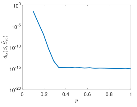
(a)

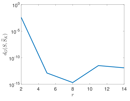
(b)

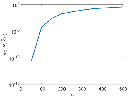
(c)

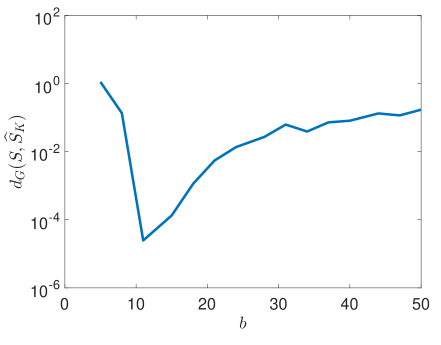
(d)

Figure 3: Performance of $\operatorname{SNIPE}$ as (a) sampling probability $p$, (b) subspace dimension $r$, (c) ambient dimension $n$, (d) block size $b$ vary. $\widehat{\mathcal{S}}_{K}$ is the output of $\operatorname{SNIPE}$ and $d_{G}(\mathcal{S},\widehat{\mathcal{S}}_{K})$ is its distance to the true subspace $\mathcal{S}$, which generated the input of $\operatorname{SNIPE}$. See Section 6 for details and note that each panel is generated with a different and random subspace $\mathcal{S}$.

Comparisons

Next we empirically compare $\operatorname{SNIPE}$ with $\operatorname{GROUSE}$ [24, 35], PETRELS [20], and the modified power method in [16]. In addition to the version of $\operatorname{SNIPE}$ given in Algorithm 1, we also include comparisons with a simple variant of $\operatorname{SNIPE}$, which we call $\operatorname{SNIPE-overlap}$. Unlike $\operatorname{SNIPE}$ which processes disjoint blocks, $\operatorname{SNIPE-overlap}$ processes all overlapping blocks of data. More precisely, for a block size $b$, $\operatorname{SNIPE-overlap}$ first processes data columns $t=1,2,...,b$, followed by columns $t=2,3,...,b+1$, and so on, whereas regular $\operatorname{SNIPE}$ processes columns $t=1,2,...,b$ followed by $t=b+1,b+2,...,2b$, etc. The theory developed in this paper does not hold for $\operatorname{SNIPE-overlap}$ because of lack of statistical independence between iterations, but we include the algorithm in the comparisons since it represents a minor modifications of the $\operatorname{SNIPE-overlap}$ framework and appears to have some empirical benefits, as detailed below.

In these experiments, we set $n=100$, $r=5$, $T=5000$, and take $\mathcal{S}\subset\mathbb{R}^{n}$ to be a generic $r$-dimensional subspace and simulate noiseless data samples as before. In Figure 4 we compare the algorithms for three values of sampling probability $p$, which shows the average over $100$ trials of the estimation error of algorithms (with respect to the metric $d_{\mathbb{G}}$) relative to the number of revealed data columns. For $\operatorname{SNIPE}$, we used the block size of $b=2r$. Having tried to get the best performance from $\operatorname{GROUSE}$, we used the “greedy” step-size as proposed in [35]. For [16], we set the block size as $b=1000$ which was found empirically to yield the lowest subspace error after $T=5000$ iterations.

In Table 1 we also compare the average number of revealed columns needed to reach a given error tolerance for each algorithm (as measured by error metric $d_{\mathbb{G}}$) for various values of the sampling probability $p$. We omit the modified power method from the results since it was unable to reach the given error tolerances in all cases. For the medium/high sampling rates $p=0.45,0.60,0.75$, $\operatorname{SNIPE-overlap}$ is fastest to converge, while regular $\operatorname{SNIPE}$ is competitive with $\operatorname{GROUSE}$ and $\operatorname{PETRELS}$. For the lower sampling rates $p=0.15,0.30$ we find $\operatorname{GROUSE}$ yields the fastest convergence, although $\operatorname{SNIPE-overlap}$ is also competitive with $\operatorname{GROUSE}$ for $p=0.30$.

$p=0.15$ $p=0.30$ $p=0.45$ $p=0.60$ $p=0.75$ $d_{\mathbb{G}}<10^{-3}$ $d_{\mathbb{G}}<10^{-7}$ $d_{\mathbb{G}}<10^{-3}$ $d_{\mathbb{G}}<10^{-7}$ $d_{\mathbb{G}}<10^{-3}$ $d_{\mathbb{G}}<10^{-7}$ $d_{\mathbb{G}}<10^{-3}$ $d_{\mathbb{G}}<10^{-7}$ $d_{\mathbb{G}}<10^{-3}$ $d_{\mathbb{G}}<10^{-7}$ GROUSE 878.0 (76.1) 1852.4 (85.2) 294.9 (20.6) 646.1 (26.8) 181.6 (13.8) 391.2 (18.0) 130.2 (10.3) 277.2 (12.8) 105.1 (11.7) 213.5 (12.8) PETRELS 1689.0 (1394.1) 2853.7 (916.9) 421.8 (31.3) 1100.5 (64.2) 262.1 (25.3) 802.0 (31.1) 181.8 (20.2) 671.4 (22.8) 133.3 (21.3) 599.1 (24.0) SNIPE 1815.7 (137.9) 3946.9 (182.4) 537.4 (39.9) 1236.4 (62.5) 282.4 (25.8) 649.6 (41.5) 171.4 (17.2) 391.4 (25.4) 105.5 (9.1) 241.6 (15.6) SNIPE-overlap 1588.3 (183.8) 3319.5 (232.9) 318.7 (27.1) 704.6 (36.8) 131.8 (11.6) 296.4 (17.4) 71.3 (5.7) 155.6 (9.9) 44.2 (4.2) 91.8 (6.8)

Table 1: Average number of revealed data columns needed to reach the indicated subspace recovery error for various sampling probabilities $p$ over 100 random trials. Standard deviations are given in parenthesis.

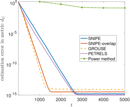
(a) $p=0.30$

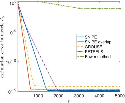
(b) $p=0.45$

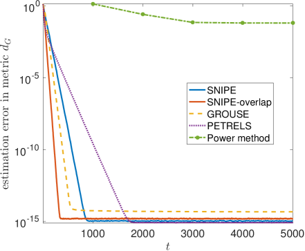
(c) $p=0.60$

Figure 4: Average subspace estimation error versus number of revealed data columns at the specified sampling probability $p$, see Section 6 for details.

7 Theory

In this section, we prove the technical results presented in Section 4. A short word on notation is in order first. We will frequently use MATLAB’s matrix notation so that, for example, $A[i,j]$ is the $[i,j]$th entry of $A$, and the row-vector $A[i,:]$ corresponds to the $i$th row of $A$. By $\{\epsilon_{i}\}_{i}\overset{\operatorname{ind.}}{\sim}\mbox{Bernoulli}(p)$, we mean that $\{\epsilon_{i}\}_{i}$ are independent Bernoulli random variables taking one with probability of $p$ and zero otherwise. Throughout, $E_{i,j}$ stands for the $[i,j]$th canonical matrix so that $E_{i,j}[i,j]=1$ is its only nonzero entry. The size of $E_{i,j}$ may be inferred from the context. As usual, $\|\cdot\|$ and $\|\cdot\|_{F}$ stand for the spectral and Frobenius norms. In addition, $\|A\|_{\infty}$ and $\|A\|_{2\rightarrow\infty}$ return the largest entry of a matrix $A$ (in magnitude) and the largest $\ell_{2}$ norm of the rows of $A$, respectively. Singular values of a matrix $A$ are denoted by $\sigma_{1}(A)\geq\sigma_{2}(A)\geq\cdots$. For purely aesthetic reasons, we will occasionally use the notation $a\vee b=\max(a,b)$ and $a\wedge b=\min(a,b)$.

7.1 Convergence of SNIPE to a Stationary Point (Proof of Theorem 1)

Consider Program (2), namely

$$\begin{cases}\min\,\,\,f_{\Omega}\left(X,\mathcal{U}\right):=\|P_{\mathcal{U}}^{\perp}X\|_{F}^{2}+\lambda\|P_{\Omega^{C}}(X)\|_{F}^{2},\\ P_{\Omega}(X)=Y,\end{cases}$$ (30)

where the minimization is over matrix $X\in\mathbb{R}^{n\times T}$ and subspace $\mathcal{U}\in\mathbb{G}(n,r)$. Before proceeding with the rest of the proof, let us for future reference record the partial derivatives of $f_{\Omega}$ below. Consider a small perturbation to $X$ in the form of $X+\Delta$, where $\Delta\in\mathbb{R}^{n\times T}$. Let $U\in\mathbb{R}^{n\times r}$ and $U^{\perp}$ be orthonormal bases for $\mathcal{U}$ and its orthogonal complement $\mathcal{U}^{\perp}$, respectively. Consider also a small perturbation to $U$ in the form of $U+U^{\perp}\Delta^{\prime}\in\mathbb{R}^{n\times r}$, where $\Delta^{\prime}\in\mathbb{R}^{(n-r)\times r}$. The perturbation to $f_{\Omega}(X,\mathcal{U})=f_{\Omega}(X,U)$ can be written as

$$f_{\Omega}\left(X+\Delta,U+U^{\perp}\Delta^{\prime}\right)=f_{\Omega}\left(X,\mathcal{U}\right)+\left\langle\Delta,\partial_{X}f_{\Omega}\left(X,\mathcal{U}\right)\right\rangle+\left\langle\Delta^{\prime},\partial_{\mathcal{U}}f_{\Omega}\left(X,\mathcal{U}\right)\right\rangle+o(\|\Delta\|_{F})+o(\|\Delta^{\prime}\|_{F}),$$ (31)

where $o(\cdot)$ is the standard little-$o$ notation. The partial derivatives of $f_{\Omega}$ are listed below and derived in Appendix D.

Lemma 5.

For $f_{\Omega}$ in Program (30), the first-order partial derivatives at $(X,\mathcal{U})\in\mathbb{R}^{n\times T}\times\mathbb{G}(n,r)$ are

$$\partial_{X}f_{\Omega}\left(X,\mathcal{U}\right)=2P_{\mathcal{U}^{\perp}}X+2\lambda P_{\Omega^{C}}(X)\in\mathbb{R}^{n\times T},\qquad\partial_{\mathcal{U}}f_{\Omega}\left(X,\mathcal{U}\right)=-2(U^{\perp})^{*}XX^{*}U\in\mathbb{R}^{(n-r)\times r},$$ (32)

where $U\in\mathbb{R}^{n\times r}$ and $U^{\perp}\in\mathbb{R}^{n\times(n-r)}$ are orthonormal bases for $\mathcal{U}$ and its orthogonal complement, respectively.

Recall that $Q_{k}\in\mathbb{R}^{r\times b}$ is a random matrix with bounded expectation, namely $\mathbb{E}\|\mathcal{Q}_{k}\|_{F}<\infty$. As $K\rightarrow\infty$, $\{Q_{k}\}_{k=1}^{K}$ therefore has a bounded subsequence. To keep the notation simple and without any loss of generality, we assume that in fact the sequence $\{Q_{k}\}_{k}$ is itself bounded. As $K\rightarrow\infty$ and for an integer $l$, we can always find an interval of length $l$ over which the same index set and nearly the same coefficient matrix repeats. More specifically, consider an index set $\widehat{\Omega}\subseteq[1:n]\times[1:b]$ and a matrix $\widehat{Q}\in\mathbb{R}^{r\times b}$ in the support of the distributions from which $\{\Omega_{k}\}_{k=1}^{K}$ and $\{Q_{k}\}_{k=1}^{K}$ are drawn. For every integer $l$, as a result of the second Borel-Cantelli lemma [36, pg. 64], almost surely there exists a contiguous interval

$$\kappa_{l}:=[k_{l}-l+1:k_{l}],$$ (33)

such that

$$\Omega_{k}=\widehat{\Omega},\qquad k\in\kappa_{l},$$ (34)

$$\max_{k\in\kappa_{l}}\|Q_{k}-\widehat{Q}\|_{F}\leq\frac{1}{l}.$$ (35)

As $l\rightarrow\infty$, the measurements corresponding to the interval $\kappa_{l}$ converge. To be specific, let $\widehat{Y}:=P_{\widehat{\Omega}}(S\widehat{Q})$ and note that

$$\lim_{l\rightarrow\infty}\max_{k\in\kappa_{l}}\,\,\,\|Y_{k}-\widehat{Y}\|_{F} =\lim_{l\rightarrow\infty}\max_{k\in\kappa_{l}}\,\,\,\|P_{\Omega_{k}}(SQ_{k})-\widehat{Y}\|_{F}$$

$$=\lim_{l\rightarrow\infty}\max_{k\in\kappa_{l}}\,\,\,\|P_{\widehat{\Omega}}(SQ_{k})-\widehat{Y}\|_{F}$$

$$=\lim_{l\rightarrow\infty}\max_{k\in\kappa_{l}}\,\,\,\|P_{\widehat{\Omega}}(S(Q_{k}-\widehat{Q}))\|_{F}$$

$$\leq\lim_{l\rightarrow\infty}\max_{k\in\kappa_{l}}\,\,\,\|Q_{k}-\widehat{Q}\|_{F}$$

$$=0.$$ (36)

The above observation encourages us to exchange $(\Omega_{k},Y_{k})$ with $(\widehat{\Omega},\widehat{Y})$ on the interval $\kappa_{l}$. Let us therefore study the program

$$\begin{cases}\min\,\,\,f_{\widehat{\Omega}}(X,\mathcal{U}),\\ P_{\widehat{\Omega}}(X)=\widehat{Y},\end{cases}$$ (37)

where the minimization is over all matrices $X\in\mathbb{R}^{n\times b}$ and subspaces $\mathcal{U}\in\mathbb{G}(n,r)$. From a technical viewpoint, it is in fact more convenient to relax the equality constraint above as

$$\begin{cases}\min\,\,\,f_{\widehat{\Omega}}(X,\mathcal{U}),\\ \|P_{\widehat{\Omega}}(X)-\widehat{Y}\|_{F}\leq\epsilon,\end{cases}$$ (38)

for $\epsilon>0$. We fix $\epsilon$ for now. Let us next use alternative minimization to solve Program (38). More specifically, recall (33) and consider the initialization $\widehat{\mathcal{S}}_{k_{l}-l,\epsilon}:=\widehat{\mathcal{S}}_{k_{l}-l}$, where $\widehat{\mathcal{S}}_{k_{l}-l}$ is the output of $\operatorname{SNIPE}$ at iteration $k_{l}-l$, see Algorithm 1. For every $k\in\kappa_{l}$, consider the program

$$\begin{cases}\min\,\,\,f_{\widehat{\Omega}}(X,\widehat{\mathcal{S}}_{k-1,\epsilon}),\\ \|P_{\widehat{\Omega}}(X)-\widehat{Y}\|_{F}\leq\epsilon,\end{cases}$$ (39)

and let $R_{k,\epsilon}$ be a minimizer of Program (39). We then update the subspace by solving

$$\underset{\mathcal{U}\in\mathbb{G}(n,r)}{\min}\,\,\,f_{\widehat{\Omega}}(R_{k,\epsilon},\mathcal{U}),\\$$ (40)

and setting $\widehat{\mathcal{S}}_{k,\epsilon}$ to be a minimizer of Program (40). Recalling the definition of $f_{\widehat{\Omega}}$ in Program (30) and in light of the Eckart-Young-Mirsky Theorem, Program (40) can be solved by computing top $r$ left singular vectors of $R_{k,\epsilon}$ [8, 9]. For future reference, note that the optimality and hence stationarity of $\widehat{\mathcal{S}}_{k,\epsilon}$ in Program (40) dictates that

$$\partial_{\mathcal{U}}f_{\widehat{\Omega}}(R_{k,\epsilon},\widehat{\mathcal{S}}_{k,\epsilon})=0,\qquad k\in\kappa_{l},$$ (41)

where $\partial_{\mathcal{U}}f$ was specified in Lemma 5. From the above construction of the sequence $\{(R_{k,\epsilon},\widehat{\mathcal{S}}_{k,\epsilon})\}_{k\in\kappa_{l}}$, we also observe that

$$0\leq f_{\widehat{\Omega}}(R_{k,\epsilon},\widehat{\mathcal{S}}_{k,\epsilon})\leq f_{\widehat{\Omega}}(R_{k,\epsilon},\widehat{\mathcal{S}}_{k-1,\epsilon})\leq f_{\widehat{\Omega}}(R_{k-1,\epsilon},\widehat{\mathcal{S}}_{k-1,\epsilon}),$$ (42)

for every $k\in[k_{l}-l+2:k_{l}]\subset\kappa_{l}$, see (33). That is, $\{f_{\widehat{\Omega}}(R_{k,\epsilon},\widehat{\mathcal{S}}_{k,\epsilon})\}_{k\in\kappa_{l}}$ is a nonincreasing and nonnegative sequence. It therefore holds that

$$\lim_{l\rightarrow\infty}\left|f_{\widehat{\Omega}}(R_{k_{l}-1,\epsilon},\widehat{\mathcal{S}}_{k_{l}-1,\epsilon})-f_{\widehat{\Omega}}(R_{k_{l},\epsilon},\widehat{\mathcal{S}}_{k_{l}-1,\epsilon})\right|=0.$$ (43)

By the feasibility of $R_{k_{l}-1,\epsilon}$ in Program (39) and by the continuity of $f_{\widehat{\Omega}}(X,\mathcal{U})$ in $X$, we conclude in light of (43) that $R_{k_{l}-1,\epsilon}$ too is a minimizer (and hence also a stationary point) of Program (39) and in the limit of $l\rightarrow\infty$. We therefore find by writing the stationarity conditions of Program (39) at $R_{k_{l},\epsilon}$ that

$$\|P_{\widehat{\Omega}}(R_{k_{l},\epsilon})-\widehat{Y}\|_{F}\leq\epsilon,$$ (44)

$$\lim_{l\rightarrow\infty}\left\|\partial_{X}f_{\widehat{\Omega}}(R_{k_{l},\epsilon},\widehat{\mathcal{S}}_{k_{l},\epsilon})+\lambda_{k_{l},\epsilon}(P_{\widehat{\Omega}}(R_{k_{l},\epsilon})-\widehat{Y})\right\|_{F}=0.$$ (45)

for nonnegative $\lambda_{k_{l},\epsilon}$. Recalling the definition of $f_{\widehat{\Omega}}$ and that $\lambda>0$ by assumption, we observe that Program (39) is strongly convex in $P_{\widehat{\Omega}^{C}}(X)$ and consequently any pair of minimizers of Program (39) must agree on the index set $\widehat{\Omega}^{C}$. Optimality of $R_{k_{l},\epsilon}$ and limit optimality of $R_{k_{l}-1,\epsilon}$ in Program (39) therefore imply that

$$\lim_{l\rightarrow\infty}\left\|P_{\widehat{\Omega}^{C}}(R_{k_{l}-1,\epsilon}-R_{k_{l},\epsilon})\right\|_{F}=0.$$ (46)

On the index set $\widehat{\Omega}$, on the other hand, the feasibility of both $R_{k_{l}-1,\epsilon}$ and $R_{k_{l},\epsilon}$ in Program (39) implies that

$$\|P_{\widehat{\Omega}}(R_{k_{l}-1,\epsilon}-R_{k_{l},\epsilon})\|_{F} \leq\|P_{\widehat{\Omega}}(R_{k_{l}-1,\epsilon})-\widehat{Y}\|_{F}+\|P_{\widehat{\Omega}}(R_{k_{l},\epsilon})-\widehat{Y}\|_{F}\qquad\mbox{(triangle inequality)}$$

$$\leq 2\epsilon.$$ (47)

Combining (46) and (47) yields that

$$\lim_{l\rightarrow\infty}\|R_{k_{l}-1,\epsilon}-R_{k_{l},\epsilon}\|_{F}$$

$$\leq\lim_{l\rightarrow\infty}\|P_{\widehat{\Omega}}(R_{k_{l}-1,\epsilon}-R_{k_{l},\epsilon})\|_{F}+\lim_{l\rightarrow\infty}\|P_{\widehat{\Omega}^{C}}(R_{k_{l}-1,\epsilon}-R_{k_{l},\epsilon})\|_{F}\qquad\mbox{(triangle inequality)}$$

$$\leq 2\epsilon,\qquad\mbox{(see (\ref{eq:cauchy 1},\ref{eq:cauchy 2}))}$$ (48)

In light of (39), $\{R_{k_{l},\epsilon}\}_{l}$ is bounded and consequently has a convergent subsequence. Without loss of generality and to simplify the notation, we assume that $\{R_{k_{l},\epsilon}\}_{l}$ is itself convergent, namely that there exists $R_{\epsilon}\in\mathbb{R}^{n\times b}$ for which

$$\lim_{l\rightarrow\infty}\|R_{k_{l},\epsilon}-R_{\epsilon}\|_{F}\leq 2\epsilon.$$ (49)

Let us now send $\epsilon$ to zero in (49) to obtain that

$$\lim_{\epsilon\rightarrow 0}\lim_{l\rightarrow\infty}\|R_{k_{l},\epsilon}-R_{\epsilon}\|_{F}\leq\lim_{\epsilon\rightarrow 0}2\epsilon=0.$$ (50)

We next show that it is possible to essentially change the order of limits above and also conclude that $(R,\widehat{\mathcal{S}})$ coincides with the output of $\operatorname{SNIPE}$ in limit. The following result is proved in Appendix E.

Lemma 6.

With the setup above, there exist a sequence $\{\epsilon_{i}\}_{i}$ with $\lim_{i\rightarrow\infty}\epsilon_{i}=0$ and a matrix $R\in\mathbb{R}^{n\times b}$ such that

$$\lim_{l,i\rightarrow\infty}\|R_{k_{l},\epsilon_{i}}-R\|_{F} =\lim_{l\rightarrow\infty}\lim_{i\rightarrow\infty}\|R_{k_{l},\epsilon_{i}}-R\|_{F}$$

$$=\lim_{i\rightarrow\infty}\lim_{l\rightarrow\infty}\|R_{k_{l},\epsilon_{i}}-R\|_{F}$$

$$=0.$$ (51)

Moreover, suppose that the output of $\operatorname{SNIPE}$ in every iteration has a spectral gap in the sense that there exists $\tau>0$ such that

$$\frac{\sigma_{r}(R_{k})}{\sigma_{r+1}(R_{k})}\geq 1+\tau,$$ (52)

for every $k$. Let $\widehat{\mathcal{S}}_{k_{l},\epsilon_{i}}$ and $\widehat{\mathcal{S}}$ be the span of top $r$ left singular vectors of $R_{k_{l},\epsilon_{i}}$ and $R$, respectively. Then it holds that

$$\lim_{l,i\rightarrow\infty}d_{\mathbb{G}}(\widehat{\mathcal{S}}_{k_{l},\epsilon_{i}},\mathcal{S})=0.$$ (53)

Lastly, in the limit of $l\rightarrow\infty$, $\operatorname{SNIPE}$ produces $(R,\widehat{\mathcal{S}})$ in every iteration, namely

$$\lim_{l\rightarrow\infty}\|R_{k_{l}}-R\|_{F}=\lim_{l\rightarrow\infty}d_{\mathbb{G}}(\widehat{\mathcal{S}}_{k_{l}},\widehat{\mathcal{S}})=0,$$ (54)

where $(R_{k_{l}},\widehat{\mathcal{S}}_{k_{l}})$ is the output of $\operatorname{SNIPE}$ in iteration $k_{l}$, see Algorithm 1.

In fact, the pair $(R,\widehat{S})$ from Lemma 6 is stationary in limit in the sense described next and proved in Appendix F.

Lemma 7.

The pair $(R,\widehat{S})$ in Lemma 6 is a stationary point of the program

$$\begin{cases}\min\,\,\,f_{\Omega_{k_{l}}}(X,\mathcal{U}),\\ P_{\Omega_{k_{l}}}(X)=Y_{k_{l}},\end{cases}$$ (55)

as $l\rightarrow\infty$. The minimization above is over all matrices $X\in\mathbb{R}^{n\times b}$ and subspaces $\mathcal{U}\in\mathbb{G}(n,r)$. More specifically, it holds that

$$\lim_{l\rightarrow\infty}\|\partial_{\mathcal{U}}f_{\Omega_{k_{l}}}(R,\widehat{\mathcal{S}})\|_{F}=0,$$ (56)

$$\lim_{l\rightarrow\infty}\|P_{{\Omega}_{k_{l}}}(R)-{Y}_{k_{l}}\|_{F}=0,$$ (57)

$$\lim_{l\rightarrow\infty}\|P_{{\Omega}_{k_{l}}^{C}}(\partial_{X}f_{\Omega_{k_{l}}}(R,\widehat{\mathcal{S}}))\|_{F}=0.$$ (58)

In words, Lemmas 6 and 7 together imply that the output of $\operatorname{SNIPE}$ in limit is a stationary point of Program (55). This completes the proof of Theorem 1.

7.2 Convergence of SNIPE (Proof of Proposition 2)

In iteration $k$ of $\operatorname{SNIPE}$, we partially observe the data block $SQ_{k}\in\mathbb{R}^{n\times b}$ on a random index set $\Omega_{k}\subset[1:n]\times[1:b]$, where $Q_{k}\in\mathbb{R}^{r\times b}$ is a random coefficient matrix. We collect the observations in $Y_{k}=P_{\Omega_{k}}(SQ_{k})\in\mathbb{R}^{n\times b}$, see Sections 2 and 3 for the detailed setup. Note that $R_{k}$ in (1) can be written as

$$R_{k}=Y_{k}+P_{\Omega_{k}^{C}}(\widehat{S}_{k-1}Q^{\prime}_{k})=P_{\Omega_{k}}(SQ_{k})+P_{\Omega_{k}^{C}}(\widehat{S}_{k-1}Q^{\prime}_{k}),$$ (59)

where

$$Q^{\prime}_{k}:=\left[\begin{array}[]{ccc}\cdots&\left(\widehat{S}_{k-1}^{*}P_{\omega_{t}}\widehat{S}_{k-1}+\lambda I_{r}\right)^{\dagger}y_{t}&\cdots\end{array}\right]\in\mathbb{R}^{r\times b}.$$ (60)

By (13), there exists $Q^{\prime\prime}_{k}\in\mathbb{R}^{r\times b}$ and

$$R^{\prime}_{k}:=P_{\Omega_{k}}(SQ_{k})+P_{\Omega_{k}^{C}}(\widehat{S}Q^{\prime\prime}_{k}),$$ (61)

such that

$$\lim_{k\rightarrow\infty}\|R_{k}-R^{\prime}_{k}\|_{F}=0.$$ (62)

In (61) above, $\widehat{S}\in\mathbb{R}^{n\times r}$ is an orthonormal basis for the subspace $\widehat{\mathcal{S}}$. In Algorithm 1, the rank-$r$ truncated SVD of $R_{k}$ spans $\widehat{\mathcal{S}}_{k}\in\mathbb{G}(n,r)$, namely the output of $\operatorname{SNIPE}$ in iteration $k$. Let also $\widehat{\mathcal{S}}^{\prime}_{k}\in\mathbb{G}(n,r)$ denote the span of rank-$r$ truncated SVD of $R^{\prime}_{k}$. The existence of the reject option in Algorithm 1 with positive $\tau$ implies that $R_{k}$ has a spectral gap and therefore $\widehat{\mathcal{S}}_{k}$ is uniquely defined. Combining this with (62), we find that $\widehat{\mathcal{S}}_{k}^{\prime}$ too is uniquely defined in the limit of $k\rightarrow\infty$. Therefore another consequence of (62) is that

$$\lim_{k\rightarrow\infty}d_{\mathbb{G}}(\widehat{\mathcal{S}}_{k},\widehat{\mathcal{S}}_{k}^{\prime})=0.$$ (63)

Then we have that

$$\lim_{k\rightarrow\infty}d_{\mathbb{G}}(\widehat{\mathcal{S}}^{\prime}_{k},\widehat{\mathcal{S}}) \leq\lim_{k\rightarrow\infty}d_{\mathbb{G}}(\widehat{\mathcal{S}}_{k}^{\prime},\widehat{\mathcal{S}}_{k})+\lim_{k\rightarrow\infty}d_{\mathbb{G}}(\widehat{\mathcal{S}}_{k},\widehat{\mathcal{S}})$$

$$\leq 0+0,\qquad\mbox{(see (\ref{eq:RnRprime subspaces},\ref{eq:limExists}))}$$ (64)

namely, $\widehat{\mathcal{S}}^{\prime}_{k}$ converges to $\widehat{\mathcal{S}}$ in the limit too. Let us now rewrite $R^{\prime}_{k}$ as

$$R^{\prime}_{k}=P_{\Omega_{k}}(SQ_{k}-\widehat{S}Q^{\prime\prime}_{k})+\widehat{S}Q^{\prime\prime}_{k},\qquad\mbox{(see \eqref{eq:def of Rprime})}$$ (65)

which, together with (64), implies that

$$\lim_{k\rightarrow\infty}\|\widehat{S}^{*}P_{\Omega_{k}}(SQ_{k}-\widehat{S}Q^{\prime\prime}_{k})\|_{F}=0.$$ (66)

We can rewrite the above limit in terms of the data vectors (rather than data blocks) to obtain that

$$\lim_{t\rightarrow\infty}\|\widehat{S}^{*}P_{\omega_{t}}(Sq_{t}-\widehat{S}q^{\prime\prime}_{t})\|_{F}=0,$$ (67)

where $\{q_{t},q^{\prime\prime}_{t}\}_{t}$ form the columns of the blocks $\{Q_{k},Q^{\prime\prime}_{k}\}_{k}$, and the index sets $\{\omega_{t}\}_{t}\subseteq[1:n]$ form $\{\Omega_{k}\}_{k}$. There almost surely exists a subsequence $\{t_{i}\}_{i}$ over which $\omega_{t_{i}}=\{1\}$, namely there is a subsequence where we only observe the first entry of the incoming data vector. Consider a vector $q^{1}\in\mathbb{R}^{r}$ in the support of the distribution from which $\{q_{t}\}_{t}$ are drawn. Then there also exists a subsequence of $\{t_{i}\}_{i}$, denoted by $\{t_{i_{j}}\}_{i_{j}}$, such that $\lim_{j\rightarrow\infty}\|q_{t_{i_{j}}}-q^{1}\|_{2}=0$. Restricted to the subsequence $\{t_{i_{j}}\}_{j}$, (67) reads as

$$0 =\lim_{j\rightarrow\infty}\|\widehat{S}^{*}P_{\omega_{t_{i_{j}}}}(Sq_{t_{i_{j}}}-\widehat{S}q^{\prime\prime}_{t_{i_{j}}})\|_{F}$$

$$=\lim_{j\rightarrow\infty}\|\widehat{S}^{*}P_{\{1\}}(Sq_{t_{i_{j}}}-\widehat{S}q^{\prime\prime}_{t_{i_{j}}})\|_{F}$$

$$=\|\widehat{S}^{*}P_{\{1\}}(Sq^{1}-\widehat{S}q^{\prime\prime 1})\|_{F},$$ (68)

where we set $q^{\prime\prime 1}:=\lim_{j\rightarrow\infty}q^{\prime\prime}_{t_{i_{j}}}$; the limit exists by (60). Likewise, we can show that

$$v^{l}:=P_{\{l\}}(Sq^{l}-\widehat{S}q^{\prime\prime l})\in\mathcal{S}^{\perp},\qquad l\in[1:n],$$ (69)

where $\{q^{\prime\prime l}\}_{l}$ are defined similarly. Because $\dim(\mathcal{S}^{\perp})=n-r$, at most $n-r$ of the vectors $\{v^{l}\}_{l=1}^{n}$ are linearly independent. Because the supports of $\{v^{l}\}_{l}$ are disjoint, it follows that there are at most $n-r$ of the vectors $\{v^{l}\}_{l=1}^{n}$ are nonzero. Put differently, there exists an index set $I\subset[1:n]$ of size at least $r$ such that

$$Sq^{l}=\widehat{S}q^{\prime\prime l},\qquad l\in I.$$ (70)

Almost surely, $\{q^{l}\}_{l\in I}\subset\mathbb{R}^{r}$ form a basis for $\mathbb{R}^{r}$, and therefore $\mathcal{S}\subseteq\widehat{\mathcal{S}}$. Because $\widehat{\mathcal{S}}\in\mathbb{G}(n,r)$ by assumption, it follows that $\widehat{\mathcal{S}}=\mathcal{S}$, which completes the proof of Proposition 2.

7.3 Locally Linear Convergence of SNIPE (Proof of Theorems 3 and 4)

At iteration $k\in[2:K]$, $\operatorname{SNIPE}$ uses the current estimate $\widehat{\mathcal{S}}_{k-1}$ and the new incomplete block $Y_{k}$ to produce a new estimate $\widehat{\mathcal{S}}_{k}$ of the true subspace $\mathcal{S}$. The main challenge here is to compare the new and old principal angles with $\mathcal{S}$, namely compare $d_{\mathbb{G}}(\mathcal{S},\widehat{\mathcal{S}}_{k})$ and $d_{\mathbb{G}}(\mathcal{S},\widehat{\mathcal{S}}_{k-1})$. Lemma 8 below, proved in Appendix G, loosely speaking states that $d_{\mathbb{G}}(\mathcal{S},\widehat{\mathcal{S}}_{k})$ reduces by a factor of $1-O(p)$ in expectation in every iteration, when $d_{\mathbb{G}}(\mathcal{S},\widehat{\mathcal{S}}_{k})\lesssim p^{\frac{5}{2}}$ and ignoring all other parameters in this qualitative discussion. In other words, when sufficiently small, the estimation error of $\operatorname{SNIPE}$ reduces in every iteration, but in expectation. The actual behavior of $\operatorname{SNIPE}$ is more nuanced. Indeed, Lemma 8 below also adds that the estimation error $d_{\mathbb{G}}(\mathcal{S},\widehat{\mathcal{S}}_{k})$ in fact contracts in some iterations by a factor of ${1-Cp}$, namely

$$d_{\mathbb{G}}(\mathcal{S},\widehat{\mathcal{S}}_{k})\lesssim({1-Cp})\cdot d_{\mathbb{G}}(\mathcal{S},\widehat{\mathcal{S}}_{k-1}),$$

provided that $d_{\mathbb{G}}(\mathcal{S},\widehat{\mathcal{S}}_{k-1})\lesssim p^{\frac{5}{2}}$. That is, when sufficiently small, the estimation error of $\operatorname{SNIPE}$ reduces in some but not all iterations. In the rest of iterations, the error does not increase by much, namely

$$d_{\mathbb{G}}(\mathcal{S},\widehat{\mathcal{S}}_{k})\approx d_{\mathbb{G}}(\mathcal{S},\widehat{\mathcal{S}}_{k-1}),$$

with high probability and provided that $d_{\mathbb{G}}(\mathcal{S},\widehat{\mathcal{S}}_{k-1})\lesssim p^{\frac{5}{2}}$.

Lemma 8.

Fix $k\in[2:K]$, $\alpha,\nu\geq 1$, and $c>0$. Let $\mathfrak{E}_{k-1}$ be the event where

$$p\gtrsim\alpha^{2}\log^{2}b\log n\frac{\eta(\widehat{\mathcal{S}}_{k-1})r}{n},$$ (71)

$$d_{\mathbb{G}}(\mathcal{S},\widehat{\mathcal{S}}_{k-1})\lesssim\frac{p^{\frac{7}{2}}nb}{\alpha c\log b\sqrt{r\log n}},$$ (72)

and let $\mathfrak{E}^{\prime}_{k}$ be the event where $\|Q_{k}\|\leq\nu\cdot\sigma_{\min}$, where $\sigma_{\min}$ is the reject threshold in $\operatorname{SNIPE}$, see Algorithm 1. Then it holds that

$$\mathbb{E}\left[d_{\mathbb{G}}(\mathcal{S},\widehat{\mathcal{S}}_{k})\,|\,\widehat{\mathcal{S}}_{k-1},\mathfrak{E}_{k-1},\mathfrak{E}^{\prime}_{k}\right] \leq\nu\left(1-\frac{p}{2}+\frac{p^{3}nb}{c}\right)d_{\mathbb{G}}(\mathcal{S},\widehat{\mathcal{S}}_{k-1})+\frac{b^{-C\alpha}}{\sqrt{r}}.$$ (73)

Moreover, conditioned on $\widehat{\mathcal{S}}_{k-1}$ and the event $\mathfrak{E}_{k-1}\cap\mathfrak{E}^{\prime}_{k}$, it holds that

$$d_{\mathbb{G}}(\mathcal{S},\widehat{\mathcal{S}}_{k})\leq\nu\left(1+\frac{p^{3}nb}{c}\right)d_{\mathbb{G}}(\mathcal{S},\widehat{\mathcal{S}}_{k-1}),$$ (74)

except with a probability of at most $b^{-C\alpha}$. Lastly, a stronger bound holds conditioned on $\widehat{\mathcal{S}}_{k-1}$ and the event $\mathfrak{E}_{k-1}\cap\mathfrak{E}^{\prime}_{k}$, namely

$$d_{\mathbb{G}}(\mathcal{S},\widehat{\mathcal{S}}_{k})\leq\nu\left(1-\frac{p}{4}+\frac{p^{3}nb}{c}\right)d_{\mathbb{G}}(\mathcal{S},\widehat{\mathcal{S}}_{k-1})$$ (75)

with a probability of at least

$$\phi_{k}(\alpha):=1-\exp\left(-\frac{\Cl{fail}p^{2}nb}{\widetilde{\eta}_{k-1}}\right)-b^{-C\alpha},$$ (76)

where

$$\widetilde{\eta}_{k}=\widetilde{\eta}(P_{\widehat{\mathcal{S}}_{k-1}^{\perp}}S_{k}):=nb\cdot\frac{\|P_{\widehat{\mathcal{S}}_{k-1}^{\perp}}S_{k}\|^{2}_{\infty}}{\|P_{\widehat{\mathcal{S}}_{k-1}^{\perp}}S_{k}\|_{F}^{2}}.$$ (77)

Let us now use Lemma 8 to complete the proofs of Theorems 3 and 4.

7.3.1 Proof of Theorem 3

With the choice of $c=4p^{2}nb$ and $\nu=1/\sqrt{1-p/4}$, (73) reads as

$$\mathbb{E}\left[d_{\mathbb{G}}(\mathcal{S},\widehat{\mathcal{S}}_{k})\,|\,\widehat{\mathcal{S}}_{k-1},\mathfrak{E}_{k-1},\mathfrak{E}^{\prime}_{k}\right] \leq\nu\left(1-\frac{p}{2}+\frac{p^{3}nb}{c}\right)d_{\mathbb{G}}(\mathcal{S},\widehat{\mathcal{S}}_{k-1})+\frac{b^{-C\alpha}}{\sqrt{r}}\qquad\mbox{(see \eqref{eq:dragon in exp})}$$

$$=\sqrt{1-\frac{p}{4}}d_{\mathbb{G}}(\mathcal{S},\widehat{\mathcal{S}}_{k-1})+\frac{b^{-C\alpha}}{\sqrt{r}}$$

$$\leq\left(1-\frac{p}{8}\right)d_{\mathbb{G}}(\mathcal{S},\widehat{\mathcal{S}}_{k-1})+\frac{b^{-C\alpha}}{\sqrt{r}}.$$ (78)

With the choice of

$$\alpha=-\frac{C\log\left(p\sqrt{r}d_{\mathbb{G}}(\mathcal{S},\widehat{\mathcal{S}}_{k-1})/16\right)}{\log b},$$ (79)

for an appropriate constant $C$ above, the bound in (78) simplifies to

$$\mathbb{E}\left[d_{\mathbb{G}}(\mathcal{S},\widehat{\mathcal{S}}_{k})\,|\,\widehat{\mathcal{S}}_{k-1},\mathfrak{E}_{k-1},\mathfrak{E}^{\prime}_{k}\right] \leq\left(1-\frac{p}{8}\right)d_{\mathbb{G}}(\mathcal{S},\widehat{\mathcal{S}}_{k-1})+\frac{b^{-C\alpha}}{\sqrt{r}}\qquad\mbox{(see \eqref{eq:exp proof pre})}$$

$$\leq\left(1-\frac{p}{8}\right)d_{\mathbb{G}}(\mathcal{S},\widehat{\mathcal{S}}_{k-1})+\frac{p}{16}d_{\mathbb{G}}(\mathcal{S},\widehat{\mathcal{S}}_{k-1})$$

$$\leq\left(1-\frac{p}{16}\right)d_{\mathbb{G}}(\mathcal{S},\widehat{\mathcal{S}}_{k-1}).$$ (80)

Lastly we remove the conditioning on $\mathfrak{E}^{\prime}_{k}$ above. Using the law of total expectation, we write that

$$\mathbb{E}\left[d_{\mathbb{G}}(\mathcal{S},\widehat{\mathcal{S}}_{k})\,|\,\widehat{\mathcal{S}}_{k-1},\mathfrak{E}_{k-1}\right]$$

$$=\mathbb{E}\left[d_{\mathbb{G}}(\mathcal{S},\widehat{\mathcal{S}}_{k})\,|\,\widehat{\mathcal{S}}_{k-1},\mathfrak{E}_{k-1},\mathfrak{E}^{\prime}_{k}\right]\cdot\Pr[\mathfrak{E}^{\prime}_{k}]+\mathbb{E}\left[d_{\mathbb{G}}(\mathcal{S},\widehat{\mathcal{S}}_{k})\,|\,\widehat{\mathcal{S}}_{k-1},\mathfrak{E}_{k-1},\mathfrak{E}^{\prime C}_{k}\right]\cdot\Pr[\mathfrak{E}^{\prime C}_{k}]$$

$$\leq\mathbb{E}\left[d_{\mathbb{G}}(\mathcal{S},\widehat{\mathcal{S}}_{k})\,|\,\widehat{\mathcal{S}}_{k-1},\mathfrak{E}_{k-1},\mathfrak{E}^{\prime}_{k}\right]+\Pr[\mathfrak{E}^{\prime C}_{k}]\qquad\mbox{(see \eqref{eq:err metric})}$$

$$\leq\left(1-\frac{p}{16}\right)d_{\mathbb{G}}(\mathcal{S},\widehat{\mathcal{S}}_{k-1})+\Pr[\mathfrak{E}^{\prime C}_{k}]\qquad\mbox{(see \eqref{eq:base cond})}$$

$$\leq\left(1-\frac{p}{32}\right)d_{\mathbb{G}}(\mathcal{S},\widehat{\mathcal{S}}_{k-1}),$$ (81)

where the last line holds if

$$\Pr[\mathfrak{E}^{\prime C}_{k}]\leq\frac{p}{32}d_{\mathbb{G}}(\mathcal{S},\widehat{\mathcal{S}}_{k-1}).$$

With the choice of $c,\nu,\alpha$ above, let us also rewrite the event $\mathfrak{E}_{k-1}$ in Lemma 8. First, we rewrite (72) as

$$d_{\mathbb{G}}(\mathcal{S},\widehat{\mathcal{S}}_{k-1}) \lesssim\frac{p^{\frac{7}{2}}nb}{\alpha c\log b\sqrt{r\log n}}$$

$$=\frac{Cp^{\frac{3}{2}}}{\alpha\log b\sqrt{r\log n}}$$

$$=-\frac{Cp^{\frac{3}{2}}}{\log\left(p\sqrt{r}d_{\mathbb{G}}(\mathcal{S},\widehat{\mathcal{S}}_{k-1})/16\right)\sqrt{r\log n}}.\qquad\mbox{(see \eqref{eq:choice of alpha exp})}$$ (82)

Second, we replace the coherence $\eta(\widehat{\mathcal{S}}_{k-1})$ in (71) with the simpler quantity $\eta(\mathcal{S})$. We can do so thanks to Lemma 12 which roughly speaking states that a pair of subspaces $\mathcal{A}$ and $\mathcal{B}$ with a small principal angle have similar coherences, namely $\theta_{1}(\mathcal{A},\mathcal{B})\approx 0\Longrightarrow\eta(\mathcal{A})\approx\eta(\mathcal{B})$. More concretely, note that

$$\sqrt{\eta(\widehat{\mathcal{S}}_{k-1})} \leq\sqrt{\eta\left(\mathcal{S}\right)}+d_{\mathbb{G}}(\mathcal{S},\widehat{\mathcal{S}}_{k-1})\sqrt{n}\qquad\mbox{(see Lemma \ref{lem:coherence perturbation})}$$

$$\leq\sqrt{\eta(\mathcal{S})}+Cp^{\frac{3}{2}}\sqrt{\frac{n}{r\log n}}\qquad\mbox{(see \eqref{eq:activate exp})}$$

$$\leq\sqrt{\eta(\mathcal{S})}+1\qquad\left(\mbox{if }p\lesssim\frac{1}{\sqrt{nb}}\right)$$

$$\leq 2\sqrt{\eta(\mathcal{S})}.\qquad\mbox{(see \eqref{eq:coh is bounded})}$$ (83)

This completes the proof of Theorem 3.

7.3.2 Proof of Theorem 4

For $K_{0}\in[1:K]$, we condition on $\widehat{\mathcal{S}}_{K_{0}}$. For positive $c$ to be set later, suppose that

$$d_{\mathbb{G}}(\mathcal{S},\widehat{\mathcal{S}}_{K_{0}})\lesssim\frac{e^{-\frac{Cp^{3}nb}{\widetilde{\eta}}}p^{\frac{7}{2}}nb}{\alpha c\log b\sqrt{\log n}}.$$ (84)

In particular, (84) implies that the error at iteration $K_{0}$ is small enough to activate Lemma 8, see (72). For $\nu\geq 1$ to be set later, we condition for now on the event

$$\mathfrak{E}^{\prime}:=\cap_{k=K_{0}+1}^{K}\mathfrak{E}^{\prime}_{k},$$ (85)

where the event $\mathfrak{E}^{\prime}_{k}$ was defined in Lemma 8. Suppose also that (71) holds for every $k\in[K_{0}+1:K]$, namely

$$p\gtrsim\max_{k\in[K_{0}:K-1]}\eta(\widehat{\mathcal{S}}_{k})\cdot\frac{r\log^{2}b\log n}{n},$$ (86)

which will next allow us to apply Lemma 8 repeatedly to all iterations in the interval $[K_{0}+1:K]$. With the success probability $\phi_{k}(\alpha)$ defined in Lemma 8, let us also define

$$\phi(\alpha):=\min_{k\in[K_{0}+1:K]}\phi_{k}(\alpha)=1-\exp\left(-\frac{\Cr{fail}p^{2}nb}{\widetilde{\eta}}\right)-b^{-C\alpha},\qquad\widetilde{\eta}:=\max_{k\in[K_{0}+1:K]}\widetilde{\eta}_{k}\geq 1,$$ (87)

where the inequality above follows because $\widetilde{\eta}_{k}\geq 1$ for every $k$, see (77). We now partition $[K_{0}+1:K]$ into (non-overlapping) intervals $\{I_{i}\}_{i}$, each with the length

$$l=\frac{\Cl{len}\log b\log(K-K_{0})}{\phi(\alpha)},$$ (88)

except possibly the last interval which might be shorter. Consider one of these intervals, say $I_{1}$. Then by Lemma 8 and the union bound, (74) holds for every iteration $k\in I_{1}$ except with a probability of at most $l\cdot b^{-C\alpha}$ because the length of $I_{1}$ is $l$. That is, the estimation error does not increase by much in every iteration in the interval $I_{1}$. In some of these iterations, the error in fact reduces. More specifically, (75) holds in iteration $k$ with a probability of at least $\phi_{k}(\alpha)$, see (76). While $b^{-C\alpha}$ in (76) can be made arbitrary small by increasing the tuning parameter $\alpha$, this of course would not necessarily make $\phi_{k}(\alpha)$ arbitrary close to one. That is, there is a sizable chance that the estimation error does not contract in iteration $k$. However, (75) holds at least in one iteration in the interval $I_{1}$ except with a probability of at most

$$(1-\phi(\alpha))^{l}\leq e^{-\phi(\alpha)l}=b^{-\Cr{len}\log(K-K_{0})}.\qquad\left(1+a\leq e^{a}\right)$$

Therefore, except with a probabilty of at most $lb^{-C\alpha}+b^{-\Cr{len}\log(K-K_{0})}$, (75) holds at least once and (74) holds for all iterations in the interval $I_{1}$. It immediately follows that

$$\frac{d_{\mathbb{G}}(\mathcal{S},\widehat{\mathcal{S}}_{K_{0}+l})}{d_{\mathbb{G}}(\mathcal{S},\widehat{\mathcal{S}}_{K_{0}})}$$

$$\leq\nu\left(1-\frac{p}{4}+\frac{p^{3}nb}{c}\right)\cdot\nu^{l-1}\left(1+\frac{p^{3}nb}{c}\right)^{l-1}\qquad\mbox{(see (\ref{eq:nearly contraction},\ref{eq:geo fast}))}$$

$$\leq\nu^{l}\exp\left(-\frac{p}{4}+\frac{p^{3}np}{c}+(l-1)\frac{p^{3}nb}{c}\right)\qquad\left(1+a\leq e^{a}\right)$$

$$=\nu^{l}\exp\left(-\frac{p}{4}+\frac{lp^{3}nb}{c}\right),$$ (89)

except with a probability of at most

$$lb^{-C\alpha}+b^{-\Cr{len}\log(K-K_{0})}.$$ (90)

In particular, suppose that

$$c\geq 4lp^{2}nb,$$ (91)

so that the exponent in the last line of (89) is negative. Let

$$i_{\max}:=\left\lfloor\frac{K-K_{0}}{l}\right\rfloor,$$

and note that

$$\frac{d_{\mathbb{G}}(\mathcal{S},\widehat{\mathcal{S}}_{K})}{d_{\mathbb{G}}(\mathcal{S},\widehat{\mathcal{S}}_{K_{0}})}=\prod_{i=1}^{i_{\max}}\frac{d_{\mathbb{G}}(\mathcal{S},\widehat{\mathcal{S}}_{K_{0}+il})}{d_{\mathbb{G}}(\mathcal{S},\widehat{\mathcal{S}}_{K_{0}+(i-1)l})}\cdot\frac{d_{\mathbb{G}}(\mathcal{S},\widehat{\mathcal{S}}_{K})}{d_{\mathbb{G}}(\mathcal{S},\widehat{\mathcal{S}}_{K_{0}+i_{\max}l})}.$$ (92)

By applying the bound in (89) to all intervals $\{I_{i}\}_{i}$, we then conclude that

$$\frac{d_{\mathbb{G}}(\mathcal{S},\widehat{\mathcal{S}}_{K})}{d_{\mathbb{G}}(\mathcal{S},\widehat{\mathcal{S}}_{K_{0}})}$$

$$=\prod_{i=1}^{i_{\max}}\frac{d_{\mathbb{G}}(\mathcal{S},\widehat{\mathcal{S}}_{K_{0}+il})}{d_{\mathbb{G}}(\mathcal{S},\widehat{\mathcal{S}}_{K_{0}+(i-1)l})}\cdot\frac{d_{\mathbb{G}}(\mathcal{S},\widehat{\mathcal{S}}_{K})}{d_{\mathbb{G}}(\mathcal{S},\widehat{\mathcal{S}}_{K_{0}+i_{\max}l})}\qquad\mbox{(see \eqref{eq:prod telescope})}$$

$$\leq\left(\nu^{l}\exp\left(-\frac{p}{4}+\frac{lp^{3}nb}{c}\right)\right)^{\left\lfloor\frac{K-K_{0}}{l}\right\rfloor}\cdot\nu^{l}\left(1+\frac{p^{3}nb}{c}\right)^{l}\qquad\mbox{(see (\ref{eq:first interval cvg rate},\ref{eq:nearly contraction}))}$$

$$\leq\left(\nu^{l}\exp\left(-\frac{p}{4}+\frac{lp^{3}nb}{c}\right)\right)^{\left\lfloor\frac{K-K_{0}}{l}\right\rfloor}\cdot\nu^{l}\exp\left(\frac{lp^{3}nb}{c}\right)\qquad\left(1+a\leq e^{a}\right)$$

$$\leq\nu^{K-K_{0}}\exp\left(\left\lfloor\frac{K-K_{0}}{2l}\right\rfloor\left(-\frac{p}{4}+\frac{lp^{3}nb}{c}\right)\right)\cdot\exp\left(\frac{lp^{3}nb}{c}\right)$$

$$\leq\nu^{K-K_{0}}\exp\left(\frac{K-K_{0}}{2l}\left(-\frac{p}{4}+\frac{lp^{3}nb}{c}\right)\right)\cdot\exp\left(\frac{lp^{3}nb}{c}\right)\qquad\left(\mbox{if }K-K_{0}\geq l\mbox{ and \eqref{eq:exp will be neg} holds}\right)$$

$$\leq\nu^{K-K_{0}}\exp\left(\frac{K-K_{0}}{2l}\left(-\frac{p}{4}+\frac{3lp^{3}nb}{c}\right)\right),\qquad\left(\mbox{if }K-K_{0}\geq l\right)$$ (93)

except with a probability of at most

$$\left\lceil\frac{K-K_{0}}{l}\right\rceil\left(lb^{-C\alpha}+b^{-\Cr{len}\log(K-K_{0})}\right) \leq\frac{2(K-K_{0})}{l}\left(lb^{-C\alpha}+b^{-\Cr{len}\log(K-K_{0})}\right)\qquad\left(\mbox{if }K-K_{0}\geq l\right)$$

$$\leq(K-K_{0})e^{-C\alpha}+b^{-C\Cr{len}\log(K-K_{0})},$$ (94)

which follows from an application of the union bound to the failure probability in (90). With the choice of $\alpha=\alpha^{\prime}\log b\log(K-K_{0})$ with sufficiently large $\alpha^{\prime}$, the failure probability in (94) simplifies to

$$(K-K_{0})e^{-C\alpha}+b^{-C\log(K-K_{0})} =(K-K_{0})\cdot(K-K_{0})^{-C\alpha^{\prime}\log b}+b^{-C\log(K-K_{0})}$$

$$\leq(K-K_{0})^{-C\alpha^{\prime}\log b}+b^{-C\log(K-K_{0})}$$

$$=b^{-C\alpha^{\prime}\log(K-K_{0})}+b^{-C\log(K-K_{0})}$$

$$\leq b^{-C\log(K-K_{0})}.$$ (95)

The next step involves elementary bookkeeping to upper-bound the last line of (93). Suppose that

$$\alpha\gtrsim\frac{\log\left(\frac{C\widetilde{\eta}}{p^{2}nb}\right)}{\log b},$$ (96)

$$p\lesssim\frac{1}{\sqrt{nb}}.$$ (97)

Using (96) and (97) with appropriate constants replacing $\gtrsim$ and $\lesssim$ above, we may verify that

$$b^{-C\alpha}\leq\frac{\Cr{fail}p^{2}nb}{4\widetilde{\eta}},\qquad\mbox{(see \eqref{eq:cnd on alpha})}$$ (98)

$$\frac{\Cr{fail}p^{2}nb}{\widetilde{\eta}}\lesssim 2,\qquad\left(\mbox{\eqref{eq:upp bnd on p} and }\widetilde{\eta}\geq 1\right)$$ (99)

$$\phi(\alpha) =1-\exp\left(-\frac{\Cr{fail}p^{2}nb}{\widetilde{\eta}}\right)-b^{-C\alpha}\qquad\mbox{(see \eqref{eq:def of phi smallest})}$$

$$\geq\frac{1}{2}\cdot\frac{\Cr{fail}p^{2}nb}{\widetilde{\eta}}-b^{-C\alpha}\qquad\left(\mbox{\eqref{eq:exp trivial bnd} and }e^{-a}\leq 1-\frac{a}{2}\mbox{ for }a\lesssim 2\right)$$

$$\geq\frac{\Cr{fail}p^{2}nb}{4\widetilde{\eta}}.\qquad\mbox{(see (\ref{eq:bnd on b}))}$$ (100)

$$l =\frac{\Cr{len}\log b\log(K-K_{0})}{\phi(\alpha)}\qquad\mbox{(see \eqref{eq:length defined})}$$

$$\leq\frac{4\Cr{len}\widetilde{\eta}\log b\log(K-K_{0})}{\Cr{fail}p^{2}nb}.\qquad\mbox{(see \eqref{eq:lwr bnd on phi})}$$ (101)

Now with the choice of

$$c=\frac{96\Cr{len}}{\Cr{fail}}\widetilde{\eta}\log b\log(K-K_{0}),$$ (102)

we may verify that

$$-\frac{p}{4}+\frac{3lp^{3}nb}{c}\leq-\frac{p}{8},\qquad\mbox{(see (\ref{eq:upp bnd on l},\ref{eq:choice of c factor}))}$$ (103)

and, revisiting (93), we find that

$$\frac{d_{\mathbb{G}}(\mathcal{S},\widehat{\mathcal{S}}_{K})}{d_{\mathbb{G}}(\mathcal{S},\widehat{\mathcal{S}}_{K_{0}})}$$

$$\leq\nu^{K-K_{0}}\exp\left(\frac{K-K_{0}}{2l}\left(-\frac{p}{4}+\frac{3lp^{3}nb}{c}\right)\right)\qquad\mbox{(see \eqref{eq:cvg rate 1})}$$

$$\leq\nu^{K-K_{0}}\exp\left(-\frac{(K-K_{0})p}{16l}\right)\qquad\mbox{(see \eqref{eq:exponent bounded})}$$

$$=\left(\nu\exp\left(-\frac{p}{16l}\right)\right)^{K-K_{0}}$$

$$\leq\left(\nu\exp\left(-\frac{Cp^{3}nb}{\widetilde{\eta}\log b\log(K-K_{0})}\right)\right)^{K-K_{0}}\qquad\mbox{(see (\ref{eq:upp bnd on l}))}$$

$$\leq\nu^{K-K_{0}}\left(1-\frac{Cp^{3}nb}{\widetilde{\eta}\log b\log(K-K_{0})}\right)^{K-K_{0}}\qquad\left(\mbox{\eqref{eq:upp bnd on p} and }\widetilde{\eta}\geq 1\right)$$

$$\leq\left(1-\frac{Cp^{3}nb}{\widetilde{\eta}\log b\log(K-K_{0})}\right)^{K-K_{0}},$$ (104)

where we set

$$\nu=1+\frac{Cp^{3}nb}{\widetilde{\eta}\log b\log(K-K_{0})},$$ (105)

for an appropriate choice of constant $C$. To reiterate, conditioned on the event $\mathfrak{E}^{\prime}$ in (85), (104) is valid provided that (84,86,96,97) hold and except with the probability of at most $b^{-C\log(K-K_{0})}$, see (95). In particular, to better interpret (86), we next replace the coherence $\eta(\widehat{\mathcal{S}}_{k})$ therein with the simpler quantity $\eta(\mathcal{S})$. We can do so thanks to Lemma 12 which roughly speaking states that a pair of subspaces $\mathcal{A}$ and $\mathcal{B}$ with a small principal angle have similar coherences, namely $\theta_{1}(\mathcal{A},\mathcal{B})\approx 0\Longrightarrow\eta(\mathcal{A})\approx\eta(\mathcal{B})$. More concretely, Lemma 12 implies that

$$\sqrt{\eta(\widehat{\mathcal{S}}_{k})} \leq\sqrt{\eta\left(\mathcal{S}\right)}+d_{\mathbb{G}}(\mathcal{S},\widehat{\mathcal{S}}_{k})\sqrt{n}.$$ (106)

for every $k$. To bound the distance in the last line above, we observe that (104) holds also after replacing $K$ with any $k\in[K_{0}+l:K]$, implying in particular that

$$d_{\mathbb{G}}(\mathcal{S},\widehat{\mathcal{S}}_{k})\leq d_{\mathbb{G}}(\mathcal{S},\widehat{\mathcal{S}}_{K_{0}}),\qquad k\in[K_{0}+l:K].$$ (107)

When $k\in[K_{0}+1:K_{0}+l-1]$ however, we cannot guarantee that the error reduces and all we can say is that that the error does not increase by much. That is, for every $k\in[K_{0}+1:K_{0}+l-1]$, we have that

$$d_{\mathbb{G}}(\mathcal{S},\widehat{\mathcal{S}}_{k}) \leq\nu^{k-K_{0}}\left(1+\frac{p^{3}nb}{c}\right)^{k-K_{0}}d_{\mathbb{G}}(\mathcal{S},\widehat{\mathcal{S}}_{K_{0}})\qquad\mbox{(see \eqref{eq:nearly contraction})}$$

$$\leq\nu^{l}\left(1+\frac{p^{3}nb}{c}\right)^{l}d_{\mathbb{G}}(\mathcal{S},\widehat{\mathcal{S}}_{K_{0}})$$

$$=\nu^{l}\left(1+\frac{Cp^{3}nb}{\widetilde{\eta}\log b\log(K-K_{0})}\right)^{l}d_{\mathbb{G}}(\mathcal{S},\widehat{\mathcal{S}}_{K_{0}})$$

$$\leq\left(1+\frac{Cp^{3}nb}{\widetilde{\eta}\log b\log(K-K_{0})}\right)^{2l}d_{\mathbb{G}}(\mathcal{S},\widehat{\mathcal{S}}_{K_{0}}),\qquad\mbox{(see \eqref{eq:choice of nu})}$$ (108)

with an appropriate choice of $C$ in (105). We continue by writing that

$$d_{\mathbb{G}}(\mathcal{S},\widehat{\mathcal{S}}_{k}) \leq\left(1+\frac{Cp^{3}nb}{\widetilde{\eta}\log b\log(K-K_{0})}\right)^{2l}d_{\mathbb{G}}(\mathcal{S},\widehat{\mathcal{S}}_{K_{0}})\qquad\mbox{(see \eqref{eq:near pre})}$$

$$\leq\exp\left(\frac{Cp^{3}nb}{\widetilde{\eta}\log b\log(K-K_{0})}\cdot l\right)d_{\mathbb{G}}(\mathcal{S},\widehat{\mathcal{S}}_{K_{0}})\qquad\left(1+a\leq e^{a}\right)$$

$$\leq e^{Cp}d_{\mathbb{G}}(\mathcal{S},\widehat{\mathcal{S}}_{K_{0}})\qquad\mbox{(see \eqref{eq:upp bnd on l})}$$

$$\lesssim d_{\mathbb{G}}(\mathcal{S},\widehat{\mathcal{S}}_{K_{0}}).\qquad\left(p\leq 1\right)$$ (109)

Combining (107) and (109), we arrive at

$$d_{\mathbb{G}}(\mathcal{S},\widehat{\mathcal{S}}_{k})\lesssim d_{\mathbb{G}}(\mathcal{S},\widehat{\mathcal{S}}_{K_{0}}),$$ (110)

for every $k\in[K_{0}+1:K]$, provided that (84,86,96,97) hold and except with a probability of at most $b^{-C\log(K-K_{0})}$, see (95). Substituting the above bound into (106) yields that

$$\sqrt{\eta(\widehat{\mathcal{S}}_{k})} \leq\sqrt{\eta\left(\mathcal{S}\right)}+d_{\mathbb{G}}(\mathcal{S},\widehat{\mathcal{S}}_{k})\sqrt{n}\qquad\mbox{(see \eqref{eq:coh relation 1})}$$

$$\leq\sqrt{\eta\left(\mathcal{S}\right)}+Cd_{\mathbb{G}}(\mathcal{S},\widehat{\mathcal{S}}_{K_{0}})\sqrt{n}\qquad\mbox{(see \eqref{eq:near n far together})}$$

$$\leq\sqrt{\eta\left(\mathcal{S}\right)}+\frac{Cp^{\frac{7}{2}}n^{\frac{3}{2}}b}{\alpha c\log b\sqrt{\log n}}\qquad\mbox{(see \eqref{eq:close enough})}$$

$$\leq\sqrt{\eta\left(\mathcal{S}\right)}+\frac{Cp^{\frac{7}{2}}n^{\frac{3}{2}}b}{\alpha\widetilde{\eta}\log^{2}b\sqrt{\log n}\log(K-K_{0})}\qquad\mbox{(see \eqref{eq:choice of c factor})}$$

$$\leq\sqrt{\eta\left(\mathcal{S}\right)}+1.\qquad\left(\mbox{\eqref{eq:upp bnd on p} and }\widetilde{\eta}\geq 1\right)$$

$$\leq 2\sqrt{\eta(\mathcal{S})}.\qquad\left(\eta(\mathcal{S})\geq 1\right)$$ (111)

Plugging back the bound above into (86) yields that

$$p\gtrsim\log^{2}b\log n\frac{\eta(\mathcal{S})r}{n}.$$ (112)

To summarize, conditioned on the event $\mathfrak{E}^{\prime}$, we established that (104) is valid under (84,96,97,112) and except with a probability of at most $b^{-C\log(K-K_{0})}$. The event $\mathfrak{E}^{\prime}=\cap_{k=K_{0}+1}^{K}\mathfrak{E}^{\prime}_{k}$ itself holds except with a probability of at most $\sum_{k=K_{0}+1}^{K}\Pr[\mathfrak{E}^{\prime C}_{k}]$ by the union bound. With an application of the law of total probability, (104) is therefore valid except with a probability of at most $b^{-C\log(K-K_{0})}+\sum_{k=K_{0}+1}^{K}\Pr[\mathfrak{E}^{\prime C}_{k}]$. This completes the proof of Theorem 4.

Appendix A Toolbox

This section collects a number of standard results for the reader’s convenience. We begin with the following large-deviation bounds that are repeatedly used in the rest of the appendices [37, 38]. Throughout, $C$ is a universal constant the value of which might change in every appearance.

Lemma 9.

[Hoeffding inequality] Let $\{z_{i}\}_{i}$ be a finite sequence of zero-mean independent random variables and assume that almost surely every $z_{i}$ belongs to a compact interval of length $l_{i}$ on the real line. Then, for positive $\alpha$ and except with a probability of at most $e^{{-C\alpha^{2}}/{\sum_{i}l_{i}^{2}}},$ it holds that $\sum_{i}z_{i}\leq\alpha$.

Lemma 10.

[Matrix Bernstein inequality for spectral norm] Let $\{Z_{i}\}_{i}\subset\mathbb{R}^{n\times b}$ be a finite sequence of zero-mean independent random matrices, and set

$$\beta:=\max_{i}\|Z_{i}\|,$$

$$\sigma^{2}:=\left\|\sum_{i}\mathbb{E}\left[Z_{i}^{*}Z_{i}\right]\right\|\vee\left\|\sum_{i}\mathbb{E}\left[Z_{i}Z_{i}^{*}\right]\right\|.$$

Then, for $\alpha\geq 1$ and except with a probability of at most $e^{-C\alpha}$, it holds that

$$\left\|\sum_{i}Z_{i}\right\|\lesssim\alpha\cdot\max\left(\log\left(n\vee b\right)\cdot\beta,\sqrt{\log\left(n\vee b\right)}\cdot\sigma\right).$$

For two $r$-dimensional subspaces $\mathcal{A}$ and $\mathcal{B}$ with principal angles $\theta_{1}(\mathcal{A},\mathcal{B})\geq\theta_{2}(\mathcal{A},\mathcal{B})\geq\cdots\geq\theta_{r}(\mathcal{A},\mathcal{B})$, recall the following useful identities about the principal angles between them:

$$\sin\left(\theta_{1}\left(\mathcal{A},\mathcal{B}\right)\right)=\left\|P_{\mathcal{A}^{\perp}}P_{\mathcal{B}}\right\|=\left\|P_{\mathcal{A}}-P_{\mathcal{B}}\right\|,$$ (113)

$$\sqrt{\sum_{i=1}^{r}\sin^{2}\left(\theta_{i}\left(\mathcal{A},\mathcal{B}\right)\right)}=\left\|P_{\mathcal{A}^{\perp}}P_{B}\right\|_{F}=\frac{1}{\sqrt{2}}\left\|P_{\mathcal{A}}-P_{\mathcal{B}}\right\|_{F}.$$ (114)

Note also the following perturbation bound that is slightly stronger than the standard ones, but proved similarly nonetheless [39].

Lemma 11.

[Perturbation bound] Fix a rank-$r$ matrix $A$ and let $\mathcal{A}=\operatorname{span}(A)$. For matrix $B$, let $B_{r}$ be a rank-$r$ truncation of $B$ obtained via SVD and set $\mathcal{B}_{r}=\operatorname{span}(B_{r})$. Then, it holds that

$$\left\|P_{\mathcal{A}}-P_{\mathcal{B}_{r}}\right\|=\left\|P_{\mathcal{A}^{\perp}}P_{\mathcal{B}_{r}}\right\|\leq\frac{\left\|P_{\mathcal{A}^{\perp}}B\right\|}{\sigma_{r}\left(B\right)}\leq\frac{\left\|B-A\right\|}{\sigma_{r}\left(B\right)}\leq\frac{\|B-A\|}{\sigma_{r}(A)-\|B-A\|},$$

$$\frac{1}{\sqrt{2}}\left\|P_{\mathcal{A}}-P_{\mathcal{B}_{r}}\right\|_{F}=\left\|P_{\mathcal{A}^{\perp}}P_{\mathcal{B}_{r}}\right\|_{F}\leq\frac{\left\|P_{\mathcal{A}^{\perp}}B\right\|_{F}}{\sigma_{r}\left(B\right)}\leq\frac{\left\|B-A\right\|_{F}}{\sigma_{r}\left(B\right)},$$

where $\sigma_{r}(A)$ is the $r$ largest singular value of $A$.

Proof.

Let $B_{r^{+}}:=B-B_{r}$ denote the residual and note that

$$\left\|P_{\mathcal{A}^{\perp}}P_{\mathcal{B}_{r}}\right\| =\left\|P_{\mathcal{A}^{\perp}}B_{r}B_{r}^{\dagger}\right\|\qquad\left(\mathcal{B}_{r}=\mbox{span}(B_{r})\right)$$

$$=\left\|P_{\mathcal{A}^{\perp}}\left(B-B_{r^{+}}\right)B_{r}^{\dagger}\right\|\qquad\left(B=B_{r}+B_{r^{+}}\right)$$

$$=\left\|P_{\mathcal{A}^{\perp}}BB_{r}^{\dagger}\right\|\qquad\left(\mbox{span}\left(B_{r^{+}}^{*}\right)\perp\mbox{span}\left(B_{r}^{*}\right)=\mbox{span}\left(B_{r}^{\dagger}\right)\right)$$

$$\leq\left\|P_{\mathcal{A}^{\perp}}B\right\|\cdot\|B_{r}^{\dagger}\|$$

$$=\frac{\left\|P_{\mathcal{A}^{\perp}}B\right\|}{\sigma_{r}\left(B_{r}\right)}$$

$$=\frac{\left\|P_{\mathcal{A}^{\perp}}(B-A)\right\|}{\sigma_{r}\left(B_{r}\right)}$$

$$\leq\frac{\left\|B-A\right\|}{\sigma_{r}\left(B_{r}\right)}$$

$$\leq\frac{\|B-A\|}{\sigma_{r}\left(A\right)-\left\|B-A\right\|}.\qquad\mbox{(Weyl's inequality)}$$

The proof is identical for the claim with the Frobenius norm and is therefore omitted. ∎

Lastly, let us record what happens to the coherence of a subspace under a small perturbation, see (14).

Lemma 12.

[Coherence under perturbation] Let $\mathcal{A},\mathcal{B}$ be two $r$-dimensional subspaces in $\mathbb{R}^{n}$, and let $d_{\mathbb{G}}(\mathcal{A},\mathcal{B})$ denote their distance, see (10). Then their coherences are related as

$$\sqrt{\eta\left(\mathcal{B}\right)}\leq\sqrt{\eta\left(\mathcal{A}\right)}+d_{\mathbb{G}}(\mathcal{A},\mathcal{B})\sqrt{n}.$$

Proof.

Let $\theta_{i}=\theta_{i}(\mathcal{A},\mathcal{B})$ be the shorthand for the $i$th principal angle between the subspaces $\mathcal{A}$ and $\mathcal{B}$. It is well-known [15] that there exist orthonormal bases $A,B\in\mathbb{R}^{n\times r}$ for the subspaces $\mathcal{A}$ and $\mathcal{B}$, respectively, such that

$$A^{*}B=\mbox{diag}\left(\left[\begin{array}[]{cccc}\cos\theta_{1}&\cos\theta_{2}&\cdots&\cos\theta_{r}\end{array}\right]\right)=:\Gamma\in\mathbb{R}^{r\times r},$$ (115)

where $\mbox{diag}(a)$ is the diagonal matrix formed from vector $a$. There also exists $A^{\prime}\in\mathbb{R}^{n\times r}$ with orthonormal columns such that

$$\left(A^{\prime}\right)^{*}B=\mbox{diag}\left(\left[\begin{array}[]{cccc}\sin\theta_{1}&\sin\theta_{2}&\cdots&\sin\theta_{r}\end{array}\right]\right)=:\Sigma\in\mathbb{R}^{r\times r},\qquad\left(A^{\prime}\right)^{*}A=0,$$ (116)

and, moreover,

$$\mbox{span}\left(\left[\begin{array}[]{cc}A&B\end{array}\right]\right)=\mbox{span}\left(\left[\begin{array}[]{cc}A&A^{\prime}\end{array}\right]\right).$$ (117)

With $\mathcal{A}^{\prime}=\mbox{span}(A^{\prime})$, it follows that

$$B =P_{\mathcal{A}}B+P_{\mathcal{A}^{\prime}}B$$

$$=AA^{*}B+A^{\prime}(A^{\prime})^{*}B$$

$$=A\Gamma+A^{\prime}\Sigma.\qquad\mbox{(see \eqref{eq:cosines} and \eqref{eq:sines})}$$ (118)

Consequently,

$$\sqrt{\eta\left(\mathcal{B}\right)} =\sqrt{\frac{n}{r}}\max_{i}\left\|B[i,:]\right\|_{2}\qquad\mbox{(see \eqref{eq:def of coh})}$$

$$\leq\sqrt{\frac{n}{r}}\max_{i}\left\|A[i,:]\cdot\Gamma\right\|_{2}+\sqrt{\frac{n}{r}}\max_{i}\left\|A^{\prime}[i,:]\cdot\Sigma\right\|_{2}\qquad\mbox{(\eqref{eq:princ decomposition} and triangle inequality)}$$

$$\leq\sqrt{\frac{n}{r}}\max_{i}\left\|A[i,:]\right\|_{2}\left\|\Gamma\right\|+\sqrt{\frac{n}{r}}\max_{i}\left\|A^{\prime}[i,:]\right\|_{2}\left\|\Sigma\right\|$$

$$=\sqrt{\eta\left(\mathcal{A}\right)}\left\|\Gamma\right\|+\sqrt{\eta(\mathcal{A}^{\prime})}\left\|\Sigma\right\|\qquad\mbox{(see \eqref{eq:def of coh})}$$

$$\leq\sqrt{\eta\left(\mathcal{A}\right)}\left\|\Gamma\right\|+\sqrt{\frac{n}{r}}\left\|\Sigma\right\|\qquad\left(\eta(\mathcal{A}^{\prime})\leq\frac{n}{r}\right)$$

$$\leq\sqrt{\eta\left(\mathcal{A}\right)}+\sqrt{\frac{n}{r}}\sin\theta_{1}\qquad\mbox{(see \eqref{eq:cosines} and \eqref{eq:sines})}$$

$$=\sqrt{\eta\left(\mathcal{A}\right)}+\sqrt{\frac{n}{r}}\left\|P_{\mathcal{A}^{\perp}}P_{\mathcal{B}}\right\|\qquad\mbox{(see \eqref{eq:basic id about principal angle 1})}$$

$$\leq\sqrt{\eta\left(\mathcal{A}\right)}+\sqrt{\frac{n}{r}}\left\|P_{\mathcal{A}^{\perp}}P_{\mathcal{B}}\right\|_{F}$$

$$=\sqrt{\eta\left(\mathcal{A}\right)}+d_{\mathbb{G}}(\mathcal{A},\mathcal{B})\sqrt{n},\qquad\mbox{(see \eqref{eq:err metric})}$$ (119)

which completes the proof of Lemma 12. ∎

Appendix B Supplement to Section 3

In this section, we verify that

$$R_{k}=\begin{cases}\arg\min\,\,\,\|P_{\widehat{\mathcal{S}}_{k-1}^{\perp}}X_{k}\|_{F}^{2}+\lambda\|P_{\Omega^{C}_{k}}(X_{k})\|_{F}^{2}\\ P_{\Omega_{k}}\left(X_{k}\right)=Y_{k},\end{cases}$$ (120)

when $k\geq 2$. The optimization above is over $X_{k}\in\mathbb{R}^{n\times b}$. First note that Program (120) is separable and equivalent to the following $b$ programs:

$$R_{k}[:,j]=\begin{cases}\arg\min\,\,\,\|P_{\widehat{\mathcal{S}}_{k-1}^{\perp}}x\|_{2}^{2}+\lambda\|P_{\omega_{t}^{C}}x\|_{F}^{2}\\ P_{\omega_{t}}\cdot x=y_{t},\end{cases}\qquad t=(k-1)b+j,\,\,\,j\in[1:b].$$ (121)

Above, $R_{k}[:,j]\in\mathbb{R}^{n}$ is the $j$th column of $R_{k}$ in MATLAB’s matrix notation and the optimization is over $x\in\mathbb{R}^{n}$. To solve the $j$th program in (121), we make the change of variables $x=y_{t}+W_{\omega_{t}^{C}}\cdot z$. Here, $z\in\mathbb{R}^{n-m}$ and $W_{\omega_{t}^{C}}\in\{0,1\}^{n\times(n-m)}$ is defined naturally so that $P_{\omega_{t}^{C}}=W_{\omega_{t}^{C}}W_{\omega_{t}^{C}}^{*}$. We now rewrite (121) as the following $b$ unconstrained programs:

$$z_{j} :=\arg\min\,\,\,\|P_{\widehat{\mathcal{S}}_{k-1}^{\perp}}y_{t}+P_{\widehat{\mathcal{S}}_{k-1}^{\perp}}W_{\omega_{t}^{C}}z\|_{2}^{2}+\lambda\|P_{\omega_{t}^{C}}W_{\omega_{t}^{C}}z\|_{F}^{2}$$

$$=\arg\min\,\,\,\|(\widehat{S}_{k-1}^{\perp})^{*}y_{t}+(\widehat{S}_{k-1}^{\perp})^{*}W_{\omega_{t}^{C}}z\|_{2}^{2}+\lambda\|z\|_{F}^{2},\qquad t=(k-1)b+j,\,\,\,j\in[1:b].$$ (122)

Above, $\widehat{S}^{\perp}_{k-1}\in\mathbb{R}^{n\times(n-r)}$ is an orthonormal basis for the subspace $\widehat{\mathcal{S}}^{\perp}_{k-1}\in\mathbb{G}(n,n-r)$ and in particular $P_{\widehat{\mathcal{S}}^{\perp}_{k-1}}=\widehat{S}^{\perp}_{k-1}(\widehat{S}^{\perp}_{k-1})^{*}$. The optimization above is over $z\in\mathbb{R}^{n-m}$. Note that

$$z_{j}=-\left(W_{\omega^{C}_{t}}^{*}P_{\widehat{\mathcal{S}}_{k-1}^{\perp}}W_{\omega^{C}_{t}}+\lambda I_{n-m}\right)^{-1}W_{\omega_{t}^{C}}^{*}P_{\widehat{\mathcal{S}}_{k-1}^{\perp}}y_{t},\qquad j\in[1:b],$$ (123)

are solutions of the least squares programs in (122) when $m$ is large enough. For fixed $j$, we simplify the expression for $z_{j}$ as follows:

$$z_{j} =-\left(\lambda I_{n-m}+W_{\omega^{C}_{t}}^{*}P_{\widehat{\mathcal{S}}_{k-1}^{\perp}}W_{\omega^{C}_{t}}\right)^{-1}W_{\omega_{t}^{C}}^{*}P_{\widehat{\mathcal{S}}_{k-1}^{\perp}}y_{t}$$

$$=-\left((1+\lambda)I_{n-m}-W_{\omega^{C}_{t}}^{*}P_{\widehat{\mathcal{S}}_{k-1}}W_{\omega_{t}^{C}}\right)^{-1}W_{\omega_{t}^{C}}^{*}P_{\widehat{\mathcal{S}}_{k-1}^{\perp}}y_{t}\qquad\left(P_{\widehat{\mathcal{S}}_{k-1}^{\perp}}=I_{n}-P_{\widehat{\mathcal{S}}_{k-1}}\right)$$

$$=\frac{-1}{1+\lambda}\left(I_{n-m}+W_{\omega^{C}_{t}}^{*}\widehat{S}_{k-1}\left((1+\lambda)I_{r}-\widehat{S}_{k-1}^{*}P_{\omega_{t}^{C}}\widehat{S}_{k-1}\right)^{-1}\widehat{S}_{k-1}^{*}W_{\omega_{t}^{C}}\right)W_{\omega_{t}^{C}}^{*}P_{\widehat{\mathcal{S}}_{k-1}^{\perp}}y_{t}\qquad\mbox{(inversion lemma)}$$

$$=\frac{-1}{1+\lambda}\left(I_{n-m}+W_{\omega^{C}_{t}}^{*}\widehat{S}_{k-1}\left((1+\lambda)I_{r}-\widehat{S}_{k-1}^{*}P_{\omega^{C}_{t}}\widehat{S}_{k-1}\right)^{-1}\widehat{S}_{k-1}^{*}W_{\omega^{C}_{t}}\right)W_{\omega_{t}^{C}}^{*}P_{\widehat{\mathcal{S}}_{k-1}^{\perp}}P_{\omega_{t}}y_{t}\qquad\left(y_{t}=P_{\omega_{t}}y_{t}\right)$$

$$=\frac{1}{1+\lambda}\left(I_{n-m}+W_{\omega_{t}^{C}}^{*}\widehat{S}_{k-1}\left((1+\lambda)I_{r}-\widehat{S}_{k-1}^{*}P_{\omega^{C}_{t}}\widehat{S}_{k-1}\right)^{-1}\widehat{S}_{k-1}^{*}W_{\omega_{t}^{C}}\right)W_{\omega_{t}^{C}}^{*}P_{\widehat{\mathcal{S}}_{k-1}}y_{t}\qquad\left(W_{\omega_{t}^{C}}P_{\omega_{t}}=0\right)$$

$$=\frac{W_{\omega_{t}^{C}}P_{\widehat{\mathcal{S}}_{k-1}}y_{t}}{1+\lambda}+\frac{W_{\omega_{t}^{C}}^{*}\widehat{S}_{k-1}}{1+\lambda}\left((1+\lambda)I_{r}-\widehat{S}_{k-1}^{*}P_{\omega^{C}_{t}}\widehat{S}_{k-1}\right)^{-1}\widehat{S}_{k-1}^{*}P_{\omega_{t}^{C}}P_{\widehat{\mathcal{S}}_{k-1}}y_{t}\qquad\left(P_{\omega^{C}_{t}}=W_{\omega_{t}^{C}}W_{\omega_{t}^{C}}^{*}\right)$$

$$=\frac{W_{\omega_{t}^{C}}P_{\widehat{\mathcal{S}}_{k-1}}y_{t}}{1+\lambda}+\frac{W_{\omega_{t}^{C}}^{*}\widehat{S}_{k-1}}{1+\lambda}\left((1+\lambda)I_{r}-\widehat{S}_{k-1}^{*}P_{\omega^{C}_{t}}\widehat{S}_{k-1}\right)^{-1}\left(\widehat{S}_{k-1}^{*}P_{\omega_{t}^{C}}\widehat{S}_{k-1}-(1+\lambda)I_{r}\right)\widehat{S}_{k-1}^{*}y_{t}$$

$$\qquad+W_{\omega_{t}^{C}}^{*}\widehat{S}_{k-1}\left((1+\lambda)I_{r}-\widehat{S}_{k-1}^{*}P_{\omega_{t}^{C}}\widehat{S}_{k-1}\right)^{-1}\widehat{S}_{k-1}^{*}y_{t}$$

$$=W_{\omega_{t}^{C}}^{*}\widehat{S}_{k-1}\left((1+\lambda)I_{r}-\widehat{S}_{k-1}^{*}P_{\omega_{t}^{C}}\widehat{S}_{k-1}\right)^{-1}\widehat{S}_{k-1}^{*}y_{t}$$

$$=W_{\omega_{t}^{C}}^{*}\widehat{S}_{k-1}\left(\lambda I_{r}+\widehat{S}_{k-1}^{*}P_{\omega_{t}}\widehat{S}_{k-1}\right)^{-1}\widehat{S}_{k-1}^{*}y_{t},$$ (124)

which means that

$$y_{t}+W_{\omega_{t}^{C}}z_{j}=y_{t}+P_{\omega_{t}^{C}}\widehat{S}_{k-1}\left(\lambda I_{r}+\widehat{S}_{k-1}^{*}P_{\omega_{t}}\widehat{S}_{k-1}\right)^{-1}\widehat{S}_{k-1}^{*}y_{t},$$ (125)

is a solution of the $j$th program in (121) which indeed matches the $j$th column of $R_{k}$ defined in (1).

Appendix C Proof of Proposition 16

Let us form the blocks $Q_{1}\in\mathbb{R}^{b_{1}\times r}$, $S_{1}\in\mathbb{R}^{n\times b_{1}}$, and $\Omega_{1}\subseteq[1:n]\times[1:b_{1}]$ as usual, see Section 3. As in that section, we also write the measurement process as $Y_{1}=P_{\Omega_{1}}(S_{1})$, where $P_{\Omega_{1}}(\cdot)$ projects onto the index set $\Omega_{1}$. Let us fix $Q_{1}$ for now. Also let $Y_{1,r}\in\mathbb{R}^{n\times b_{1}}$ be a rank-$r$ truncation of $Y_{1}$ obtained via SVD. $\operatorname{SNIPE}$ then sets $\widehat{\mathcal{S}}_{1}=\mbox{span}(Y_{1,r})$. Our objective here is to control $\|P_{\mathcal{S}^{\perp}}P_{\widehat{\mathcal{S}}_{1}}\|_{F}$. Since

$$\|P_{\mathcal{S}^{\perp}}P_{\widehat{\mathcal{S}}_{1}}\|_{F}\leq\sqrt{r}\|P_{\mathcal{S}^{\perp}}P_{\widehat{\mathcal{S}}_{1}}\|,\qquad\left(\widehat{\mathcal{S}}_{1}\in\mathbb{G}(n,r)\right)$$ (126)

it suffices to bound the spectral norm. Conditioned on $Q_{1}$, it is easy to verify that $\mathbb{E}[Y_{1}]=\mathbb{E}[P_{\Omega_{1}}(S_{1})]=p\cdot S_{1}$, suggesting that we might consider $Y_{1}$ as a perturbed copy of $p\cdot S_{1}$ and perhaps consider $\widehat{\mathcal{S}}_{1}=\mbox{span}(Y_{1,r})$ as a perturbation of $\mathcal{S}=\mbox{span}(p\cdot S_{1})$. Indeed, the perturbation bound in Lemma 11 dictates that

$$\|P_{\mathcal{S}^{\perp}}P_{\widehat{\mathcal{S}}_{1}}\| \leq\frac{\|Y_{1}-pS_{1}\|}{p\cdot\sigma_{r}\left(S_{1}\right)-\|Y_{1}-pS_{1}\|}$$

$$=\frac{\left\|Y_{1}-pS_{1}\right\|}{p\cdot\sigma_{r}\left(Q_{1}\right)-\left\|Y_{1}-pS_{1}\right\|}\qquad\left(S_{1}=SQ_{1},\,\,S^{*}S=I_{r}\right)$$

$$\leq\frac{2}{p}\cdot\frac{\left\|Y_{1}-pS_{1}\right\|}{\sigma_{r}\left(Q_{1}\right)}.\qquad\left(\mbox{if }\left\|Y_{1}-pS_{Q_{1}}\right\|\leq\frac{p}{2}\cdot\sigma_{r}(Q_{1})\right)$$ (127)

It remains to bound the norm in the last line above. To that end, we study the concentration of $Y_{1}$ about its expectation by writing that

$$Y_{1}-pS_{1} =P_{\Omega_{1}}\left(S_{1}\right)-pS_{1}$$

$$=\sum_{i,j}\left(\epsilon_{i,j}-p\right)S_{1}[i,j]\cdot E_{i,j}$$

$$=:\sum_{i,j}Z_{i,j},$$ (128)

where $\{\epsilon_{i,j}\}_{i,j}\overset{\operatorname{ind.}}{\sim}\mbox{Bernoulli}(p)$ and $E_{i,j}\in\mathbb{R}^{n\times b_{1}}$ is the $[i,j]$th canonical matrix. Additionally, $\{Z_{i,j}\}_{i,j}$ are independent zero-mean random matrices. In order to appeal to the matrix Bernstein inequality (Lemma 10), we compute the $\beta$ and $\sigma$ parameters below, starting with $\beta$:

$$\left\|Z_{i,j}\right\| =\left\|\left(\epsilon_{i,j}-p\right)S_{1}[i,j]\cdot E_{i,j}\right\|$$

$$=\left|\left(\epsilon_{i,j}-p\right)S_{1}[i,j]\right|\qquad\left(\left\|E_{i,j}\right\|=1\right)$$

$$\leq\left|S_{1}[i,j]\right|\qquad\left(\epsilon_{i,j}\in\{0,1\}\right)$$

$$\leq\left\|S_{1}\right\|_{\infty}$$

$$\leq\left\|S\right\|_{2\rightarrow\infty}\left\|Q_{1}\right\|_{2\rightarrow\infty}\qquad\left(S_{1}=SQ_{1},\,\,\|AB^{*}\|_{\infty}\leq\|A\|_{2\rightarrow\infty}\|B\|_{2\rightarrow\infty}\right)$$

$$\leq\sqrt{\frac{\eta\left(\mathcal{S}\right)r}{n}}\cdot\sqrt{\frac{\eta\left(\mathcal{Q}_{1}\right)r}{b_{1}}}\cdot\|Q_{1}\|\qquad\left(\mbox{see \eqref{eq:def of coh}}\right)$$

$$=:\beta.$$ (129)

Above, $\|A\|_{\infty}$ and $\|A\|_{2\rightarrow\infty}$ return the largest entry of $A$ in magnitude and the largest $\ell_{2}$ norm of the rows of matrix $A$, respectively. As for $\sigma$, we write that

$$\left\|\mathbb{E}\left[\sum_{i,j}Z_{i,j}Z_{i,j}^{*}\right]\right\| =\left\|\sum_{i,j}\mathbb{E}\left[\left(\epsilon_{i,j}-p\right)^{2}\right]S_{1}[i,j]^{2}\cdot E_{i,i}\right\|$$

$$=\left\|\sum_{i,j}p(1-p)S_{1}[i,j]^{2}\cdot E_{i,i}\right\|\qquad\left(\epsilon_{i,j}\sim\mbox{Bernoulli}(p)\right)$$

$$\leq p\left\|\sum_{i,j}S_{1}[i,j]^{2}\cdot E_{i,j}\right\|$$

$$=p\left\|\sum_{i}\left\|S_{1}[i,:]\right\|^{2}_{2}\cdot E_{i,i}\right\|$$

$$=p\max_{i}\left\|S_{1}[i,:]\right\|_{2}^{2}$$

$$=p\left\|S_{1}\right\|_{2\rightarrow\infty}^{2}$$

$$\leq p\left\|S\right\|_{2\rightarrow\infty}^{2}\cdot\left\|Q_{1}\right\|^{2}\qquad\left(S_{1}=SQ_{1},\,\,\|AB\|_{2\rightarrow\infty}\leq\|A\|_{2\rightarrow\infty}\|B\|\right)$$

$$=p\cdot\frac{\eta\left(\mathcal{S}\right)r}{n}\cdot\|Q_{1}\|^{2}.\qquad\left(\mbox{see \eqref{eq:def of coh}}\right)$$ (130)

In a similar fashion, we find that

$$\left\|\mathbb{E}\left[\sum_{i,j}Z_{i,j}^{*}Z_{i,j}\right]\right\| \leq p\left\|\sum_{j}\left\|S_{1}[:,j]\right\|_{2}^{2}E_{j,j}\right\|$$

$$=p\left\|S_{1}^{*}\right\|_{2\rightarrow\infty}^{2}$$

$$\leq p\cdot\|S\|^{2}\cdot\left\|Q_{1}\right\|_{2\rightarrow\infty}^{2}\qquad\left(S_{1}=SQ_{1},\,\,\left\|AB\right\|_{2\rightarrow\infty}\leq\|A\|_{2\rightarrow\infty}\|B\|\right)$$

$$\leq p\cdot\frac{\eta\left(\mathcal{Q}_{1}\right)r}{b_{1}}\cdot\|Q_{1}\|^{2},\qquad\left(\|S\|=1,\,\,\mbox{see \eqref{eq:def of coh}}\right)$$ (131)

and eventually

$$\sigma^{2} =\left\|\mathbb{E}\left[\sum_{i,j}Z_{i,j}^{*}Z_{i,j}\right]\right\|\vee\left\|\mathbb{E}\left[\sum_{i,j}Z_{i,j}Z_{i,j}^{*}\right]\right\|$$

$$\leq\frac{pr}{n}\left(1\vee\frac{n}{b_{1}}\right)\left(\eta\left(\mathcal{S}\right)\vee\eta\left(\mathcal{Q}_{1}\right)\right)\|Q_{1}\|^{2}.\qquad\left(\mbox{see \eqref{eq:sigma leg 1 spec norm} and \eqref{eq:sigma leg 2 spect norm}}\right)$$ (132)

Lastly,

$$\max\left(\log(n\vee b_{1})\cdot\beta,\sqrt{\log(n\vee b_{1})}\cdot\sigma\right)$$

$$\lesssim\max\left(\log(n\vee b_{1})\cdot\frac{r}{n},\sqrt{\log(n\vee b_{1})}\cdot\sqrt{\frac{{pr}}{n}}\right)\sqrt{1\vee\frac{n}{b_{1}}}\cdot\sqrt{\eta\left(\mathcal{S}\right)\vee\eta\left(\mathcal{Q}_{1}\right)}\cdot\|Q_{1}\|\qquad\mbox{(see \eqref{eq:beta in init} and \eqref{eq:sigma in initialization})}$$

$$\leq\sqrt{\log(n\vee b_{1})}\cdot\sqrt{\frac{{pr}}{n}}\sqrt{1\vee\frac{n}{b_{1}}}\cdot\sqrt{\eta\left(\mathcal{S}\right)\vee\eta\left(\mathcal{Q}_{1}\right)}\cdot\|Q_{1}\|.\qquad\left(\mbox{if }p\geq\frac{\log\left(n\vee b_{1}\right)r}{n}\right)$$ (133)

The Bernstein inequality now dictates that

$$\left\|Y_{1}-pS_{1}\right\| =\left\|\sum_{i,j}Z_{i,j}\right\|\qquad\mbox{(see \eqref{eq:Bernie prep initialization})}$$

$$\lesssim\alpha\max\left(\log(n\vee b_{1})\cdot\beta,\sqrt{\log(n\vee b_{1}}\cdot\sigma\right)\qquad\mbox{(see Lemma \ref{lem:Bernie for spec})}$$

$$\lesssim\alpha\sqrt{\log(n\vee b_{1})}\cdot\sqrt{\frac{{rp}}{n}}\sqrt{1\vee\frac{n}{b_{1}}}\cdot\sqrt{\eta\left(\mathcal{S}\right)\vee\eta\left(\mathcal{Q}_{1}\right)}\cdot\|Q_{1}\|,\qquad\mbox{(see \eqref{eq:Bernie init another prep })}$$ (134)

except with a probability of at most $e^{-\alpha}$. In particular, suppose that

$$p\gtrsim\alpha^{2}\nu(Q_{1})^{2}\left(1\vee\frac{n}{b_{1}}\right)\frac{\left(\eta\left(\mathcal{S}\right)\vee\eta\left(\mathcal{Q}_{1}\right)\right)r\log(n\vee b_{1})}{n},\qquad\left(\nu(Q_{1})=\frac{\|Q_{1}\|}{\sigma_{r}(Q_{1})}\right)$$ (135)

so that (127) holds. Then, by substituting (134) back into (127) and then applying (126), we find that

$$\frac{\|P_{\mathcal{S}^{\perp}}P_{\widehat{\mathcal{S}}_{1}}\|_{F}}{\sqrt{r}} \leq\|P_{\mathcal{S}^{\perp}}P_{\widehat{\mathcal{S}}_{1}}\|\qquad\mbox{(see \eqref{eq:rank-r adv})}$$

$$\leq\frac{2}{p}\cdot\frac{\left\|Y_{1}-pS_{1}\right\|}{\sigma_{r}(Q_{1})}\qquad\mbox{(see \eqref{eq:perturb init})}$$

$$\lesssim\alpha\sqrt{\log(n\vee b_{1})\cdot\frac{r}{pn}\left(1\vee\frac{n}{b_{1}}\right)\left({\eta\left(\mathcal{S}\right)\vee\eta\left(\mathcal{Q}_{1}\right)}\right)}\cdot\nu\left(Q_{1}\right)\qquad\mbox{(see \eqref{eq:norm bound in init})}$$

$$=:\delta_{1}\left(\nu(Q_{1}),\eta(Q_{1})\right),$$ (136)

except with a probability of at most $e^{-\alpha}$ and for fixed $Q_{1}$. In order to remove the conditioning on $Q_{1}$, fix $\nu\geq 1$, $1\leq\eta_{1}\leq\frac{b_{1}}{r}$, and recall the following inequality for events $\mathcal{A}$ and $\mathcal{B}$:

$$\Pr\left[\mathcal{A}\right] =\Pr\left[\mathcal{A}|\mathcal{B}\right]\cdot\Pr\left[\mathcal{B}\right]+\Pr\left[\mathcal{A}|\mathcal{B}^{C}\right]\cdot\Pr\left[\mathcal{B}^{C}\right]$$

$$\leq\Pr\left[\mathcal{A}|\mathcal{B}\right]+\Pr\left[\mathcal{B}^{C}\right].$$ (137)

Set $\mathcal{Q}_{1}=\mbox{span}(Q_{1}^{*})$ and let $\mathcal{E}$ be the event where both $\nu(Q_{1})\leq\nu$ and $\eta(\mathcal{Q}_{1})\leq\eta_{1}$. Thanks to the inequality above, we find that

$$\Pr\left[\frac{\|P_{\mathcal{S}^{\perp}}P_{\widehat{\mathcal{S}}_{1}}\|_{F}}{\sqrt{r}}\gtrsim\delta_{1}\left(\nu,\eta_{1}\right)\right]$$

$$\leq\Pr\left[\frac{\|P_{\mathcal{S}^{\perp}}P_{\widehat{\mathcal{S}}_{1}}\|_{F}}{\sqrt{r}}\gtrsim\delta\left(\nu,\eta_{1}\right)\mid\mathcal{E}\right]+\Pr\left[\mathcal{E}^{C}\right]\qquad\mbox{(see \eqref{eq:useful event ineq})}$$

$$\leq e^{-\alpha}+\Pr\left[\nu(Q_{1})>\nu\right]+\Pr\left[\eta(Q_{1})>\eta_{1}\right],\qquad\mbox{(see \eqref{eq:bnd on frob iter 1 pre final})}$$ (138)

which completes the proof of Proposition 16.

Appendix D Proof of Lemma 5

We conveniently define the orthonormal basis

$$B=\left[\begin{array}[]{cc}U&U^{\perp}\end{array}\right]\in\mathbb{R}^{n\times n}.$$

Then the perturbation from $\mathcal{U}$ can be written more compactly as

$$U+U^{\perp}\Delta^{\prime}=B\left[\begin{array}[]{c}I_{r}\\ \Delta^{\prime}\end{array}\right]\in\mathbb{R}^{n\times r}.$$

In particular, orthogonal projection onto $\mbox{span}(U+U^{\perp}\Delta^{\prime})$ is

$$(U+U^{\perp}\Delta^{\prime})(U+U^{\perp}\Delta^{\prime})^{\dagger} =B\left[\begin{array}[]{c}I_{r}\\ \Delta^{\prime}\end{array}\right]\cdot\left[\begin{array}[]{c}I_{r}\\ \Delta^{\prime}\end{array}\right]^{\dagger}B^{*}$$ (143)

$$=B\left[\begin{array}[]{c}I_{r}\\ \Delta^{\prime}\end{array}\right]\left(I_{r}+\Delta^{\prime*}\Delta^{\prime}\right)^{-1}\left[\begin{array}[]{cc}I_{r}&\Delta^{\prime*}\end{array}\right]O^{*}$$ (147)

$$=B\left[\begin{array}[]{cc}I_{r}&\Delta^{\prime*}\\ \Delta^{\prime}&0_{n-r}\end{array}\right]B^{*}+o(\|\Delta^{\prime}\|_{F}),$$ (150)

where $0_{n-r}\in\mathbb{R}^{(n-r)\times(n-r)}$ is the matrix of zeros of size $n-r$. From (30), note also that

$$f_{\Omega}(X,\mathcal{U})=\left\langle P_{\mathcal{U}^{\perp}},XX^{*}\right\rangle+\lambda\|P_{\Omega^{C}}(X)\|_{F}^{2}=\left\langle I_{n}-UU^{\dagger},XX^{*}\right\rangle+\lambda\|P_{\Omega^{C}}(X)\|_{F}^{2}.$$

We can now write that

$$f_{\Omega}\left(X+\Delta,U+U^{\perp}\Delta^{\prime}\right)$$

$$=\left\langle I_{n}-B\left[\begin{array}[]{cc}I_{r}&\Delta^{\prime*}\\ \Delta^{\prime}&0_{n-r}\end{array}\right]B^{*},\left(X+\Delta\right)\left(X+\Delta\right)^{*}\right\rangle+2\lambda P_{\Omega^{C}}(X)+o(\|\Delta\|_{F})+o(\|\Delta^{\prime}\|_{F})\qquad\mbox{(see \eqref{eq:proj diff})}$$ (153)

$$=\left\langle B\left[\begin{array}[]{cc}0_{r}&-\Delta^{\prime*}\\ -\Delta^{\prime}&I_{n-r}\end{array}\right]B^{*},\left(X+\Delta\right)\left(X+\Delta\right)^{*}\right\rangle+2\lambda P_{\Omega^{C}}(X)+o(\|\Delta\|_{F})+o(\|\Delta^{\prime}\|_{F})$$ (156)

$$=\left\langle\left[\begin{array}[]{cc}0_{r}&-\Delta^{\prime*}\\ -\Delta^{\prime}&I_{n-r}\end{array}\right],B^{*}\left(XX^{*}+\Delta X^{*}+X\Delta^{*}\right)B\right\rangle+2\lambda P_{\Omega^{C}}(X)+o(\|\Delta\|_{F})+o(\|\Delta^{\prime}\|_{F})$$ (159)

$$=\left\langle\left[\begin{array}[]{cc}0_{r}&0_{r\times(n-r)}\\ 0_{(n-r)\times r}&I_{n-r}\end{array}\right],B^{*}XX^{*}B\right\rangle$$ (162)

$$+\left\langle\left[\begin{array}[]{cc}0_{r}&0_{r\times(n-r)}\\ 0_{(n-r)\times r}&I_{n-r}\end{array}\right],B^{*}\Delta X^{*}B+B^{*}X\Delta^{*}B\right\rangle$$ (165)

$$-\left\langle\left[\begin{array}[]{cc}0_{r}&\Delta^{\prime*}\\ \Delta^{\prime}&0_{n-r}\end{array}\right],B^{*}XX^{*}B\right\rangle+2\lambda P_{\Omega^{C}}(X)+o(\|\Delta\|_{F})+o(\|\Delta^{\prime}\|_{F}).$$ (168)

We can further simplify the above expansion as

$$f_{\Omega}\left(X+\Delta,U+U^{\perp}\Delta^{\prime}\right)$$

$$=f_{\Omega}\left(X,\mathcal{U}\right)+2\left\langle\Delta,P_{\mathcal{U}^{\perp}}X\right\rangle-2\left\langle\Delta^{\prime},(U^{\perp})^{*}XX^{*}U\right\rangle+2\lambda P_{\Omega^{C}}(X)+o(\|\Delta\|_{F})+o(\|\Delta^{\prime}\|_{F}).$$ (169)

Therefore the partial derivatives of $f$ are

$$\partial_{X}f_{\Omega}\left(X,\mathcal{U}\right)=2P_{\mathcal{U}^{\perp}}X+2\lambda P_{\Omega^{C}}(X)\in\mathbb{R}^{n\times T},\qquad\partial_{\mathcal{U}}f_{\Omega}\left(X,\mathcal{U}\right)=-2(U^{\perp})^{*}XX^{*}U\in\mathbb{R}^{(n-r)\times r},$$ (170)

which completes the proof of Lemma 5.

Appendix E Proof of Lemma 6

By definition in (39), $\{R_{\epsilon^{\prime}}\}_{\epsilon^{\prime}\leq\epsilon}$ is a bounded set, see also Program (30) for the definition of $f_{\widehat{\Omega}}$. Therefore there exist a subsequence $\{R_{\epsilon_{i}}\}_{i}$ and a matrix $R\in\mathbb{R}^{n\times b}$ such that

$$\lim_{i\rightarrow\infty}\epsilon_{i}=0,$$ (171)

$$\lim_{i\rightarrow\infty}\|R_{\epsilon_{i}}-R\|_{F}=0.$$ (172)

That is, $\{R_{\epsilon_{i}}\}_{i}$ converges to $R$. On the other hand, for every $\delta\geq 0$, (49) implies that there exists an integer $l_{\delta}$ that depneds on $\delta$ and

$$\|R_{k_{l},\epsilon}-R_{\epsilon}\|_{F}\leq 2\epsilon l^{\prime}+\delta,\qquad l\geq l_{\delta}.$$ (173)

Restricted to the sequence $\{\epsilon_{i}\}_{i}$ above, (173) reads as

$$\|R_{k_{l},\epsilon_{i}}-R_{\epsilon_{i}}\|_{F}\leq 2\epsilon_{i}l^{\prime}+\delta,\qquad l\geq l_{\delta},$$ (174)

which, in the limit of $i\rightarrow\infty$, yields that

$$\lim_{i\rightarrow\infty}\|R_{k_{l},\epsilon_{i}}-R_{\epsilon_{i}}\|_{F}\leq\lim_{i\rightarrow\infty}2\epsilon_{i}+\delta=\delta,\qquad l\geq l_{\delta}.$$ (175)

We used (171) to obtain the identity above. An immediate consequence of (175) is that

$$\lim_{l\rightarrow\infty}\lim_{i\rightarrow\infty}\|R_{k_{l},\epsilon_{i}}-R_{\epsilon_{i}}\|_{F}=0.$$ (176)

Invoking (172), it then follows that

$$\lim_{l\rightarrow\infty}\lim_{i\rightarrow\infty}\|R_{k_{l},\epsilon_{i}}-R\|_{F} =\lim_{l\rightarrow\infty}\lim_{i\rightarrow\infty}\|R_{k_{l},\epsilon_{i}}-R_{\epsilon_{i}}\|_{F}\qquad\mbox{(see \eqref{eq:cvg of Rs over eps})}$$

$$=0.\qquad\mbox{(see \eqref{eq:two limit})}$$ (177)

Exchanging the order of limits above yields that

$$\lim_{i\rightarrow\infty}\lim_{l\rightarrow\infty}\|R_{k_{l},\epsilon_{i}}-R\|_{F}$$

$$\leq\lim_{i\rightarrow\infty}\lim_{l\rightarrow\infty}\|R_{k_{l},\epsilon_{i}}-R_{\epsilon_{i}}\|_{F}+\lim_{i\rightarrow\infty}\|R_{\epsilon_{i}}-R\|_{F}\qquad\mbox{(triangle inequality)}$$

$$=\lim_{i\rightarrow\infty}\lim_{l\rightarrow\infty}\|R_{k_{l},\epsilon_{i}}-R_{\epsilon_{i}}\|_{F}\qquad\mbox{(see \eqref{eq:cvg of Rs over eps})}$$

$$=0.\qquad\mbox{(see \eqref{eq:one limit})}$$ (178)

Therefore, (177) and (178) together state that $R_{k,\epsilon_{i}}$ converges to $R$ as $l,i\rightarrow\infty$, namely

$$\lim_{l,i\rightarrow\infty}\|R_{k_{l},\epsilon_{i}}-R\|_{F}=0,$$ (179)

thereby proving the first claim in Lemma 6, see (51). In order to prove the claim about subspaces in Lemma 6, we proceed as follows. Recall the output of $\operatorname{SNIPE}$, namely $\{(R_{k},\widehat{\mathcal{S}}_{k})\}_{k}$ constructed in Algorithm 1. In light of Section 3, $R_{k}$ is also the unique minimizer of Program (9). Recall that $\kappa_{l}=[k_{l}-l+1:k_{l}]$ from (33). Recall also the construction of sequence $\{(R_{k,\epsilon},\widehat{\mathcal{S}}_{k,\epsilon})\}_{k\in\kappa_{l}}$ in the beginning of Section 7.1 and note that both procedures are initialized identically at the beginning of interval $\kappa_{l}$, namely $\widehat{\mathcal{S}}_{k_{l}-l,\epsilon}=\widehat{\mathcal{S}}_{k_{l}-1}$. Therefore, for fixed $l$, observe that

$$\lim_{\epsilon\rightarrow 0}\|R_{k,\epsilon}-R_{k}\|_{F}=0,\qquad k\in\kappa_{l},$$ (180)

which, when restricted to $\{\epsilon_{i}\}_{i}$, reads as

$$\lim_{i\rightarrow\infty}\|R_{k,\epsilon_{i}}-R_{k}\|_{F}=0,\qquad k\in\kappa_{l}.$$ (181)

By design, every $R_{k}$ has a spectral gap in the sense that there exists $\tau>0$ such that

$$\frac{\sigma_{r}(R_{k})}{\sigma_{r+1}(R_{k})}\geq 1+\tau,$$ (182)

for every $k$. Recall that $\widehat{\mathcal{S}}_{k}$ is the span of top $r$ left singular vectors of $R_{k}$. An immediate consequence of (182) is that $\widehat{\mathcal{S}}_{k}$ is uniquely defined, namely there are no ties in the spectrum of $R_{k}$. By (181), there are no ties in the spectrum of $R_{k,\epsilon_{i}}$ as well for sufficiently large $i$, namely

$$\lim_{i\rightarrow\infty}\frac{\sigma_{r}(R_{k,\epsilon_{i}})}{\sigma_{r+1}(R_{k,\epsilon_{i}})}\geq 1+\tau,\qquad k\in\kappa_{l}.$$ (183)

By sending $l$ to infinity above, we find that

$$1+\tau \leq\lim_{l\rightarrow\infty}\lim_{i\rightarrow\infty}\frac{\sigma_{r}(R_{k_{l},\epsilon_{i}})}{\sigma_{r+1}(R_{k_{l},\epsilon_{i}})}\qquad\mbox{(see \eqref{eq:fixed k and limit eps})}$$

$$=\lim_{l,i\rightarrow\infty}\frac{\sigma_{r}(R_{k_{l},\epsilon_{i}})}{\sigma_{r+1}(R_{k_{l},\epsilon_{i}})}\qquad\mbox{(see \eqref{eq:final lim of R_k,i proof})}$$

$$=\frac{\sigma_{r}(R)}{\sigma_{r+1}(R)}.\qquad\mbox{(see \eqref{eq:final lim of R_k,i proof})}$$ (184)

Recall that $\widehat{\mathcal{S}}_{k,\epsilon_{i}}$ is by definition the span of leading $r$ left singular vectors of $R_{k,\epsilon_{i}}$. Likewise, let $\widehat{\mathcal{S}}$ be the span of leading $r$ left singular vectors of $R$. An immediate consequence of the second line of (184) is that $\widehat{\mathcal{S}}_{k_{l},\epsilon_{i}}$ is uniquely defined, namely no ties in the spectrum of $R_{k_{l},\epsilon_{i}}$ in the limit of $l,i\rightarrow\infty$. The third line of (184) similarly implies that $\widehat{\mathcal{S}}$ is uniquely defined. Given the uniqueness of these subspaces, another implication of (179) is that

$$\lim_{l,i\rightarrow\infty}d_{\mathbb{G}}(\widehat{\mathcal{S}}_{k_{l},\epsilon_{i}},\widehat{\mathcal{S}})=0,$$ (185)

where $d_{\mathbb{G}}$ is the metric on Grassmannian defined in (10). Lastly we show that $\operatorname{SNIPE}$ in the limit produces copies of $(R,\widehat{\mathcal{S}})$ on the interval $\kappa_{l,l^{\prime}}$. This is done by simply noting that

$$\lim_{l\rightarrow\infty}\|R_{k_{l}}-R\|_{F} =\lim_{l\rightarrow\infty}\lim_{i\rightarrow\infty}\|R_{k_{l},\epsilon_{i}}-R\|_{F}\qquad\mbox{(see \eqref{eq:snipe out n st pnts pre restricted})}$$

$$=\lim_{l,i\rightarrow\infty}\|R_{k_{l},\epsilon_{i}}-R\|_{F}\qquad\mbox{(see \eqref{eq:final lim of R_k,i proof})}$$

$$=0,\qquad\mbox{(see \eqref{eq:final lim of R_k,i proof})}$$ (186)

$$\lim_{l\rightarrow\infty}d_{\mathbb{G}}(\widehat{\mathcal{S}}_{k_{l}},\widehat{\mathcal{S}}) =\lim_{l\rightarrow\infty}\lim_{i\rightarrow\infty}d_{\mathbb{G}}(\widehat{\mathcal{S}}_{k_{l},\epsilon_{i}},\widehat{\mathcal{S}})\qquad\mbox{(see \eqref{eq:snipe out n st pnts pre restricted})}$$

$$=\lim_{l,i\rightarrow\infty}\lim_{i\rightarrow\infty}d_{\mathbb{G}}(\widehat{\mathcal{S}}_{k_{l},\epsilon_{i}},\widehat{\mathcal{S}})\qquad\mbox{(see \eqref{eq:final lim of S_ki proof})}$$

$$=0,\qquad\mbox{(see \eqref{eq:final lim of S_ki proof})}$$ (187)

which completes the proof of Lemma 6.

Appendix F Proof of Lemma 7

By restricting (41) to $\{\epsilon_{i}\}_{i}$, we find that

$$0 =\partial_{\mathcal{U}}f_{\widehat{\Omega}}(R_{k_{l},\epsilon_{i}},\widehat{\mathcal{S}}_{k,\epsilon_{i}})\qquad\mbox{(see \eqref{eq:st leg 1})}$$

$$=\partial_{\mathcal{U}}f_{\Omega_{k_{l}}}(R_{k_{l},\epsilon_{i}},\widehat{\mathcal{S}}_{k,\epsilon_{i}}),\qquad\mbox{(see \eqref{eq:repeated pattern})}$$ (188)

for every $l,i$. By the joint continuity of $\partial_{\mathcal{U}}f_{\Omega_{k_{l}}}$ in Lemma 5, it follows that

$$0 =\lim_{l,i\rightarrow\infty}\left\|\partial_{\mathcal{U}}f_{\Omega_{k_{l}}}(R_{k_{l},\epsilon_{i}},\widehat{\mathcal{S}}_{k_{l},\epsilon_{i}})\right\|_{F}$$

$$=\lim_{l\rightarrow\infty}\left\|\partial_{\mathcal{U}}f_{\Omega_{k_{l}}}(R,\widehat{\mathcal{S}})\right\|_{F},\qquad\mbox{(see Lemma \ref{lem:exchange order of lims})}$$ (189)

which establishes (56). To establish (57), we restrict (44) to $\{\epsilon_{i}\}_{i}$ and then send $i,l$ to infinity to find that

$$0 =\lim_{i\rightarrow\infty}\lim_{l\rightarrow\infty}\|P_{\widehat{\Omega}}(R_{k_{l},\epsilon_{i}})-\widehat{Y}\|_{F}\qquad\mbox{(see \eqref{eq:st cnd 1.5})}$$

$$=\lim_{i\rightarrow\infty}\lim_{l\rightarrow\infty}\|P_{{\Omega}_{k}}(R_{k_{l},\epsilon_{i}})-Y_{k_{l}}\|_{F}\qquad\mbox{(see (\ref{eq:repeated pattern},\ref{eq:limit behaviour}))}$$

$$=\lim_{l\rightarrow\infty}\|P_{{\Omega}_{k_{l}}}(R)-{Y}_{k_{l}}\|_{F}.\qquad\mbox{(see Lemma \ref{lem:exchange order of lims})}$$ (190)

To establish (58), we restrict (45) to $\{\epsilon_{i}\}_{i}$ and then send $i$ to infinity to find that

$$0 =\lim_{i\rightarrow\infty}\lim_{l\rightarrow\infty}\left\|\partial_{X}f_{\widehat{\Omega}}(R_{k_{l},\epsilon_{i}},\widehat{\mathcal{S}}_{k_{l},\epsilon_{i}})+\lambda_{k_{l},\epsilon_{i}}(P_{\widehat{\Omega}}(R_{k_{l},\epsilon_{i}})-\widehat{Y})\right\|_{F}^{2}$$

$$=\lim_{i\rightarrow\infty}\lim_{l\rightarrow\infty}\left\|P_{\widehat{\Omega}^{C}}\left(\partial_{X}f_{\widehat{\Omega}}(R_{k_{l},\epsilon_{i}},\widehat{\mathcal{S}}_{k_{l},\epsilon_{i}})\right)\right\|_{F}^{2}+\lim_{i\rightarrow\infty}\lim_{l\rightarrow\infty}\left\|P_{\widehat{\Omega}}\left(\partial_{X}f_{\widehat{\Omega}}(R_{k_{l},\epsilon},\widehat{\mathcal{S}}_{k_{l},\epsilon_{i}})+\lambda_{k,\epsilon_{i}}(R_{k_{l},\epsilon_{i}}-\widehat{Y})\right)\right\|_{F}^{2}$$

$$\geq\lim_{i\rightarrow\infty}\lim_{l\rightarrow\infty}\left\|P_{\widehat{\Omega}^{C}}\left(\partial_{X}f_{\widehat{\Omega}}(R_{k_{l},\epsilon_{i}},\widehat{\mathcal{S}}_{k_{l},\epsilon_{i}})\right)\right\|_{F}^{2}$$

$$=\lim_{l\rightarrow\infty}\left\|P_{{\Omega}_{k_{l}}^{C}}\left(\partial_{X}f_{\Omega_{k_{l}}}(R,\widehat{\mathcal{S}})\right)\right\|_{F}^{2}.\qquad\mbox{(see \eqref{eq:repeated pattern} and Lemma \ref{lem:exchange order of lims})}$$ (191)

This completes the proof of Lemma 7.

Appendix G Proof of Lemma 8

Recall that by construction in Section 3, the rows of the coefficient matrix $Q_{k}\in\mathbb{R}^{b\times r}$ are independent copies of the random vector $q\in\mathbb{R}^{r}$. Setting $S_{k}=S\cdot Q_{k}^{*}\in\mathbb{R}^{n\times b}$, we observe in iteration $k$ each entry of the data block $S_{k}$ independently with a probability of $p$, collect the observed entries in $Y_{k}\in\mathbb{R}^{n\times b}$, supported on the index set $\Omega_{k}\subseteq[1:n]\times[1:b]$. We write this as $Y_{k}=P_{\Omega_{k}}(S_{k})$, where the linear operator $P_{\Omega_{k}}$ retains the entries on the index set $\Omega_{k}$ and sets the rest to zero. Recall also that $Q_{k}$ is obtained by concatenating the coefficient vectors $\{q_{t}\}_{t=(k-1)b+1}^{kb}\subset\mathbb{R}^{r}$. To unburden the notation, we enumerate these vectors as $\{q_{j}\}_{j=1}^{b}$. Likewise, we use the indexing $\{s_{j},y_{j},\omega_{j}\}_{j=1}^{b}$ for the data vectors, incomplete data vectors, and their supports, respectively.

Given the new incomplete block $Y_{k}$ at iteration $k$, we update our estimate of the true subspace $\mathcal{S}$ from the old $\widehat{\mathcal{S}}_{k-1}$ as follows. We calculate the random matrix

$$\mathbb{R}^{n\times b}\ni R_{k}:=Y_{k}+P_{\Omega_{k}^{C}}\left(O\left(Y_{k}\right)\right),$$ (192)

where the linear operator $P_{\Omega_{k}^{C}}$ projects onto the complement of index set $\Omega_{k}$, and

$$O(Y_{k})=\left[\cdots\widehat{S}_{k-1}(P_{\omega_{j}}\widehat{S}_{k-1})^{\dagger}y_{j}\cdots\right]\in\mathbb{R}^{n\times b}.$$ (193)

Above, $\widehat{S}_{k-1}\in\mathbb{R}^{n\times r}$ is an orthonormal basis for the $r$-dimensional subspace $\widehat{\mathcal{S}}_{k-1}$. If $\sigma_{r}(R_{k})<\sigma_{\min}$, reject this iteration, see Algorithm 1. Otherwise, let $R_{k,r}$ denote a rank-$r$ truncation of $R_{k}$ obtained via SVD. Then our updated estimate is $\widehat{\mathcal{S}}_{k}=\mbox{span}(R_{k,r})$.

We condition on the subspace $\widehat{\mathcal{S}}_{k-1}$ and the coefficient matrix $Q_{k}$ for now. To control the estimation error $d_{\mathbb{G}}(\mathcal{S},\widehat{\mathcal{S}}_{k})$, our strategy is to treat $R_{k}$ as a perturbed copy of $S_{k}=SQ_{k}^{*}$ and in turn treat $\widehat{\mathcal{S}}_{k}=\mbox{span}(R_{k,r})$ as a perturbed copy of $\mathcal{S}=\mbox{span}(S_{k})$. Indeed, an application of the perturbation bound in Lemma 11 yields that

$$\|P_{\mathcal{S}^{\perp}}P_{\widehat{\mathcal{S}}_{k}}\|_{F} \leq\frac{\left\|P_{\mathcal{S}^{\perp}}R_{k}\right\|_{F}}{\sigma_{r}\left(R_{k}\right)}.$$ (194)

To control the numerator above, we begin with some preparation. First, recalling the definition of $O(Y_{k})$ from (193), we observe that

$$O\left(Y_{k}\right) =O\left(P_{\Omega_{k}}\left(S_{k}\right)\right)\qquad\left(Y_{k}=P_{\Omega_{k}}\left(S_{k}\right)\right)$$

$$=O(P_{\Omega_{k}}(P_{\widehat{\mathcal{S}}_{k-1}}S_{k}))+O(P_{\Omega_{k}}(P_{\widehat{\mathcal{S}}_{k-1}^{\perp}}S_{k}))\qquad\left(\mbox{linearity of }O\right)$$

$$=P_{\widehat{\mathcal{S}}_{k-1}}S_{k}+O(P_{\Omega_{k}}(P_{\widehat{\mathcal{S}}_{k-1}^{\perp}}S_{k})).\qquad\mbox{(see (\ref{eq:def of O recall}))}$$ (195)

The above decomposition allows us to rewrite $R$ in (192) as

$$R_{k} =Y_{k}+P_{\Omega_{k}^{C}}\left(O\left(Y_{k}\right)\right)\qquad\mbox{(see (\ref{eq:main}))}$$

$$=P_{\Omega_{k}}(S_{k})+P_{\Omega_{k}^{C}}\left(O\left(Y_{k}\right)\right)\qquad\left(Y_{k}=P_{\Omega_{k}}(S_{k})\right)$$

$$=P_{\Omega_{k}}\left(S_{k}\right)+P_{\Omega_{k}^{C}}(P_{\widehat{\mathcal{S}}_{k-1}}S_{k})+[P_{\Omega_{k}^{C}}\circ O\circ P_{\Omega_{k}}](P_{\widehat{\mathcal{S}}_{k-1}^{\perp}}S_{k})\qquad\left(\mbox{see (\ref{eq:basic decomp}), }f\circ g(x):=f(g(x))\right)$$

$$=S_{k}-P_{\Omega_{k}^{C}}\left(S_{k}\right)+P_{\Omega_{k}^{C}}(P_{\widehat{\mathcal{S}}_{k-1}}S_{k})+[P_{\Omega_{k}^{C}}\circ O\circ P_{\Omega_{k}}](P_{\widehat{\mathcal{S}}_{k-1}^{\perp}}S_{k})$$

$$=S_{k}-P_{\Omega_{k}^{C}}(P_{\widehat{\mathcal{S}}_{k-1}^{\perp}}S_{k})+[P_{\Omega_{k}^{C}}\circ O\circ P_{\Omega_{k}}](P_{\widehat{\mathcal{S}}_{k-1}^{\perp}}S_{k})$$

$$=S_{k}-P_{\Omega_{k}^{C}}(P_{\widehat{\mathcal{S}}_{k-1}^{\perp}}S_{k})-\left[P_{\Omega_{k}}\circ O\circ P_{\Omega_{k}}\right](P_{\widehat{\mathcal{S}}_{k-1}^{\perp}}S_{k})+\left[O\circ P_{\Omega_{k}}\right](P_{\widehat{\mathcal{S}}_{k-1}^{\perp}}S_{k}).$$ (196)

Since $P_{\mathcal{S}^{\perp}}S_{k}=P_{\mathcal{S}^{\perp}}SQ_{k}^{*}=0$, it immediately follows that

$$P_{\mathcal{S}^{\perp}}R_{k}=-P_{\mathcal{S}^{\perp}}\cdot P_{\Omega_{k}^{C}}(P_{\widehat{\mathcal{S}}_{k-1}^{\perp}}S_{k})-P_{\mathcal{S}^{\perp}}\cdot[P_{\Omega_{k}}\circ O\circ P_{\Omega_{k}}](P_{\widehat{\mathcal{S}}_{k-1}^{\perp}}S_{k})+P_{\mathcal{S}^{\perp}}\cdot\left[O\circ P_{\Omega_{k}}\right](P_{\widehat{\mathcal{S}}_{k-1}^{\perp}}S_{k}).$$

In particular, with an application of the triangle inequality above, we find that

$$\left\|P_{\mathcal{S}^{\perp}}R_{k}\right\|_{F} \leq\left\|P_{\Omega_{k}^{C}}(P_{\widehat{\mathcal{S}}_{k-1}^{\perp}}S_{k})+[P_{\Omega_{k}}\circ O\circ P_{\Omega_{k}}](P_{\widehat{\mathcal{S}}_{k-1}^{\perp}}S_{k})\right\|_{F}+\left\|P_{\mathcal{S}^{\perp}}\cdot\left[O\circ P_{\Omega_{k}}\right](P_{\widehat{\mathcal{S}}_{k-1}^{\perp}}S_{k})\right\|_{F}.$$ (197)

We proceed by controlling each norm on the right-hand side above using the next two technical lemmas, proved in Appendices H and I, respectively.

Lemma 13.

It holds that

$$\mathbb{E}\left[\left\|P_{\Omega_{k}^{C}}(P_{\widehat{\mathcal{S}}_{k-1}^{\perp}}S_{k})+\left[P_{\Omega_{k}}\circ O\circ P_{\Omega_{k}}\right](P_{\widehat{\mathcal{S}}_{k-1}^{\perp}}S_{k})\right\|_{F}\,|\,\widehat{\mathcal{S}}_{k-1},Q_{k}\right]\leq\sqrt{1-p}\cdot\|P_{\mathcal{S}^{\perp}}P_{\widehat{\mathcal{S}}_{k-1}}\|_{F}\cdot\|Q_{k}\|.$$ (198)

For fixed $\widehat{\mathcal{S}}_{k-1}$ and $Q_{k}$, we also have

$$\left\|P_{\Omega_{k}^{C}}(P_{\widehat{\mathcal{S}}_{k-1}^{\perp}}S_{k})+\left[P_{\Omega_{k}}\circ O\circ P_{\Omega_{k}}\right](P_{\widehat{\mathcal{S}}_{k-1}^{\perp}}S_{k})\right\|_{F}\leq\|P_{\mathcal{S}^{\perp}}P_{\widehat{\mathcal{S}}_{k-1}}\|_{F}\cdot\|Q_{k}\|.$$ (199)

and the stronger bound

$$\left\|P_{\Omega_{k}^{C}}(P_{\widehat{\mathcal{S}}_{k-1}^{\perp}}S_{k})+\left[P_{\Omega_{k}}\circ O\circ P_{\Omega_{k}}\right](P_{\widehat{\mathcal{S}}_{k-1}^{\perp}}S_{k})\right\|_{F}\leq\sqrt{1-p/2}\cdot\|P_{\mathcal{S}^{\perp}}P_{\widehat{\mathcal{S}}_{k-1}}\|_{F}\cdot\|Q_{k}\|,$$ (200)

except with a probability of at most

$$\exp\left(-\frac{\Cr{fail}p^{2}nb}{\widetilde{\eta}_{k}}\right),$$ (201)

where

$$\widetilde{\eta}_{k}=\widetilde{\eta}(P_{\widehat{\mathcal{S}}_{k-1}^{\perp}}S_{k})=nb\cdot\frac{\|P_{\widehat{\mathcal{S}}_{k-1}^{\perp}}S_{k}\|^{2}_{\infty}}{\|P_{\widehat{\mathcal{S}}_{k-1}^{\perp}}S_{k}\|_{F}^{2}}.$$ (202)

Lemma 14.

For fixed $\widehat{\mathcal{S}}_{k-1},Q_{k}$ and $\alpha\geq 1$, it holds that

$$\left\|P_{\mathcal{S}^{\perp}}\cdot\left[O\circ P_{\Omega_{k}}\right](P_{\widehat{\mathcal{S}}_{k-1}^{\perp}}S_{k})\right\|_{F}\lesssim\alpha\log b\sqrt{\frac{\log n}{p}}\cdot\|P_{\mathcal{S}^{\perp}}P_{\widehat{\mathcal{S}}_{k-1}}\|\cdot\|P_{\mathcal{S}^{\perp}}P_{\widehat{\mathcal{S}}_{k-1}}\|_{F}\cdot\|Q_{k}\|,$$ (203)

except with a probability of at most $b^{-C\alpha}$ and provided that $p\gtrsim\alpha^{2}\log^{2}b\log n\cdot\eta(\widehat{\mathcal{S}}_{k-1})r/n$.

We next use Lemmas 13 and 14 to derive two bounds for the numerator of (194), the weaker bound holds with high probability but the stronger bound holds with only some probability. More specifically, substituting (199) and (203) into (197) yields that

$$\left\|P_{\mathcal{S}^{\perp}}R_{k}\right\|_{F}$$

$$\leq\left\|P_{\Omega_{k}^{C}}(P_{\widehat{\mathcal{S}}_{k-1}^{\perp}}S_{k})+\left[P_{\Omega_{k}}\circ O\circ P_{\Omega_{k}}\right](P_{\widehat{\mathcal{S}}_{k-1}^{\perp}}S_{k})\right\|_{F}+\left\|P_{\mathcal{S}^{\perp}}\cdot\left[O\circ P_{\Omega_{k}}\right](P_{\widehat{\mathcal{S}}_{k-1}^{\perp}}S_{k})\right\|_{F}\qquad\mbox{(see \eqref{eq:2nd decomp})}$$

$$\leq\left(1+C\alpha\log b\sqrt{\frac{\log n}{p}}\|P_{\mathcal{S}^{\perp}}P_{\widehat{\mathcal{S}}_{k-1}}\|\right)\|P_{\mathcal{S}^{\perp}}P_{\widehat{\mathcal{S}}_{k-1}}\|_{F}\|Q_{k}\|,$$ (204)

except with a probability of at most $b^{-C\alpha}$ and provided that $p\gtrsim\alpha^{2}\log^{2}b\log n\cdot\eta(\widehat{\mathcal{S}}_{k-1})r/n$. For positive $c$ to be set later, let us further assume that

$$\|P_{\mathcal{S}^{\perp}}P_{\widehat{\mathcal{S}}_{k-1}}\|\leq\|P_{\mathcal{S}^{\perp}}P_{\widehat{\mathcal{S}}_{k-1}}\|_{F}\lesssim\frac{p^{\frac{7}{2}}nb}{c\alpha\log b\sqrt{\log n}}.$$ (205)

With an appropriate constant replacing $\lesssim$ above, (204) simplifies to

$$\left\|P_{\mathcal{S}^{\perp}}R_{k}\right\|_{F}\lesssim\left(1+\frac{p^{3}nb}{c}\right)\|P_{\mathcal{S}^{\perp}}P_{\widehat{\mathcal{S}}_{k-1}}\|_{F}\|Q_{k}\|.$$ (206)

A stronger bound is obtained by substituting (200, 203) into (197), namely

$$\left\|P_{\mathcal{S}^{\perp}}R_{k}\right\|_{F}$$

$$\leq\left\|P_{\Omega_{k}^{C}}(P_{\widehat{\mathcal{S}}_{k-1}^{\perp}}S_{k})+[P_{\Omega_{k}}\circ O\circ P_{\Omega_{k}}](P_{\widehat{\mathcal{S}}_{k-1}^{\perp}}S_{k})\right\|_{F}+\left\|P_{\mathcal{S}^{\perp}}\cdot[O\circ P_{\Omega_{k}}](P_{\widehat{\mathcal{S}}_{k-1}^{\perp}}S_{k})\right\|_{F}\qquad\mbox{(see \eqref{eq:2nd decomp})}$$

$$\leq\left(\sqrt{1-\frac{p}{2}}+\frac{p^{3}nb}{c}\right)\|P_{\mathcal{S}^{\perp}}P_{\widehat{\mathcal{S}}_{k-1}}\|_{F}\|Q_{k}\|\qquad\mbox{(see (\ref{eq:strong contraction},\ref{eq:neighborhood},\ref{eq:initial 2}))}$$

$$\leq\left({1-\frac{p}{4}}+\frac{p^{3}nb}{c}\right)\|P_{\mathcal{S}^{\perp}}P_{\widehat{\mathcal{S}}_{k-1}}\|_{F}\|Q_{k}\|,$$ (207)

provided that $p\gtrsim\alpha^{2}\log^{2}b\log n\cdot\eta(\widehat{\mathcal{S}}_{k-1})r/n$ and except with a probability of at most

$$\exp\left(-\frac{\Cr{fail}p^{2}nb}{\widetilde{\eta}_{k}}\right)+b^{-C\alpha}.$$

Note that (206) and (207) offer two alternative bounds for the numerator in the last line (194), which we will next use to complete the proof of Lemma 8.

Fix the subspace $\widehat{\mathcal{S}}_{k-1}$ for now. Let $\mathfrak{E}_{k-1}$ be the event where $p\gtrsim\alpha^{2}\log^{2}b\log n\cdot\eta(\widehat{\mathcal{S}}_{k-1})r/n$ and (205) holds. For $\nu\geq 1$ to be set later, let $\mathfrak{E}^{\prime}_{k}$ be the event where

$$\|Q_{k}\|\leq\nu\cdot\sigma_{\min}.$$ (208)

Conditioned on the event $\mathfrak{E}_{k-1}\cap\mathfrak{E}^{\prime}_{k}$, we write that

$$\|P_{\mathcal{S}^{\perp}}P_{\widehat{\mathcal{S}}_{k}}\|_{F} \leq\frac{\left\|P_{\mathcal{S}^{\perp}}R_{k}\right\|_{F}}{\sigma_{r}\left(R_{k}\right)}\qquad\mbox{(see \eqref{eq:objective})}$$

$$\leq\frac{\left\|P_{\mathcal{S}^{\perp}}R_{k}\right\|_{F}}{\sigma_{\min}}$$

$$\lesssim\nu\left(1+\frac{p^{3}nb}{c}\right)\|P_{\mathcal{S}^{\perp}}P_{\widehat{\mathcal{S}}_{k-1}}\|_{F},\qquad\mbox{(see (\ref{eq:numerator 0}))}$$ (209)

except with a probability of at most $b^{-C\alpha}$. A stronger bound is obtained from (207), namely

$$\|P_{\mathcal{S}^{\perp}}P_{\widehat{\mathcal{S}}_{k}}\|_{F} \leq\frac{\left\|P_{\mathcal{S}^{\perp}}R_{k}\right\|_{F}}{\sigma_{r}\left(R_{k}\right)}\qquad\mbox{(see \eqref{eq:objective})}$$

$$\leq\nu\left(1-\frac{p}{4}+\frac{p^{3}nb}{c}\right)\|P_{\mathcal{S}^{\perp}}P_{\widehat{\mathcal{S}}_{k-1}}\|_{F},\qquad\mbox{(see (\ref{eq:numerator}))}$$ (210)

conditioned on the event $\mathfrak{E}_{k-1}\cap\mathfrak{E}^{\prime}_{k}$ and except with a probability of at most

$$\exp\left(-\frac{\Cr{fail}p^{2}nb}{\widetilde{\eta}_{k}}\right)+b^{-C\alpha}.$$ (211)

This completes the proof of the probabilistic claims in Lemma 8, namely (74) and (75). To complete the proof of Lemma 8, we next derive a bound for the conditional expectation of $\|P_{\mathcal{S}^{\perp}}P_{\widehat{\mathcal{S}}_{k}}\|_{F}$. Let $\mathfrak{E}^{\prime\prime}_{k}$ be the event where $p\gtrsim\alpha^{2}\log^{2}b\log n\cdot\eta(\widehat{\mathcal{S}}_{k-1})r/n$ and

$$\left\|P_{\mathcal{S}^{\perp}}\cdot\left[O\circ P_{\Omega}\right]\left(P_{\widehat{\mathcal{S}}_{k-1}^{\perp}}S_{k}\right)\right\|_{F}\lesssim\frac{p^{3}nb}{c}\|P_{\mathcal{S}^{\perp}}P_{\widehat{\mathcal{S}}_{k-1}}\|_{F}\|Q_{k}\|.$$ (212)

In light of Lemma 14, we have that

$$\Pr[\mathfrak{E}^{\prime\prime}_{k}|\widehat{\mathcal{S}}_{k-1},\mathfrak{E}_{k},\mathfrak{E}^{\prime}_{k}]\geq 1-b^{-C\alpha}.$$ (213)

Using the law of total expectation, we now write that

$$\mathbb{E}\left[\|P_{\mathcal{S}^{\perp}}P_{\widehat{\mathcal{S}}_{k}}\|_{F}\,|\,\widehat{\mathcal{S}}_{k-1},\mathfrak{E}_{k-1},\mathfrak{E}^{\prime}_{k}\right]$$

$$=\mathbb{E}\left[\|P_{\mathcal{S}^{\perp}}P_{\widehat{\mathcal{S}}_{k}}\|_{F}\,|\,\widehat{\mathcal{S}}_{k-1},\mathfrak{E}_{k-1},\mathfrak{E}^{\prime}_{k},\mathfrak{E}^{\prime\prime}_{k}\right]\cdot\Pr[\mathfrak{E}^{\prime\prime}_{k}|\widehat{\mathcal{S}}_{k-1},\mathfrak{E}_{k-1},\mathfrak{E}^{\prime}_{k}]$$

$$\qquad+\mathbb{E}\left[\|P_{\mathcal{S}^{\perp}}P_{\widehat{\mathcal{S}}_{k}}\|_{F}\,|\,\widehat{\mathcal{S}}_{k-1},\mathfrak{E}_{k-1},\mathfrak{E}^{\prime}_{k},\mathfrak{E}^{\prime\prime C}_{k}\right]\cdot\Pr[\mathfrak{E}^{\prime\prime C}_{k}|\widehat{\mathcal{S}}_{k-1},\mathfrak{E}_{k-1},\mathfrak{E}^{\prime}_{k}]$$

$$\leq\mathbb{E}\left[\|P_{\mathcal{S}^{\perp}}P_{\widehat{\mathcal{S}}_{k}}\|_{F}\,|\,\widehat{\mathcal{S}}_{k-1},\mathfrak{E}_{k-1},\mathfrak{E}^{\prime}_{k},\mathfrak{E}^{\prime\prime}_{k}\right]+\sqrt{r}\Pr[\mathfrak{E}^{\prime\prime C}_{k}|\widehat{\mathcal{S}}_{k-1},\mathfrak{E}_{k-1},\mathfrak{E}^{\prime}_{k}]\qquad\left(\widehat{\mathcal{S}}_{k}\in\mathbb{G}(n,r)\right)$$

$$\leq\mathbb{E}\left[\|P_{\mathcal{S}^{\perp}}P_{\widehat{\mathcal{S}}_{k}}\|_{F}\,|\,\widehat{\mathcal{S}}_{k-1},\mathfrak{E}_{k-1},\mathfrak{E}^{\prime}_{k},\mathfrak{E}^{\prime\prime}_{k}\right]+\sqrt{r}b^{-C\alpha}\qquad\mbox{(see \eqref{eq:chance of evprime})}$$

$$\leq\mathbb{E}\left[\frac{\left\|P_{\mathcal{S}^{\perp}}R_{k}\right\|_{F}}{\sigma_{r}(R_{k})}\,|\,\widehat{\mathcal{S}}_{k-1},\mathfrak{E}_{k-1},\mathfrak{E}^{\prime}_{k},\mathfrak{E}^{\prime\prime}_{k}\right]+b^{-C\alpha}\qquad\left(\mbox{\eqref{eq:objective} and }b\geq r\right)$$

$$\leq\sigma_{\min}^{-1}\mathbb{E}\left[\left\|P_{\mathcal{S}^{\perp}}R_{k}\right\|_{F}\,|\,\widehat{\mathcal{S}}_{k-1},\mathfrak{E}_{k-1},\mathfrak{E}^{\prime}_{k},\mathfrak{E}^{\prime\prime}_{k}\right]+b^{-C\alpha}.$$ (214)

We next bound the remaining expectation above by writing that

$$\mathbb{E}\left[{\left\|P_{\mathcal{S}^{\perp}}R_{k}\right\|_{F}}|\widehat{\mathcal{S}}_{k-1},\mathfrak{E}_{k-1},\mathfrak{E}^{\prime}_{k},\mathfrak{E}^{\prime\prime}_{k}\right]$$

$$\leq\mathbb{E}\left[{\left\|P_{\Omega_{k}^{C}}(P_{\widehat{\mathcal{S}}_{k-1}^{\perp}}S_{k})+\left[P_{\Omega_{k}}\circ O\circ P_{\Omega_{k}}\right](P_{\widehat{\mathcal{S}}_{k-1}^{\perp}}S_{k})\right\|_{F}+\left\|P_{\mathcal{S}^{\perp}}\cdot\left[O\circ P_{\Omega}\right](P_{\widehat{\mathcal{S}}_{k-1}^{\perp}}S_{k})\right\|_{F}}\,|\,\widehat{\mathcal{S}}_{k-1},\mathfrak{E}_{k-1},\mathfrak{E}^{\prime}_{k},\mathfrak{E}^{\prime\prime}_{k}\right]\qquad\mbox{(see \eqref{eq:2nd decomp})}$$

$$\leq\mathbb{E}\left[{\left\|P_{\Omega_{k}^{C}}(P_{\widehat{\mathcal{S}}_{k-1}^{\perp}}S_{k})+\left[P_{\Omega_{k}}\circ O\circ P_{\Omega_{k}}\right](P_{\widehat{\mathcal{S}}_{k-1}^{\perp}}S_{k})\right\|_{F}+\frac{p^{3}nb}{c}\|P_{\mathcal{S}^{\perp}}P_{\widehat{\mathcal{S}}_{k-1}}\|_{F}\|Q_{k}\|}\,|\,\widehat{\mathcal{S}}_{k-1},\mathfrak{E}_{k-1},\mathfrak{E}^{\prime}_{k},\mathfrak{E}^{\prime\prime}_{k}\right]\qquad\mbox{(see (\ref{eq:def of eventprime -1}))}$$

$$=\mathbb{E}\left[{\mathbb{E}\left[\left\|P_{\Omega_{k}^{C}}(P_{\widehat{\mathcal{S}}_{k-1}^{\perp}}S_{k})+\left[P_{\Omega_{k}}\circ O\circ P_{\Omega_{k}}\right](P_{\widehat{\mathcal{S}}_{k-1}^{\perp}}S_{k})\right\|_{F}|\widehat{\mathcal{S}}_{k-1},Q_{k}\right]+\frac{p^{3}nb}{c}\|P_{\mathcal{S}^{\perp}}P_{\widehat{\mathcal{S}}_{k-1}}\|_{F}\|Q_{k}\|}|\widehat{\mathcal{S}}_{k-1},\mathfrak{E}_{k-1},\mathfrak{E}^{\prime}_{k},\mathfrak{E}^{\prime\prime}_{k}\right]$$

$$\leq\mathbb{E}\left[{\sqrt{1-p}\|P_{\mathcal{S}^{\perp}}P_{\widehat{\mathcal{S}}_{k-1}}\|_{F}\|Q_{k}\|+\frac{p^{3}nb}{c}\|P_{\mathcal{S}^{\perp}}P_{\widehat{\mathcal{S}}_{k-1}}\|_{F}\|Q_{k}\|}|\widehat{\mathcal{S}}_{k-1},\mathfrak{E}_{k-1},\mathfrak{E}^{\prime}_{k},\mathfrak{E}^{\prime\prime}_{k}\right]\qquad\mbox{(see \eqref{eq:contraction expectation})}$$

$$=\mathbb{E}\left[\nu\cdot\sigma_{\min}\left(\sqrt{1-p}+\frac{p^{3}nb}{c}\right)\|P_{\mathcal{S}^{\perp}}P_{\widehat{\mathcal{S}}_{k-1}}\|_{F}|\widehat{\mathcal{S}}_{k-1},\mathfrak{E}_{k-1},\mathfrak{E}^{\prime}_{k},\mathfrak{E}^{\prime\prime}_{k}\right]\qquad\mbox{(see \eqref{eq:bnd on Qk})}$$

$$=\nu\cdot\sigma_{\min}\left(\sqrt{1-p}+\frac{p^{3}nb}{c}\right)\|P_{\mathcal{S}^{\perp}}P_{\widehat{\mathcal{S}}_{k-1}}\|_{F}$$

$$\leq\nu\cdot\sigma_{\min}\left(1-\frac{p}{2}+\frac{p^{3}nb}{c}\right)\|P_{\mathcal{S}^{\perp}}P_{\widehat{\mathcal{S}}_{k-1}}\|_{F}.$$ (215)

Plugging the bound above back into (214) yields that

$$\mathbb{E}\left[\|P_{\mathcal{S}^{\perp}}P_{\widehat{\mathcal{S}}_{k}}\|_{F}|\widehat{\mathcal{S}}_{k-1},\mathfrak{E}_{k-1},\mathfrak{E}^{\prime}_{k}\right] \leq\sigma_{\min}^{-1}\mathbb{E}\left[{\left\|P_{\mathcal{S}^{\perp}}R_{k}\right\|_{F}}\,|\,\widehat{\mathcal{S}}_{k-1},\mathfrak{E}_{k-1},\mathfrak{E}^{\prime}_{k},\mathfrak{E}^{\prime\prime}_{k}\right]+b^{-C\alpha}\qquad\mbox{(see \eqref{eq:exp decomp 1})}$$

$$=\nu\left(1-\frac{p}{2}+\frac{p^{3}nb}{c}\right)\|P_{\mathcal{S}^{\perp}}P_{\widehat{\mathcal{S}}_{k-1}}\|_{F}+b^{-C\alpha},$$ (216)

which proves (73) and completes the proof of Lemma 8.

Appendix H Proof of Lemma 13

Throughout, $\widehat{\mathcal{S}}_{k-1},Q_{k}$ is fixed. Recalling the definition of operator $O(\cdot)$ from (193), we write that

$$\left[P_{\Omega_{k}}\circ O\circ P_{\Omega_{k}}\right](P_{\widehat{\mathcal{S}}^{\perp}_{k-1}}S_{k}) =\left[\begin{array}[]{ccc}\cdots&\left(P_{\omega_{j}}\widehat{S}_{k-1}\right)\left(P_{\omega_{j}}\widehat{S}_{k-1}\right)\cdot P_{\omega_{j}}P_{\widehat{\mathcal{S}}^{\perp}_{k-1}}Sq_{j}&\cdots\end{array}\right]\qquad\mbox{(see \eqref{eq:def of O recall})}$$ (218)

$$=\left[\begin{array}[]{ccc}\cdots&\left(P_{\omega_{j}}\widehat{S}_{k-1}\right)\left(P_{\omega_{j}}\widehat{S}_{k-1}\right)\cdot P_{\widehat{\mathcal{S}}^{\perp}_{k-1}}Sq_{j}&\cdots\end{array}\right]$$ (220)

$$=\left[\begin{array}[]{ccc}\cdots&P_{\widehat{\mathcal{S}}_{k-1,j}}\cdot P_{\widehat{\mathcal{S}}^{\perp}_{k-1}}Sq_{j}&\cdots\end{array}\right].\qquad\left(\widehat{\mathcal{S}}_{k-1,j}:=\mbox{span}(P_{\omega_{j}}\widehat{S}_{k-1})\right)$$ (222)

Let also $\widehat{\mathcal{S}}_{k-1,j}^{C}:=\mbox{span}(P_{\omega_{j}^{C}}\widehat{S}_{k-1})$. Note that $\widehat{S}_{k-1}=P_{\omega_{j}}\widehat{S}_{k-1}+P_{\omega_{j}^{C}}\widehat{S}_{k-1}$ and $(P_{\omega_{j}}\widehat{S}_{k-1})^{*}(P_{\omega_{j}^{C}}\widehat{S}_{k-1})=0$. Consequently, $\widehat{\mathcal{S}}_{k-1,j}\perp\widehat{\mathcal{S}}_{k-1,j}^{C}$ and then $P_{\widehat{\mathcal{S}}_{k-1}}=P_{\widehat{\mathcal{S}}_{k-1,j}}+P_{\widehat{\mathcal{S}}_{k-1,j}^{C}}$. Put differently, $\widehat{\mathcal{S}}_{k-1}=\widehat{\mathcal{S}}_{k-1,j}\oplus\widehat{\mathcal{S}}_{k-1,j}^{C}$. Using this decomposition, we simplify (222) as

$$\left[P_{\Omega_{k}}\circ O\circ P_{\Omega_{k}}\right](P_{\widehat{\mathcal{S}}^{\perp}_{k-1}}S_{k}) =\left[\begin{array}[]{ccc}\cdots&P_{\widehat{\mathcal{S}}_{k-1,j}}\cdot P_{\widehat{\mathcal{S}}^{\perp}_{k-1}}Sq_{j}&\cdots\end{array}\right]\qquad\mbox{(see \eqref{eq:brk 9.99})}$$ (224)

$$=\left[\begin{array}[]{ccc}\cdots&(P_{\widehat{\mathcal{S}}_{k-1}}-P_{\widehat{\mathcal{S}}_{k-1,j}^{C}})\cdot P_{\widehat{\mathcal{S}}^{\perp}_{k-1}}Sq_{j}&\cdots\end{array}\right]\qquad\left(\widehat{\mathcal{S}}_{k-1}=\widehat{\mathcal{S}}_{k-1,j}\oplus\widehat{\mathcal{S}}_{k-1,j}^{C}\right)$$ (226)

$$=-\left[\begin{array}[]{ccc}\cdots&P_{\widehat{\mathcal{S}}_{k-1,j}^{C}}\cdot P_{\widehat{\mathcal{S}}^{\perp}_{k-1}}Sq_{j}&\cdots\end{array}\right].$$ (228)

It immediately follows that

$$P_{\Omega_{k}^{C}}(P_{\widehat{\mathcal{S}}_{k-1}^{\perp}}S_{k})+\left[P_{\Omega_{k}}\circ O\circ P_{\Omega_{k}}\right](P_{\widehat{\mathcal{S}}^{\perp}_{k-1}}S_{k})$$

$$=\left[\begin{array}[]{ccc}\cdots&P_{\omega_{j}^{C}}\cdot P_{\widehat{\mathcal{S}}_{k-1}^{\perp}}Sq_{j}-P_{\widehat{\mathcal{S}}_{k-1,j}^{C}}\cdot P_{\widehat{\mathcal{S}}^{\perp}_{k-1}}Sq_{j}&\cdots\end{array}\right]$$ (230)

$$=\left[\begin{array}[]{ccc}\cdots&P_{\omega_{j}^{C}}(I_{n}-P_{\widehat{\mathcal{S}}_{k-1,j}^{C}})P_{\omega_{j}^{C}}\cdot P_{\widehat{\mathcal{S}}^{\perp}_{k-1}}Sq_{j}&\cdots\end{array}\right],\qquad\left(\widehat{\mathcal{S}}_{k-1,j}^{C}=\mbox{span}(P_{\omega_{j}^{C}}\widehat{S}_{k-1})\right)$$ (232)

and consequently

$$\left\|P_{\Omega_{k}^{C}}(P_{\widehat{\mathcal{S}}_{k-1}^{\perp}}S_{k})+\left[P_{\Omega_{k}}\circ O\circ P_{\Omega_{k}}\right](P_{\widehat{\mathcal{S}}^{\perp}_{k-1}}S_{k})\right\|_{F}^{2}$$

$$=\sum_{j=1}^{b}\left\|P_{\omega_{j}^{C}}(I_{n}-P_{\widehat{\mathcal{S}}_{k-1,j}^{C}})P_{\omega_{j}^{C}}\cdot P_{\widehat{\mathcal{S}}^{\perp}_{k-1}}Sq_{j}\right\|_{2}^{2}\qquad\mbox{(see \eqref{eq:columns of matrix of interest})}$$

$$\leq\sum_{j=1}^{b}\left\|P_{\omega_{j}^{C}}\cdot P_{\widehat{\mathcal{S}}^{\perp}_{k-1}}Sq_{j}\right\|_{2}^{2}$$

$$=\left\|P_{\Omega_{k}^{C}}(P_{\widehat{\mathcal{S}}_{k-1}^{\perp}}SQ_{k})\right\|_{F}^{2}$$

$$=\left\|P_{\Omega_{k}^{C}}(P_{\widehat{\mathcal{S}}_{k-1}^{\perp}}S_{k})\right\|_{F}^{2}.\qquad\left(S_{k}=SQ_{k}\right)$$ (233)

Note that

$$\mathbb{E}\left[\left\|P_{\Omega_{k}^{C}}(P_{\widehat{\mathcal{S}}_{k-1}^{\perp}}S_{k})+\left[P_{\Omega_{k}}\circ O\circ P_{\Omega_{k}}\right](P_{\widehat{\mathcal{S}}^{\perp}_{k-1}}S_{k})\right\|_{F}\,|\,\widehat{\mathcal{S}}_{k-1},Q_{k}\right]$$

$$\leq\sqrt{\mathbb{E}\left[\left\|P_{\Omega_{k}^{C}}(P_{\widehat{\mathcal{S}}_{k-1}^{\perp}}S_{k})+\left[P_{\Omega_{k}}\circ O\circ P_{\Omega_{k}}\right](P_{\mathcal{S}^{\perp}_{k-1}}S_{k})\right\|_{F}^{2}\,|\,\widehat{\mathcal{S}}_{k-1},Q_{k}\right]}\qquad\mbox{(Jensen's inequality)}$$

$$\leq\sqrt{\mathbb{E}\left[\left\|P_{\Omega_{k}^{C}}(P_{\widehat{\mathcal{S}}_{k-1}^{\perp}}S_{k})\right\|_{F}^{2}\,|\,\widehat{\mathcal{S}}_{k-1},Q_{k}\right]}\qquad\mbox{(see \eqref{eq:pre pre main bnd of 1st aux lemma})}$$

$$=\sqrt{\mathbb{E}\left[\sum_{i,j}(1-\epsilon_{i,j})\left|(P_{\widehat{\mathcal{S}}_{k-1}^{\perp}}S_{k})[i,j]\right|^{2}\,|\,\widehat{\mathcal{S}}_{k-1},Q_{k}\right]}$$

$$=\sqrt{1-p}\|P_{\widehat{\mathcal{S}}_{k-1}^{\perp}}S_{k}\|_{F}$$

$$\leq\sqrt{1-p}\|P_{\widehat{\mathcal{S}}_{k-1}^{\perp}}S\|_{F}\|Q_{k}\|\qquad\left(S_{k}=SQ_{k}^{*},\qquad\|AB\|_{F}\leq\|A\|_{F}\cdot\|B\|\right)$$ (234)

where $\{\epsilon_{i,j}\}_{i,j}\overset{\operatorname{ind.}}{\sim}\mbox{Bernoulli}(p)$. We thus proved the first claim in Lemma 13, namely (198). Then note that

$$\left\|P_{\Omega_{k}^{C}}(P_{\widehat{\mathcal{S}}_{k-1}^{\perp}}S_{k})+\left[P_{\Omega_{k}}\circ O\circ P_{\Omega_{k}}\right](P_{\mathcal{S}^{\perp}_{k-1}}S_{k})\right\|_{F}^{2}$$

$$\leq\left\|P_{\Omega_{k}^{C}}(P_{\widehat{\mathcal{S}}_{k-1}^{\perp}}S_{k})\right\|_{F}^{2}\qquad\mbox{(see \eqref{eq:pre pre main bnd of 1st aux lemma})}$$

$$\leq\|P_{\widehat{\mathcal{S}}_{k-1}^{\perp}}S_{k}\|_{F}^{2}$$

$$\leq\|P_{\widehat{\mathcal{S}}_{k-1}^{\perp}}S\|_{F}^{2}\|Q_{k}\|^{2},\qquad\left(S_{k}=SQ_{k}\right)$$ (235)

which proves the second claim, namely (199). In fact, with some probability, a stronger bound can be derived by controlling the deviation from the expectation in (234) using the Hoeffding inequality (Lemma 9). With $\alpha=\frac{p}{2}\|P_{\widehat{\mathcal{S}}_{k-1}^{\perp}}S_{k}\|_{F}^{2}$ in Lemma 9 and recalling that $\widehat{\mathcal{S}}_{k-1},Q_{k}$ are fixed for now, we find that

$$\left\|P_{\Omega_{k}^{C}}(P_{\widehat{\mathcal{S}}_{k-1}^{\perp}}S_{k})\right\|_{F}^{2} \leq\mathbb{E}\left[\left\|P_{\Omega_{k}^{C}}(P_{\widehat{\mathcal{S}}_{k-1}^{\perp}}S_{k})\right\|_{F}^{2}\,|\,\widehat{\mathcal{S}}_{k-1},Q_{k}\right]+\alpha$$

$$=(1-p/2)\|P_{\widehat{\mathcal{S}}_{k-1}^{\perp}}S_{k}\|_{F}^{2}\qquad\mbox{(see \eqref{eq:expectation Hoeffding})}$$

$$=(1-p/2)\|P_{\widehat{\mathcal{S}}_{k-1}^{\perp}}SQ_{k}\|_{F}^{2}\qquad\left(S_{k}=SQ_{k}\right)$$

$$\leq(1-p/2)\|P_{\widehat{\mathcal{S}}_{k-1}^{\perp}}S\|_{F}^{2}\left\|Q_{k}\right\|^{2},$$ (236)

except with a probability of at most

$$\exp\left({-\frac{\Cr{fail}p^{2}\|P_{\widehat{\mathcal{S}}_{k-1}^{\perp}}S_{k}\|_{F}^{4}}{\sum_{i,j}|(P_{\widehat{\mathcal{S}}_{k-1}^{\perp}}S_{k})[i,j]|^{4}}}\right) \leq\exp\left({-\frac{\Cr{fail}p^{2}\|P_{\widehat{\mathcal{S}}_{k-1}^{\perp}}S_{k}\|_{F}^{4}}{\|P_{\widehat{\mathcal{S}}_{k-1}^{\perp}}S_{k}\|_{\infty}^{2}\cdot\|P_{\widehat{\mathcal{S}}_{k-1}^{\perp}}S_{k}\|_{F}^{2}}}\right)$$

$$=\exp\left({-\frac{\Cr{fail}p^{2}\|P_{\widehat{\mathcal{S}}_{k-1}^{\perp}}S_{k}\|_{F}^{2}}{\|P_{\widehat{\mathcal{S}}_{k-1}^{\perp}}S_{k}\|_{\infty}^{2}}}\right)$$

$$=:\exp\left(\frac{-\Cr{fail}p^{2}nb}{\widetilde{\eta}(P_{\widehat{\mathcal{S}}_{k-1}^{\perp}}S_{k})}\right),$$ (237)

where $\|A\|_{\infty}$ returns the largest entry of $A$ in magnitude. Substituting (236) back into (235) yields that

$$\left\|P_{\Omega_{k}^{C}}(P_{\widehat{\mathcal{S}}_{k-1}^{\perp}}S_{k})+\left[P_{\Omega_{k}}\circ O\circ P_{\Omega_{k}}\right](P_{\widehat{\mathcal{S}}^{\perp}_{k-1}}S_{k})\right\|_{F}$$

$$\leq\left\|P_{\Omega_{k}^{C}}(P_{\widehat{\mathcal{S}}_{k-1}^{\perp}}S_{k})\right\|_{F}\qquad\mbox{(see \eqref{eq:pre main bnd of 1st aux lemma})}$$

$$\leq\sqrt{1-p/2}\cdot\|P_{\widehat{\mathcal{S}}_{k-1}^{\perp}}S\|_{F}\|Q_{k}\|,$$ (238)

which proves the last claim in Lemma 13, namely (200).

Appendix I Proof of Lemma 14

We fix $\widehat{\mathcal{S}}_{k-1},Q_{k}$ throughout. We begin by bounding the target quantity as

$$\left\|P_{\mathcal{S}^{\perp}}\cdot\left[O\circ P_{\Omega_{k}}\right](P_{\widehat{\mathcal{S}}_{k-1}^{\perp}}S_{k})\right\|_{F} =\left\|P_{\mathcal{S}^{\perp}}P_{\widehat{\mathcal{S}}_{k-1}}\cdot\left[O\circ P_{\Omega_{k}}\right](P_{\widehat{\mathcal{S}}_{k-1}^{\perp}}S_{k})\right\|_{F}\qquad\mbox{(see (\ref{eq:def of O recall}))}$$

$$\leq\|P_{\mathcal{S}^{\perp}}P_{\widehat{\mathcal{S}}_{k-1}}\|\cdot\left\|\left[O\circ P_{\Omega_{k}}\right](P_{\widehat{\mathcal{S}}_{k-1}^{\perp}}S_{k})\right\|_{F}\qquad\left(\|AB\|_{F}\leq\|A\|\cdot\|B\|_{F}\right).$$ (239)

We bound the random norm in the last line above in Appendix J.

Lemma 15.

For $\alpha\geq 1$ and except with a probability of at most $b^{-C\alpha}$, it holds that

$$\left\|\left[O\circ P_{\Omega_{k}}\right](P_{\widehat{\mathcal{S}}_{k-1}^{\perp}}S_{k})\right\|_{F}\lesssim{\alpha\log b\sqrt{\frac{{\log n}}{{p}}}}\|P_{\mathcal{S}^{\perp}}P_{\widehat{\mathcal{S}}_{k-1}}\|_{F}\cdot\|Q_{k}\|,$$ (240)

provided that $p\gtrsim\alpha^{2}\log^{2}b\log n\cdot\eta(\widehat{\mathcal{S}}_{k-1})r/n$.

In light of the above lemma, we conclude that

$$\left\|P_{\mathcal{S}^{\perp}}\cdot\left[O\circ P_{\Omega_{k}}\right](P_{\widehat{\mathcal{S}}_{k-1}^{\perp}}S_{k})\right\|_{F} \leq\|P_{\mathcal{S}^{\perp}}P_{\widehat{\mathcal{S}}_{k-1}}\|\cdot\left\|\left[O\circ P_{\Omega_{k}}\right](P_{\widehat{\mathcal{S}}_{k-1}^{\perp}}S_{k})\right\|_{F}\qquad\mbox{(see \eqref{eq:brk .39})}$$

$$\lesssim{\alpha\log b\sqrt{\frac{\log n}{p}}}\|P_{\mathcal{S}^{\perp}}P_{\widehat{\mathcal{S}}_{k-1}}\|\cdot\|P_{\mathcal{S}^{\perp}}P_{\widehat{\mathcal{S}}_{k-1}}\|_{F}\cdot\|Q_{k}\|,\qquad\mbox{(see \eqref{eq:O norm whp})}$$ (241)

except with a probability of at most $b^{-C\alpha}$ and provided that $p\gtrsim\alpha^{2}\log^{2}b\log n\cdot\eta(\widehat{\mathcal{S}}_{k-1})r/n$. This completes the proof of Lemma 14.

Appendix J Proof of Lemma 15

Using the definition of operator $O$ in (193), we write that

$$\left\|\left[O\circ P_{\Omega_{k}}\right](P_{\widehat{\mathcal{S}}_{k-1}^{\perp}}S_{k})\right\|_{F}^{2} =\sum_{j=1}^{b}\left\|\widehat{S}_{k-1}(P_{\omega_{j}}\widehat{S}_{k-1})^{\dagger}P_{\omega_{j}}\cdot P_{\widehat{\mathcal{S}}_{k-1}^{\perp}}Sq_{j}\right\|_{2}^{2}\qquad\left(\mbox{(\ref{eq:def of O recall}) and }S_{k}=SQ_{k}\right)$$

$$=\sum_{j=1}^{b}\left\|\widehat{S}_{k-1}(P_{\omega_{j}}\widehat{S}_{k-1})^{\dagger}P_{\widehat{\mathcal{S}}_{k-1}^{\perp}}Sq_{j}\right\|_{2}^{2}$$

$$=\sum_{j=1}^{b}\left\|(P_{\omega_{j}}\widehat{S}_{k-1})^{\dagger}P_{\widehat{\mathcal{S}}_{k-1}^{\perp}}Sq_{j}\right\|_{2}^{2}.\qquad\left(\widehat{S}_{k-1}^{*}\widehat{S}_{k-1}=I_{r}\right)$$ (242)

For fixed $j\in[1:b]$, consider the summand in the last line above:

$$\left\|(P_{\omega_{j}}\widehat{S}_{k-1})^{\dagger}P_{\widehat{\mathcal{S}}_{k-1}^{\perp}}S\cdot q_{j}\right\|_{2} \leq\left\|(P_{\omega_{j}}\widehat{S}_{k-1})^{\dagger}P_{\widehat{\mathcal{S}}_{k-1}^{\perp}}\right\|\cdot\|P_{\widehat{\mathcal{S}}_{k-1}^{\perp}}Sq_{j}\|_{2}$$

$$=\left\|(P_{\omega_{j}}\widehat{S}_{k-1})^{\dagger}\widehat{S}_{k-1}^{\perp}\right\|\cdot\|P_{\widehat{\mathcal{S}}_{k-1}^{\perp}}Sq_{j}\|_{2}\qquad\left(P_{\widehat{\mathcal{S}}_{k-1}^{\perp}}=\widehat{S}_{k-1}^{\perp}(\widehat{S}_{k-1}^{\perp})^{*}\right)$$

$$=:\|\widehat{Z}_{j}\|\cdot\|P_{\widehat{\mathcal{S}}_{k-1}^{\perp}}Sq_{j}\|_{2}.$$ (243)

Above, $\widehat{S}_{k-1}^{\perp}$ is as usual an orthonormal basis for the subspace $\widehat{\mathcal{S}}_{k-1}^{\perp}$. We can now revisit (242) and write that

$$\left\|O(P_{\widehat{\mathcal{S}}_{k-1}^{\perp}}S_{k})\right\|_{F}^{2} =\sum_{j=1}^{b}\left\|(P_{\omega_{j}}\widehat{S}_{k-1})^{\dagger}P_{\widehat{\mathcal{S}}_{k-1}^{\perp}}Sq_{j})\right\|_{2}^{2}\qquad\mbox{(see (\ref{eq:brk .4}))}$$

$$\leq\max_{j}\|\widehat{Z}_{j}\|^{2}\cdot\sum_{j=1}^{b}\|P_{\widehat{\mathcal{S}}_{k-1}^{\perp}}Sq_{j}\|_{2}^{2}\qquad\mbox{(see (\ref{eq:brk .5}))}$$

$$=\max_{j}\|\widehat{Z}_{j}\|^{2}\cdot\|P_{\widehat{\mathcal{S}}_{k-1}^{\perp}}SQ_{k}\|_{F}^{2}$$

$$\leq\max_{j}\|\widehat{Z}_{j}\|^{2}\cdot\|P_{\widehat{\mathcal{S}}_{k-1}^{\perp}}S\|_{F}^{2}\|Q_{k}\|^{2}.\qquad\left(\|AB\|_{F}\leq\|A\|_{F}\cdot\|B\|\right)$$ (244)

It remains to control the maximum in the last line above. We first focus on controlling $\|\widehat{Z}_{j}\|$ for fixed $j\in[1:b]$. Observe that $\widehat{Z}_{j}$ is a solution of the least-squares problem

$$\min_{Z\in\mathbb{R}^{n\times(n-r)}}\left\|\widehat{S}_{k-1}^{\perp}-(P_{\omega_{j}}\widehat{S}_{k-1})Z\right\|_{F}^{2},$$

and therefore satisfies the normal equation

$$(P_{\omega_{j}}\widehat{S}_{k-1})^{*}\left((P_{\omega_{j}}\widehat{S}_{k-1})\widehat{Z}_{j}-\widehat{S}_{k-1}^{\perp}\right)=0,$$

which is itself equivalent to

$$(\widehat{S}_{k-1}^{*}P_{\omega_{j}}\widehat{S}_{k-1})\widehat{Z}_{j}=\widehat{S}_{k-1}^{*}P_{\omega_{j}}\widehat{S}_{k-1}^{\perp}.\qquad\left(P_{\omega_{j}}^{2}=P_{\omega_{j}}\right)$$ (245)

In fact, since

$$\mathbb{E}\left[\widehat{S}_{k-1}^{*}P_{\omega_{j}}\widehat{S}_{k-1}^{\perp}\right]=p\cdot\widehat{S}_{k-1}^{*}\widehat{S}_{k-1}^{\perp}=0,$$

$$\mathbb{E}\left[\widehat{S}_{k-1}^{*}P_{\omega_{j}}\widehat{S}_{k-1}\right]=p\cdot I_{r},\qquad\left(\widehat{S}_{k-1}^{*}\widehat{S}_{k-1}=I_{r}\right)$$

we can rewrite (245) as

$$\left(\widehat{S}_{k-1}^{*}P_{\omega_{j}}\widehat{S}_{k-1}-\mathbb{E}\left[\widehat{S}_{k-1}^{*}P_{\omega_{j}}\widehat{S}_{k-1}\right]\right)\widehat{Z}_{j}+p\cdot\widehat{Z}_{j}=\widehat{S}_{k-1}^{T}P_{\omega_{j}}\widehat{S}_{k-1}^{\perp}-\mathbb{E}\left[\widehat{S}_{k-1}^{T}P_{\omega_{j}}\widehat{S}_{k-1}^{\perp}\right].$$

An application of the triangle inequality above immediately implies that

$$p\|\widehat{Z}_{j}\| \leq\left\|\widehat{S}_{k-1}^{*}P_{\omega_{j}}\widehat{S}_{k-1}-\mathbb{E}\left[\widehat{S}_{k-1}^{*}P_{\omega_{j}}\widehat{S}_{k-1}\right]\right\|\cdot\|\widehat{Z}_{j}\|+\left\|\widehat{S}_{k-1}^{*}P_{\omega_{j}}\widehat{S}_{k-1}^{\perp}-\mathbb{E}\left[\widehat{S}_{k-1}^{*}P_{\omega_{j}}\widehat{S}_{k-1}^{\perp}\right]\right\|.$$ (246)

To control $\|\widehat{Z}_{j}\|$, we therefore need to derive large devation bounds for the two remaining norms on the right-hand side above. For the first spectral norm, we write that

$$\left\|\widehat{S}_{k-1}^{*}P_{\omega_{j}}\widehat{S}_{k-1}-\mathbb{E}\left[\widehat{S}_{k-1}^{*}P_{\omega_{j}}\widehat{S}_{k-1}\right]\right\|=\left\|\sum_{i}\left(\epsilon_{i}-p\right)\cdot\widehat{S}_{k-1}^{*}E_{i,i}\widehat{S}_{k-1}\right\|=:\left\|\sum_{i}A_{i}\right\|,$$ (247)

where $\{\epsilon_{i}\}_{i}\overset{\operatorname{ind.}}{\sim}\mbox{Bernoulli}(p)$ and $E_{i,i}\in\mathbb{R}^{n\times n}$ is the $[i,i]$th canonical matrix. Furthermore, $\{A_{i}\}_{i}\subset\mathbb{R}^{r\times r}$ above are independent and zero-mean random matrices. To apply the Bernstein inequality (Lemma 10), we first compute the parameter $\beta$ as

$$\left\|A_{i}\right\| =\left\|\left(\epsilon_{i}-p\right)\cdot S_{k-1}^{*}E_{i,i}S_{k-1}\right\|\qquad\mbox{(see \eqref{eq:def of As})}$$

$$\leq\|\widehat{S}_{k-1}^{*}E_{i,i}\widehat{S}_{k-1}\|\qquad\left(\epsilon_{i}\in\{0,1\}\right)$$

$$=\|\widehat{S}_{k-1}[i,:]\|_{2}^{2}$$

$$\leq\frac{\eta(\widehat{\mathcal{S}}_{k-1})r}{n}=:\beta.\qquad\qquad\mbox{(see \eqref{eq:def of coh})}$$ (248)

To compute the weak variance $\sigma$, we write that

$$\left\|\mathbb{E}\left[\sum_{i}A_{i}^{2}\right]\right\| =\left\|\sum_{i}\mathbb{E}\left[\left(\epsilon_{i}-p\right)^{2}\right](\widehat{S}_{k-1}^{*}E_{i,i}\widehat{S}_{k-1})^{2}\right\|\qquad\mbox{(see \eqref{eq:def of As})}$$

$$=\left\|\sum_{i}p(1-p)(\widehat{S}_{k-1}^{*}E_{i,i}\widehat{S}_{k-1})^{2}\right\|\qquad\left(\epsilon_{i}\sim\mbox{Bernoulli}(p)\right)$$

$$\leq p\left\|\sum_{i}(\widehat{S}_{k-1}^{*}E_{i,i}\widehat{S}_{k-1})^{2}\right\|$$

$$=p\left\|\sum_{i}\widehat{S}_{k-1}^{*}E_{i,i}\widehat{S}_{k-1}\widehat{S}_{k-1}^{*}E_{i,i}\widehat{S}_{k-1}\right\|$$

$$=p\left\|\sum_{i}\|\widehat{S}_{k-1}[i,:]\|_{2}^{2}\cdot\widehat{S}_{k-1}^{*}E_{i,i}\widehat{S}_{k-1}\right\|$$

$$\leq p\cdot\max_{i}\|\widehat{S}_{k-1}[i,:]\|_{2}^{2}\cdot\left\|\sum_{i}\widehat{S}_{k-1}^{*}E_{i,i}\widehat{S}_{k-1}\right\|$$

$$=p\left\|\sum_{i}\widehat{S}_{k-1}^{*}E_{i,i}\widehat{S}_{k-1}\right\|$$

$$=p\cdot\frac{\eta(\widehat{\mathcal{S}}_{k-1})r}{n}\cdot\left\|\sum_{i}\widehat{S}_{k-1}^{*}E_{i,i}\widehat{S}_{k-1}\right\|\qquad\mbox{(see \eqref{eq:def of coh})}$$

$$=p\cdot\frac{\eta(\widehat{\mathcal{S}}_{k-1})r}{n}\qquad\left(\sum_{i}E_{i,i}=I_{n},\,\,\widehat{S}_{k-1}^{*}\widehat{S}_{k-1}=I_{r}\right)$$

$$=:\sigma^{2}.$$ (249)

It also follows that

$$\max\left(\log r\cdot\beta,\sqrt{\log r}\cdot\sigma\right) =\max\left(\frac{\log r\cdot\eta(\widehat{\mathcal{S}}_{k-1})r}{n},\sqrt{\frac{{\log r\cdot p\cdot\eta(\widehat{\mathcal{S}}_{k-1})r}}{n}}\right)\qquad\mbox{(see \eqref{eq:beta for Ais} and \eqref{eq:sigma for Ais})}$$

$$\leq\sqrt{\frac{{\log r\cdot p\cdot\eta(\widehat{\mathcal{S}}_{k-1})r}}{n}}.\qquad\left(\mbox{if }p\geq\frac{\log r\cdot\eta(\widehat{\mathcal{S}}_{k-1})r}{n}\right)$$ (250)

As a result, for $\alpha\geq 1$ and except with a probability of at most $e^{-C\alpha}$, it holds that

$$\left\|\widehat{S}_{k-1}^{*}P_{\omega_{j}}\widehat{S}_{k-1}-\mathbb{E}\left[\widehat{S}_{k-1}^{*}P_{\omega_{j}}\widehat{S}_{k-1}\right]\right\| \lesssim\alpha\max\left(\log r\cdot\beta,\sqrt{\log r}\cdot\sigma\right)\qquad\mbox{(see Lemma \ref{lem:Bernie for spec})}$$

$$\leq\alpha\sqrt{\frac{{\log r\cdot p\cdot\eta(\widehat{\mathcal{S}}_{k-1})r}}{n}}.$$ (251)

On the other hand, in order to apply the Bernstein inequality to the second spectral norm in (246), we write that

$$\left\|\widehat{S}_{k-1}^{*}P_{\omega_{j}}\widehat{S}_{k-1}^{\perp}-\mathbb{E}\left[\widehat{S}_{k-1}^{*}P_{\omega_{j}}\widehat{S}_{k-1}^{\perp}\right]\right\|=\left\|\sum_{i}\left(\epsilon_{i}-p\right)\widehat{S}_{k-1}^{*}E_{i,i}\widehat{S}_{k-1}^{\perp}\right\|=:\left\|\sum_{i}A_{i}\right\|,$$ (252)

where $\{\epsilon_{i}\}_{i}\overset{\operatorname{ind.}}{\sim}\mbox{Bernoulli}(p)$, $E_{i,i}\in\mathbb{R}^{n\times n}$ is the $i$th canonical matrix, and $\{A_{i}\}_{i}\subset\mathbb{R}^{r\times(n-r)}$ are zero-mean and independent random matrices. To compute the parameter $\beta$ here, we write that

$$\left\|A_{i}\right\| =\left\|\left(\epsilon_{i}-p\right)\widehat{S}_{k-1}^{*}E_{i,i}\widehat{S}_{k-1}^{\perp}\right\|\qquad\mbox{(see \eqref{eq:def of other As})}$$

$$\leq\|\widehat{S}_{k-1}^{*}E_{i,i}\widehat{S}_{k-1}^{\perp}\|\qquad\left(\epsilon_{i}\in\{0,1\}\right)$$

$$\leq\|\widehat{S}_{k-1}^{*}E_{i,i}\|\qquad\left((\widehat{S}_{k-1}^{\perp})^{*}\widehat{S}_{k-1}^{\perp}=I_{n-r}\right)$$

$$=\|\widehat{S}_{k-1}[i,:]\|_{2}$$

$$\leq\sqrt{\frac{\eta(\widehat{\mathcal{S}}_{k-1})r}{n}}=:\beta.\qquad\mbox{(see \eqref{eq:def of coh})}$$ (253)

To compute the weak variance $\sigma$, we notice that

$$\left\|\mathbb{E}\left[\sum_{i}A_{i}A_{i}^{*}\right]\right\| =\left\|\sum_{i}\mathbb{E}\left[\left(\epsilon_{i}-p\right)^{2}\right]\widehat{S}_{k-1}^{*}E_{i,i}\widehat{S}_{k-1}^{\perp}(\widehat{S}_{k-1}^{\perp})^{*}E_{i,i}\widehat{S}_{k-1}\right\|\qquad\mbox{(see \eqref{eq:def of other As})}$$

$$=\left\|\sum_{i}p(1-p)\cdot\widehat{S}_{k-1}^{*}E_{i,i}\widehat{S}_{k-1}^{\perp}(\widehat{S}_{k-1}^{\perp})^{*}E_{i,i}\widehat{S}_{k-1}\right\|\qquad\left(\epsilon_{i}\sim\mbox{Benoulli}(p)\right)$$

$$\leq p\left\|\sum_{i}\widehat{S}_{k-1}^{*}E_{i,i}\widehat{S}_{k-1}^{\perp}(\widehat{S}_{k-1}^{\perp})^{*}E_{i,i}\widehat{S}_{k-1}\right\|$$

$$\leq p\left\|\sum_{i}\widehat{S}_{k-1}^{*}E_{i,i}E_{i,i}\widehat{S}_{k-1}\right\|\qquad\left(\widehat{S}_{k-1}^{\perp}(\widehat{S}_{k-1}^{\perp})^{*}\preceq I_{n}\right)$$

$$=p\left\|\sum_{i}\widehat{S}_{k-1}^{*}E_{i,i}\widehat{S}_{k-1}\right\|$$

$$=p.\qquad\left(\sum_{i}E_{i,i}=I_{n},\,\,\widehat{S}_{k-1}^{*}\widehat{S}_{k-1}=I_{r}\right)$$ (254)

In a similar fashion, we find that

$$\left\|\mathbb{E}\left[\sum_{i}A_{i}^{*}A_{i}\right]\right\| \leq p\left\|\sum_{i}(\widehat{S}_{k-1}^{\perp})^{*}E_{i,i}\widehat{S}_{k-1}\widehat{S}_{k-1}^{*}E_{i,i}\widehat{S}_{k-1}^{\perp}\right\|$$

$$=p\left\|\sum_{i}\|\widehat{S}_{k-1}[i,:]\|_{2}^{2}\cdot(\widehat{S}_{k-1}^{\perp})^{*}E_{i,i}\widehat{S}_{k-1}^{\perp}\right\|$$

$$\leq p\cdot\max_{i}\|\widehat{S}_{k-1}[i,:]\|_{2}^{2}\cdot\left\|\sum_{i}(\widehat{S}_{k-1}^{\perp})^{*}E_{i,i}\widehat{S}_{k-1}^{\perp}\right\|$$

$$=p\cdot\max_{i}\|\widehat{S}_{k-1}[i,:]\|_{2}^{2}\qquad\left(\sum_{i}E_{i,i}=I_{n},\,\,(\widehat{S}_{k-1}^{\perp})^{*}\widehat{S}_{k-1}^{\perp}=I_{n-r}\right)$$

$$=p\cdot\frac{\eta(\widehat{\mathcal{S}}_{k-1})r}{n},\qquad\mbox{(see \eqref{eq:def of coh})}$$ (255)

and finally

$$\sigma =\max\left(\left\|\mathbb{E}\sum_{i}A_{i}A_{i}^{*}\right\|,\left\|\mathbb{E}\sum_{i}A_{i}^{*}A_{i}\right\|\right)$$

$$=\max\left(\sqrt{p},\sqrt{p}\cdot\sqrt{\frac{\eta(\widehat{\mathcal{S}}_{k-1})r}{n}}\right)\qquad\mbox{(see \eqref{eq:pre sigma Ais leg 1} and \eqref{eq:pre sigma Ais leg 2})}$$

$$=\sqrt{p}.\qquad\left(\eta(\widehat{\mathcal{S}}_{k-1})\leq\frac{n}{r}\right)$$ (256)

We now compute

$$\max\left(\log n\cdot\beta,\sqrt{\log n}\cdot\sigma\right) =\max\left(\log n\sqrt{\frac{\eta(\widehat{\mathcal{S}}_{k-1}}{n}},\sqrt{{\log n\cdot p}}\right)\qquad\mbox{(see \eqref{eq:b Ais 2} and \eqref{eq:sigma Ais 2})}$$

$$=\sqrt{{\log n\cdot p}}.\qquad\left(\mbox{if }p\geq\frac{\log n\cdot\eta(\widehat{\mathcal{S}}_{k-1})r}{n}\right)$$ (257)

Therefore, for $\alpha\geq 1$ and except with a probability of at most $e^{-C\alpha}$, it holds that

$$\left\|\widehat{S}_{k-1}^{*}P_{\omega_{j}}\widehat{S}_{k-1}^{\perp}-\mathbb{E}\left[\widehat{S}_{k-1}^{*}P_{\omega_{j}}\widehat{S}_{k-1}^{\perp}\right]\right\| \lesssim\alpha\max\left(\log n\cdot\beta,\sqrt{\log n}\cdot\sigma\right)\qquad\mbox{(see Lemma \ref{lem:Bernie for spec})}$$

$$=\alpha\sqrt{{\log n\cdot p}}.$$ (258)

Overall, by substituting the large deviation bounds (251) and (258) into (246), we find that

$$p\|\widehat{Z}_{j}\| \leq\left\|\widehat{S}_{k-1}^{*}P_{\omega_{j}}\widehat{S}_{k-1}-\mathbb{E}\left[\widehat{S}_{k-1}^{*}P_{\omega_{j}}\widehat{S}_{k-1}\right]\right\|\cdot\|\widehat{Z}_{j}\|+\left\|\widehat{S}_{k-1}^{*}P_{\omega_{j}}\widehat{S}_{k-1}^{\perp}-\mathbb{E}\left[\widehat{S}_{k-1}^{*}P_{\omega_{j}}\widehat{S}_{k-1}^{\perp}\right]\right\|\qquad\mbox{(see \eqref{eq:key})}$$

$$\lesssim\alpha\sqrt{\frac{{\log r\cdot p\cdot\eta(\widehat{\mathcal{S}}_{k-1})r}}{n}}\cdot\|\widehat{Z}_{j}\|+\alpha\sqrt{{\log n\cdot p}},\qquad\mbox{(see \eqref{eq:large dev 1} and \eqref{eq:large dev 2})}$$

except with a probability of at most $e^{-C\alpha}$ and under (250) and (257). It immediately follows that

$$\|\widehat{Z}_{j}\| \lesssim\frac{\alpha\sqrt{\frac{\log n}{p}}}{1-\sqrt{\frac{\alpha^{2}\log r\cdot\eta(\widehat{\mathcal{S}}_{k-1})r}{pn}}}\qquad\mbox{(see the next line)}$$

$$\lesssim\alpha\sqrt{\frac{\log n}{p}},\qquad\left(\mbox{if }\frac{\alpha^{2}\log r\cdot\eta(\widehat{\mathcal{S}}_{k-1})r}{pn}\lesssim 1\right)$$ (259)

except with a probability of at most $e^{-C\alpha}$. In light of (250) and (257), we assume that $p\gtrsim\alpha^{2}\log n\cdot\eta(\widehat{\mathcal{S}}_{k-1})r/n$. Then using the union bound and with the choice of $\alpha=\alpha^{\prime}\log b$, it follows that

$$\max_{j\in[1:b]}\|\widehat{Z}_{j}\|\lesssim\alpha^{\prime}\log b\sqrt{\frac{\log n}{p}},$$

provided that $p\gtrsim\alpha^{\prime 2}\log^{2}b\cdot\log n\cdot\eta(\widehat{\mathcal{S}}_{k-1})r/n$ and except with a probability of at most $be^{-C\alpha^{\prime}\log b}=b^{-C\alpha^{\prime}}$. Invoking (244), we finally conclude that

$$\left\|O(P_{\widehat{\mathcal{S}}_{k-1}^{\perp}}S_{k})\right\|_{F} \leq\max_{j}\|\widehat{Z}_{j}\|\cdot\|P_{\widehat{\mathcal{S}}_{k-1}^{\perp}}P_{\mathcal{S}}\|_{F}\|Q_{k}\|\qquad\mbox{(see \eqref{eq:brk .51})}$$

$$\lesssim\alpha^{\prime}\log b\sqrt{\frac{\log n}{p}}\cdot\|P_{\widehat{\mathcal{S}}_{k-1}^{\perp}}P_{\mathcal{S}}\|_{F}\|Q_{k}\|.$$

A bound in expectation also easily follows: Let $\delta$ denote the factor of $\delta^{\prime}$ in last line above. Then we have that

$$\mathbb{E}\left\|P_{\mathcal{S}^{\perp}}\cdot\left[O\circ P_{\Omega_{k}}\right](P_{\widehat{\mathcal{S}}_{k-1}^{\perp}}S_{k})\right\|_{F} =\delta\int_{0}^{\infty}\Pr\left[\left\|P_{\mathcal{S}^{\perp}}\cdot\left[O\circ P_{\Omega}\right](P_{\widehat{\mathcal{S}}_{k-1}^{\perp}}S_{k})\right\|_{F}>\alpha^{\prime}\delta\right]\,d\alpha^{\prime}$$

$$\leq\delta\left(1+\int_{1}^{\infty}\Pr\left[\left\|P_{\mathcal{S}^{\perp}}\cdot\left[O\circ P_{\Omega}\right](P_{\widehat{\mathcal{S}}_{k-1}^{\perp}}S_{k})\right\|_{F}>\alpha^{\prime}\delta\right]\,d\alpha^{\prime}\right)$$

$$\leq\delta\left(1+\int_{1}^{\infty}b^{-\alpha^{\prime}}\,d\alpha^{\prime}\right)$$

$$\leq 2\delta$$

$$=2\log b\sqrt{\frac{\log n}{p}}\cdot\|P_{\widehat{\mathcal{S}}_{k-1}^{\perp}}P_{\mathcal{S}}\|_{F}\|Q_{k}\|.$$ (260)

This completes the proof of Lemma 15.

Appendix K Properties of a Standard Random Gaussian Matrix

As a supplement to Remark 9, we show here that a standard random Gaussian matrix $G\in\mathbb{R}^{b\times r}$ is well-conditioned and incoherent when $b$ is sufficiently large. From [40, Corollary 5.35] and for fixed $\alpha\geq 1$, recall that

$$\sqrt{b}-\Cl{Gaussian}\alpha\sqrt{r}\leq\sigma_{r}(G)\leq\sigma_{1}(G)\leq\sqrt{b}+\Cr{Gaussian}\alpha\sqrt{r},$$ (261)

except with a probability of at most $e^{-\alpha^{2}r}$. It follows that

$$\nu(G)=\frac{\sigma_{1}(G)}{\sigma_{r}(G)}\leq\frac{\sqrt{b}+\Cr{Gaussian}\alpha\sqrt{r}}{\sqrt{b}-\Cr{Gaussian}\alpha\sqrt{r}},$$ (262)

which can be made close to one by choosing $b\gtrsim\alpha^{2}r$.

For the coherence, note that $G(G^{*}G)^{-\frac{1}{2}}\in\mathbb{R}^{b\times r}$ is an orthonormal basis for $\mbox{span}(G)$. Using the definition of coherence in (14), we then write that

$$\eta\left(\mbox{span}(G)\right) =\frac{b}{r}\max_{i\in[1:b]}\left\|G[i,:]\left(G^{*}G\right)^{-\frac{1}{2}}\right\|_{2}^{2}\qquad\mbox{(see \eqref{eq:def of coh})}$$

$$\leq\frac{b}{r}\max_{i}\left\|G[i,:]\right\|_{2}^{2}\cdot\|\left(G^{*}G\right)^{-\frac{1}{2}}\|^{2}$$

$$=\frac{b}{r}\max_{i}\left\|G[i,:]\right\|_{2}^{2}\cdot\left(\sigma_{r}(G)\right)^{-2}$$

$$\leq\frac{b}{r}\max_{i}\left\|G[i,:]\right\|_{2}^{2}\cdot\left(\sqrt{b}-\Cr{Gaussian}\alpha\sqrt{r}\right)^{-2}\qquad\mbox{(see \eqref{eq:norms of Gaussian})}$$

$$\leq\frac{b}{r}\max_{i}\left\|G[i,:]\right\|_{2}^{2}\cdot\left(\frac{b}{2}-\Cr{Gaussian}^{2}\alpha^{2}r\right)^{-1}\qquad\left((a-b)^{2}\geq\frac{a^{2}}{2}-b^{2}\right)$$

$$\lesssim\frac{b}{r}\max_{i}\left\|G[i,:]\right\|_{2}^{2}\cdot\left(b-\Cl{denom}\alpha^{2}r\right)^{-1},$$ (263)

except with a probability of at most $e^{-\alpha^{2}r}$. For fixed $i$, $\|G[i,:]\|_{2}^{2}$ is a chi-squared random variable with $r$ degrees of freedom so that

$$\Pr\left[\left\|G[i,:]\right\|_{2}^{2}\gtrsim\beta\cdot r\right]\leq e^{-\beta},$$ (264)

for $\beta\geq 1$. An application of the union bound and the choice of $\beta=C\alpha\log b$ then leads us to

$$\Pr\left[\max_{i\in[1:b]}\left\|G[i,:]\right\|_{2}^{2}\gtrsim\alpha\log b\cdot r\right]\leq b\cdot b^{-C\alpha}=b^{-C\alpha}.$$ (265)

Substituting the bound above back into (263) yields that

$$\eta\left(\mbox{span}(G)\right) \lesssim\frac{b}{r}\max_{i}\left\|G[i,:]\right\|_{2}^{2}\cdot\left(b-\Cr{denom}r\right)^{-1}\qquad\mbox{(see \eqref{eq:eta Gaussian 1})}$$

$$\lesssim\frac{b}{r}\cdot r\alpha\log b\cdot\left(b-\Cr{denom}r\right)^{-1}\qquad\mbox{(see \eqref{eq:union bnd Gaussian})}$$

$$\lesssim\frac{\alpha b\log b}{b-\Cr{denom}\alpha^{2}r},$$ (266)

except with a probability of at most $e^{-\alpha r}+b^{-C\alpha}$. In particular, when $b\geq 2\Cr{denom}\alpha^{2}r$, we find that $\eta(\mbox{span}(G))\lesssim\alpha\log b$ except with a probability of at most $e^{-\alpha r}+b^{-C\alpha}$.

Appendix L Alternative Initialization

$\operatorname{SNIPE}$ in Algorithm 1 is initialized by truncating the SVD of the first incomplete block $Y_{1}\in\mathbb{R}^{n\times b}$, where we often take $b=O(r)$ to keep the computational and storage requirements of $\operatorname{SNIPE}$ minimal, see Remarks 1 and 2. Put differently, with the notation of Section 3, even though our end goal is to compute rank-$r$ truncated SVD of the full (but hidden) data block $S_{1}\in\mathbb{R}^{n\times b}$, $\operatorname{SNIPE}$ is initialized with truncated SVD of the incomplete (but available) block $Y_{1}=P_{\Omega_{1}}(S_{1})\in\mathbb{R}^{n\times b}$, which fills in the missing entries with zeros. Indeed, when the first incomplete block $Y_{1}$ arrives, there is no prior knowledge to leverage and zero-filling the missing entries in $Y_{1}$ is a sensible strategy. In contrast, for the rest of blocks $k\geq 2$, $\operatorname{SNIPE}$ uses its previous estimate $\widehat{\mathcal{S}}_{k-1}$ to fill out the erased entries in $Y_{k}$ before updating its estimate to $\widehat{\mathcal{S}}_{k}$, see Algorithm 1.

One might instead initialize $\operatorname{SNIPE}$ with a larger block. More specifically, suppose that we change the first block size to $b_{1}\geq b$ while keeping the rest of the blocks at the same size $b$. Then we set $\widehat{\mathcal{S}}_{1}$ to be the span of leading $r$ left singular vectors of the first incomplete block $Y_{1}\in\mathbb{R}^{n\times b_{1}}$, while the rest of steps in Algorithm 1 do not change. As the size of the first block $b_{1}$ increases, $\widehat{\mathcal{S}}_{1}$ increasingly better approximates the true subspace $\mathcal{S}$. Indeed, one might consider $Y_{1}=P_{\Omega_{1}}(S_{1})=S_{1}+(P_{\Omega_{1}}(S_{1})-S_{1})$ as a “noisy” copy of $S_{1}$, where the noise is due to the erasures. Roughly speaking then, as $b_{1}$ increases, the energy of the “signal” part, namely $\|S_{1}\|_{F}$, grows faster than and eventually dominates the energy of the random noise $\|P_{\Omega_{1}}(S_{1})-S_{1}\|_{F}$. This intuition is made precise by the following result which loosely speaking states that

$$d_{\mathbb{G}}(\mathcal{S},\widehat{\mathcal{S}}_{1})\lesssim\sqrt{\frac{r}{pn}},$$

when $b_{1}=\Omega(n)$. This result is proved in Appendix C with the aid of standard large deviation bounds.

Proposition 16.

Consider an $r$-dimensional subspace $\mathcal{S}$ with orthonormal basis $S\in\mathbb{R}^{n\times r}$. For an integer $b_{1}\geq r$, let the coefficient vectors $\{q_{t}\}_{t=1}^{b_{1}}\subset\mathbb{R}^{r}$ be independent copies of a random vector $q\in\mathbb{R}^{r}$. For every $t\in[1:b_{1}]$, we observe each coordinate of $s_{t}=Sq_{t}\in\mathcal{S}$ independently with a probability of $p$ and collect the observed entries in $y_{t}\in\mathbb{R}^{n}$, supported on the random index set $\omega_{t}\subseteq[1:n]$. We set $Q_{1}=[q_{1}\,q_{2}\,\cdots\,q_{b_{1}}]\in\mathbb{R}^{r\times b_{1}}$ and $Y_{1}=[y_{1}\,y_{2}\,\cdots\,y_{b_{1}}]\in\mathbb{R}^{n\times b_{1}}$ for short. Let also $\widehat{\mathcal{S}}_{1}$ be the span of leading $r$ left singular vectors of $Y_{1}$.

Then, for fixed $\alpha,\nu\geq 1$ and $1\leq\eta\leq b_{1}/r$, it holds that

$$d_{\mathbb{G}}(\mathcal{S},\widehat{\mathcal{S}}_{1})\lesssim\alpha\cdot\nu\sqrt{\left(1\vee\frac{n}{b_{1}}\right)\frac{\left(\eta\vee\eta\left(\mathcal{S}\right)\right)r\log(n\vee b_{1})}{pn}},$$ (267)

except with a probability of at most $e^{-\alpha}+\Pr[\nu(Q_{1})>\nu]+\Pr[\eta(\mathcal{Q}_{1})>\eta]$. Above, $\nu(Q_{1})$ is the condition number of $Q_{1}$, $\eta(\mathcal{Q}_{1})$ is the coherence of $\mathcal{Q}_{1}=\mbox{span}(Q_{1}^{*})$ (see (14)), and $a\vee b:=\max\{a,b\}$.

Remark 9.

[Discussion of Proposition 16] As (267) suggests, for $\widehat{\mathcal{S}}_{1}$ to be close to $\mathcal{S}_{1}$, the first block should be a wide matrix, namely $b_{1}=O(n)$. This dependence on the block size was anticipated. Indeed, it is well-understood that one needs $O(n)$ samples in order for the sample covariance matrix to closely approximate the covariance matrix of a random vector in $\mathbb{R}^{n}$ [41]. As an example, consider the case where the coefficient vectors $\{q_{t}\}_{t=1}^{b_{1}}$ are standard random Gaussian vectors and so $Q_{1}\in\mathbb{R}^{n\times b_{1}}$ is a standard random Gaussian matrix, namely populated with zero-mean independent Gaussian random variables with unit variance. Then both probabilities above are small when $b_{1}$ is sufficiently large. More specifically, we show in Appendix K that

$$\Pr[\nu(Q_{1})>\nu]\leq\exp\left(-C\frac{\nu-1}{\nu+1}\right),\qquad\mbox{when }b\gtrsim r,$$ (268)

$$\Pr[\eta(\mathcal{Q}_{1})>\eta]\leq\exp(-C\eta/\log b),\qquad\mbox{when }b\log^{2}b\gtrsim\eta^{2}r,$$ (269)

for a Gaussian coefficient matrix $Q_{1}$. ∎

It is also worth noting that initializing $\operatorname{SNIPE}$ with a large first block can be done without increasing the storage requirement or computational complexity of $\operatorname{SNIPE}$, namely replacing the block size $b=O(r)$ in first step of Algorithm 1 with $b_{1}=O(n)$ can be done without losing the streaming nature of $\operatorname{SNIPE}$. More specifically, with the alternative initialization, naively computing the truncated SVD of the first block requires $O(b_{1}n)=O(n^{2})$ bits of storage and $O(rb_{1}n)=O(rn^{2})$ flops. These requirements can be significantly lowered by implementing a state-of-the-art streaming PCA algorithm such as the “power method” in [42]. This suggests a two-phase algorithm. In the first phase, the power method is applied to the incoming data, where the missing entries are filled with zeros. This phase produces the estimate $\widehat{\mathcal{S}}_{1}$ in $\operatorname{SNIPE}$, which serves as an initialization for the second phase in which the main loop of $\operatorname{SNIPE}$ is applied to the incoming blocks, producing the estimates $\{\widehat{\mathcal{S}}_{k}\}_{k\geq 2}$. If $b_{1}$ is sufficiently large, the first phase brings us within the basin of attraction of the true subspace $\mathcal{S}$ and activates the locally linear convergence of $\operatorname{SNIPE}$ to $\mathcal{S}$ in the second phase, see Theorems 3 and 4.

References

- [1] P. van Overschee and B. L. de Moor. Subspace identification for linear systems: Theory, implementation, applications. Springer US, 2012.
- [2] B. A. Ardekani, J. Kershaw, K. Kashikura, and I. Kanno. Activation detection in functional MRI using subspace modeling and maximum likelihood estimation. IEEE Transactions on Medical Imaging, 18(2):101–114, 1999.
- [3] H. Krim and M. Viberg. Two decades of array signal processing research: The parametric approach. IEEE Signal processing magazine, 13(4):67–94, 1996.
- [4] L. Tong and S. Perreau. Multichannel blind identification: From subspace to maximum likelihood methods. Proceedings of IEEE, 86:1951–1968, 1998.
- [5] T. Hastie, R. Tibshirani, and J. Friedman. The Elements of Statistical Learning: Data Mining, Inference, and Prediction. Springer Series in Statistics. Springer New York, 2013.
- [6] Anukool Lakhina, Mark Crovella, and Christophe Diot. Diagnosing network-wide traffic anomalies. In ACM SIGCOMM Computer Communication Review, volume 34, pages 219–230. ACM, 2004.
- [7] Neil Gershenfeld, Stephen Samouhos, and Bruce Nordman. Intelligent infrastructure for energy efficiency. Science, 327(5969):1086–1088, 2010.
- [8] C. Eckart and G. Young. The approximation of one matrix by another of lower rank. Psychometrika, 1:211–218, 1936.
- [9] L. Mirsky. Symmetric gauge functions and unitarily invariant norms. Quart. J. Math. Oxford, pages 1156–1159, 1966.
- [10] Mark A Davenport and Justin Romberg. An overview of low-rank matrix recovery from incomplete observations. IEEE Journal of Selected Topics in Signal Processing, 10(4):608–622, 2016.
- [11] L. Balzano and S. J. Wright. Local convergence of an algorithm for subspace identification from partial data. Foundations of Computational Mathematics, 15(5):1279–1314, 2015.
- [12] Armin Eftekhari, Dehui Yang, and Michael B Wakin. Weighted matrix completion and recovery with prior subspace information. IEEE Transactions on Information Theory, 2018.
- [13] A. Eftekhari, M. B. Wakin, and R. A. Ward. MC2: A two-phase algorithm for leveraged matrix completion. arXiv preprint arXiv:1609.01795, 2016.
- [14] J. Nocedal and S. J. Wright. Numerical optimization. Springer Series in Operations Research and Financial Engineering. Springer New York, 2006.
- [15] G. H. Golub and C. F. Van Loan. Matrix computations. Johns Hopkins Studies in the Mathematical Sciences. Johns Hopkins University Press, 2013.
- [16] I. Mitliagkas, C. Caramanis, and P. Jain. Streaming PCA with many missing entries. Preprint, 2014.
- [17] Y. Chen. Incoherence-optimal matrix completion. IEEE Transactions on Information Theory, 61(5):2909–2923, 2015.
- [18] Coralia Cartis and Katya Scheinberg. Global convergence rate analysis of unconstrained optimization methods based on probabilistic models. Mathematical Programming, pages 1–39, 2017.
- [19] Jared Tanner and Ke Wei. Normalized iterative hard thresholding for matrix completion. SIAM Journal on Scientific Computing, 35(5):S104–S125, 2013.
- [20] Y. Chi, Y. C. Eldar, and R. Calderbank. PETRELS: Parallel subspace estimation and tracking by recursive least squares from partial observations. IEEE Transactions on Signal Processing, 61(23):5947–5959, 2013.
- [21] M. Mardani, G. Mateos, and G. B. Giannakis. Subspace learning and imputation for streaming big data matrices and tensors. IEEE Transactions on Signal Processing, 63(10):2663–2677, 2015.
- [22] Y. Xie, J. Huang, and R. Willett. Change-point detection for high-dimensional time series with missing data. IEEE Journal of Selected Topics in Signal Processing, 7(1):12–27, 2013.
- [23] Armin Eftekhari, Laura Balzano, and Michael B Wakin. What to expect when you are expecting on the grassmannian. IEEE Signal Processing Letters, 24(6):872–876, 2017.
- [24] L. Balzano, R. Nowak, and B. Recht. Online identification and tracking of subspaces from highly incomplete information. In Annual Allerton Conference on Communication, Control, and Computing (Allerton), pages 704–711. IEEE, 2010.
- [25] L. Balzano and S. J Wright. On GROUSE and incremental SVD. In IEEE International Workshop on Computational Advances in Multi-Sensor Adaptive Processing (CAMSAP), pages 1–4. IEEE, 2013.
- [26] J. R. Bunch and C. P. Nielsen. Updating the singular value decomposition. Numerische Mathematik, 31(2):111–129, 1978.
- [27] A. Balsubramani, S. Dasgupta, and Y. Freund. The fast convergence of incremental pca. In Advances in Neural Information Processing Systems, pages 3174–3182, 2013.
- [28] E. Oja and J. Karhunen. On stochastic approximation of the eigenvectors and eigenvalues of the expectation of a random matrix. Journal of mathematical analysis and applications, 106(1):69–84, 1985.
- [29] Satosi Watanabe and Nikhil Pakvasa. Subspace method of pattern recognition. In Proc. 1st. IJCPR, pages 25–32, 1973.
- [30] Matthew Brand. Incremental singular value decomposition of uncertain data with missing values. In European Conference on Computer Vision, pages 707–720. Springer, 2002.
- [31] Raman Arora, Andrew Cotter, Karen Livescu, and Nathan Srebro. Stochastic optimization for pca and pls. In Communication, Control, and Computing (Allerton), 2012 50th Annual Allerton Conference on, pages 861–868. IEEE, 2012.
- [32] K. Lounici. High-dimensional covariance matrix estimation with missing observations. Bernoulli, 20(3):1029–1058, 2014.
- [33] Alon Gonen, Dan Rosenbaum, Yonina C Eldar, and Shai Shalev-Shwartz. Subspace learning with partial information. Journal of Machine Learning Research, 17(52):1–21, 2016.
- [34] Brian Lois and Namrata Vaswani. Online matrix completion and online robust pca. In Information Theory (ISIT), 2015 IEEE International Symposium on, pages 1826–1830. IEEE, 2015.
- [35] Dejiao Zhang and Laura Balzano. Global convergence of a grassmannian gradient descent algorithm for subspace estimation. In Proceedings of the 19th International Conference on Artificial Intelligence and Statistics, page 1460Ð1468, 2016.
- [36] Rick Durrett. Probability: theory and examples. Cambridge university press, 2010.
- [37] D. Gross. Recovering low-rank matrices from few coefficients in any basis. IEEE Transactions on Information Theory, 57(3):1548–1566, 2011.
- [38] J. A. Tropp. User-friendly tail bounds for sums of random matrices. Foundations of Computational Mathematics, 12(4):389–434, 2012.
- [39] P. Wedin. Perturbation bounds in connection with singular value decomposition. BIT Numerical Mathematics, 12(1):99–111, 1972.
- [40] R. Vershynin. Introduction to the non-asymptotic analysis of random matrices. In Y. C. Eldar and G. Kutyniok, editors, Compressed Sensing: Theory and Applications, pages 95–110. Cambridge University Press, 2012.
- [41] Roman Vershynin. How close is the sample covariance matrix to the actual covariance matrix? Journal of Theoretical Probability, 25(3):655–686, 2012.
- [42] Ioannis Mitliagkas, Constantine Caramanis, and Prateek Jain. Memory limited, streaming pca. In Advances in Neural Information Processing Systems, pages 2886–2894, 2013.