Spin-dependent thermoelectric effects in graphene based superconductor junctions

Abstract

Using the Bogoliubov de-Gennes formalism, we investigate the charge and spin-dependent thermoelectric effects in superconductor graphene junctions. Results demonstrate that despite normal-superconductor junctions, there is a temperature dependent spin thermopower both in the graphene-based ferromagnetic-superconductor (F-S) and ferromagnetic-Rashba spin-orbit region-superconductor (F-RSO-S) junctions. It is also shown that in the presence of Rashba spin-orbit interaction, the charge and spin-dependent Seebeck coefficients can reach to their maximum up to 3.5$k_{B}/e$ and 2.5$k_{B}/e$, respectively. Remarkably, these coefficients have a zero-point critical value with respect to magnetic exchange field and chemical potential. This effect disappears when the Rashba coupling is absent. These results suggest that graphene-based superconductors can be used in spin-caloritronics devices.

I Introduction

After the discovery of graphene nov1 , a single layer of carbon atoms, the concept of Dirac fermions became more important for condensed matter physicists nov2 ; Demartino2007 ; Park2008 . The carriers of graphene in low-excitation regime are governed by 2D massless Dirac Hamiltonian and show a linear dispersion relation. The conduction and valance band in graphene touch each other in the Dirac points. Because of this unique geometrical structure, a wide variety of applications in electronics nov2 ; nov3 , opto-electronics Bonaccorso2010 ; Avouris2010 ; Bao2012 and even spintronics Zareyan2010 ; Pesin2012 ; Han2014 ; Ghosh2011 were implemented for graphene in the last decade. Transport properties of massless Dirac fermions in graphene display many interesting behaviors such as anomalous quantum Hall effect Zhang2005 ; Novoselov2007 ; Gusynin2005 ; Rickhaus2012 , chiral tunneling Katselson2006 ; Beenakker2008 , Klein paradox Katselson2006 ; Zareyan2008 and so on Malec2011 . Furthermore, graphene acquires both ferromagnetic and superconducting features by means of proximity Buzdin2005 ; Heersche2 ; Wang2015 . These effects open a new opportunity for designing devices which are based on hybrid structures of superconductors. Since the graphene-based junctions are assumed as mesoscopic systems, one can employed the Landauer formalism to describe the transport properties of them in ballistic regime. Extending this formalism leads to Blonder-Thinkham-Klapwijk (BTK) approach BTK1982 for describing quantum transports of the system.

The thermoelectric power or Seebeck coefficient and thermal current of graphene based junctions have been topics of intense research in few years Rameshti2015 ; Ghosh2015 ; Inglot2015 ; Dragoman2007 ; Xu2010 ; Salehi2010 ; Salehi20102 . Because of some experimental limitations in nano-scale devices on 2D materials, the charge and spin-dependent Seebeck effects are often ignored in the previous studies Uchida2008 ; Jaworski2012 . Recently, developing in the low-temperature measurement devices provide suitable condition for experimental observation in the field of thermal transport. More recently, theoretical and experimental investigations were done on the thermoelectric features of graphene by Zuev et al. Zuev2009 and Wei et al. Wei2009 demonstrating that the sign of Seebeck coefficient is changed due to the change in carrier type from electron to hole. In fact, we need electron-hole asymmetry at Fermi level to reach higher efficiency in thermoelectric power Ozaeta2014 . In graphene-based devices, chemical potential can be tuned close to the band edges which provide conditions to create asymmetry in density of states (DOSs). Applying spin-splitting field $h$ can also break the symmetry for each spin directions. In spin-splitting systems, the spin-polarized current can be generated by applying a temperature gradient. Usually, the combination of spin-orbit interactions (SOI) and a uniform Zeeman field create a useful mechanism to manipulate the quasi-particles transport which lead to very interesting phenomena in the field of spintronics Rashba2009 ; Kane2005 ; Beiranvand2016 . It is well known that SOI can be divided into two categories named Rashba spin-orbit interaction (RSOI) which is due to the structure inversion symmetry and Dresselhaus spin-orbit interaction (DSOI) which is the results of the bulk inversion symmetry Kane2005 . It was experimentally demonstrated that a graphene nano-sheet can support strong RSOI about 17 meV by proximity Avsar2014 while the strength of the DSOI is very small approximately between 0.0011 and 0.05 meV Min2006 ; Huertas2006 ; Yao2007 . To demonstrate the existence of proximity-induced RSOI in the graphene layer, a DC voltage along the graphene layer is measured by spin to charge current conversion which is interpreted as the inverse Rashba-Edelstein effect. This property can be employed as a means to control the spin-transport in the graphene-based spintronic devices.

In addition to the above, spin-caloritronics which is a combination of thermoelectric and spintronic effects has attracted more attention due to very promising applications Rameshti2015 ; Ghosh2015 ; Inglot2015 ; Lopez2014 ; Alomar2015 . In a non-magnetic material like graphene, generating the spin-dependent Seebeck effect which can produce an spin current with ability to convert into a measurable voltage is a very important issue. This spin -dependent Seebeck effect has been previously reported for metallic, semiconductor and even insulator materials Uchida2008 ; Uchida2010_1 ; Uchida2010_2 ; Qu2013 . The heating power applied to the system can easily change the accumulation of majority and minority spins and switch the sign of spin-dependent Seebeck coefficient with reversing the temperature differential. The results revealed a large number of possible applications in designing thermo-spintronic devices and increasing their efficiency Hubler2012 ; Hwang2016 ; Kolenda2016 ; Silaev2015 . Considering this fact that graphene has tunable electronic properties with strong energy-dependence of the conductivity along with very weak spin relaxation made it promising candidate in spin-thermoelectrics in comparison with other magnetic materials.

Herein, we consider two different setups of graphene-based junctions which have a potential for developing superconducting devices with interesting thermoelectric abilities under various condition of temperature, magnetic exchange field, chemical potential and spin-orbit interaction. We theoretically investigate the thermoelectric properties of ferromagnetic-superconductor (F-S) and ferromagnetic-Rashba spin-orbit region-superconductor (F-RSO-S) junctions made of graphene. Results demonstrate that the simultaneous effect of spin-splitting field and spin-orbit coupling lead to a strong suppression of the spin imbalances which can affect on the usually small thermoelectric coefficients in superconducting heterostructures. Also, the calculated spin Seebeck coefficient can easily tunned both through applied magnetic exchange field and chemical potential. Making accurate measurement of charge and spin Seebeck coefficients can lead to suggestion a new setup of graphene-based nano-structures in cooling apparatuses, thermal sensors or even renewable energy applications.

The rest of this paper is organized as follows. In Sec. II, we first express the theoretical formalism of our calculations. The results are discussed in Sec. III in two subsections: in Subsec. IIIA, we study the thermoelectric properties of F-S junction. Then the junction consist of RSO coupling, F-RSO-S, is discussed in Subsec. IIIB. We finally summarize concluding remarks in Sec. IV.

II THEORETICAL FORMALISM

In order to describe the thermoelectric effects in our supposed systems, we implement the generalized BTK approach BTK1982 . By keeping the two ends of the junction at different temperatures, the charge and thermal currents flow across the junction:

$$\left(\begin{array}[]{cc}I_{ch}\\ I_{th}\\ \end{array}\right)=\dfrac{W}{\pi^{2}\hbar}\int d\varepsilon\left(\begin{array}[]{cc}\mathcal{G}\\ \mathcal{K}\\ \end{array}\right)N_{\sigma}(\varepsilon)[f_{L}(\varepsilon)-f_{R}(\varepsilon)]\;.$$ (1)

These currents depend on the electric ($\mathcal{G}=\mathcal{G}_{\sigma}+\mathcal{G}_{\bar{\sigma}}$) and thermal ($\mathcal{K}=\mathcal{K}_{\sigma}+\mathcal{K}_{\bar{\sigma}}$) conductances in which $\sigma$ denotes the spin degree of freedom due to the presence of ferromagnetic features ($\sigma=\pm$ or $\uparrow\downarrow$ and $\bar{\sigma}=-\sigma$). In the standard BTK approach, the charge and thermal conductances for each spin direction obtained through the following equations Yokoyama2008 ; BTK1982 :

$$\begin{array}[]{cc}\mathcal{G}_{\sigma}=g_{0}\int_{-\pi/2}^{\pi/2}\cos\alpha d\alpha\Big{(}1-\sum_{\sigma^{\prime}=\pm}(|r_{N}^{\sigma^{\prime}}|^{2}-|r_{A}^{\sigma^{\prime}}|^{2})\Big{)}\;,\\ \mathcal{K}_{\sigma}=g_{0}\int_{-\pi/2}^{\pi/2}\cos\alpha d\alpha\Big{(}1-\sum_{\sigma^{\prime}=\pm}(|r_{N}^{\sigma^{\prime}}|^{2}+|r_{A}^{\sigma^{\prime}}|^{2})\Big{)}\;,\end{array}$$ (2)

where the spin-dependent normal and Andreev reflections ($r_{N}^{\sigma},r_{A}^{\sigma}$) are obtained by matching the wave functions at the boundaries Beiranvand2016 and $g_{0}={2e^{2}}/{\hbar}$ represents the spin-dependent ballistic conductance of the junction as a function of particle’s energy, $\varepsilon$. The term $f(\varepsilon)$ is the Fermi-Dirac distribution function, $W$ denotes the width of the junction and $N_{\sigma}(\varepsilon)$ is the spin-dependent density of state (DOS).

In a system under temperature difference $\delta T$, the Seebeck coefficient is defined by

$$S_{\sigma}=-\Big{(}\dfrac{V}{\delta T}\Big{)}_{I_{ch}=0}\;,$$ (3)

where $V$ is the voltage derived at zero charge current in response to the temperature gradient.

In the linear response regime, the bias voltage $V$ and temperature difference $\delta T$ are assumed to be very small. Then, the expansion of the Fermi-Dirac distribution function can be written up to linear terms as,

$$\begin{array}[]{l}f_{T-\delta T}(\varepsilon-eV)\approx f_{T}(\varepsilon)-eV\dfrac{\partial f}{\partial\varepsilon}+\dfrac{\partial T}{T}\varepsilon\dfrac{\partial f}{\partial\varepsilon}\;,\\ \\ f_{T+\delta T}(\varepsilon)\approx f_{T}(\varepsilon)-\dfrac{\partial T}{T}\varepsilon\dfrac{\partial f}{\partial\varepsilon}\;,\\ \\ \dfrac{\partial f}{\partial\varepsilon}=\dfrac{-1}{4k_{B}T\cosh^{2}(\dfrac{\varepsilon}{2k_{B}T})}.\end{array}$$ (4)

So, the electric current in Eq. 1 can be decoupled in two terms as

$${I}_{ch}\approx GV+I_{T}\dfrac{\delta T}{T}\;.$$ (5)

From the above equations, the linear thermopower for each spin direction is then given by

$$S_{\sigma}=-\frac{I_{T}^{\sigma}}{(G_{\sigma}+G_{\bar{\sigma}})T}\;,$$ (6)

in which,

$$\begin{array}[]{cc}I_{T}^{\sigma}=\int\varepsilon d\varepsilon\dfrac{N_{\sigma}(\varepsilon)\mathcal{G}_{\sigma}}{4k_{B}T\cosh^{2}(\dfrac{\varepsilon}{2k_{B}T})}\;,\\ \\ G_{\sigma}=\int d\varepsilon\dfrac{N_{\sigma}(\varepsilon)\mathcal{G}_{\sigma}}{4k_{B}T\cosh^{2}(\dfrac{\varepsilon}{2k_{B}T})}\;.\end{array}$$ (7)

Now, we are able to calculate the charge and spin-dependent Seebeck coefficients in magnetic systems from the following equations:

$$\begin{array}[]{l}S_{ch}=(S_{\sigma}+S_{\bar{\sigma}})/2\;,\\ S_{sp}=S_{\sigma}-S_{\bar{\sigma}}\;.\end{array}$$ (8)

To calculate these coefficients in our supposed systems we just need to determine the transmission probabilities via scattering processes.

For applications in nano-scale cooling devices, it is useful to consider the figure of merit $\mathcal{Z}T$. In a magnetic system, the charge and spin currents can flow across the junction. So the charge and spin figures of merit are defined by

$$\begin{array}[]{cc}\mathcal{Z}_{ch}T=\dfrac{G_{ch}S^{2}_{ch}T}{\kappa}\;,\\ \\ \mathcal{Z}_{sp}T=\dfrac{G_{sp}S^{2}_{sp}T}{\kappa_{sp}}\;,\\ \end{array}$$ (9)

where $\kappa_{sp}=\mid\kappa_{\sigma}-\kappa_{\bar{\sigma}}\mid$ is the spin-polarized thermal conductivity whereas $G_{sp}=\mid G_{\sigma}-G_{\bar{\sigma}}\mid$ is the spin conductivity. The thermal conductivity in ballistic transport regime for each spin direction, is obtained after some straightforward algebra, by

$$\kappa_{\sigma}=\int\varepsilon^{2}d\varepsilon\dfrac{N_{\sigma}(\varepsilon)\mathcal{K}_{\sigma}}{4k_{B}T^{2}\cosh^{2}(\dfrac{\varepsilon}{2k_{B}T})}\;.$$ (10)

Figure 1: A schematic illustration of the graphene-based F-S junction. The junction is set in the x-y plane and the uniform ferromagnetic and superconducting regions are supposed semi-infinite. A possible path of an incident spin-up electron at the F-S interface is also shown in the F region. The F-S boundary is supposed at $x=0$.

III III. RESULTS AND DISCUSSIONS

III.1 F-S Junction

We consider a F-S junction made of graphene as shown in Fig. 1 where a gate voltage $V$ applied to the graphene sheet and keep their sides on different constant temperatures, $T-\delta T$ and $T+\delta T$. The superconducting and ferromagnetic features are induced in the graphene layer due to the proximity. To obtain the carrier’s wave functions in graphene, we use the Dirac-Bogoliubov-de Gennes (DBdG) equation Beenakker2006 ; deGenne1966

$$\left(\begin{array}[]{cc}H-\mu^{i}&\Delta\\ \Delta^{\star}&\mu^{i}-{\mathcal{T}}[H]{\mathcal{T}}^{-1}\\ \end{array}\right)\left(\begin{array}[]{c}u\\ v\\ \end{array}\right)=\varepsilon\left(\begin{array}[]{c}u\\ v\\ \end{array}\right)\;,$$ (11)

where $\mathcal{T}$ represents the time-reversal operator Beenakker2006 . $u$ and $v$ are the electron and hole parts of wave-functions, respectively. The term $\mu^{i}$ refers to the chemical potential of each region. The Hamiltonian of the F-S graphene junction $H=\mathcal{H}_{\text{F}}+\mathcal{H}_{\text{S}}+\mathcal{H}_{\text{D}}$, consist of ferromagnetic part $\mathcal{H}_{\text{F}}=\left(s_{z}\otimes\sigma_{0}\right)h$ for $x\leq 0$, superconductor part $\mathcal{H}_{\text{S}}=-U_{0}s_{0}\otimes\sigma_{0}$ for $x\geq 0$ and the two dimensional Dirac Hamiltonian in one valley is $\mathcal{H}_{D}=s_{0}\otimes\hbar v_{F}\left(\sigma_{x}k_{x}+\sigma_{y}k_{y}\right)$ Beenakker2008 . In case of graphene, because of the valley degeneracy, the final results are multiplied by 2. In the above equations, $k_{x}$ and $k_{y}$ are the components of wave vector in $x$ and $y$ directions, respectively. $s_{i}$ and $\sigma_{i}$ are Pauli matrices, acting on real spin and pseudo-spin spaces of graphene. $s_{0}$ and $\sigma_{0}$ are $2\times 2$ unit matrices, and for simplicity we assume $\hbar v_{F}=1$.

In the Hamiltonian of F segment, the magnetic exchange field $h$ is added to the Dirac Hamiltonian via the Stoner approach. For simplicity, we assume that $h$ is oriented in the $z$ direction without loss of generality Halterman2013 . This choice turns the exchange field to a good quantum number that allows for explicitly considering of $\uparrow$-spin and $\downarrow$-spin quasi-particles in F region and helps us to have more insightful analysis of spin-dependent phenomena in system. By diagonalizing the DBdG equation in the F region, eight eigenvalues are obtained as

$$\varepsilon=\pm\mu^{\text{F}}\pm\sqrt{(k^{\text{F}}_{x})^{2}+(k_{y})^{2}}\pm h\;.$$ (12)

Therefore, the ferromagnetic exchange field alters the original energy value of electrons and holes according to their spin orientation.

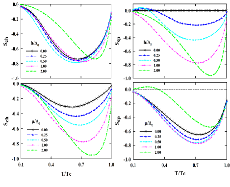
Figure 2: (Color online) The charge and spin thermopower of F-S junction as a function of temperature. The chemical potential is assumed to be $\mu=1.0\Delta_{0}$ in the top row and ferromagnetic exchange field values are $h=\left({0.0,0.25,0.5,1.0,2.0}\right)\Delta_{0}$. In the down panels, the applied magnetic exchange field is $h=1.0$ and the chemical potential values are $\mu=\left({0.0,0.25,0.5,1.0,2.0}\right)\Delta_{0}$. The temperature gradient is $T=0.1T_{c}$.

The corresponding wave functions of the above eigenvalues are

$$\begin{array}[]{l}\psi^{\text{F},\pm}_{e,\uparrow}(x)=\left(\mathbf{0^{2}},1,\pm e^{\pm i\alpha_{\uparrow}^{e}},\mathbf{0^{4}}\right)^{\bf T}e^{\pm ik_{x,\uparrow}^{\text{F},e}x}\;,\\ \psi^{\text{F},\pm}_{e,\downarrow}(x)=\left(1,\pm e^{\pm i\alpha_{\downarrow}^{e}},\mathbf{0^{2}},\mathbf{0^{4}}\right)^{\bf T}e^{\pm ik_{x,\downarrow}^{\text{F},e}x}\;,\\ \psi^{\text{F},\pm}_{h,\uparrow}(x)=\left(\mathbf{0^{4}},1,\mp e^{\pm i\alpha_{\uparrow}^{h}},\mathbf{0^{2}}\right)^{\bf T}e^{\pm ik_{x,\uparrow}^{\text{F},h}x}\;,\\ \psi^{\text{F},\pm}_{h,\downarrow}(x)=\left(\mathbf{0^{4}},\mathbf{0^{2}},1,\mp e^{\pm i\alpha_{\downarrow}^{h}}\right)^{\bf T}e^{\pm ik_{x,\downarrow}^{\text{F},h}x}\;,\end{array}$$ (13)

where $\mathbf{T}$ is a transpose operator and $\mathbf{0}^{n}$ denotes a $1\times n$ matrix with zero entries. From the conservation of the y-component wave vector ($k_{y}$) under the scattering processes, we factored out the corresponding multiplication i.e., $\exp(ik_{y}y)$. The $\alpha_{e,(h)}^{\uparrow(\downarrow)}$ variables are the propagation angles given by

$$\alpha_{\uparrow(\downarrow)}^{e(h)}=\arctan\left(\frac{q_{n}}{k_{x,\uparrow(\downarrow)}^{\text{F},e(h)}}\right)\;.$$ (14)

We denote $k_{y}\equiv q_{n}$ that can vary in interval $-\infty\leq q_{n}\leq+\infty$. The $e(h)$ superscript demonstrates the electron (hole)-like carriers and $\uparrow(\downarrow)$ subscript refers to the spin direction.

The superconductor region is assumed to be of s-wave symmetry type with step-like superconducting gap as,

$$\Delta(x,T)=\begin{cases}0&x\leq 0\\ \Delta(T)e^{i\phi}&x\geq 0\end{cases},$$ (15)

where $\phi$ is the macroscopic phase of the superconductor. The temperature-dependent gap of superconductor, $\Delta(T)=\Delta_{0}\tanh(1.76\sqrt{(T_{c}/T)-1})$, deduced from the BCS theory Ketterson1999 in which $\Delta_{0}$ is the superconductor gap at zero temperature. In superconducting region, $U_{0}$ denotes the electrostatic potential that is very large ($U_{0}\gg 1$) in actual experiments compared to other system energy scales to satisfy the mean field requirements Beenakker2006 . We diagonalize the corresponding Hamiltonian and obtain the eigenvalues of S region as,

$$\varepsilon=\sqrt{|\Delta_{0}|^{2}+\Big{(}\mu^{\text{S}}+U_{0}\pm\sqrt{(k_{x}^{\text{S}})^{2}+(k_{y})^{2}}\Big{)}^{2}}\;.$$ (16)

The associated wave functions are

$$\begin{array}[]{l}\psi^{\text{S},\pm}_{e,\kappa=1}(x)=\Big{(}e^{+i\beta},\pm e^{+i\beta},\mathbf{0^{2}},e^{-i\phi},\pm e^{-i\phi},\mathbf{0^{2}}\Big{)}^{\bf T}e^{\pm ik_{x}^{\text{S},e}x}\;,\\ \psi^{\text{S},\pm}_{e,\kappa=2}(x)=\Big{(}\mathbf{0^{2}},e^{+i\beta},\pm e^{+i\beta},\mathbf{0^{2}},e^{-i\phi},\pm e^{-i\phi}\Big{)}^{\bf T}e^{\pm ik_{x}^{\text{S},e}x}\;,\\ \psi^{\text{S},\pm}_{h,\kappa=1}(x)=\Big{(}e^{-i\beta},\mp e^{-i\beta},\mathbf{0^{2}},e^{-i\phi},\mp e^{-i\phi},\mathbf{0^{2}}\Big{)}^{\bf T}e^{\pm ik_{x}^{\text{S},h}x}\;,\\ \psi^{\text{S},\pm}_{h,\kappa=2}(x)=\Big{(}\mathbf{0^{2}},e^{-i\beta},\mp e^{-i\beta},\mathbf{0^{2}},e^{-i\phi},\mp e^{-i\phi}\Big{)}^{\bf T}e^{\pm ik_{x}^{\text{S},h}x}\;.\end{array}$$ (17)

The parameter $\beta$ is responsible for electron-hole conversions at F-S interface that depends on the temperature-dependent superconducting gap:

$$\beta=\begin{cases}+\leavevmode\nobreak\ \arccos(\varepsilon/\Delta)&\varepsilon\leq\Delta\\ -i\leavevmode\nobreak\ \text{arccosh}(\varepsilon/\Delta)&\varepsilon\geq\Delta\end{cases}.$$ (18)

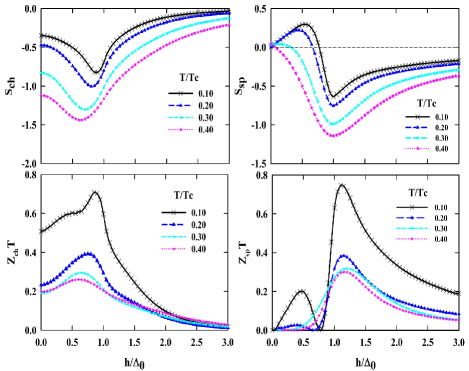
Figure 3: (Color online) The charge and spin thermopower and figures of merit of F-S junction as a function of the magnetic exchange field. The applied chemical potential is considered $\mu=1.0\Delta_{0}$ and the temperature gradient values are $T=\left(0.1,0.2,0.3,0.4\right)T_{c}$.

We normalize energies by the superconductor gap at zero temperature $\Delta_{0}$ and lengths by the superconducting coherent length $\xi_{S}=\hbar v_{F}/\Delta_{0}$.

In the F region, we assume that a right moving electron with $\uparrow$-spin direction hits the interface of F-S. We match the obtained wave-functions at the boundary $x=0$, and calculate the charge and thermal transmissions through normal and Andreev reflections at the interface from following equations:

$$\begin{array}[]{cc}r_{N\uparrow\downarrow}=\dfrac{-\cos\beta\sin(\alpha^{h}_{\downarrow}+\alpha^{e}_{\uparrow})/2+i\sin\beta\cos(\alpha^{h}_{\downarrow}-\alpha^{e}_{\uparrow})/2}{\cos\beta\cos(\alpha^{h}_{\downarrow}-\alpha^{e}_{\uparrow})/2+i\sin\beta\cos(\alpha^{h}_{\downarrow}+\alpha^{e}_{\uparrow})/2}\;,\\ \\ r_{A\uparrow\downarrow}=\dfrac{e^{-i\phi}\sqrt{\cos\alpha^{e}_{\uparrow}\cos\alpha^{h}_{\downarrow}}}{\cos\beta\cos(\alpha^{h}_{\downarrow}-\alpha^{e}_{\uparrow})/2+i\sin\beta\cos(\alpha^{h}_{\downarrow}+\alpha^{e}_{\uparrow})/2}\;.\end{array}$$ (19)

The thermoelectric properties of the junction are obtained using these equations. In the top row of Fig. 2, we demonstrate the temperature dependent charge and spin-dependent Seebeck coefficients ($S_{ch},S_{s}$) for different values of normalized magnetic exchange field ($h/\Delta_{0}$).

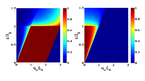
Figure 4: (Color online) The probability of normal $|r_{N}^{\uparrow}|^{2}$ (left) and Andreev $|r_{A}^{\downarrow}|^{2}$(right) reflections of F-S in low-doping regime with $\mu=h=1.0\Delta_{0}$ in which the conventional normal reflection is dominate. The temperature is $T=0.1T_{c}$.

We know from the previous calculations Rameshti2015 ; Ghosh2015 that in the magnetic graphene, the strong thermoelectric effects happened in the intermediate temperatures when the $k_{B}T$ parameter is in the order of $\mu+h$. In the superconductor graphene-based junction, we have two separate regimes: i) Weak field regime with $h\leq\Delta_{0}$ in which charge and spin-dependent Seebeck coefficients have a non-linear relation with temperature gradient and increase with increasing $h$. This fact is the consequence of the existence of ferromagnetic exchange potential. It is not only leads to an imbalance between the population of $\uparrow$- and $\downarrow$- spins in graphene sheet, but also can affect the amplitudes of Andreev reflections. However, in this regime the graphene is doped ($\mu\neq 0$)and both spin and charge currents exist while the second dominates. For $h\leq\mu$, increasing Andreev reflections leads to a non-linear increase in thermoelectric effects. ii) $h\geq\Delta_{0}$ in which increasing the chemical potential at higher temperatures leads to decreasing the spin thermopower and enhancing the charge thermopower. Since in graphene-based systems the doping can be controlled easily, one can reach the regimes in which the Fermi energy is comparable to thermal energy $k_{B}T$ to have a more efficient values of Seebeck coefficients (See the bottom row of Fig. 2). Moreover, at very low temperatures, $T/T_{c}\ll\Delta_{0}$, the values of charge and spin-dependent Seebeck coefficients are very small and go to zero with respect to the temperature.

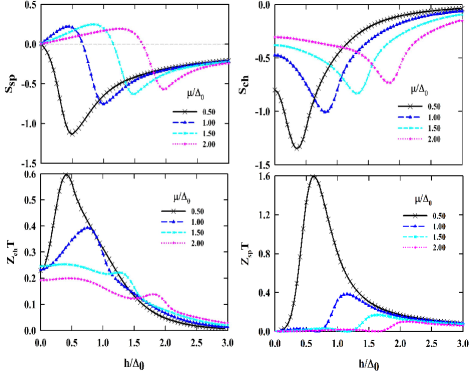
Figure 5: (Color online) The charge and spin-dependent Seebeck and figures of merit of F-S junction as a function of normalized magnetic exchange field. The chemical potential values are $\mu=\left(0.5,1.0,1.5,2.0\right)\Delta_{0}$ and the temperature is equal to $0.1T_{c}$.

In our subsequence analysis we study the dependence of the thermoelectric coefficients on the value of magnetic exchange field in Fig. 3. For some small values of $h$ and low enough temperature, the spin-dependent Seebeck effect has positive value while the charge Seebeck effect becomes all negative. We know from the dispersion relation of ferromagnetic graphene that in the low-doping regime ($\mu\leq\Delta_{0}$), the $\uparrow$-spin electrons and $\downarrow$-spin holes in the conduction and valance bands of graphene accompany each other to build the spin-dependent Seebeck effect. At low magnetic exchange field, the temperature gradient caused carriers with different spin directions to compete with each other resulting in an spin accumulation. For better analysis, the probabilities of normal ($|r_{N}^{\uparrow}|^{2}$) and Andreev $(|r_{A}^{\downarrow}|^{2})$ reflections are shown in Fig. 4. It can be easily conclude that the $\uparrow$-spin carriers dominate the spin-dependent Seebeck coefficient and since they carry negative current, the $S_{s}$ is negative, regardless to the strength of spin-splitting (Fig. 4). In low-temperature regime ($T/T_{c}\leq 0.2$) there is a sign change in the spin thermopower. But at higher temperatures, the spin-dependent Seebeck coefficient becomes all negative dominated by majority $\uparrow$-spin carriers.

Experimentally, by tunning the chemical potential, the charge carriers of graphene can be easily controlled. Consequently, the Fermi level in graphene can be electron-like or hole-like. Moreover, the magnetic exchange field in ferromagnetic region also changed the Fermi level of carriers. We use this fact for controlling the sign of spin-dependent thermopower of the junction, as shown in Fig. 5. In low-doped regime, the amplitude of the charge (spin) Seebeck coefficients and figures of merit is large because the thermal transport is very weak but the thermoelectric effect is not. These coefficients also vary by changing the gate voltages due to the changing in the transmission probabilities. As it is expected, the maximum values of spin (charge) figure of merit occurs at some $h$ above (below) the value of $\mu$.

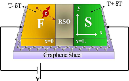
Figure 6: Schematic illustration of a graphene-based F-RSO-S junction. Similar to Fig.1, the junction is set in the x-y plane and a possible path of an incident spin-up electron at the F-RSO interface is also shown in the F region. The boundaries are considered at $x=0$ and $x=L$.

III.2 F-RSO-S Junction

It is known that the imposition of the thermal gradient implies an equilibrium between electrons and their counterparts. This effect along with ferromagnetic features produce spin thermopower in the junction, as discussed in the previous section. Now, we set the spin-mixer barrier with length of L in the middle of ferromagnetic and superconductor regions of graphene as shown in Fig. 6. The importance of this suggestion is that the spin-mixing phases in the proximity-induced RSO region provides singlet to triplet conversion Beiranvand2016 in the heterostructure gives rise to an spin transport mechanism through ferromagnetic region with strong exchange splitting of its bands. In this case, the Hamiltonian $H$, in Eq. 11 consists of two parts named $\mathcal{H}_{D}$ and $\mathcal{H}_{\text{RSO}}=-\lambda\left(s_{y}\otimes\sigma_{x}-s_{x}\otimes\sigma_{y}\right)$ in which $\lambda$ is the Rashba spin-orbit parameter. By diagonalizing the Hamiltonian of RSO region, we find the following dispersion relation:

$$\begin{array}[]{cc}\varepsilon=\pm\mu^{\text{RSO}}+\zeta\sqrt{(k_{x}^{\text{RSO}})^{2}+(k_{y})^{2}+\lambda^{2}}+\eta\lambda\;,\end{array}$$ (20)

where $\eta,\zeta=\pm 1$ indicate band indices. In contrast to intrinsic spin orbit couplings, the energy spectrum in the presence of RSO is gap-less with a splitting of magnitude $2\lambda$ between sub-bands. This sub-band splitting results in interesting phenomena Beiranvand2016 . The wave-functions associated with the eigenvalues can be expressed by:

$$\begin{array}[]{l}\psi^{\text{RSO},\pm}_{e,\eta=+1}(x)=\Big{(}\mp if_{+}^{e}e^{\mp i\theta_{+}^{e}},-i,1,\pm f_{+}^{e}e^{\pm i\theta_{+}^{e}},\mathbf{0^{4}}\Big{)}^{\bf T}e^{\pm ik_{x+}^{e}x}\;,\\ \psi^{\text{RSO},\pm}_{e,\eta=-1}(x=\Big{(}\pm f_{-}^{e}e^{\mp i\theta_{-}^{e}},1,-i,\mp if_{-}^{e}e^{\pm i\theta_{-}^{e}},\mathbf{0^{4}}\Big{)}^{\bf T}e^{\pm ik_{x-}^{e}x}\;,\\ \psi^{\text{RSO},\pm}_{h,\eta=+1}(x)=\Big{(}\mathbf{0^{4}},\mp if_{+}^{h}e^{\mp i\theta_{+}^{h}},-i,1,\pm f_{+}^{h}e^{\pm i\theta_{+}^{h}}\Big{)}^{\bf T}e^{\pm ik_{x+}^{h}x}\;,\\ \psi^{\text{RSO},\pm}_{h,\eta=-1}(x)=\Big{(}\mathbf{0^{4}},\pm f_{-}^{h}e^{\mp i\theta_{-}^{h}},1,-i,\mp if_{-}^{h}e^{\pm i\theta_{-}^{h}}\Big{)}^{\bf T}e^{\pm ik_{x-}^{h}x}\;.\end{array}$$ (21)

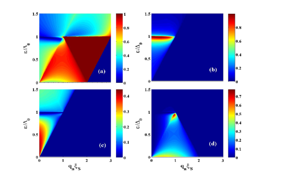
Figure 7: (Color online) Back scattering probabilities of an incident $\uparrow$-spin particle at $x=0$ as a function of applied voltage $\varepsilon/\Delta_{0}$ across the junction and the transverse momentum $q_{n}\xi_{S}$ for (a) conventional normal reflection $|r_{N}^{\uparrow}|^{2}$, (b) conventional Andreev reflection $|r_{A}^{\downarrow}|^{2}$, (c) spin-flipped normal reflection $|r_{N}^{\downarrow}|^{2}$, and (d) anomalous Andreev reflection $|r_{A}^{\uparrow}|^{2}$. The input values are $\mu=h=1.0\Delta_{0}$, $T=0.1T_{c}$ and $\lambda=5.0\Delta_{0}$.

Similar to the F and S region, each wave functions in the RSO region must be multiplied to $e^{iq_{n}y}$, where omitted here because of simplicity.

The definition of auxiliary parameters are:

$$\begin{array}[]{cc}f_{\eta}^{e}=\sqrt{1+2\eta\lambda(\mu^{\text{RSO}}+\varepsilon)^{-1}}\;,\\ f_{\eta}^{h}=\sqrt{1+2\eta\lambda(\mu^{\text{RSO}}-\varepsilon)^{-1}}\;,\end{array}$$ (22)

and

$$\begin{array}[]{cc}\theta_{\eta}^{e}=\arctan\left(q_{n}/k_{x,\eta}^{e}\right)\;,\\ \theta_{\eta}^{h}=\arctan\left(q_{n}/k_{x,\eta}^{h}\right)\;,\end{array}$$ (23)

where $\theta_{\eta}^{e}$ and $\theta_{\eta}^{h}$ are the electron and hole propagation angles in the region with spin-orbit interaction. We note that if the transverse component of wave-vector goes beyond a critical value $q^{c}$, the wave-functions turn to evanescent modes. Here, however, since the RSO region is confined between F and S regions, the evanescent modes contribute to the quantum transport process. We thus take both the propagating and decaying modes into account throughout our calculations. By matching the wavefunctions at the interfaces, i.e., $\Psi^{\text{F}}(x)=\Psi^{\text{RSO}}(x)$ at $x=0$ and $\Psi^{\text{RSO}}(x)=\Psi^{\text{S}}(x)$ at $x=L$, we obtain all of the scattering coefficients Beiranvand2016 .

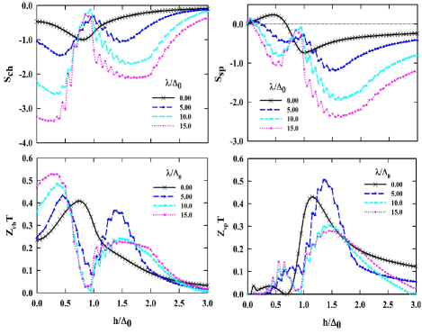
Figure 8: (Color online) The charge and spin-dependent Seebeck coefficients and figures of merit of F-RSO-S junction as a function of normalized $h$. $T=0.1T_{c}$ and $\mu=1.0\Delta_{0}$.

In this case, the transmission probabilities have more complicated energy-dependent form. So, the results could not report analytically. Consider, for instance, the four scattering processes of an incident $\uparrow$-spin electron arriving at the RSO interface from the ferromagnetic side. For $\lambda=0$, the intermediate region acts like a normal graphene. But, at nonzero values of $\lambda$, it can undergo an spin-mixing process in the RSO segment. For $\varepsilon\leq\Delta$, the incident particle cannot penetrate deep into the superconductor and gets reflected back into the ferromagnetic region either in the form of an electron (specular reflection) or, alternatively, as a hole (Andreev reflection). In this case, in addition to the normal reflection $(r_{N}^{\uparrow})$ and the conventional Andreev reflection $(r_{A}^{\downarrow})$, the probabilities of anomalous Andreev reflection ($r_{A}^{\uparrow}$) and unconventional normal reflection ($r_{N}^{\downarrow}$) have finite amplitudes Beiranvand2016 . If $\lambda$ is chosen properly, one can be able to reach an approximately high value of thermopower coefficients through applying spin-orbit interaction in the system.

The numerically obtained results for conventional and anomalous normal and Andreev reflections are presented in Fig. 7 in four different panels. It should be noted that, in order to achieve a high value of spin-dependent Seebeck coefficient with the possibility of using in the spin-thermoelectric devices, the length of suggested system should be in the order of 1 $\mu m$ Guimaraes2014 . Since the device length is normalized to the superconducting coherence length ($\xi_{S}$), all of our supposed structures are easily applicable in current experimental setups. Furthermore, in graphene, the Rashba spin-orbit coupling is in the order of $\approx$ 17 meV and the typical superconducting gap is about $0.1-3$ meV. So, in the theoretical point of view, we can easily increasing the RSO parameter ($\lambda$) up to 15 times greater than the value of $\Delta_{0}$ and the results can be experimentally reliable.

Since the Rashba spin-orbit interaction provides a spin mixing procedure in the middle region, one can find appropriate amounts of $\mu$, $h$ and $\lambda$ in which the charge and spin currents reach to their critical values. In Fig. 8, the numerically obtained results for charge and spin-dependent Seebeck coefficients are presented as a function of $h$. In this figure, we show the possibility of enhancing the spin-dependent thermopower in graphene devices by spin-orbit engineering to a large value of 2.5$k_{B}e$. The maximum value of the spin thermopower ($S^{max}_{s}$) was shown to increase with increasing the Rashba parameter. Remarkably, with a magnetic exchange field of $h\approx 0.1\Delta_{0}$, the charge Seebeck coefficient can also reach a value greater than 3.0$k_{B}e$, which is approximately 15 times larger than the value in pristine graphene.

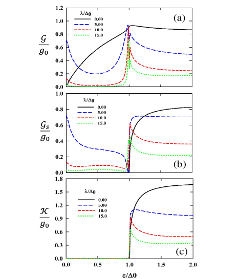
Figure 9: (Color online) The normalized (a) charge, (b) spin and (c) thermal conductances versus normalized energy. $T=0.1T_{c}$ and $\mu=h=1.0\Delta_{0}$.

Furthermore, we observe a critical zero point in which both charge and spin Seebeck effects drop down to zero. The origin of this effect in the low-doped regime can be understood from transmission coefficients. In this regime ($\mu\approx\Delta_{0}$), when the RSO parameter is zero ($\lambda=0$), we have normal region with finite width instead of RSO region which is the origin of resonant tunneling. In this case, there are only two reflection probabilities for a $\uparrow$-spin electron hitting the interface: ($a$) conventional normal reflection ($r_{N}^{\uparrow}$) and ($b$) retro Andreev reflection ($\varepsilon\leq\Delta_{0}$) or specular Andreev reflection ($\varepsilon\geq\Delta_{0}$), depending on the quasi-particle’s energy. Tuning the system parameters, ($\mu\approx\Delta_{0}$), $\lambda\neq 0$ lead to spin-mixing process in the RSO segment. This effect is responsible to tiny oscillations in the charge and spin-dependent Seebeck curves (See Fig. 8). This spin mixing process will increase the amplitudes of resonant oscillations. In addition, the transmission probability spectrum drops to zero for energy corresponding to the Fermi level position which are known as specular AR limit. In this case, the conventional Andreev reflected hole is placed in the valence with a specular reflection process whereas the anomalous one passes through the conduction band with a retro-reflected process. Thus, the reflected holes separate from each other with respect to their spin directions Beiranvand2016 . This suggests that there is a potential for application of this setup for cooling in the spin-dependent apparatuses.

Another experimentally measurable quantity in our supposed systems is the conductance of the junction. The behavior of charge, spin and thermal conductances are shown in Fig. 9. The presence of exchange energy $h$ in the F region results in an imbalance between carriers. In the presence of RSO coupling $\lambda\neq 0$, however, due to the possibility of spin-mixing in this region, the spin-polarized conductance can be also nonzero in the sub-gap region $\varepsilon\leq\Delta_{0}$. The enhancement of sub-gap spin conductance also traces back to the generation of equal-spin triplet correlations as discussed previously Beiranvand2016 . It is obvious from Eq. (20) that further increase in the value of RSO parameter leads to large band splitting between the $\eta=1$ and $\eta=-1$ bands in the RSO region. Owing to this effect contribution of $\eta=1$ band in transport mechanism is negligible and leads to reduction of the values of the spin, charge and thermal conductances of the junction.

IV Conclusion

To conclude, we have developed a theoretical framework to study the thermal transport properties of ferromagnetic-superconductor (F-S) and ferromagnetic-Rashba spin-orbit-superconductor (F-RSO-S) junctions by calculating charge and spin-dependent thermopower of the junctions. Our results demonstrate that the simultaneous effect of spin-splitting field and spin orbit coupling leads to a strong suppression of the spin imbalances which can affect on the usually small thermoelectric coefficients in superconducting nanostructures. The results show that in the low-doped regime, by engineering the spin-orbit interaction, the charge and spin thermopowers can reach to their maximums up to 3.0$k_{B}/e$ and 2.5$k_{B}/e$, respectively in the F-RSO-S junction. Remarkably, these coefficients have a zero-point critical value with respect to magnetic exchange field and chemical potential. This effect disappears when the Rashba coupling is absent. These results suggest that graphene-based superconductors can be used in spin-caloritronic devices.

V Acknowledgment

The authors acknowledge the Iran national science foundation (INSF) for financial support.

References

- (1) K. S. Novoselov, A. K. Geim, S. V. Morozov, D. Jiang, Y. Zhang, S. V. Dubonos, I. V. Grigorieva, and A. A. Firsov, Electric Field Effect in Atomically Thin Carbon Films, Science 306, 666 (2004).
- (2) K. S. Novoselov, A. K. Geim, S. V. Morozov, D. Jiang, M. I. Katsnelson, I. V. Grigorieva, S. V. Dubonos, and A. A. Firsov, Two-dimensional gas of massless Dirac fermions in graphene, Nature 438, 197 (2005).
- (3) A. De Martino, L. DellÁnna, and R. Egger, Magnetic Confinement of Massless Dirac Fermions in Graphene, Phys. Rev. Lett. 98, 066802 (2007).
- (4) C. Park, L. Yang, Y. Son, M. L. Cohen, and S. G. Louie, Anisotropic behaviors of massless Dirac fermions in graphene under periodic potentials, Nat. Phys. 4, 213 (2008).
- (5) A. H. Castro Neto, F. Guinea, N. M. R. Peres, K. S. Novoselov, and A. K. Geim, The electronic properties of graphene, Rev. Mod. Phys. 81, 109 (2009) .
- (6) F. Bonaccorso, Z. Sun, T. Hasan, and A. C. Ferrari, Graphene photonics and optoelectronics, Nat. Pho. 4, 611 (2010).
- (7) P. Avouris, Graphene: Electronic and Photonic Properties and Devices, Nano. Lett. 10 4285 (2010).
- (8) Q. Bao, and K. P. Loh, Graphene Photonics, Plasmonics, and Broadband Optoelectronic Devices, ACS Nano, 6, 3677 (2012).
- (9) A. G. Moghaddam, and M. Zareyan, Graphene-Based Electronic Spin Lenses, Phys. Rev. Lett. 105, 146803 (2010).
- (10) D. Pesin, and A. H. MacDonald, Spintronics and pseudospintronics in graphene and topological insulators, Nat. Mat. 11, 409 (2012).
- (11) W. Han,R. K. Kawakami, M. Gmitra, and J. Fabian, Graphene spintronics, Nat. Nanotech. 9, 807 (2014).
- (12) B. Ghosh, Spin transport in bilayer graphene, J. App. Phys. 109 013706 (2011).
- (13) Y. Zhang, Y. -W. Tan, H. L. Stormer, and P. Kim, Experimental observation of the quantum Hall effect and Berry’s phase in graphene, Nat. 438, 201 (2005).
- (14) K. S. Novoselov, Z. Jiang, Y. Zhang, S. V. Morozov, H. L. Stormer, U. Zeitler, J. C. Maan, G. S. Boebinger, P. Kim, and A. K. Geim, Room-Temperature Quantum Hall Effect in Graphene, Science, 315, 1379(2007).
- (15) V. P. Gusynin, and S. G. Sharapov, Unconventional Integer Quantum Hall Effect in Graphene, Phys. Rev. Lett. 95, 146801 (2005).
- (16) P. Rickhaus, M. Weiss, L. Marot, and Ch. Schönenberger, Quantum Hall Effect in Graphene with Superconducting Electrodes, Nano. Lett. 12, 1942 (2012) .
- (17) M. I. Katsnelson, K. S. Novoselov, and A. K. Geim, Chiral tunnelling and the Klein paradox in graphene, Nat. Phys. 2, 620 (2006) .
- (18) C. W. J. Beenakker, Colloquium: Andreev reflection and Klein tunneling in graphene, Rev. Mod. Phys. 80, 1337 (2008).
- (19) M. Zareyan, H. Mohammadpour, and A. G. Moghaddam, Andreev-Klein reflection in graphene ferromagnet-superconductor junctions, Phys. Rev. B 78, 193406 (2008).
- (20) C. E. Malec, D. Davidović, Transport in graphene tunnel junctions, J. App. Phys. 109 064507 (2011).
- (21) A. I. Buzdin, Proximity effects in superconductor-ferromagnet heterostructures, Rev. Mod. Phys. 77, 935 (2005).
- (22) H. B. Heersche, P. Jarillo-Herrero, J. B. Oostinga, L. M. K. Vandersypen, and A. F. Morpurgo, Sol. Sta. Comm. 143, 72 (2007).
- (23) Z. Wang, C. Tang, R. Sachs, Y. Barlas, and J. Shi, Proximity-Induced Ferromagnetism in Graphene Revealed by the Anomalous Hall Effect, Phys. Rev. Lett. 114, 016603 (2015)
- (24) G. E. Blonder, M. Tinkham, and T. M. Klapwijk, Transition from metallic to tunneling regimes in superconducting microconstrictions: Excess current, charge imbalance, and supercurrent conversion, Phys. Rev. B. 25, 4515 (1982) .
- (25) B. Z. Rameshti, and A. G. Moghaddam, Spin-dependent Seebeck effect and spin caloritronics in magnetic graphene, Phys. Rev. B. 91, 155407 (2015).
- (26) A. Ghosh, H.O. Frota, Spin caloritronics in graphene, J. App. Phys. 117, 223907 (2015).
- (27) M. Inglot, V. K. Dugaev, and J. Barnaś, Thermoelectric and thermospin transport in a ballistic junction of graphene, Phys. Rev. B. 92, 085418 (2015).
- (28) D. Dragoman, and M. Dragoman, Giant thermoelectric effect in graphene, Appl. Phys. Lett. 91, 203116 (2007).
- (29) X. Xu, N. M. Gabor, J. S. Alden, A. M. van der Zande, and P. L. McEuen, Photo-Thermoelectric Effect at a Graphene Interface Junction, Nano Lett. 10, 562 (2010).
- (30) M. Salehi, M. Alidoust, Y. Rahnavard, and G. Rashedi, Thermal transport properties of graphene-based ferromagnetic/singlet superconductor/ferromagnetic junctions, J. Appl. Phys. 107, 123916 (2010).
- (31) M. Salehi, M. Alidoust, and G. Rashedi, Signatures of d-Wave Symmetry on Thermal Dirac Fermions in Graphene-Based F/I/d Junctions, J. Appl. Phys. 108, 083917 (2010).
- (32) K. Uchida, S. Takahashi, K. Harii, J. Ieda, W. Koshibae, K. Ando, S. Maekawa, and E. Saitoh, Observation of the spin Seebeck effect,Nature 455, 778 (2008) .
- (33) C. M. Jaworski, R. C. Myers, E. Johnston-Halperin, and J. P. Heremans, Giant spin Seebeck effect in a non-magnetic material, Nature 487, 210 (2012).
- (34) Y. M. Zuev, W. Chang, and P. Kim, Thermoelectric and Magnetothermoelectric Transport Measurements of Graphene,Phys. Rev. Lett. 102, 096807 (2009).
- (35) P. Wei, W. Bao, Y. Pu, C. N. Lau, and J. Shi, Anomalous Thermoelectric Transport of Dirac Particles in Graphene,Phys. Rev. Lett. 102, 166808 (2009) .
- (36) A. Ozaeta, P. Virtanen, F. S. Bergeret, and T. T. Heikkilä, Predicted Very Large Thermoelectric Effect in Ferromagnet-Superconductor Junctions in the Presence of a Spin-Splitting Magnetic Field, Phys. Rev. Lett. 112, 057001 (2014).
- (37) E. I. Rashba, Graphene with structure-induced spin-orbit coupling: Spin-polarized states, spin zero modes, and quantum Hall effect, Phys. Rev. B 79, 161409(R) (2009) .
- (38) C. L. Kane and E. J. Mele, Quantum Spin Hall Effect in Graphene, Phys. Rev. Lett. 95, 226801(2005).
- (39) R. Beiranvand, H. Hamzehpour, and M. Alidoust, Tunable anomalous Andreev reflection and triplet pairings in spin-orbit-coupled graphene, Phys. Rev. B. 94, 125415 (2016).
- (40) A. Avsar, J. Y. Tan, T. Taychatanapat, J. Balakrishnan, G. K. W. Koon, Y. Yeo, J. Lahiri, A. Carvalho, A. S. Rodin, E. C. T. O’Farrell, G. Eda, A. H. Castro Neto, and B. Ozyilmaz, Spin–orbit proximity effect in graphene, Nat. Commun., 5, 4875 (2014).
- (41) H. Min, J. E. Hill, N. A. Sinitsyn, B. R. Sahu, L. Kleinman, and A. H. MacDonald, Intrinsic and Rashba spin-orbit interactions in graphene sheets, Phys. Rev. B 74 165310 (2006).
- (42) D. Huertas-Hernando, F. Guinea, and A. Brataas, Spin-orbit coupling in curved graphene, fullerenes, nanotubes, and nanotube caps, Phys. Rev. B. 74 155426 (2006).
- (43) Y. Yao, F. Ye, X. L. Qi, S. -C. Zhang, and Z. Fang, Spin-orbit gap of graphene: First-principles calculations, Phys. Rev. B. 75 041401(R)(2007).
- (44) C. López-Monís, A. Matos-Abiague, and J. Fabian, Tunneling anisotropic thermopower and Seebeck effects in magnetic tunnel junctions, Phys. Rev. B. 90, 174426 (2014).
- (45) M. I. Alomar, L. Serra, and D. Sánchez, Seebeck effects in two-dimensional spin transistors, Phys. Rev. B. 91, 075418 (2015).
- (46) K. Uchida, J. Xiao, H. Adachi, J. Ohe, S. Takahashi, J. Ieda, T. Ota, Y. Kajiwara, H. Umezawa, H. Kawai, G. E. W. Bauer, S. Maekawa, and E. Saitoh, Spin Seebeck insulator, Nat. Mat. 9, 894 (2010).
- (47) K. Uchida, H. Adachi, T. Ota, H. Nakayama, S. Maekawa, and E. Saitoh, Observation of longitudinal spin-Seebeck effect in magnetic insulators,Appl. Phys. Lett. 97, 172505 (2010).
- (48) D. Qu, S. Y. Huang, J. Hu, R. Wu, and C. L. Chien, Intrinsic Spin Seebeck Effect in Au/YIG, Phys. Rev. Lett. 110, 067206 (2013).
- (49) F. Hübler, M. J. Wolf, D. Beckmann, and H. v. Löhneysen, Long-Range Spin-Polarized Quasiparticle Transport in Mesoscopic Al Superconductors with a Zeeman Splitting,Phys. Rev. Lett. 109, 207001 (2012).
- (50) S. -Y. Hwang, R. López, and D. Sánchez, Large thermoelectric power and figure of merit in a ferromagnetic–quantum dot–superconducting device, Phys. Rev. B. 94, 054506 (2016).
- (51) S. Kolenda, M. J. Wolf, and D. Beckmann, Observation of Thermoelectric Currents in High-Field Superconductor-Ferromagnet Tunnel Junctions, Phys. Rev. Lett. 116, 097001 (2016).
- (52) M. Silaev, J. Garaud, and E. Babaev, Unconventional thermoelectric effect in superconductors that break time-reversal symmetry, Phys. Rev. B. 92, 174510 (2015).
- (53) T. Yokoyama, J. Linder, and A. Sudbø, Heat transport by Dirac fermions in normal/superconducting graphene junctions, Phys. Rev. B 77, 132503 (2008).
- (54) C. W. J. Beenakker, Specular Andreev Reflection in Graphene, Phys. Rev. Lett. 97, 067007 (2006).
- (55) P. G. de Gennes, Superconductivity in Metals and Alloys, Westview Press (1966).
- (56) K. Halterman, O. Valls, and M. Alidoust, Spin-Controlled Superconductivity and Tunable Triplet Correlations in Graphene Nanostructures, Phys. Rev. Lett. 111 046602 (2013).
- (57) J. B. Ketterson, and S. N. Song, Superconductivity, Cambridge University Press (1999).
- (58) M. H. D. Guimarães, J. J. van den Berg, I. J. Vera-Marun, P. J. Zomer, and B. J. van Wees, Spin transport in graphene nanostructures, Phys. Rev. B, 90, 235428 (2014).