Embedding cosmological inflation, axion dark matter and seesaw mechanism in a 3-3-1 gauge model

Abstract

The Peccei-Quinn symmetry is an automatic symmetry of the 3-3-1 gauge models which, consequently are not plagued with the strong CP problem. Nevertheless, the axion that emerges from spontaneous breaking of Peccei-Quinn symmetry cannot be made invisible in the original versions of these models, unless we extend their scalar sector by an additional neutral scalar singlet. In this case we show that if, we also add heavy neutrinos in the singlet form, we get to solve three interesting open questions at once: the real component of the neutral scalar singlet driving inflation, the axion playing the role of the dark matter of the universe and standard neutrinos gaining masses through seesaw mechanism.

I Introduction

The $SU(3)_{C}\times SU(3)_{L}\times U(1)_{N}$ (3-3-1) gauge models for the electroweak interactions are interesting in their own right. For example, in these models generations cannot replicate unrestrictedly as in the standard model (SM), since they are not exact replicas of one another and each is separately anomalous. However, when three generations are taken into account, gauge anomaly is automatically canceled Frampton (1992), providing a reason for the existence of three families of fermions.

Also, the set of constraints from gauge invariance of the Yukawa interactions together with those coming from the anomaly cancellation conditions are enough to fix the electric charges of the particles in the 3-3-1 model, thus providing an understanding of the pattern of electric charge quantization de Sousa Pires and Ravinez (1998)de Sousa Pires (1999).

In what concerns the Peccei-Quinn (PQ) symmetry, it is an automatic symmetry of these models, thus elegantly solving the strong CP-problem Pal (1995). However, the original versions of the 3-3-1 gauge models furnish an unrealistic axion because of its sizable couplings with the standard particles Weinberg (1978)Wilczek (1978). In order to we have an invisible axion a neutral scalar singlet must be added to the conventional scalar sector (three Higgs triplets) Kim (1979)Shifman et al. (1980)Dine et al. (1981).

Regarding neutrino masses, canonical seesaw mechanisms, as type I and type II, as well as the inverse seesaw mechanism are easily implemented in the framework of the 3-3-1 models Montero et al. (2002)Dias et al. (2012)Dong and Long (2008)Boucenna et al. (2015) .

Last in the sequence but not least in importance, we remember that some versions of the 3-3-1 models have in their conventional particle content a stable and neutral particle that may play the role of cold dark matter in the WIMP formde S. Pires and Rodrigues da Silva (2007)Mizukoshi et al. (2011)Rodrigues da Silva (2014)Dong et al. (2015). These are only a few remarkable things that make 3-3-1 models interesting candidates for new physics beyond the SM.

Although theoretical and phenomenological aspects of the 3-3-1 gauge models have received considerable attention, cosmological issues have been much less developed, in particular, the inflationary scenario was scarcely studied in a supersymmetric version of 3-3-1 model Huong and Long (2010); Long (2015). Thus, it would be very interesting if inflation could be implemented in the framework of other 3-3-1 gauge models, even without supersymmetry.

At this point we would like to remark that a possible way of providing a common origin to cosmological inflation, the cold dark mater, neutrino masses and solution to the strong CP-problem is by adding exotic vector like quarks, right-handed neutrinos and neutral scalar singlet to the standard model, building a scenario called SMASH Dias et al. (2014)Barenboim and Park (2016)Ballesteros et al. (2016a)Ballesteros et al. (2016b). This packet of new particles together with adequate interactions allows the implementation of the PQ symmetry in the standard models. The PQ symmetry is spontaneously broken when the neutral scalar singlet develop vacuum expectation value (VEV) different from zero. In this circumstance, the imaginary part of the neutral scalar singlet will be the invisible axion, which may play the role of dark matter, while the real part may play the role of the inflaton. Moreover, on coupling the neutral scalar to the right-handed neutrino, through an Yukawa interaction, the VEV of the neutral scalar, that is around $(10^{10}-10^{11})$ GeV, will generate heavy neutrinos that may trigger the type I seesaw mechanism yielding small neutrino masses for the standard neutrinos. The problem with this scenario is that it generates an inflaton potential of the type $\lambda\phi^{4}$ which is practically excluded by the current bounds from PLANCK15 Ade et al. (2016). A way of circumventing such a problem is considering that the inflaton couples non-minimally with the scalar curvature $R$ or taking into account radiative corrections to the inflaton potential. The question we follow here is that if it is possible to implement such a scenario into the 3-3-1 model framework, since PQ symmetry is an automatic symmetry of the model. In this paper we show that this is possible when radiative corrections are taken into account for the inflaton potential.

The paper is divided in the following way: In Sec. II we revisit the 3-3-1 model that contains an invisible axion in its spectrum. Next, in Sec. III, we develop the inflationary paradigm in such model. We finally conclude in Sec. IV.

II The 3-3-1 model, the Pecei-Quinn symmetry and the invisible axion

The model developed here is one proposed in Ref. Dias et al. (2003) which is a modification of the original one Singer et al. (1980)Montero et al. (1993)Foot et al. (1994). The first modification is in the leptonic sector where heavy right-handed neutrinos in the singlet form are added to the model,

$$f^{a}_{L}=\left(\begin{array}[]{c}\nu^{a}_{L}\\ e^{a}_{L}\\ (\nu^{c}_{R})^{a}\end{array}\right)\sim(1\,,\,3\,,\,-1/3)\,,\,\,\,e_{aR}\,\sim(1,1,-1)\,,\,\,\,N_{aR}\,\sim(1,1,0)$$ (4)

with $a=1,2,3$ representing the three known generations. We are indicating the transformation under 3-3-1 after the similarity sign, “$\sim$”.

The quark sector is kept intact with one generation of left-handed fields coming in the triplet fundamental representation of $SU(3)_{L}$ and the other two composing an anti-triplet representation with the content,

$$Q_{iL}=\left(\begin{array}[]{c}d_{iL}\\ -u_{iL}\\ d^{\prime}_{iL}\end{array}\right)\sim(3\,,\,\bar{3}\,,\,0)\,,\,\,\,Q_{3L}=\left(\begin{array}[]{c}u_{3L}\\ d_{3L}\\ u^{\prime}_{3L}\end{array}\right)\sim(3\,,\,3\,,\,1/3)\,,$$ (11)

and the right-handed fields,

$$u_{iR}\,\sim(3,1,2/3)\,,\,d_{iR}\,\sim(3,1,-1/3)\,,\,d^{\prime}_{iR}\,\sim(3,1,-1/3)$$

$$u_{3R}\,\sim(3,1,2/3)\,,\,d_{3R}\,\sim(3,1,-1/3)\,,\,u^{\prime}_{3R}\,\sim(3,1,2/3),$$ (12)

where $j=1,2$ represent different generations. The primed quarks are the exotic ones but with the usual electric charges.

In order to generate the masses for the gauge bosons and fermions, the model requires only three Higgs scalar triplets. For our proposal here we add a neutral scalar singlet to these triplets transforming in the following way by the 3-3-1 symmetry,

$$\chi=\left(\begin{array}[]{c}\chi^{0}\\ \chi^{-}\\ \chi^{\prime 0}\end{array}\right)\sim(1\,,\,3\,,\,-1/3)\,\,,\,\,\eta=\left(\begin{array}[]{c}\eta^{0}\\ \eta^{-}\\ \eta^{\prime 0}\end{array}\right)\sim(1\,,\,3\,,\,-1/3),$$ (19)

$$\rho=\left(\begin{array}[]{c}\rho^{+}\\ \rho^{0}\\ \rho^{\prime+}\end{array}\right)\sim(1\,,\,3\,,\,2/3)\,,\,\,\,\,\,\,\,\phi\sim(1,1,0).$$ (23)

Thus the particle content of the model is extended by the fields $N_{a_{R}}$ and $\phi$ .

In order to keep intact the physics results of the Ref. Dias et al. (2003), the Lagrangian of the model must be invariant by the following set of discrete symmetries $Z_{11}\otimes Z_{2}$ but now with $Z_{11}$ acting as

$$\phi\,\,\,\,\, \rightarrow \,\,\,\,\,\omega^{-1}_{1}\phi\,,\,\,\,\,\,\,\,\,\,\,\,\,\,\,\,\,\,\,\,\,\,\,\,\,\,f_{aL}\,\,\,\,\,\,\,\rightarrow\,\,\,\,\,\,\,\omega_{1}f_{aL}\,,$$

$$\rho\,\,\,\,\, \rightarrow \,\,\,\,\,\omega^{-1}_{2}\rho\,,\,\,\,\,\,\,\,\,\,\,\,\,\,\,\,\,\,\,\,\,\,\,\,\,\,d_{aR}\,\,\,\,\,\,\,\rightarrow\,\,\,\,\,\,\,\omega_{2}d_{aR}\,,$$

$$\chi\,\,\,\,\, \rightarrow \,\,\,\,\,\omega^{-3}_{3}\chi\,,\,\,\,\,\,\,\,\,\,\,\,\,\,\,\,\,\,\,\,\,\,\,u_{3R}^{\prime}\,\,\,\,\,\,\,\,\rightarrow\,\,\,\,\,\,\,\omega_{3}u_{3R}^{\prime}\,,$$

$$Q_{iL}\,\,\,\,\, \rightarrow \,\,\,\,\,\omega^{-1}_{4}Q_{iL}\,,\,\,\,\,\,\,\,\,\,\,\,\,\,\,\,\,\,\,\,d_{iR}^{\prime}\,\,\,\,\,\,\,\rightarrow\,\,\,\,\,\,\,\omega_{4}d_{iR}^{\prime}\,,$$

$$\eta\,\,\,\,\, \rightarrow \,\,\,\,\,\omega^{-1}_{5}\eta\,,\,\,\,\,\,\,\,\,\,\,\,\,\,\,\,\,\,\,\,\,\,\,\,\,\,u_{aR}\,\,\,\,\,\,\,\rightarrow\,\,\,\,\,\,\,\omega_{5}u_{aR}\,,$$

$$Q_{3L}\,\,\,\,\, \rightarrow \,\,\,\,\,\omega_{0}Q_{3L}\,,\,\,\,\,\,\,\,\,\,\,\,\,\,\,\,\,\,\,\,N_{R}\,\,\,\,\,\rightarrow\,\,\,\,\,\omega^{-1}_{5}N_{R}\,,$$

$$e_{aR}\,\,\,\,\,\,\, \rightarrow \,\,\,\,\,\,\,\omega_{3}e_{aR}\,,$$ (24)

where $\omega_{k}\equiv e^{2\pi i\frac{k}{11}}\,,\,\{k=0,\pm 1,...,\pm 5\}$.

The $Z_{2}$ symmetry must act as

$$(\rho\,,\chi\,,d_{R}^{\prime}\,,u_{3R}^{\prime}\,,u_{R}\,,d_{R}\,,e_{R})\,\,\,\,\rightarrow\,\,\,\,-(\rho\,,\chi\,,d_{R}^{\prime}\,,u_{3R}^{\prime}\,,u_{R}\,,d_{R}\,,e_{R})\,.$$ (25)

These discrete symmetries yield the following Yukawa couplings

$${\cal L}^{Y} =G_{1}\bar{Q}_{3L}u^{\prime}_{3R}\chi+G_{2}^{ij}\bar{Q}_{iL}d^{\prime}_{jR}\chi^{*}+G_{3}^{3a}\bar{Q}_{3L}u_{aR}\eta+G_{4}^{ia}\bar{Q}_{iL}d_{aR}\eta^{*}$$ (26)

$$+G_{5}^{3a}\bar{Q}_{3L}d_{aR}\rho+G_{6}^{ia}\bar{Q}_{iL}u_{aR}\rho^{*}+g_{ab}\bar{f}_{aL}e_{bR}\rho+h_{ab}\bar{f}_{aL}\eta N_{bR}+h^{\prime}_{ab}\phi\bar{N}^{C}_{aR}N_{bR}+\mbox{H.c.}.$$

The transformations displayed in Eqs. (24) and (25) are a little different from the original case Dias et al. (2003). The reason of the modification is to accommodate the last two terms in the Lagrangian above. These terms are crucial for our proposal, as we will see later.

The allowed renormalizable and gauge invariant potential for this model is exactly the same as in the original case, i.e,

$$V_{H} = \mu_{\phi}^{2}\phi^{2}+\mu_{\chi}^{2}\chi^{2}+\mu_{\eta}^{2}\eta^{2}+\mu_{\rho}^{2}\rho^{2}+\lambda_{1}\chi^{4}+\lambda_{2}\eta^{4}+\lambda_{3}\rho^{4}+\lambda_{4}(\chi^{\dagger}\chi)(\eta^{\dagger}\eta)+\lambda_{5}(\chi^{\dagger}\chi)(\rho^{\dagger}\rho)$$ (27)

$$+\lambda_{6}(\eta^{\dagger}\eta)(\rho^{\dagger}\rho)+\lambda_{7}(\chi^{\dagger}\eta)(\eta^{\dagger}\chi)+\lambda_{8}(\chi^{\dagger}\rho)(\rho^{\dagger}\chi)+\lambda_{9}(\eta^{\dagger}\rho)(\rho^{\dagger}\eta)+\lambda_{10}(\phi\phi^{*})^{2}$$

$$+\lambda_{11}(\phi\phi^{*})(\chi^{\dagger}\chi)+\lambda_{12}(\phi\phi^{*})(\rho^{\dagger}\rho)+\lambda_{13}(\phi\phi^{*})(\eta^{\dagger}\eta)+\lambda_{\phi}\epsilon^{ijk}\eta_{i}\rho_{j}\chi_{k}\phi+H.c\,,$$

Other tiny change arises in the definition of the PQ charges. In order to have chiral quarks under $U_{PQ}(1)$, we need the following transformation

$$u_{aL} \rightarrow e^{-i\alpha X_{u}}u_{aL}\,,\,\,\,\,u_{aR}\,\,\,\rightarrow\,\,\,e^{i\alpha X_{u}}u_{aR}\,,$$

$$u_{3L}^{\prime} \rightarrow e^{-i\alpha X_{u}^{\prime}}u_{3L}^{\prime}\,,\,\,\,\,u_{3R}^{\prime}\,\,\,\rightarrow\,\,\,e^{i\alpha X_{u}^{\prime}}u_{3R}^{\prime}\,,$$

$$d_{aL} \rightarrow e^{-i\alpha X_{d}}d_{aL}\,,\,\,\,\,d_{aR}\,\,\,\rightarrow\,\,\,e^{i\alpha X_{d}}d_{aR}\,,$$

$$d_{iL}^{\prime} \rightarrow e^{-i\alpha X_{d}^{\prime}}d_{iL}^{\prime}\,,\,\,\,\,\,\,d_{iR}^{\prime}\,\,\,\rightarrow\,\,\,e^{i\alpha X_{d}^{\prime}}d_{iR}^{\prime}\,.$$ (28)

For the leptons we can define their PQ charges by,

$$e_{aL} \rightarrow e^{i\alpha X_{e}}e_{aL}\,,\,\,\,\,e_{aR}\,\,\,\rightarrow\,\,\,e^{i\alpha X_{eR}}e_{aR}\,,\,\,\,N_{aL}\rightarrow e^{i\alpha X_{N}}N_{aL}$$

$$\nu_{aL} \rightarrow e^{i\alpha X_{\nu}}\nu_{aL}\,,\,\,\,\,\nu_{aR}\,\,\,\rightarrow\,\,\,e^{i\alpha X_{\nu R}}\nu_{aR}\,.$$ (29)

With these assignments and taking the Yukawa interactions in Eq. (26) into account, as well as the non-hermitean terms $\eta\rho\chi\phi$, we easily see that the PQ charges for the scalars are constrained and imply the following relations:

$$X_{d}=-X_{u}\,,\,\,\,\,X_{d^{\prime}}=-X_{u^{\prime}}\,,\,\,\,\,X_{\nu}=X_{eR}\,,\,\,\,\,X_{e}=X_{\nu R}\,.$$ (30)

We can make the further choice $X_{d}=X_{d^{\prime}}$, leading to

$$X_{d}=X_{d^{\prime}}=-X_{u}=-X_{u^{\prime}}=-X_{e}=X_{eR}=X_{\nu}=-X_{\nu R}=X_{N}\,,$$ (31)

implying that the PQ symmetry is chiral for the leptons too. The scalars transform as

$$\phi \rightarrow e^{-2i\alpha X_{d}}\phi\,,\,\,\,\,\,\,\,\,\,\,\,\,\,\,\eta^{0}\,\,\,\,\rightarrow\,\,\,e^{2i\alpha X_{d}}\eta^{0}$$

$$\eta^{-} \rightarrow \eta^{-}\,,\,\,\,\,\,\,\,\,\,\,\,\,\,\,\,\,\,\,\,\,\,\,\,\,\,\,\,\,\,\eta^{\prime 0}\,\,\,\rightarrow\,\,\,e^{2i\alpha X_{d}}\eta^{\prime 0}$$

$$\rho^{+} \rightarrow \rho^{+}\,,\,\,\,\,\,\,\,\,\,\,\,\,\,\,\,\,\,\,\,\,\,\,\,\,\,\,\,\,\,\,\rho^{0}\,\,\,\,\rightarrow\,\,\,e^{-2i\alpha X_{d}}\rho^{0}$$

$$\rho^{\prime+} \rightarrow \rho^{\prime+}\,,\,\,\,\,\,\,\,\,\,\,\,\,\,\,\,\,\,\,\,\,\,\,\,\,\,\,\,\,\,\chi^{0}\,\,\,\rightarrow\,\,\,e^{2i\alpha X_{d}}\chi^{0}$$

$$\chi^{-} \rightarrow \chi^{-}\,,\,\,\,\,\,\,\,\,\,\,\,\,\,\,\,\,\,\,\,\,\,\,\,\,\,\,\,\,\,\chi^{\prime 0}\,\,\,\rightarrow\,\,\,e^{2i\alpha X_{d}}\chi^{\prime 0}.$$

It is now clear that the entire Lagrangian of the model is $U_{PQ}(1)$ invariant, providing a natural solution to the strong-CP problem.

To accomplish our proposal, let us consider that only $\chi^{\prime 0}$, $\rho^{0}$, $\eta^{0}$ and $\phi$ develop VEV and expand such fields around them in the standard way,

$$\chi^{\prime 0} = \frac{1}{\sqrt{2}}(v_{\chi^{\prime}}+R_{\chi^{\prime}}+iI_{\chi^{\prime}})\,,\,\,\,\,\,\,\,\eta^{0}=\frac{1}{\sqrt{2}}(v_{\eta}+R_{\eta}+iI_{\eta})\,,$$

$$\rho^{0} = \frac{1}{\sqrt{2}}(v_{\rho}+R_{\rho}+iI_{\rho})\,,\,\,\,\,\,\,\,\,\,\,\,\,\,\,\,\phi=\frac{1}{\sqrt{2}}(v_{\phi}+R_{\phi}+iI_{\phi})\,.$$ (33)

With such expansion, we obtain the set of constraint equations that guarantee that the potential has a minimum

$$\mu^{2}_{\chi}+\lambda_{1}v^{2}_{\chi^{\prime}}+\frac{\lambda_{4}}{2}v^{2}_{\eta}+\frac{\lambda_{5}}{2}v^{2}_{\rho}+\frac{\lambda_{11}}{2}v_{\phi}^{2}+\frac{A}{v_{\chi^{\prime}}^{2}}=0,$$

$$\mu^{2}_{\eta}+\lambda_{2}v^{2}_{\eta}+\frac{\lambda_{4}}{2}v^{2}_{\chi^{\prime}}+\frac{\lambda_{6}}{2}v^{2}_{\rho}+\frac{\lambda_{13}}{2}v^{2}_{\phi}+\frac{A}{v_{\eta}^{2}}=0,$$

$$\mu^{2}_{\rho}+\lambda_{3}v^{2}_{\rho}+\frac{\lambda_{5}}{2}v^{2}_{\chi^{\prime}}+\frac{\lambda_{6}}{2}v^{2}_{\eta}+\frac{\lambda_{12}}{2}v^{2}_{\phi}+\frac{A}{v_{\rho}^{2}}=0,$$

$$\mu^{2}_{\phi}+\lambda_{10}v^{2}_{\phi}+\frac{\lambda_{11}}{2}v^{2}_{\chi^{\prime}}+\frac{\lambda_{12}}{2}v^{2}_{\rho}+\frac{\lambda_{13}}{2}v^{2}_{\eta}+\frac{A}{v_{\phi}^{2}}=0\,,$$ (34)

where we have defined $A\equiv\lambda_{\phi}v_{\eta}v_{\rho}v_{\chi^{\prime}}v_{\phi}$. The physical scalars are obtained by substituting these constraints into the mass matrices given by the second derivative of the potential. The axion arises from the mass matrix $M_{I}^{2}$ given by,

$$-\frac{A}{2}\left(\begin{array}[]{cccc}\frac{1}{v_{\chi^{\prime}}^{2}}&\frac{1}{v_{\eta}v_{\chi^{\prime}}}&\frac{1}{v_{\rho}v_{\chi^{\prime}}}&\frac{1}{v_{\chi^{\prime}}v_{\phi}}\\ \frac{1}{v_{\eta}v_{\chi^{\prime}}}&\frac{1}{v_{\eta}^{2}}&\frac{1}{v_{\eta}v_{\rho}}&\frac{1}{v_{\eta}v_{\phi}}\\ \frac{1}{v_{\rho}v_{\chi^{\prime}}}&\frac{1}{v_{\eta}v_{\rho}}&\frac{1}{v_{\rho}^{2}}&\frac{1}{v_{\eta}v_{\rho}}\\ \frac{1}{v_{\chi^{\prime}}v_{\phi}}&\frac{1}{v_{\eta}v_{\phi}}&\frac{1}{v_{\eta}v_{\rho}}&\frac{1}{v_{\phi}^{2}}\end{array}\right)\,$$ (35)

in the basis $(I_{\chi^{\prime}}\,,I_{\eta}\,,I_{\rho}\,,I_{\phi})$. Its diagonalization furnishes an axion given by, $a=\frac{1}{\sqrt{1+\frac{v_{\chi^{\prime}}^{2}}{v_{\phi}^{2}}}}\left(I_{\phi}-\frac{v_{\chi^{\prime}}}{v_{\phi}}I_{\chi^{\prime}}\right)$. As $v_{\phi}\gg v_{\chi^{\prime}}$ we have that $a\sim I_{\phi}$.

Now let us focus on the CP-even component of $\phi$. It will be our inflaton candidate. It composes the following mass matrix $M_{R}^{2}$ given by

$$\left(\begin{array}[]{cccc}2\lambda_{1}v^{2}_{\chi^{\prime}}-\frac{A}{2v_{\chi^{\prime}}^{2}}&\frac{\lambda_{4}v_{\chi^{\prime}}v_{\eta}}{2}+\frac{A}{2v_{\eta}v_{\chi^{\prime}}}&\frac{\lambda_{5}v_{\chi^{\prime}}v_{\rho}}{2}+\frac{A}{2v_{\rho}v_{\chi^{\prime}}}&\frac{A}{2v_{\phi}v_{\chi^{\prime}}}\\ \frac{\lambda_{4}v_{\chi^{\prime}}v_{\eta}}{2}+\frac{A}{2v_{\eta}v_{\chi^{\prime}}}&2\lambda_{2}v^{2}_{\eta}-\frac{A}{2v_{\eta}^{2}}&\frac{\lambda_{6}v_{\eta}v_{\rho}}{2}+\frac{A}{2v_{\rho}v_{\eta}}&\frac{A}{2v_{\eta}v_{\phi}}\\ \frac{\lambda_{5}v_{\chi^{\prime}}v_{\rho}}{2}+\frac{A}{2v_{\rho}v_{\chi^{\prime}}}&\frac{\lambda_{6}v_{\eta}v_{\rho}}{2}+\frac{A}{2v_{\rho}v_{\eta}}&2\lambda_{3}v^{2}_{\rho}-\frac{A}{2v_{\rho}^{2}}&\frac{A}{2v_{\rho}v_{\phi}}\\ \frac{A}{2v_{\phi}v_{\chi^{\prime}}}&\frac{A}{2v_{\eta}v_{\phi}}&\frac{A}{2v_{\rho}v_{\phi}}&2\lambda_{10}v_{\phi}^{2}-\frac{A}{2v_{\phi}^{2}}\end{array}\right)$$ (40)

in the basis $(R_{\chi^{\prime}}\,,R_{\eta}\,,R_{\rho}\,,R_{\phi})$. As $v_{\phi}\gg v_{\rho}\,,\,v_{\eta}\,,\,v_{\chi^{\prime}}$, we have that $R_{\phi}$ decouples and its mass is predicted to be $m^{2}_{R_{\phi}}\sim 2\lambda_{10}v^{2}_{\phi}$.

We would like to stress that all the previous results of Ref. Dias et al. (2003) concerning the solution to the strong CP-problem and to the axion profile remain valid here, namely, for an acceptable solution to the strong CP-problem, the $Z_{11}$ discrete symmetry implies $\theta_{eff}<10^{-9}$ which translates into $v_{\theta}\leq 10^{10}$ GeV. The axion is the imaginary component of the neutral scalar singlet $\phi$. It is invisible and free of domain wall problems. The presence of large discrete symmetries stabilizes the axion against quantum gravity effects. At this point it is important to remark that the incorporation of PQ symmetry in 3-3-1 model as done here has as main purpose the explanation of the strong CP-problem and, as a byproduct, the fact that the invisible axion fulfill the conditions to be a viable dark matter candidate.

III Implementing Inflation

Here we consider inflation in the specific framework of the 3-3-1 model presented in the previous section. Our aim is to show that the real component of the $\phi$ field will play the role of the inflaton with its potential satisfying the slow roll conditions while providing the current prediction for the scalar spectral index, $n_{s}$, and obeying the current bound on the scalar to tensor ratio, $r$.

First thing to note is that the $\phi$ potential involves the terms,

$$V_{\phi} = \mu_{\phi}^{2}\phi^{2}+\lambda_{10}(\phi\phi^{*})^{2}+\lambda_{11}(\phi\phi^{*})(\chi^{\dagger}\chi)$$ (41)

$$+\lambda_{12}(\phi\phi^{*})(\rho^{\dagger}\rho)+\lambda_{13}(\phi\phi^{*})(\eta^{\dagger}\eta)+\lambda_{\phi}\epsilon^{ijk}\eta_{i}\rho_{j}\chi_{k}\phi+H.c.$$

However, as $v_{\phi}>>v_{\eta\,,\,\rho\,,\,\chi}$, the terms in this potential that really matter during inflation are

$$V_{\phi}=\mu_{\phi}^{2}\phi^{2}+\lambda_{10}\phi^{4}.$$ (42)

This is the well known chaotic inflation scenario with the inflaton being the real part of $\phi$. From now on we use the notation $R_{\phi}\equiv\Phi$

A VEV around $10^{10}$ GeV for $\phi$ implies that the dominant term in the above potential is $\lambda_{10}\phi^{4}$. However, as we know, the $\lambda_{10}\phi^{4}$ chaotic inflation is not favored by recent values of $r$ measured by PLANCK2015 Ade et al. (2016). Thus, in order to circumvent this problem, we take into account radiative corrections to the potential which now reads,

$$V(\Phi)=V_{tree}+V_{eff},$$ (43)

with $V_{tree}=\lambda_{10}\Phi^{4}$ and $V_{eff}$ being the radiative corrections due to the coupling of $\Phi$ to the particle content of the 3-3-1 model. The radiative corrections are engendered by the couplings of our inflaton with the right-handed neutrinos and the scalars whose intensity is determined by the parameters $\lambda_{11}\,,\,\lambda_{12}\,,\,\lambda_{13}\,,\,\lambda_{\phi}$ and $h^{\prime}$. As we will see below, reheating implies $\lambda_{\phi\,,11\,,\,12\,,\,13}$ be very small. Thus the intensity of the radiative corrections is practically determined by $h^{\prime}$ which is the coupling of the inflaton, $\Phi$, to the heavy neutrino, $N_{R}$, and is given by the last term of the Lagrangian in Eq. (26). As it is usual, here we follow the approach of Coleman and Weinberg whose expression to $V_{eff}$ is given by Coleman and Weinberg (1973)

$$V_{eff}=\frac{1}{64\pi^{2}}\sum_{i}\left[(-1)^{2J}(2J+1)m^{4}_{i}\ln{\frac{m^{2}_{i}}{\Delta^{2}}}\right],$$ (44)

where $m_{i}$ is the $\phi$-field dependent mass where $i=\eta\,,\,\rho\,,\,\chi\,,\,\phi\,,\,N_{R}$. $J$ is the spin of the respective contribution. In our case $N_{R}$ gives the dominant contribution, which is the only one we have to consider and amounts to take $m_{N_{R}}=-\sqrt{2}h^{\prime}\Phi$. In this circumstance, for our proposal here it is just sufficient to consider one family of heavy neutrinos. After all this the potential that really matters during the inflationary period is given by,

$$V(\Phi)\approx\lambda^{\prime}\left(\Phi^{4}+a^{\prime}\Phi^{4}\ln{\frac{\Phi}{\Delta}}\right),$$ (45)

where $\lambda^{\prime}=\frac{\lambda_{10}}{4}$ and $a^{\prime}=\frac{a+160\lambda^{\prime 2}}{32\pi^{2}\lambda^{\prime}}\approx\frac{a}{32\pi^{2}\lambda^{\prime}}$. $\Delta$ is a renormalization scale. This approximation is justified because the amplitude of curvature perturbation demands a small $\lambda_{10}$. The term $a$ carries the radiative contribution and in our case it is given by $a=-16h^{\prime 4}$. The negative sign is a characteristic feature of fermion contributions. Throughout this section we follow the approach given in Refs. Senoguz and Shafi (2008)Boucenna et al. (2014)

We can now treat the issue of inflation, which occurs as long as the slow roll approximation is satisfied ($\epsilon\ll 1$, $\eta\ll 1$, $\zeta^{2}\ll 1$). The slow roll parameters are given by Liddle et al. (1994)

$$\epsilon\left(\phi_{R}\right) =\frac{m^{2}_{P}}{16\pi}\left(\frac{V^{\prime}}{V}\right)^{2},\quad\quad\eta\left(\phi_{R}\right)=\frac{m^{2}_{P}}{8\pi}\left(\frac{V^{\prime\prime}}{V}\right),$$ (46)

$$\zeta^{2}\left(\phi_{R}\right) =\frac{m^{4}_{P}}{64\pi^{2}}\left(\frac{V^{\prime\prime\prime}V^{\prime\prime}}{V^{2}}\right),$$

where $m_{P}=1.22\times 10^{19}$ GeV.

The spectral index $n_{S}$, the scalar to tensor ratio $r$ and the running of spectral index $\alpha\equiv\frac{dn_{S}}{d\ln{k}}$ are defined as Lyth and Liddle (2009)

$$n_{S} =1-6\epsilon+2\eta,\quad\quad\quad r=16\epsilon,$$ (47)

$$\alpha =16\epsilon\eta-24\epsilon^{2}-2\zeta^{2}.$$

For a wave number $k=0.05$ $Mpc^{-1}$, the Planck results indicate $n_{S}=0.9644\pm 0.0049$ and $r<0.149$ Ade et al. (2016).

The number of e-folds is given by

$$N=\frac{-8\pi}{m^{2}_{P}}\int_{\Phi_{i}}^{\Phi_{f}}\frac{V}{V^{\prime}}d\Phi,$$ (48)

where $\Phi_{f}$ marks the end of inflation and is defined by $(\epsilon,\eta,\zeta^{2})=1$. To find $\Phi_{i}$ we set $N=50,60$ and $70$ and solve Eq. (48) for $\Phi_{i}$.

Another important parameter is the amplitude of curvature perturbation

$$\Delta^{2}_{R}=\frac{8V}{3m_{P}^{4}\epsilon}.$$ (49)

Planck measurement of this parameter is $\Delta^{2}_{R}=2.215\times 10^{-9}$ for a wave number $k=0.05$ $Mpc^{-1}$. We use this experimental value of $\Delta^{2}_{R}$ to fix $\lambda^{\prime}$.

Let us discuss our results beginning with FIG. 1. There we show the behavior of the scalar to tensor ratio, $r$, related to $a^{\prime}$ for some values of $\Delta$. First of all, so as to have an idea of the values of $\Phi_{i}$ and $\Phi_{f}$, for the case of $\Delta=3m_{P}$, and considering the setup presented above, we have that inflation ends with $\Phi_{f}\sim 10^{18}$ GeV and, for the particular case of $60$ e-folds, we get the initial value $\Phi_{i}\sim 4\times 10^{19}$ GeV. Note that as $a^{\prime}$ goes to zero all the curves converge to a point around $r=0.26$. This is the expected value for $r$ provided by $\phi^{4}$ chaotic inflation. Thus, in our case, the current bounds on $r$ requires $a^{\prime}\neq 0$. This means that radiative corrections turns to be absolutely necessary in our analysis. We also stress that the scalar to tensor ratio demands trans-planckian regime for $\Delta$ because the sub-Planckian case faces problems in the integration on the e-fold number to reach the value 60 unless $a^{\prime}$ goes to zero, again recovering the $\Phi^{4}$ chaotic inflation. Even for the trans-planckian case, on assuming $a^{\prime}<0$, the current values of $r$ do not allow $\Delta$ to exceed the regime of $\sim 6m_{P}$. In other words, our inflation model requires sizable radiative corrections in order to obey the current value of $n_{S}$ and the bound on $r$. All this run into $a^{\prime}\neq 0$ and $\Delta$ around few $m_{P}$.

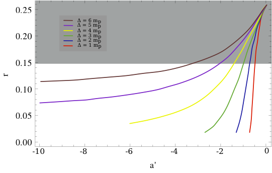
Figure 1: $r$ vs $a^{\prime}$ for several values of $\Delta$. The region in gray is excluded by Planck

In FIG. 2 we present our results for $n_{S}$ and $r$ in a plot confronting $n_{s}$ with $r$ for $\Delta=3m_{P}$ and $a^{\prime}$ obeying the values corresponding to the green curve in FIG. 1 for several e-fold values. As we can see in that plot, the model predictions for $n_{S}$ and $r$ are in perfect agreement with the experimental bounds provided by PLANCK2015. This result is valid for any other choice of the values for the parameter $\Delta$ presented in FIG. 1.

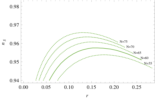
Figure 2: $n_{S}$ vs $r$ for $\Delta=3m_{P}$.

Another interesting outcome we have obtained concerns the inflaton mass. Its expression at tree level is extracted from the diagonalization of the mass matrix $M_{R}^{2}$ in Eq. (40). As reheating demands very tiny $\lambda_{\phi}$ and $v_{\phi}\gg v_{\rho}\,,\,v_{\eta}\,,\,v_{\chi^{\prime}}$, then the $(M_{R}^{2})_{44}$ element of that matrix decouples incurring into the following expression for the inflaton mass at tree level, $m_{\Phi}\sim\sqrt{2\lambda_{10}}v_{\phi}$. When radiative corrections are plugged in, this expression receives a correction that depends on the parameters $a^{\prime}$ and $\Delta$. In FIG. 3 we plot the behaviour of the inflaton mass $m_{\Phi}$ with $a^{\prime}$ for some values of $\Delta$. Even if $v_{\phi}$ is around $10^{10}$ GeV, but as the coupling $\lambda_{10}$ is very small, as required by reheating phase, the inflaton gains a small mass when compared to the conventional chaotic inflation case. According to the prediction of our model, the inflaton may develop mass until few tens of TeV. This has implications to the reheating phase, as discussed below.

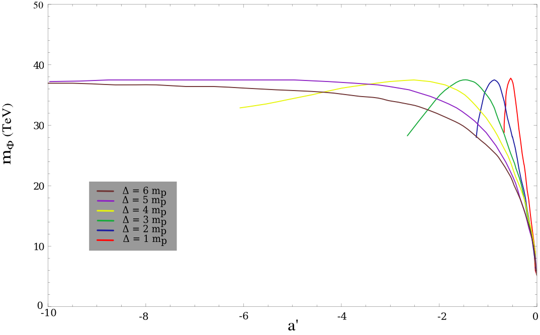
Figure 3: $m_{\phi}$ vs $a^{\prime}$ for several values of $\Delta$.

For sake of completeness, in FIG. 4 we plot the running index $\alpha$ versus $n_{S}$ for some values of $\Delta$. There we have a relatively small $\alpha$ value for all points as it has to be in chaotic inflation.

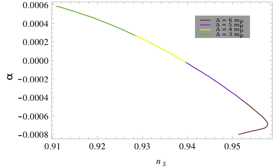
Figure 4: $\alpha$ vs $n_{S}$ for several values of $\Delta$.

We finish this section by discussing reheating Abbott et al. (1982). First of all notice that our inflaton couples to the heavy neutrinos through the Yukawa coupling in Eq. (26), and to scalars through the last four terms in the potential in Eq. (41). Because $v_{\phi}\sim 10^{10}$ GeV, the inflaton develops mass around tens of TeV, as shown in FIG. 3. This order of magnitude for the inflaton mass forbids that it decays into a pair of heavy neutrinos once, as we will see below, $m_{N_{R}}\sim 10^{7}$ GeV. Thus reheating will be solely due to the decay of the inflaton into a pair of scalars.

The 3-3-1 model in question involves several scalars, which makes it very difficult to analytically obtain the scalars in the physical basis. Because of this we just estimate the reheating temperature that may be achieved in our model.

Even with the inflaton decaying into a pair of scalars only, it does not face trouble in reheating the universe until temperatures around $10^{9}$ GeV which is the highest temperature that does not present the gravitino problem. For our proposal it is just enough to parameterize the coupling among the inflaton and a pair of Higgs, provided by those last four terms in the potential in Eq. (41), by the general form: $\frac{\lambda}{8}v_{\phi}\Phi hh$. According to this coupling, we obtain,

$$\Gamma(\Phi\rightarrow hh)\sim\frac{\lambda^{2}v^{2}_{\phi}}{32\pi m_{\Phi}}.$$ (50)

As it is well known the reheating temperature is estimated to be

$$T_{R}\sim 0.1\sqrt{\Gamma(\Phi\rightarrow hh)m_{P}}.$$ (51)

For $v_{\phi}=10^{10}$ GeV and $m_{\Phi}\sim 10$ TeV, a reheating temperature around $10^{9}$ GeV requires $\lambda\sim 10^{-6}$. This means that the couplings $\lambda_{\phi\,,\,11\,,\,12\,,\,13}$ must must be around this order of magnitude. Such tiny values for these couplings is typical in chaotic inflation models. In summary, in spite of the fact that the inflaton has an unusual small mass, the model is efficient in reheating the universe.

IV Some remarks and conclusions

When $\eta^{0}$ and $\phi$ develop VEVs, the last two terms in the Lagrangian in Eq. (26) yields Dirac and Majorana mass terms for $\nu_{L}$ and $N_{R}$,

$${\cal L}\supset M_{D}\bar{\nu}_{L}N_{R}+M\bar{N}^{C}_{R}N_{R}+H.c.,$$ (52)

where $M_{D}=h\frac{v_{\eta}}{\sqrt{2}}$ and $M=\frac{h^{\prime}v_{\phi}}{\sqrt{2}}$. These terms provides the following mass matrix for the six massive neutrino,

$$M_{\nu}=\begin{pmatrix}0&M_{D}\\ M^{T}_{D}&M\end{pmatrix}.$$ (53)

This is the well known mass matrix for the type I seesaw mechanism whose the diagonalization, for $M\gg M_{D}$, leads to Gell-Mann et al. (1979)Mohapatra and Senjanovic (1980),

$$m_{\nu_{L}}\simeq\frac{M^{2}_{D}}{M}\,\,\,\,\,\,\,\mbox{and}\,\,\,\,\,\\ ,\,M_{R}\simeq M.$$ (54)

Here we are interested only in getting an estimate on its order of magnitude. As $a^{\prime}\approx\frac{a}{32\pi^{2}\lambda^{\prime}}$ and $a=-16h^{\prime 4}$, for $a^{\prime}$ around $10$ and $\lambda^{\prime}\sim 10^{-14}$, as required by $\Delta^{2}_{R}=2.215\times 10^{-9}$, we get $h^{\prime}\sim 10^{-3}$, which results in $M_{R}\sim 10^{7}$ GeV. So as to obtain heavy neutrinos with such a mass and standard neutrinos at eV scale, in agreement with solar and atmospheric neutrino oscillation, we just need $M_{D}\sim(10^{-1}-10^{-2})$ GeV. This is obtained for $h$ in the range $\sim(10^{-3}-10^{-4})$ for $v_{\eta}\sim 10^{2}$ GeV. Such range of values for $h$ are of the same order of the average Yukawa couplings in the standard model.

Axion dark matter is considered as an attractive alternative to thermal WIMP dark matter. Our axion is invisible and receives mass through chiral anomaly, $m^{2}_{\mbox{axion}}\sim\frac{\Lambda^{4}_{QCD}}{f^{2}_{pq}}$, which gives mass around $10^{-3}$ eV for $f_{pq}\sim 10^{10}$ GeV and $\Lambda_{QCD}\sim 10^{-1}$ GeV, turning our axion a natural candidate for cold dark matter. As PQ symmetry is broken during inflation, our axion will be produced in the early universe through the misalignment mechanism and its relic abundance is cast in Refs. Turner and Wilczek (1991) Linde (1991).

Just few words about heavy neutrinos with masses around $10^{7}$ GeV. These neutrinos interact with charged scalars, as allowed by the Yukawa coupling $h\bar{f}_{L}\eta N_{R}$, and may give rise to baryogenesis through leptogenesis. Because of the complexity and importance of such subject, we treat it separately elsewhere. However, for a previous treatment of this issue in a similar situation, but different scenario, we refer the reader to the Ref. Huong et al. (2015) .

In summary, several papers have proposed extensions of the standard model that provide a common origin to the understanding of the strong CP-problem, dark matter, inflation, and small neutrino masses. In this paper we argued that such proposal is elegantly realized in the framework of a 3-3-1 gauge model. In it the strong CP-problem is solved with the PQ symmetry whose associated axion is invisible and may constitute the dark matter of the universe. Inflation is driven by the real part of the neutral scalar singlet that contains the axion. Successful inflation was obtained by considering radiative corrections to the inflaton potential. The model predicts an inflaton with mass of tens of GeV that may be probed in a future 100 TeV proton-proton colision. Reheating is achieved through the decay of the inflaton into scalars, solely and neutrinos gain small mass through the type I seesaw mechanism.

References

• Frampton (1992) P. H. Frampton, Phys. Rev. Lett. 69, 2889 (1992).
• de Sousa Pires and Ravinez (1998) C. A. de Sousa Pires and O. P. Ravinez, Phys. Rev. D58, 035008 (1998), [Phys. Rev.D58,35008(1998)], eprint hep-ph/9803409.
• de Sousa Pires (1999) C. A. de Sousa Pires, Phys. Rev. D60, 075013 (1999), eprint hep-ph/9902406.
• Pal (1995) P. B. Pal, Phys. Rev. D52, 1659 (1995), eprint hep-ph/9411406.
• Weinberg (1978) S. Weinberg, Phys. Rev. Lett. 40, 223 (1978).
• Wilczek (1978) F. Wilczek, Phys. Rev. Lett. 40, 279 (1978).
• Kim (1979) J. E. Kim, Phys. Rev. Lett. 43, 103 (1979).
• Shifman et al. (1980) M. A. Shifman, A. I. Vainshtein, and V. I. Zakharov, Nucl. Phys. B166, 493 (1980).
• Dine et al. (1981) M. Dine, W. Fischler, and M. Srednicki, Phys. Lett. B104, 199 (1981).
• Montero et al. (2002) J. C. Montero, C. A. De S. Pires, and V. Pleitez, Phys. Rev. D65, 095001 (2002), eprint hep-ph/0112246.
• Dias et al. (2012) A. G. Dias, C. A. de S. Pires, P. S. Rodrigues da Silva, and A. Sampieri, Phys. Rev. D86, 035007 (2012), eprint 1206.2590.
• Dong and Long (2008) P. V. Dong and H. N. Long, Phys. Rev. D77, 057302 (2008), eprint 0801.4196.
• Boucenna et al. (2015) S. M. Boucenna, J. W. F. Valle, and A. Vicente, Phys. Rev. D92, 053001 (2015), eprint 1502.07546.
• de S. Pires and Rodrigues da Silva (2007) C. A. de S. Pires and P. S. Rodrigues da Silva, JCAP 0712, 012 (2007), eprint 0710.2104.
• Mizukoshi et al. (2011) J. K. Mizukoshi, C. A. de S. Pires, F. S. Queiroz, and P. S. Rodrigues da Silva, Phys. Rev. D83, 065024 (2011), eprint 1010.4097.
• Rodrigues da Silva (2014) P. S. Rodrigues da Silva (2014), eprint 1412.8633.
• Dong et al. (2015) P. V. Dong, C. S. Kim, D. V. Soa, and N. T. Thuy, Phys. Rev. D91, 115019 (2015), eprint 1501.04385.
• Huong and Long (2010) D. T. Huong and H. N. Long, Phys. Atom. Nucl. 73, 791 (2010), eprint 0807.2346.
• Long (2015) H. N. Long (2015), eprint 1501.01852.
• Dias et al. (2014) A. G. Dias, A. C. B. Machado, C. C. Nishi, A. Ringwald, and P. Vaudrevange, JHEP 06, 037 (2014), eprint 1403.5760.
• Barenboim and Park (2016) G. Barenboim and W.-I. Park, Phys. Lett. B756, 317 (2016), eprint 1508.00011.
• Ballesteros et al. (2016a) G. Ballesteros, J. Redondo, A. Ringwald, and C. Tamarit (2016a), eprint 1608.05414.
• Ballesteros et al. (2016b) G. Ballesteros, J. Redondo, A. Ringwald, and C. Tamarit (2016b), eprint 1610.01639.
• Ade et al. (2016) P. A. R. Ade et al. (Planck), Astron. Astrophys. 594, A20 (2016), eprint 1502.02114.
• Dias et al. (2003) A. G. Dias, C. A. de S. Pires, and P. S. Rodrigues da Silva, Phys. Rev. D68, 115009 (2003), eprint hep-ph/0309058.
• Singer et al. (1980) M. Singer, J. W. F. Valle, and J. Schechter, Phys. Rev. D22, 738 (1980).
• Montero et al. (1993) J. C. Montero, F. Pisano, and V. Pleitez, Phys. Rev. D47, 2918 (1993), eprint hep-ph/9212271.
• Foot et al. (1994) R. Foot, H. N. Long, and T. A. Tran, Phys. Rev. D50, R34 (1994), eprint hep-ph/9402243.
• Coleman and Weinberg (1973) S. R. Coleman and E. J. Weinberg, Phys. Rev. D7, 1888 (1973).
• Senoguz and Shafi (2008) V. N. Senoguz and Q. Shafi, Phys. Lett. B668, 6 (2008), eprint 0806.2798.
• Boucenna et al. (2014) S. M. Boucenna, S. Morisi, Q. Shafi, and J. W. F. Valle, Phys. Rev. D90, 055023 (2014), eprint 1404.3198.
• Liddle et al. (1994) A. R. Liddle, P. Parsons, and J. D. Barrow, Phys. Rev. D50, 7222 (1994), eprint astro-ph/9408015.
• Lyth and Liddle (2009) D. H. Lyth and A. R. Liddle, The primordial density perturbation: Cosmology, inflation and the origin of structure (2009), URL http://www.cambridge.org/uk/catalogue/catalogue.asp?isbn=9780521828499.
• Abbott et al. (1982) L. F. Abbott, E. Farhi, and M. B. Wise, Phys. Lett. B117, 29 (1982).
• Gell-Mann et al. (1979) M. Gell-Mann, P. Ramond, and R. Slansky, Conf. Proc. C790927, 315 (1979), eprint 1306.4669.
• Mohapatra and Senjanovic (1980) R. N. Mohapatra and G. Senjanovic, Phys. Rev. Lett. 44, 912 (1980).
• Turner and Wilczek (1991) M. S. Turner and F. Wilczek, Phys. Rev. Lett. 66, 5 (1991).
• Linde (1991) A. D. Linde, Phys. Lett. B259, 38 (1991).
• Huong et al. (2015) D. T. Huong, P. V. Dong, C. S. Kim, and N. T. Thuy, Phys. Rev. D91, 055023 (2015), eprint 1501.00543.