Finding the One: Identifying the Host Galaxies of Gravitational-Wave Sources

Abstract

We explore the localization of compact binary coalescences with ground-based gravitational-wave detector networks. We simulate tens of thousands of binary events, and present the distributions of localization sky areas and localization volumes for a range of sources and network configurations. We show that generically there exists a tail of particularly well-localized events, with 2D and 3D localizations of $<10\,\mbox{deg}^{2}$ and $<1000\,\mbox{Mpc}^{3}$ achievable, respectively, starting in LIGO/Virgo’s third observing run. Incorporating estimates for the galaxy density and the binary event rates, we argue that future gravitational-wave detector networks will localize a small number of binary systems per year to a sufficiently small volume that the unique host galaxy might be identified. For these golden events, which are generally the closest and loudest ones, the gravitational-wave detector networks will point (in 3D; the length of the finger matters) directly at the source. This will allow for studies of the properties of the host galaxies of compact binary mergers, which may be an important component in exploring the formation channels of these sources. In addition, since the host will provide an independent measurement of the redshift, this will allow the use of the event as a standard siren to measure cosmology. Furthermore, identification of a small number of host galaxies can enable deep follow-up searches for associated electromagnetic transients.

1. Introduction

The era of gravitational-wave astrophysics has arrived (Abbott et al., 2016f, d), and we now await multi-messenger astronomy to achieve the full scientific potential of these detections. The observation of an electromagnetic (EM) counterpart to a gravitational-wave (GW) source would allow us to more fully characterize and understand the physics and astrophysics of the sources. In addition to direct EM counterparts to the GW events, there is also enormous interest in identifying the host galaxies to these events. For example, measurements of the stellar age, mass, or metallicity of host galaxies, perhaps even as a function of redshift or binary total mass, could lead to major insights and constraints regarding astrophysical formation mechanisms (Abbott et al., 2016b). Furthermore, host galaxies will provide independent estimates of redshift, allowing for the use of gravitational-wave sources as standard sirens (Schutz, 1986). Finally, by identifying a host galaxy we dramatically increase the probability of identifying a transient counterpart associated with the event, since we are then able to utilize sensitive narrow-field instruments to search.

There are two generic ways to identify a host galaxy to a GW event. The first is by detecting a transient counterpart that can be directly associated with the gravitational-wave event. For example, a contemporaneous short gamma-ray burst in a consistent area of the sky and at a consistent distance would be strong evidence for a direct association between the gravitational-wave and the electromagnetic sources. Once the transient is detected, one can often directly identify the host galaxy. This approach has generated enormous interest, spawning a very active EM follow-up community (Abbott et al., 2016e; Soares-Santos et al., 2016; Annis et al., 2016; Cowperthwaite et al., 2016).

An alternate way to identify a host is by examining the three-dimensional localization volume associated with the GW event. As originally noted by Schutz (1986) and later expanded by Del Pozzo (2012), this approach can be used in a statistical fashion: although any individual GW event may have many potential host galaxies within the relevant localization volume, by analyzing many events simultaneously statistical properties of the host galaxies (such as their redshifts) can be inferred. An essential aspect of this approach is the size of the localization volume: the smaller the volume, the smaller the number of potential host galaxies contained within, and the easier the statistical task of identifying the true host. Previous work has indicated that these volumes are $>10^{4}\,\mbox{Mpc}^{3}$, corresponding to $>$hundreds of potential galaxies (Nissanke et al., 2013; Hanna et al., 2014; Gehrels et al., 2016; Singer et al., 2016a, b).

We re-examine the localization volumes associated with sources identified by ground-based gravitational-wave detector networks. We perform a systematic study, incorporating a range of networks and a range of potential sources, and simulate tens of thousands of GW detections. This systematic study takes advantage of the rapid GW localization algorithm described in Chen & Holz (2015) and expanded to 3D in §2. We focus on the loudest events, exploiting the fact that the distribution of detected signal-to-noise ratios is universal (Chen & Holz, 2014) and that loud events can be anticipated and are inevitable, especially these events are generally well-localized (Chen & Holz, 2015). We find that the best localized events, which we call “golden” events, can be constrained to very small volumes, potentially containing only a single galaxy. For these golden events the unique host galaxy may be identified, allowing a direct EM association with the GW source.

We describe our localization algorithm in §2. In §3 we provide an overview of the results, focusing on the dependence of localization volume and area on the GW detector network and the source properties. In §4 we summarize our results and conclude.

2. Methods

We take a Monte Carlo approach, generating a large sample of binary coalescences throughout the Universe and then investigating the fraction which can be detected by various GW networks, and producing the distributions of localizations associated with these detections. We generate 1.4$M_{\odot}$–1.4$M_{\odot}$, 10$M_{\odot}$–10$M_{\odot}$, and 30$M_{\odot}$–30$M_{\odot}$ binary mergers at random sky positions with random inclinations and orientations. The waveforms of these mergers were generated using the waveform generator in LALSuite (https://wiki.ligo.org/DASWG/LALSuite). For the 1.4$M_{\odot}$–1.4$M_{\odot}$ binaries we use the TaylorF2 waveform (Yunes et al., 2009), and for the 10$M_{\odot}$–10$M_{\odot}$ and 30$M_{\odot}$–30$M_{\odot}$ binaries we use the IMRPhenomD waveform (Khan et al., 2016). We assume aligned spin and ignore precession; including general spins should not qualitatively change our results, and in general would lead to slightly improved localization (Farr et al., 2016). We consider two GW detector network configurations (HLV and HLVJI) at two different sensitivities (O3 and design). The O3 sensitivity for H and L corresponds to a binary neutron star (BNS) range of 120 Mpc, while for V the range is 60 Mpc (Abbott et al., 2016g). The design sensitivity for all detectors is taken from the “aLIGO” curve in LIGO Document T1500293 (https://dcc.ligo.org/LIGO-T0900288/public), corresponding to a BNS range of 200 Mpc. Using these waveforms and detector sensitivities we calculate the optimal match filter signal-to-noise ratio (SNR), $\rho$, at each detector:

$$\rho=\left(\displaystyle\int_{f_{\rm low}}^{f_{\rm high}}\frac{|\tilde{h}(f)|^{2}}{S_{h}(f)}\,df\right)^{1/2},$$ (1)

where $\tilde{h}(f)$ is the Fourier transform of the waveform in the frequency domain and $S_{h}(f)$ is the detector power spectral density. We add Gaussian noise of width 1 to the SNR, and calculate the network SNR as the root-sum-square of the noise-added individual detector SNRs. Our detection threshold requires that the network SNR be greater than 12. The cumulative distribution of the luminosity distance of the detected events is shown in Fig. 1; note the tails to nearby events for all scenarios. For detectable events we calculate the time-of-arrival difference and phase difference between pairs of detectors, and add in Gaussian errors following the Fisher matrix formalism (Cutler & Flanagan, 1994).

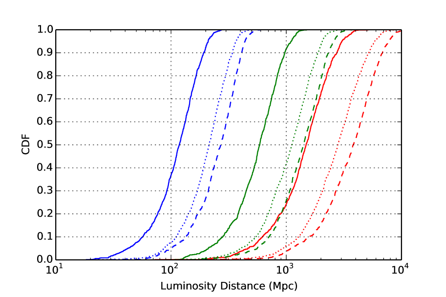
Figure 1.— Cumulative distribution of the luminosity distances for the simulated detectable 1.4$M_{\odot}$–1.4$M_{\odot}$ (blue), 10$M_{\odot}$–10$M_{\odot}$ (green), and 30$M_{\odot}$–30$M_{\odot}$ (red) binary mergers localized in this paper. We consider three GW detector network configurations at different sensitivities: Solid–HLV at O3 sensitivity, dotted–HLV at design sensitivity, and dashed–HLVJI at design sensitivity. There are 10,000 simulated detectable/localized events for each type of binary systems and network configurations.

In order to localize the source we follow a similar approach to our previous work (Chen & Holz, 2015). We use the measured difference in arrival time, $\Delta t$, the measured difference in phase, $\Delta\eta$, and the measured SNR in the individual detectors to reconstruct the 3D location of the source, $(\theta,\phi,D_{L})$:

$$f(\theta,\phi,D_{L}|\Delta t,\Delta\eta,\rho)=\frac{f(\Delta t,\Delta\eta,\rho|\theta,\phi,D_{L})\,f(\theta,\phi,D_{L})}{f(\Delta t,\Delta\eta,\rho)}.$$ (2)

In our simulations the binary mergers are distributed uniformly in comoving volume and the cosmological parameters are taken to be $(\Omega_{m}=0.27,\Omega_{\Lambda}=0.73,h=0.71)$. Our prior, $f(\theta,\phi,D_{L})$, assumes the same cosmological parameters, and is also uniform in comoving volume. To calculate the posterior in Eq. 2, we grid the sky using healpix pixels (http://healpix.jpl.nasa.gov) and 400 bins in luminosity distance. We scale the resolution in sky direction and luminosity distance depending on the measured SNR of the events. Higher SNR events have finer resolution (e.g., $N_{\rm side}=1024$ for network SNR of 110). The likelihood function $f(\Delta t,\Delta\eta,\rho|\theta,\phi,D_{L})$ is estimated using similar $\chi^{2}$ likelihood methods to those presented in Chen & Holz (2015). For each binary above the network detection threshold we produce a joint likelihood in sky position and distance. For each voxel (3D volume pixel) we produce a probability. We then rank order the probabilities, and starting with the highest probability voxel we sum until we have reached the desired probability threshold. In this manner we produce the 90% likelihood volumes presented in §3. We take the 3D likelihood and project it to obtain the 2D sky localization. Similarly, we then rank the 2D pixels to produce the 90% likelihood localization areas.

In order to verify our algorithm we have produced a “P-P plot”, similar to the verification presented in Chen & Holz (2015), and found our algorithm is working as expected. We have also compared our algorithm to LALInference (Veitch et al., 2015), a code designed to sample the posterior distribution for all source parameters using full models of the source waveform and all detector data, and find good agreement.

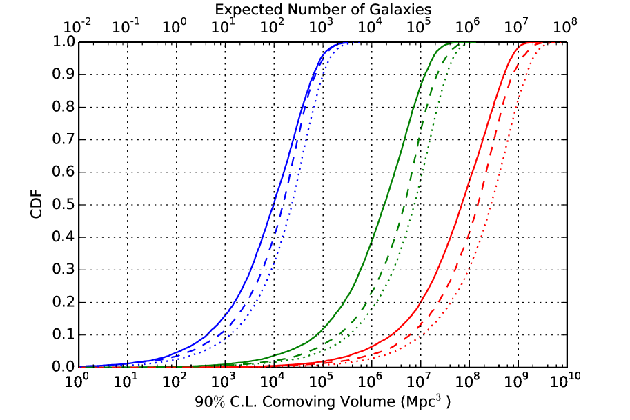
Figure 2.— Cumulative distribution of the 90$\%$ confidence level 3D localization comoving volumes for 10,000 simulated 1.4$M_{\odot}$–1.4$M_{\odot}$ (blue), 10$M_{\odot}$–10$M_{\odot}$ (green), and 30$M_{\odot}$–30$M_{\odot}$ (red) binary mergers. We consider three GW detector network configurations at different sensitivities: Solid–HLV at O3 sensitivity, dotted–HLV at design sensitivity, and dashed–HLVJI at design sensitivity. The top axis shows the expected number of galaxies within the volume assuming the number density of galaxies is 0.01/Mpc³

3. results

Our results are summarized in Figs. 2 and 3 and Tables 1 and 2. Fig. 2 shows a plot of the cumulative distribution of the 90% localization volumes, while Fig. 3 presents the cumulative distribution of 90% localization sky areas. For example, we find that 50% of the BNS sources will be localized to a volume of $\sim 10^{4}\,\mbox{Mpc}^{3}$, regardless of detector network.

We are particularly interested in the number of galaxies that can be expected in these volumes. To estimate this, we assume that the number density of galaxies is 0.01/Mpc³. This estimate takes the Schechter function (Schechter, 1976) parameters in B-band $\phi_{*}=1.6\times 10^{-2}h^{3}$ Mpc^-3, $\alpha$=-1.07, $L_{*}=1.2\times 10^{10}h^{-2}L_{B,\odot}$ and $h=0.7$ ( Norberg et al. (2002); Liske et al. (2003); González et al. (2006); Gehrels et al. (2016), $L_{B,\odot}$ is the solar luminosity in B-band), integrating down to $0.12\,L^{*}$ and comprising 86% of the total luminosity. The top axis in Fig. 2 shows the expected number of galaxies in the 90% localization volumes. For example, a localization volume of 1000 Mpc³ corresponds to an expectation of 10 galaxies, while a localization smaller than 100 Mpc³ corresponds to on average a single galaxy within the localization volume. In other words, for GW sources localized to within 100 $\mbox{Mpc}^{3}$, it may be possible to directly identify the host galaxy without the need for an associated EM transient.

We have argued that a small fraction of GW sources are sufficiently well localized to allow for improved constraints on their host galaxies. But how many of these systems will actually be detected? To estimate this we need to know the expected number of systems that will be detected by the various networks. With only a few systems detected to date, the rate of binary coalescences remains uncertain; we assume the rate for (1.4, 1.4), (10, 10), and (30, 30) $M_{\odot}$ binary mergers to be [low, mean, high]: $[10^{-8},10^{-6},10^{-5}]$, $[1\times 10^{-8},5\times 10^{-8},2\times 10^{-7}]$, and $[6\times 10^{-9},2\times 10^{-8},6\times 10^{-8}]$ Mpc^-3yr^-1, respectively (Abadie et al., 2010; Abbott et al., 2016h, c, a). From these rates we are able to estimate the number of systems that will be detected with each GW network, and then use the results in Fig. 2 to infer the number of systems that will be localized sufficiently to identify the unique host galaxy. We summarize our results in Tables 1 and 2.

Network	Mass($M_{\odot}$)	Median (Mpc3)	$<100$ Mpc3 ($\%$)	$<100$ Mpc3 ($\left<{N_{\rm event}}\right>$)	$<1000$ Mpc3 ($\%$)	$<1000$ Mpc3 ($\left<{N_{\rm event}}\right>$)
HLV O3	(1.4, 1.4)	$9.8\times 10^{3}$	4.6	[0.0024, 0.24, 2.4]	16.1	[0.0083, 0.83, 8.3]
HLV O3	(10, 10)	$1.8\times 10^{6}$	0.3	[0.017, 0.085, 0.34]	1.0	[0.061, 0.34, 1.2]
HLV O3	(30, 30)	$6.9\times 10^{7}$	0.1	[0.021, 0.070, 0.21]	0.1	[0.055, 0.18, 0.55]
HLV design	(1.4, 1.4)	$2.3\times 10^{4}$	2.4	[0.0078, 0.78, 7.8]	8.9	[0.029, 2.9, 29]
HLV design	(10, 10)	$7.4\times 10^{6}$	0.2	[0.077, 0.38, 1.5]	0.6	[0.21, 1.0, 4.2]
HLV design	(30, 30)	$2.8\times 10^{8}$	0.0	[0.067, 0.22, 0.67]	0.1	[0.27, 0.89, 2.7]
HLVJI design	(1.4, 1.4)	$1.5\times 10^{4}$	3.5	[0.023, 2.3, 23]	11.5	[0.076, 7.6, 76]
HLVJI design	(10, 10)	$4.6\times 10^{6}$	0.2	[0.13, 0.66, 2.6]	0.7	[0.51, 2.5, 10]
HLVJI design	(30, 30)	$1.5\times 10^{8}$	0.0	[0.043, 0.14, 0.43]	0.1	[0.60, 2.0, 6.0]

Table 1 90$\%$ confidence level 3D localization comoving volumes. First column: detector network and sensitivity. Second column: mass of the binaries. Third column: median 90$\%$ confidence level localization volume. Fourth & sixth columns: fraction of events localized within 100 and 1000 Mpc³. Fifth & seventh columns: expected number of events localized within 100 and 1000 Mpc³ for [low, mean, high] event rate densities, where the intrinsic rate densities of (1.4, 1.4), (10, 10), and (30, 30) $M_{\odot}$ binary mergers are taken to be $[10^{-8},10^{-6},10^{-5}]$, $[1\times 10^{-8},5\times 10^{-8},2\times 10^{-7}]$, and $[6\times 10^{-9},2\times 10^{-8},6\times 10^{-8}]$ Mpc^-3yr^-1, respectively. The run duration for O3 and design are taken to be 9 months and 1 year. The duty cycle is not considered in this calculation (i.e.,it is taken to be 100%).

There are a number of interesting aspects of our results:

• 

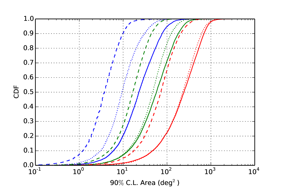
  Figure 3.— Cumulative distribution of the 90$\%$ confidence level 2D localization areas for 10,000 simulated 1.4$M_{\odot}$–1.4$M_{\odot}$ (blue), 10$M_{\odot}$–10$M_{\odot}$ (green), and 30$M_{\odot}$–30$M_{\odot}$ (red) binary mergers. We consider three GW detector network configurations at different sensitivities: Solid–HLV at O3 sensitivity, dotted–HLV at design sensitivity, and dashed–HLVJI at design sensitivity.

• The localization volumes are larger for more massive binaries. This is because these binaries are generally detected to higher distances, and therefore a fractional error in distance or sky position corresponds to a larger volume. Massive binaries also merge at lower frequency and spend shorter time in the GW detectable band, leading to a larger error in estimates of the time-of-arrival. We find that BNS systems are the most likely to be well localized, and therefore are the most likely to allow for unique host galaxy association.

• The localization areas are larger for more massive binaries. Massive binaries are detected at higher distances, so their signals are significantly redshifted and, on top of their intrinsic lower merging frequency, spend even shorter time in band. This is why, for example, the 10-10$M_{\odot}$ binary black hole (BBH) localization area is $\sim$2.5 times that of the BNSs at HLV O3 sensitivity, with the ratio increasing to $\sim$5 at design sensitivity.

• The localization areas are smaller for improved gravitational-wave networks. This is because the localization is primarily dependent on the timing measurements at each detector, and as the networks improve the relative timing improves. Going from three detectors to five detectors causes a large improvement in the 2D localization.

• In all cases there is a tail to very well localized events, corresponding to events that are particularly loud and are fortuitously oriented and located on the sky. For example, for BNS events localized within 1000 $\,\mbox{Mpc}^{3}$ by HLV design sensitivity, the average measured network SNR is 37.

• We find that $\sim 16\%$ of BNS sources detected with the HLV network in O3 will be localized to within 1,000$\,\mbox{Mpc}^{3}$, corresponding to $<10$ galaxies within the 90% localization volume. One in 20 sources will be localized to within 100$\,\mbox{Mpc}^{3}$, indicating that a unique host galaxy may be identified for these events. These values become 2%/9% (at 100/1,000$\,\mbox{Mpc}^{3}$) for HLV at design sensitivity, and 4%/12% at HLVJI at design sensitivity.

• We find that a large fraction of BNS systems are 2D localized to better than 10 deg² for all network configurations; for HLVJI over 90% of sources are localized this well, with almost 10% localized to within 1 deg². The population of well-localized 2D systems overlaps significantly with the population of well-localized 3D systems; these are the high-SNR tail of the universal distribution.

• As the networks improve the fraction of well-localized events can drop as increasing numbers of sources are detected at increasing distance. However, the total number of golden events will increase, since a golden event for a given network will only become “more golden” when detected by an improved network.

• We find that for all network configurations there is an expectation of $\sim 1$ golden event per year: a binary localized to a sufficiently small volume that a unique galaxy host may be identified.

4. Discussion

Network	Mass($M_{\odot}$)	Median (deg2)	$<1$ deg2 ($\%$)	$<1$ deg2 ($\left<{N_{\rm event}}\right>$)	$<10$ deg2 ($\%$)	$<10$ deg2 ($\left<{N_{\rm event}}\right>$)
HLV O3	(1.4, 1.4)	23	0.6	[0.00033, 0.033, 0.33]	20.4	[0.011, 1.1, 11]
HLV O3	(10, 10)	57	0.2	[0.012, 0.058, 0.23]	7.1	[0.43, 2.1, 8.6]
HLV O3	(30, 30)	242	0.1	[0.021, 0.070, 0.21]	1.6	[0.68, 2.3, 6.8]
HLV design	(1.4, 1.4)	9	2.0	[0.0065, 0.65, 6.5]	52.5	[0.17, 17, 170]
HLV design	(10, 10)	47	0.3	[0.12, 0.59, 2.3]	7.5	[2.8, 14, 55]
HLV design	(30, 30)	228	0.0	[0.089, 0.30, 0.89]	1.2	[2.6, 8.7, 26]
HLVJI design	(1.4, 1.4)	4	7.8	[0.052, 5.2, 52]	90.2	[0.60, 60, 597]
HLVJI design	(10, 10)	17	1.1	[0.83, 4.1, 17]	27.5	[20, 101, 403]
HLVJI design	(30, 30)	72	0.2	[0.99, 3.3, 9.9]	4.9	[21, 71, 212]

Table 2 90$\%$ confidence level 2D localization areas. First column: detector network and sensitivity. Second column: mass of the binaries. Third column: median 90$\%$ confidence level localization area. Fourth & sixth columns: fraction of events localized within 1 and 10 deg². Fifth & seventh columns: expected number of events localized within 1 and 10 deg² for [low, mean, high] event rate densities.

We have explored the ability of gravitational-wave detector networks to localize sources both on the sky and in space (sky localization + distance). We have derived the distribution of expected localizations for a range of detector networks and a range of sources. Of particular interest are the cases where the expected number of galaxies is $\left<{N}\right>=1$, since in these cases it is theoretically possible to identify the unique host galaxy associated with a GW sources. We show that in all network configurations there exists a small percentage of sources that will be sufficiently localized so that only a single galaxy may be present in the localization volume. We find that even in O3 there is the likelihood of an event sufficiently well localized such that only a few galaxies will be found within its localization volume, and in the advanced detector era we expect tens of sources per year localized to only a very small number of potential host galaxies, and to be able to uniquely identify the host galaxy of a few sources per year. Figs. 2 and 3 show that localizations deteriorate quickly beyond the first few golden events, suggesting that the utility of this small sample of events may outweigh the rest of the population.

There are a number of potential complications which need to be discussed. We have ignored the role of systematic errors in the GW measurements. For example, a 5% systematic error in the distance estimates will lead to a 5% shift in the 90% confidence volume, and therefore potentially the wrong associated host galaxies. We have performed preliminary tests to show that, given the large spread in distance uncertainties, these effects remain sub-dominant at the 5% level. We have ignored gravitational lensing, since the best localized sources are generally the closest ones. For example, even for the 30–30 $M_{\odot}$ case, the maximum luminosity distance of our sample of binaries localized to within 1,000 Mpc³ is $\sim$400 Mpc. This corresponds to a redshift of $\sim$0.1; gravitational lensing is expected to be negligible at this distance. We note that GW detectors localize sources in luminosity distance, while galaxies generically live in redshift space. In the work above we have assumed a given cosmology to perform this mapping. Since one of our goals is to use these systems as standard sirens to measure cosmological parameters, one may be concerned that our cosmological assumptions preclude independent cosmological measurements. However, if we conservatively assume that the cosmological parameters are known to within 10%, it may nonetheless be possible to narrow down the number of host galaxies. These can then be used in turn to further constrain the cosmological parameters to better than 10% through the use of standard sirens. We have tested this explicitly. In addition, we have ignored the effects of galaxy clustering. Certainly some volumes may center on clusters with a galaxy density orders of magnitude higher than the average. In these cases, identifying the individual host galaxy may become more challenging, although estimating the redshift of the cluster may nonetheless be possible.

Another important complication is the absence of complete galaxy catalogs within the localization volumes of interest. However, we have shown that the associated 2D sky localizations are small for events with well-localized volumes. For example, for BNS events localized by the HLV network at design sensitivity with $\left<{N}\right>\sim 10$ galaxies within their localization volume, the median 90% sky localization area is 1.8 deg². We emphasize that large-field survey telescopes such as the Dark Energy Camera (DECam), Hyper Suprime-Cam, and LSST would be able to fully cover these fields in a small number of pointings. Furthermore, as mentioned above, these well localized systems are the closest ones in the population, and therefore are expected to have correspondingly brighter host galaxies. For example, for the maximum distance of the 30–30 $M_{\odot}$ case discussed above (400 Mpc), the B-band magnitude of a Milky Way-like galaxy would be $\sim 17.6$. Thus an instrument such as DECam would be able to build a complete galaxy catalog in real time across the entire localization region in a few short ($\sim 1\,\mbox{minute}$) pointings. In addition to building an on-the-fly galaxy catalog, the small number of potential host galaxies within the volume coupled with the comparatively nearby distances for these well-localized sources will enable unparalleled triggered searches for EM counterparts. This is further enabled because our 3D localization algorithm presented in §2, as well as the BAYESTAR algorithm presented in Singer et al. (2016a), can be run in low latency ($\sim\,\mbox{minutes}$).

Of particular interest is how these better-localized binaries will impact attempts to measure the Hubble constant with gravitational-wave standard sirens. As far as standard sirens are concerned, identifying a host galaxy is equivalent to identifying an EM counterpart: both cases allow for an independent measurement of the redshift. Although only a small fraction of the sources will be well-localized, since these directly allow for points on the Hubble diagram they provide uniquely powerful constraints (Dalal et al., 2006; Nissanke et al., 2010). We note that the known localization does not significantly improve the distance estimates (Pankow et al., 2016), although we are in the process of exploring this conclusions explicitly for our sample of golden events.

In conclusion, we have shown that there will exist a class of events which will be sufficiently well localized to allow us to narrow the potential number of host galaxies to a small number, and in extreme cases allow for the unique identification of the host of the GW source. These special cases will directly engender multi-messenger astronomy without the need for associated transient EM counterparts. These golden events are likely to be of particular interest in the development of GW astrophysics and cosmology.

References

- Abadie et al. (2010) Abadie, J., Abbott, B. P., Abbott, R., et al. 2010, Classical and Quantum Gravity, 27, 173001
- Abbott et al. (2016a) Abbott, B. P., Abbott, R., Abbott, T. D., et al. 2016a, arXiv:1607.07456, arXiv:1607.07456
- Abbott et al. (2016b) —. 2016b, Astrophys. J. Lett., 818, L22
- Abbott et al. (2016c) —. 2016c, Physical Review X, 6, 041015
- Abbott et al. (2016d) —. 2016d, Physical Review Letters, 116, 241103
- Abbott et al. (2016e) —. 2016e, Astrophys. J. Lett., 826, L13
- Abbott et al. (2016f) —. 2016f, Physical Review Letters, 116, 061102
- Abbott et al. (2016g) —. 2016g, Living Reviews in Relativity, 19, arXiv:1304.0670
- Abbott et al. (2016h) —. 2016h, arXiv:1602.03842, arXiv:1602.03842
- Annis et al. (2016) Annis, J., Soares-Santos, M., Berger, E., et al. 2016, Astrophys. J. Lett., 823, L34
- Chen & Holz (2014) Chen, H.-Y., & Holz, D. E. 2014, arXiv:1409.0522, arXiv:1409.0522
- Chen & Holz (2015) —. 2015, arXiv:1509.00055, arXiv:1509.00055
- Cowperthwaite et al. (2016) Cowperthwaite, P. S., Berger, E., Soares-Santos, M., et al. 2016, Astrophys. J. Lett., 826, L29
- Cutler & Flanagan (1994) Cutler, C., & Flanagan, É. E. 1994, Phys. Rev. D, 49, 2658
- Dalal et al. (2006) Dalal, N., Holz, D. E., Hughes, S. A., & Jain, B. 2006, Phys. Rev. D, 74, 063006
- Del Pozzo (2012) Del Pozzo, W. 2012, Phys. Rev. D, 86, 043011
- Farr et al. (2016) Farr, B., Berry, C. P. L., Farr, W. M., et al. 2016, ApJ, 825, 116
- Gehrels et al. (2016) Gehrels, N., Cannizzo, J. K., Kanner, J., et al. 2016, ApJ, 820, 136
- González et al. (2006) González, R. E., Lares, M., Lambas, D. G., & Valotto, C. 2006, Astron. Astrophys., 445, 51
- Hanna et al. (2014) Hanna, C., Mandel, I., & Vousden, W. 2014, ApJ, 784, 8
- Hughes & Menou (2005) Hughes, S. A., & Menou, K. 2005, ApJ, 623, 689
- Khan et al. (2016) Khan, S., Husa, S., Hannam, M., et al. 2016, Phys. Rev. D, 93, 044007
- Liske et al. (2003) Liske, J., Lemon, D. J., Driver, S. P., Cross, N. J. G., & Couch, W. J. 2003, Mon. Not. R. Astron. Soc., 344, 307
- Nissanke et al. (2010) Nissanke, S., Holz, D. E., Hughes, S. A., Dalal, N., & Sievers, J. L. 2010, Astrophys. J., 725, 496
- Nissanke et al. (2013) Nissanke, S., Kasliwal, M., & Georgieva, A. 2013, ApJ, 767, 124
- Norberg et al. (2002) Norberg, P., Cole, S., Baugh, C. M., et al. 2002, Mon. Not. R. Astron. Soc., 336, 907
- Pankow et al. (2016) Pankow, C., Sampson, L., Perri, L., et al. 2016, ArXiv e-prints, arXiv:1610.05633
- Schechter (1976) Schechter, P. 1976, ApJ, 203, 297
- Schutz (1986) Schutz, B. F. 1986, Nature, 323, 310
- Singer et al. (2016a) Singer, L. P., Chen, H.-Y., Holz, D. E., et al. 2016a, Astrophys. J. Lett., 829, L15
- Singer et al. (2016b) —. 2016b, Astrophys. J.s, 226, 10
- Soares-Santos et al. (2016) Soares-Santos, M., Kessler, R., Berger, E., et al. 2016, Astrophys. J. Lett., 823, L33
- Veitch et al. (2015) Veitch, J., Raymond, V., Farr, B., et al. 2015, Phys. Rev. D, 91, 042003
- Yunes et al. (2009) Yunes, N., Arun, K. G., Berti, E., & Will, C. M. 2009, Phys. Rev. D, 80, 084001