Dipole-dipole dispersion interactions between neutrons

Abstract

We investigate the long-range interactions between two neutrons utilizing recent data on the neutron static and dynamic electric and magnetic dipole polarizabilities. The resulting long-range potentials are used to make quantitative comparisons between the collisions of a neutron with a neutron and a neutron with a proton. We also assess the importance of the first pion production threshold and first excited state of the nucleon, the $\Delta$-resonance ($J^{\pi}$ = + 3/2, I = 3/2). We found both dynamical effects to be quite relevant for distances $r$ between $\sim 50$ fm up to $\sim 10^{3}$ fm in the nn system, the neutron-wall system and in the wall-neutron-wall system, reaching the expected asymptotic limit beyond that. Relevance of our findings to the confinement of ultra cold neutrons inside bottles is discussed.

I Introduction

A polarizable particle is expected to exhibit a long-range electromagnetic interaction. Examples include the charge-induced dipole interaction energy between an electron and a hydrogen atom, $-\frac{1}{2}\alpha e^{2}/d^{4}$, and the dipole-dipole dispersion interaction energy between two hydrogen atoms, $-C_{6}/d^{6}$, where $d$ is the separation between the electron and the H atom or between the two H atoms, $\alpha=\frac{9}{2}a_{0}^{3}$ is the atomic electric dipole polarizability, and $C_{6}\approx 6.5e^{2}a_{0}^{5}$ is the dispersion or van der Waals constant. The quantities $\alpha$ and $C_{6}$ can be expressed in terms of the electric dipole oscillator strength distribution of the atom, which describes the response of the electron to photons at specific frequencies of an external electric field. Higher order interaction energies involving magnetic dipole and higher-order multipolar polarizabilities, and multipolar dispersion constants are also well-characterized and these may be expressed in terms of the corresponding multipolar oscillator strengths. These interaction potentials are general for atoms and molecules and they are widely studied and applied for descriptions of spectroscopy and scattering.

The neutron possesses internal structure (two quarks down and one quark up) with an electric dipole polarizability $\alpha_{n}$ and a magnetic dipole polarizability $\beta_{n}$, usually viewed as the response of the pion cloud to external electromagnetic fields SchRauRie89 ; WisLevSch98 ; GriMcGPhi12 ; HolSch14 . The most recent recommended values from the Particle Data Group (PDG) are $\alpha_{n}=(11.6\pm 1.5)\times 10^{-4}$ fm³ and $\beta_{n}=(3.7\pm 2.0)\times 10^{-4}$ fm³ pdg . Another recommendation is $\alpha_{n}=(12.5\pm 1.8)\times 10^{-4}\;\textrm{fm}^{3}$ and $\beta_{n}=(2.7\mp 1.8)\times 10^{-4}\;\textrm{fm}^{3}$ KosCamWis03 . (The appearance of $\pm$ and $\mp$ is related to the sum rule used to determine these values.) A number of separate groups determined the neutron electric dipole polarizability $\alpha_{n}$ by measuring the effect of the potential energy

$$-\textstyle{\frac{1}{2}}\alpha_{n}e^{2}Z^{2}/R^{4},$$ (1)

where $Z$ is the nuclear charge and $R$ is the separation distance, on the scattering amplitude Tha59 in neutron scattering by ${}^{208}\textrm{Pb}$ nuclei. The high nuclear charge generates an electric field that polarizes the neutron leading to an effect completely analogous and of the same form as that mentioned in the first paragraph for the charge-induced dipole interaction between an electron and an atom. Experiments were carried out looking at the differential scattering of neutrons on Pb and by looking at neutron transmission through Pb. For example, using neutron transmission through lead Schmiedmayer et al. SchRieHar91 obtained the value $\alpha_{n}=(12.0\pm 1.5\pm 2.0)\times 10^{-4}$ fm³, where the first uncertainty is statistical and the second uncertainty is systematical. Further analyses of this experiment and discussions of other neutron-nucleus scattering experiments can be found in Refs. Ale96 ; WisLevSch98 ; Pok00 . Two other experimental approaches to the neutron polarizability are through measurements of quasi-free Compton scattering from the bound neutron in the deuteron ($\gamma+\textrm{d(np)}\rightarrow\gamma^{\prime}+\textrm{d(np)}$) and of elastic photon scattering from the deuteron ($\gamma+\textrm{d}\rightarrow\gamma+\textrm{d}$) DrePasVan03 ; Hagelstein:2015egb , where the observable quantities are the Compton polarizabilities $\bar{\alpha}_{n}+\bar{\beta}_{n}$ and $\bar{\alpha}_{n}-\bar{\beta_{n}}$. In particular, Compton scattering experimental results, with the use of sum rules, led to the recommended values for $\beta_{n}$, cited above. One can also use sum rules and the result for $\alpha_{n}$ from neutron scattering experiments to determine $\beta_{n}$ SchRieHar91 ; Hagelstein:2015egb . Compton scattering implies a response of the neutron to photon energies and provides a connection to the polarizabilities. Care is required in using theoretical Compton scattering frequency-dependent amplitudes because of the presence of relatively small corrections arising from the relativistic wave equations utilized Pet64 ; KarMil99 , but no conceptual difficulties arise in relating static polarizabilities arising in Compton scattering to those arising from an external electric field because they are identical KosCamWis03 ; Sch05 . In the past few years the frequency-dependent values of $\alpha_{n}$ and $\beta_{n}$ have been calculated in the framework of chiral effective field theory Hil05 ; GriMcGPhi12 ; Lensky:2012ag ; Hagelstein:2015egb , the effective theory of the underlying quantum chromodynamics (QCD). Guided by the approximate chiral symmetry of QCD, these calculations show good agreement with data, though convergence patterns are different depending on its covariant or heavy-baryon formulations, and on the explicit inclusion of the Delta resonance (c.f. Ref. Lensky:2012ag ).

The paper addresses the influence of the internal structure of the neutron and proton on their dispersive interactions with another neutron. In the second section we look at the neutron-neutron Casimir-Polder (CP) interaction and in the third section we compare the CP effect in the nn and pn systems. In the fourth section we derive the CP interaction in the neutron-wall system, and finally in the fifth section, we give our concluding remarks.

II The neutron-neutron Casimir-Polder interaction

We believe it is reasonable to expect that there is a neutron-neutron dispersion interaction, based on the experimental evidence for the static polarizabilities $\alpha_{n}$ and $\beta_{n}$ and on theoretical calculations of the polarizabilities as functions of photon energies. Indeed, while our conclusion is based on a physical analogy between the neutron and the H atom there is a more formal basis for such an expectation. Feinberg and Sucher showed that for asymptotically large separations, retarded dispersion interactions between two “systems” (electromagnetically polarizable particles) result independently of the system models and follow from general principles of Lorentz invariance, electromagnetic current conservation, analyticity, and unitarity FeiSuc70 ; FeiSuc79 . An early application of these ideas to a calculation of the neutron-neutron scattering length was carried out by Arnold Arn73 . However, at the time of his analysis $\beta_{n}$ was unknown, the accepted value of $\alpha_{n}$ was twice today’s value, and dynamic polarizabilities were unavailable.

Following Feinberg and Sucher FeiSuc70 , the asymptotic ($r\sim\infty$) long-range interaction potential between two neutrons is given by the Casimir-Polder potential

$$V^{\infty}_{CP,nn}(r)=-(\hbar c/4\pi)[23(\alpha_{n}^{2}+\beta_{n}^{2})-14\alpha_{n}\beta_{n}]{r^{-7}}+\mathcal{O}(r^{-9})=V^{*}_{CP,nn}(r)+\mathcal{O}(r^{-9}),$$ (2)

with the notation $V^{*}_{CP}$ meaning the static limit of the nucleon dynamic polarizabilities. In contrast, the asymptotic long-range interaction potential between a proton and a neutron is the sum of the charge-induced dipole interaction potential and the Casimir-Polder-type potential for a neutral polarizable particle and a charged particle BerTar76

$$V^{\infty}_{CP,pn}(r)=\hbar c\,\alpha_{0}\left[-\frac{1}{2}\alpha_{n}r^{-4}+\frac{1}{4\pi cM_{p}}(11\alpha_{n}+5\beta_{n})r^{-5}+\mathcal{O}(r^{-7})\right]=V^{*}_{CP,pn}(r)+\mathcal{O}(r^{-7}),$$ (3)

where $M_{p}$ is the proton mass and $\alpha_{0}=e^{2}/4\pi\sim 1/137$ is the electromagnetic fine structure constant. Note the appearance of a repulsive $r^{-5}$ potential for the asymptotic interaction of a neutron and a proton. (We would expect the polarizability of the proton to enter at the higher order of $\mathcal{O}(r^{-7})$ through a potential similar to Eq. (2) that is bilinear in neutron and proton polarizabilities FeiSuc70 .)

Accordingly, estimates that improve on the asymptotic Casimir-Polder interaction between two neutrons and between a neutron and a proton can be obtained from, respectively, Eqs. (2) and (3), where we have substituted the accepted polarizability values and converted the expressions to suitable units for nuclear physics,

$$V^{*}_{CP,nn}(r)\approx-0.49\times 10^{-3}(r/\textrm{fm})^{-7}\;\textrm{MeV},\quad r\sim\infty,$$ (4)

and

$$V^{*}_{CP,pn}(r)\approx 0.91\times 10^{-3}(r/\textrm{fm})^{-4}[-1+0.40(r/\textrm{fm})^{-1}]\;\textrm{MeV},\quad r\sim\infty.$$ (5)

More generally, The Casimir-Polder theory gives the interaction between two identical neutral polarizable particles valid for all distances sufficiently large that exchange forces are negligible FeiSuc70 ; Bab10 ,

$$V_{CP,ij}(r)=-\frac{\alpha_{0}}{\pi r^{6}}I_{ij}(r)$$ (6)

where

$$I_{ij}(r)=\int_{0}^{\infty}d\omega e^{-2\alpha_{0}\omega r}\Big{\{}\big{[}\alpha_{i}(i\omega)\alpha_{j}(i\omega)+\beta_{i}(i\omega)\beta_{j}(i\omega)\big{]}P_{E}(\alpha_{0}\omega r)$$

$$\hskip 71.13188pt+\big{[}\alpha_{i}(i\omega)\beta_{j}(i\omega)+\beta_{i}(i\omega)\alpha_{j}(i\omega)\big{]}P_{M}(\alpha_{0}\omega r)\Big{\}},$$

$$P_{E}(x)=x^{4}+2x^{3}+5x^{2}+6x+3,\qquad P_{M}(x)=-(x^{4}+2x^{3}+x^{2}),$$ (7)

$\alpha_{i}(\omega)$ and $\beta_{i}(\omega)$ are respectively the dynamic electric and magnetic dipole polarizability of particle $i$, similarly for particle $j$ . Detailed analyses of the neutron based on chiral effective field theory, for photon energies up to the excitation of the $\Delta$ resonance are found in Refs. Hildebrandt:2003fm ; Hil05 ; GriMcGPhi12 ; Lensky:2015awa ; Hagelstein:2015egb . The analytic expressions for the neutron polarizabilities are far from simple. However, we attempt to parametrize $\alpha_{n}(\omega)$ and $\beta_{n}(\omega)$ in terms of relatively simple formulas that incorporate the most important low-energy aspects.

Our parametrization for the dynamic electric dipole polarizability reads

$$\alpha_{n}(\omega)=\frac{\alpha_{n}(0)\,\sqrt{(M_{\pi}+a_{1})(2M_{n}+a_{2})}(0.2a_{2})^{2}}{\sqrt{(\sqrt{|M_{\pi}^{2}-\omega^{2}|}+a_{1})(\sqrt{|4M_{n}^{2}-\omega^{2}|}+a_{2})}\big{[}|\omega|^{2}+(0.2a_{2})^{2}\big{]}}\,.$$ (8)

Besides the static electric polarizability $\alpha_{n}(0)$ and the masses of the pion ($M_{\pi}$) and the neutron ($M_{n}$), this expression has two mass parameters $a_{1}$ and $a_{2}$. The parameter $a_{1}$ is formally a higher-order effect, but important to match the correct pion production threshold, which controls the low-energy behavior of $\alpha_{n}(\omega)$ Hildebrandt:2003fm . The square roots in Eq. (8) are an attempt to incorporate the pion production threshold behavior, above which $\alpha_{n}$ develops an imaginary part. This specific form also assumes a smooth and asymptotically decreasing behavior of $\alpha_{n}$ at imaginary frequencies, which is expected from analyticity of the Compton $S$-matrix and used in the construction of our Casimir-Polder potentials. We fit the above expression to the curves of Lensky, McGovern, and Pascalutsa Lensky:2015awa , results from the covariant formulation of baryon chiral effective field theory (CB-$\chi$EFT). In contrast to the non-relativistic, heavy baryon formulation of $\chi$EFT (HB-$\chi$EFT), the former properly takes into account recoil corrections to all orders, which is relevant to correctly describe the threshold behavior due to pion production. For $M_{n}=938.919$ MeV we obtain $M_{\pi}=134.051$ MeV, fairly close to the neutral pion mass (134.98 MeV). The remaining parameters are presented in Table 1. In Set 1 we let $\alpha_{n}(0)$ be a fit parameter, in Set 2 we keep $\alpha_{n}(0)$ fixed to the PDG central value pdg , and in Set 3 we keep $\alpha_{n}(0)$ fixed to the central value of Ref. KosCamWis03 . The quality of the parametrization can be observed on the left panel of Fig. 1, well within the expected theoretical uncertainties (see Refs. Lensky:2015awa ; Hagelstein:2015egb ).

For the dynamic magnetic dipole polarizability we use

$$\beta_{n}(\omega)=\frac{\beta_{n}(0)-b_{1}^{2}\omega^{2}+b_{2}^{3}{\rm Re}(\omega)}{(\omega^{2}-\omega_{\Delta}^{2})^{2}+|\omega^{2}\Gamma_{\Delta}^{2}|}\,,$$ (9)

which incorporates the relevant physics in this quantity, namely, the $\Delta$ resonance. In fact, from the fit parameters $b_{1}$, $b_{2}$, $\omega_{\Delta}$, and $\Gamma_{\Delta}$, the last two are close to the $n$-$\Delta$ mass splitting  and $\Delta$ resonance width, respectively. The term proportional to ${\rm Re}(\omega)$ mimics the onset of an imaginary term in the Compton amplitude above the real photon threshold, that would otherwise be absent below it. As in the $\alpha_{n}$ case, this specific form assumes a smooth and asymptotically decreasing behavior of $\beta_{n}$ at imaginary frequencies. The fitted parameters are shown in Table 1, with $\beta_{n}(0)$ evaluated in analogous way as $\alpha_{n}(0)$ for each Set. One observes very little spread for this quantity among these three different sets. However, we noticed numerically that the contribution of $\beta_{n}(\omega)$ amounts to a decrease of about 10% in the strength of the Casimir-Polder interaction between two neutrons, $V_{CP,nn}(r)$. This CP potential is, therefore, most sensitive to the differences observed in the description of $\alpha_{n}(\omega)$, as we discuss later.

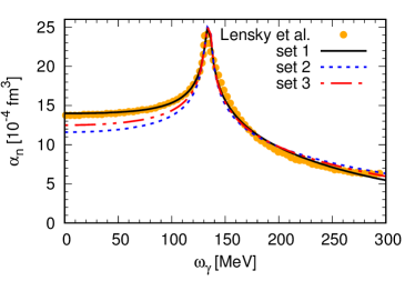
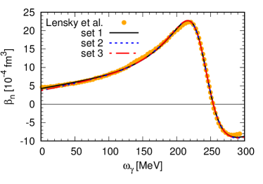
Figure 1: Dynamic electric (left) and magnetic (right) polarizabilities, as functions of the photon energy $\omega_{\gamma}$.

The yellow circles are the CB-$\chi$EFT results of Lensky et al. Lensky:2015awa while sets 1, 2, and 3 correspond to our parametrizations using the numbers specified in Table 1.

	$\alpha_{n}(0)$ ($10^{-4}{\rm fm}^{3}$)	$a_{1}$ (MeV)	$a_{2}$ (MeV)	$\beta_{n}(0)$ ($10^{-4}{\rm fm}^{3}$)	$b_{1}$ (MeV)	$b_{2}$ (MeV)	$\omega_{\Delta}$ (MeV)	$\Gamma_{\Delta}$ (MeV)
Set 1	13.9968	12.2648	1621.63	4.2612	8.33572	22.85	241.484	66.9265
Set 2	11.6	2.2707	2721.47	3.7	8.67962	24.2003	241.593	68.3009
Set 3	12.5	5.91153	2118.79	2.7	9.27719	26.328	241.821	70.8674

Table 1: Parameters of Eqs. (8), (9) fitted to the theoretical curves of Ref. Lensky:2015awa . See text for details.

In order to assess the quality of Eqs. (8), (9) at imaginary frequencies, we compared them to the heavy-baryon chiral EFT (HB-$\chi$EFT) expressions given by Hildebrandt et al., Appendices B and C of Ref. Hildebrandt:2003fm . We made sure to reproduce their results at real $\omega$, then extrapolated to the imaginary domain. HB-$\chi$EFT lies between our set 2 and set 3 with Eq. (8) up to about $i\omega=iM_{\pi}$. On the other hand, for the magnetic case Eq. (9) starts disagreeing with HB-$\chi$PT beyond $i\omega\approx i\,\mathrm{50\,MeV}\sim iM_{\pi}/3$. However, we checked numerically that the magnetic contribution to the Casimir-Polder potentials is at most a 15% effect. We also noticed that the HB-$\chi$EFT results for $\alpha_{n}(i\omega)$ and $\beta_{n}(i\omega)$ exhibit a numerical singularity as one approaches $i\omega=iM_{\pi}$. In such complex-$\omega$ domain the non-Born Compton amplitudes, from which $\alpha_{n}(\omega)$ and $\beta_{n}(\omega)$ are obtained, should not exhibit any low-energy physical singularities. This is probably a consequence of the heavy-baryon formalism in missing the correct pion-production threshold, which is normally fixed “by hand” Hildebrandt:2003fm ; Lensky:2015awa ; Hagelstein:2015egb . In this exploratory work we rely on our parametrizations (8), (9), with room for technical improvements postponed to future works.

Given the dynamic electric (8) and magnetic (9) polarizabilities, one computes the neutron-neutron CP-interaction via Eqs. (6) and (II). Fig. 2 shows the CP-interaction for two neutrons, $V_{CP,nn}(r)$, as a function of the separation distance. The bold red curves correspond to $V_{CP,nn}(r)$ given by the dynamic polarizabilities previously shown, while the thin blue curves correspond to the static limit $\alpha_{n}(\omega)$, $\beta_{n}(\omega)$ $\to$ $\alpha_{n}(0)$, $\beta_{n}(0)$. In such limit, integration of Eq. (II) is straightforward and leads to Eq. (2).

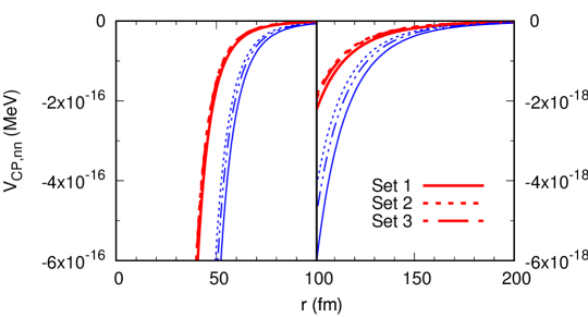
Figure 2: CP-interaction for two neutrons, as a function of the separation distance $r$. The red thick and blue thin lines correspond to the use of dynamical and static dipole polarizabilities, respectively.

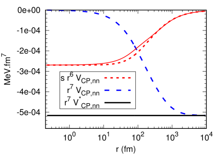
Figure 3: The neutron-neutron CP-interaction as a function of the separation distance $r$, multiplied by $s\,r^{6}$ (red dotted line, with $s=100$ fm) and $r^{7}$ (blue long-dashed line). The black solid line is the CP-potential from the static limit of the dipole polarizabilities, multiplied by $r^{7}$.

The difference between the use of dynamic and static polarizabilities is evident from the curves. In order to assess the expected long-distance limit of Eq. (2) we show $V_{CP,nn}$ in Fig. 3 multiplied by different powers of $r$. We use parameters from Set 3, which illustrates well the qualitative behavior of the other sets. The red dotted curve is the CP potential multiplied by $s\,r^{6}$, where $s=100\,\mathrm{fm}$ to fit in the figure. The blue dashed and black solid lines stand for the dynamic and static polarizabilities versions of $V_{CP,nn}$ (the latter indicated by $V^{*}_{CP,nn}$ in the figure), multiplied by $r^{7}$. The red thin solid line is the arctan parametrization OCaSuc69 , which is utilized in atomic physics (see, for example, Ref. FriJacMei02 ), that makes the transition from the $1/r^{6}$ short-distance van der Waals to the asymptotic $1/r^{7}$ Casimir-Polder behavior Arn73 .

The red dotted curve shows a clear $1/r^{6}$ behavior at small distances up to $\approx 20$ fm, meaning that in this region the integrand of Eq. (II) is nearly constant. This $1/r^{6}$ plateau may be just accidental, since this region is dominated by energies larger than used to set our parametrizations (8), (9). This assertion can be checked via the dominance of the exponential factor of Eq. (II): $r\lesssim 20$ fm receives contributions from neutron excitations larger than $(2\alpha_{0}\times 20\,{\rm fm})^{-1}\sim 670$ MeV. The physics of the Delta resonance appears at about $(2\alpha_{0}\omega_{\Delta})^{-1}\sim 50$ fm, but is minor since it enters mostly via $\beta_{n}(\omega)$, which is numerically of $\sim 10$%. This way, our results can be considered valid for distances beyond 50 fm. On the same reasoning, pion production threshold influences the region around 100 fm. From the blue dashed curve, one also notices that the large distance behavior (2) is only reached beyond $10^{3}$ fm, dominated by dynamic polarizabilities in the region $\omega_{\gamma}\lesssim 10$ MeV.

The above discussion was concentrated on the electromagnetic polarizabilities of the nucleons. The resulting CP interaction is a consequence of two-photon exchange. It is known, though, that the strong interaction also gives rise to long range vdW interaction, the color vdW, arising from multi-gluon exchange. Such force was considered in the scattering of identical heavy nuclei, such as ²⁰⁸Pb, HusLimPat90 , and looked for experimentally VilMitLep93 . Here we mention that this interaction is similar in structure to the electromagnetic one, and can be lumped together.

Considerations of the consequences of the interaction potential power laws $r^{-4}$, $r^{-5}$, $r^{-6}$ and $r^{-7}$ involving neutrons scattering from heavy nuclei were given in Ref. Pok00 , guided by the work of Thaler Tha59 . In the following section we give an account of the influence of our calculated CP interaction in the nn and np systems on the low-energy n-nucleus scattering as done in Pok00 ; Tha59 . We do this for the purpose of completeness and to obtain insights into the way the neutron interacts with the constituents of walls of material which are potentially used in neutron confinements in bottles. The full n-wall and wall-n-wall interactions and potentials will be discussed in the following sections.

III Comparison of the CP effect in the nn and pn scatering systems

The effect of the long range interaction on the neutron-neutron (nn) scattering can be estimated using first order perturbation theory. We can write,

$$f_{nn}(q)=-a_{nn}+f_{nn}^{\infty}(q)$$ (10)

where $a_{nn}$ is the nn scattering length $a_{nn}=-18.9\pm 0.4$ fm. Taking for the neutron wave function a plane wave, $\phi(\bf{k};\bf{r})$ = $\frac{1}{(2\pi)^{3/2}}\exp{(i\bf{k}\cdot\bf{r})}$, the change in the scattering amplitude arising from Eq. (4) is then

$$f_{nn}^{\infty}(q) =-\left(-0.49\times 10^{-3}\,{\rm fm^{7}\cdot MeV}\right)\frac{2\pi^{2}\mu_{nn}}{\hbar^{2}}\int d\textbf{r}\phi^{\star}(\textbf{k}^{\prime};\textbf{r})\frac{1}{r^{7}}\phi(\textbf{k};\textbf{r})$$

$$=\left(0.49\times 10^{-3}\,{\rm fm^{7}\cdot MeV}\right)\frac{M_{n}}{8\pi\hbar^{2}}\int d\textbf{r}e^{i\bf{q}\cdot\bf{r}}\frac{1}{r^{7}}$$ (11)

where $q$ = $|\textbf{k}^{\prime}-\textbf{k}|$ = $2k\sin{(\theta/2)}$ is the momentum transfer divided by $\hbar$, $\mu_{nn}=\textstyle{\frac{1}{2}}M_{n}$ is the reduced mass, and $M_{n}$ is the neutron mass. The integral over r can be performed easily Pok00 . The lower limit of the $r$ integral is set at $r=R$, where $R$ is a radius that characterizes the strong nn interaction and $V_{nn}^{\infty}(r\leq R)=0$. We have,

$$f_{nn}^{\infty}(q)=\left(0.49\times 10^{-3}\,{\rm fm^{7}\cdot MeV}\right)\left(\frac{M_{n}}{2\hbar^{2}}\right)\frac{1}{R^{4}}F_{7}(q)$$ (12)

where

$$F_{7}(q) =\frac{\sin{(qR)}}{5qR}+\frac{\cos{(qR)}}{20}-\frac{qR\sin{(qR)}}{60}-\frac{(qR)^{2}\cos{(qR)}}{120}$$

$$+\frac{(qR)^{3}\sin{(qR)}}{120}+\frac{(qR)^{4}}{120}\int_{qR}^{\infty}dt\frac{\cos{t}}{t}$$ (13)

which gives to leading order in $qR$ the following,

$$F_{7}(q) =\frac{1}{4}-\frac{1}{12}(qR)^{2}$$

$$+\left[\frac{137}{7200}-\frac{\gamma}{120}-\frac{1}{120}\ln{(qR)}\right](qR)^{4}+O((qR)^{6}),$$ (14)

where $\gamma\approx 0.5772$ is Euler-Mascheroni constant.

The cross section is given by $|-a+f_{nn}^{\infty}|^{2}$. Neglecting the term $|f_{nn}^{\infty}|^{2}$, we obtain,

$$\sigma_{nn}(q)=a^{2}-2af_{nn}^{\infty}(q)$$ (15)

A similar analysis can be performed for the proton-neutron (pn) system, using Eq. (5). The amplitude is then given by

$$f_{pn}(q)=-a_{pn}+f_{pn}^{\infty}(q).$$ (16)

Here, $a_{pn}$ is the pn scattering length given by $a_{pn}=-23.74$ fm. The correction owing to the long range interactions is to leading order in $qR$ given by

$$f_{pn}^{\infty}(q) =\left(0.91\times 10^{-3}\,{\rm fm^{4}\cdot MeV}\right)\frac{\mu_{pn}}{4\pi\hbar^{2}}\int d\textbf{r}e^{i\textbf{q}\cdot\textbf{r}}\left[\frac{1}{r^{4}}-\frac{0.40\,{\rm fm}}{r^{5}}\right]$$

$$\approx\left(0.91\times 10^{-3}\,{\rm fm^{4}\cdot MeV}\right)\left(\frac{M_{n}}{2\hbar^{2}}\right)\frac{1}{R}\left[F_{4}(q)-\frac{0.40\,{\rm fm}}{R}F_{5}(q)\right],$$ (17)

where $\mu_{pn}$ is the reduced mass of the proton and neutron and where the functions $F_{4}(q)$ and $F_{5}(q)$ are given by Pok00 ; Tha59

$$F_{4}(q)=1-\frac{1}{4}\pi qR+\frac{1}{6}(qR)^{2}+....$$ (18)

and Pok00

$$F_{5}(q)=\frac{1}{2}-\left[\frac{11}{36}-\frac{\gamma}{6}-\frac{\ln(qR)}{6}\right](qR)^{2}+....$$ (19)

The above results can be summarized by introducing effective scattering lengths for the nn and the np systems. Using the definition $a_{\mathrm{eff.}}=a-f(0)$ we find, for the effective CP-modified scattering length for the $nn$ system,

$$a_{nn,\mathrm{eff.}}=a_{nn}-f_{nn}^{\infty}(0)=a_{nn}-1.23\times 10^{-4}\left(\frac{M_{n}}{2\hbar^{2}}\right)\frac{1}{R^{4}},$$ (20)

and similarly for the $np$ system,

$$a_{pn,\mathrm{eff.}}=a_{np}-f_{np}^{\infty}(0)=a_{np}+0.91\times 10^{-3}\left(\frac{M_{n}}{2\hbar^{2}}\right)\frac{1}{R^{2}}\left(R-0.20\,{\rm fm}\right),$$ (21)

It is clear that the effect of the CP interaction is more pronounced in the np system; basically an order of magnitude stronger. This becomes clear when calculating the relative effect on the corresponding cross sections. This discussion about the effect of the Casimir-Polder interaction on the scattering lengths of nucleon-nucleon system could be of use in the study of charge symmetry violation in hadron physics Miller:2006tv .

It is now a simple undertaking to compare the nn and the pn long-range corrections to the cross sections,

$$\frac{\Delta\sigma_{nn}(q)}{\Delta\sigma_{pn}(q)} =\frac{a_{nn}f_{nn}^{\infty}(q)}{a_{pn}f_{pn}^{\infty}(q)}$$

$$=\frac{0.49\,{\rm fm^{7}\cdot MeV}}{0.91\,{\rm fm^{4}\cdot MeV}}\frac{18.9\,{\rm fm}}{23.74\,{\rm fm}}\left[\frac{F_{7}(q)/R^{3}}{F_{4}(q)-F_{5}(q)\times 0.40\,{\rm fm}/R}\right].$$ (22)

Then,

$$\frac{\Delta\sigma_{nn}(q)}{\Delta\sigma_{pn}(q)}\approx\frac{0.43\,{\rm fm^{3}}}{R^{3}}\left[\frac{\frac{1}{4}-\frac{1}{12}(qR)^{2}}{1-\frac{1}{4}\pi qR+\frac{1}{6}(qR)^{2}-\frac{0.4\,{\rm fm}}{R}\left[\frac{1}{2}-\left(\frac{11}{36}-\frac{\gamma}{6}-\frac{\ln(qR)}{6}\right)\right](qR)^{2}}\right].$$ (23)

Taking for $qR$ the value $1\times 10^{-3}$, with $R=20$ fm and $q=k=5\times 10^{-5}(\mathrm{fm})^{-1}$, corresponding to center of mass nn energy of 1 eV, we can obtain the following numerical estimate.

$$\frac{\Delta\sigma_{nn}(q)}{\Delta\sigma_{pn}(q)}\approx 1.36\times 10^{-5}.$$ (24)

The estimate given above clearly indicates that at very low energies, the np system is much more influenced by the CP interaction than the nn system. Individually, however, both are very little affected by this interaction when discussing neutrons in containers, such as bottles, at energies in the neV region (ultra cold neutrons). The neutrons feel an over all repulsive interaction with the walls of the container arising from the Fermi pseudo potential which becomes operative when a critical neutron energy is reached FerMar47 ; Zel59 . This critical energy varies in value with the material of the wall, but in general it is in the 100’s of neV (e.g. for nickel the critical Fermi energy is 252 neV). In containers with walls of aluminum the Fermi pseudo energy or potential is much lower, about 54 neV, corresponding to neutron velocity of 3-24 m/s. Therefore the CP effect which is repulsive for the pn system, the dominant constituent in the neutron-wall interaction, has an extremely small effect when compared to the dominant Fermi repulsion.

IV The neutron-wall interaction

In discussing the confinement of neutrons inside containers or bottles, one is bound to consider the interaction of neutrons with the wall of the container. The case of an atom and a perfectly conducting wall was considered by Casimir and Polder, and they obtained the following expression valid for very large $r$

$$V_{CP,aW}(r)=-\frac{3}{8\pi}\hbar c\alpha_{d}(0)\frac{1}{r^{4}}\,,$$ (25)

where $\alpha_{d}(0)$ is the dynamic polarizability of the atom at zero frequency. The above formula has been re-derived by many authors and a more general expression was obtained which gives the above as the limiting case as $r\rightarrow\infty$, and a $\frac{1}{r^{3}}$ form for smaller values of $r$. For neutron-wall interaction a similar expression holds and it can be written as khar97

$$V_{CP,nW}(r)=-\frac{\alpha_{0}}{4\pi r^{3}}J_{nW}(r)$$ (26)

where

$$J_{nW}(r)=\int_{0}^{\infty}d\omega\,e^{-2\alpha_{0}\omega r}\alpha_{n}(i\omega)Q(\alpha_{0}\omega r)\,,$$

$$Q(x)=2x^{2}+2x+1\,.$$ (27)

We deduce the neutron-wall interaction based on analogy with the atom-wall interaction describing the long-range potential between a neutral polarizable particle and a wall.

Similar to the neutron-neutron case, in the static limit the integration above can be done analytically, leading to

$$V_{CP,nW}^{*}(r)=-\frac{3\alpha(0)}{8\pi r^{4}}\,,$$ (28)

which is the asymptotic limit for large distances khar97 , similar to Eq. (25).

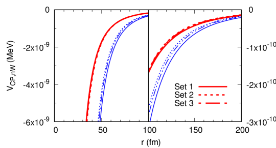
Figure 4: CP-interaction for a neutron and a wall, as a function of the separation distance $r$. Notation is the same as Fig. 2.

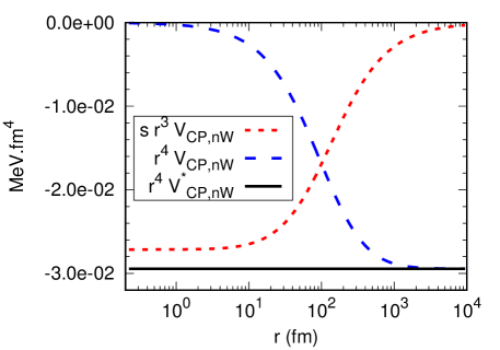
Figure 5: CP-interaction for a neutron and a wall, as a function of the separation distance $r$, multiplied by $s\,r^{3}$ (red dotted line, with $s=100$ fm) and $r^{4}$ (blue long-dashed line). The black solid line is the CP-potential from the static limit of the dipole polarizabilities, multiplied by $r^{4}$.

Figs. 4 and 5 show the CP-interaction for a neutron and a wall, as a function of the separation distance $r$. All the qualitative discussion presented for the CP-interaction between two neutrons also applies here. Notice that in Fig. 5 the factors multiplying $V_{CP,nW}$ are $r^{3}$ and $r^{4}$. The only additional comment is that $V_{CP,nW}$ reaches the expected asymptotic behavior slightly faster than $V_{CP,nn}$, most likely due to the smaller degree of the polynomial $Q(x)$ compared to $P_{E,M}(x)$ multiplying the polarizabilities, see, respectively, Eqs. (IV) and (II).

For very low energy neutrons, in the ultracold region $E_{n}\approx$ several hundreds of neV, the attractive CP interaction would compete with the repulsive Fermi pseudo potential which is given by $V_{F}=\frac{2\pi\hbar^{2}}{M}\rho a$, where $\rho$ is the number density of the atoms in the wall and $a$ is the scattering length of the neutron-nucleus system. The value of $V_{F}$ depends on the material of the wall. E.g. for Ni, $V_{F}$ = 252 neV. Accordingly, for neutron energies below this value, there is an overall repulsion from the wall. In the presence of the CP attractive interaction this situation could potentially change.

The final result, which we consider relevant for this work, is the case of a neutron between two walls. The result is known for neutral atoms and we merely extend it to neutrons. Consider two walls separated by a distance $L$ and a neutron at a distance $z$ from the midpoint within the confines of the two walls $(-L/2\leq z\leq+L/2)$. The confined neutron is subjected to a potential whose form for any value of $L$ is known khar97 ,

$$V_{CP,WnW}(z,L) =-\frac{1}{\pi L^{3}}\int_{0}^{\infty}dt\frac{t^{2}\cosh{(2tz/L)}}{\sinh{(t)}}\int_{0}^{\frac{t}{\alpha_{0}L}}d\omega\alpha(i\omega)$$

$$+\frac{\alpha_{0}^{2}}{\pi L}\int_{0}^{\infty}d\omega\omega^{2}\alpha(i\omega)\int_{\alpha_{0}L\omega}^{\infty}dt\frac{e^{-t}}{\sinh{(t)}}$$

$$=-\frac{1}{\alpha_{0}\pi L^{4}}\int_{0}^{\infty}u^{3}du\,\alpha\left(i\frac{u}{\alpha_{0}L}\right)\int_{1}^{\infty}\frac{dv}{\sinh(uv)}\left[v^{2}\cosh\left(\frac{2z}{L}uv\right)-e^{-uv}\right]$$ (29)

where the latter form is most suitable for numerical calculations, as well as deriving analytic results for specific limits. In particular, if one takes the static limit of Eq. (8) the integrals above can be done exactly, leading to

$$V_{CP,WnW}^{*}(z,L) =-\frac{\alpha_{n}(0)}{\alpha_{0}\pi L^{4}}\left\{\frac{3}{8}\left[\zeta\left(4,\frac{1-f}{2}\right)+\zeta\left(4,\frac{1-f}{2}\right)\right]-\frac{\zeta(4,1)}{4}\right\}$$

$$=-\frac{\pi^{3}\alpha_{n}(0)}{\alpha_{0}L^{4}}\left[\frac{3-2\cos^{2}(\pi f/2)}{8\cos^{4}(\pi f/2)}-\frac{1}{360}\right],$$ (30)

where $f=2z/L$ and

$$\zeta(a,b)=\sum_{k=0}^{\infty}\frac{1}{(k+b)^{a}}$$ (31)

is the generalized Zeta function. Eq. (30) is nothing but the $L\to\infty$ limit khar97 , explicitly showing its $L^{-4}$ behavior. At the midpoint ($z\to 0$) one has $V_{CP,WnW}(0,L)=-11\pi^{3}\alpha_{n}(0)/(90\alpha_{0}L^{4})$. If the neutron is close to one of the walls, the potential diverges towards negative values.

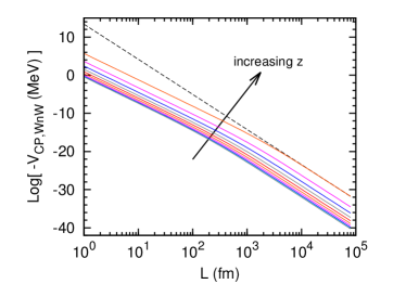
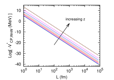
Figure 6: CP-interaction for a neutron between two walls, as a function of the separation $L$. See text for details.

Fig. 6 shows the numerical results of Eq. (29), as functions of the separation $L$ between the walls, for several values of the neutron distance from the midpoint $z$. The lines are for several values of the fraction $f=2z/L$, from 0 to 0.9 in steps of 0.1. The left panel, $V_{CP,WnW}$, shows contributions from the dynamic electric polarizability of the neutron, while the right panel, $V^{*}_{CP,WnW}$, only the static limit. The black dashed line on both panels is the result of Eq. (30) for $f=0.9$ and is drawn just to guide the eye. We can check that the static limit is reached only at distances as large as $\sim 10^{4}$ fm, just a tenth of typical atomic dimensions. This can be better visualized in Fig. 7, with analogously Figs. 3 and 5. Similar to neutron-wall, at small ($\lesssim 10$ fm) and moderate ($\sim 100$ fm) distances the behavior resembles more a $1/L^{3}$ falloff than the asymptotic $1/L^{4}$. The region of this behavior is slightly $z$-dependent, as one compares the the left panel ($f=0.9$) with the right panel ($f=0$) of Fig. 7.

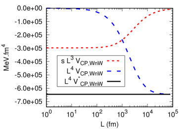
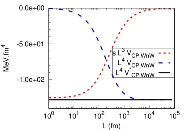
Figure 7: CP-interaction for a neutron between two walls, as a function of the separation $L$ between the walls, multiplied by $s\,L^{3}$ (red dotted line) and $L^{4}$ (blue long-dashed line). The black solid line is the CP-potential from the static limit of the dipole polarizabilities, multiplied by $L^{4}$. Left panel, $z=0.45L$ and $s=1000$ fm. Right panel, $z=0$ fm and $s=200$ fm.

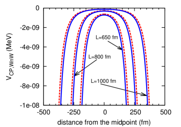
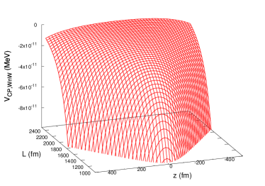
Figure 8: CP-interaction for a neutron between two walls. Left panel, as a function of the neutron position $z$ for three selected values of $L$. Right panel, as a function of both the neutron position $z$ and the separation between the two walls $L$.

In Fig. 8 we present the behavior of $V_{CP,WnW}$ as a function of the neutron distance from the midpoint $z$. On the left panel we select three values of the distance between the walls, $L$, indicated in the figure. The red dashed curves stand for the dynamic polarizability, and the blue solid curves, for the static limit. One sees that the strength of the interaction, as well as the discrepancy of the dynamic and static results, increase as one moves the neutron close to one of the walls. Finally, on the right panel one can inspect the dependence of $V_{CP,WnW}$ on both variables $z$ and $L$, in the region where both the dynamic and static cases are not far from each other.

V Conclusions

In this paper we discussed, derived, and analyzed the dispersive Van der Waals and the retarded dispersive Casimir-Polder interactions between two neutrons and in the proton-neutron system. We found the effect, though very small compared to the by far dominant short range strong interaction, is of significance at large distances, and is stronger in the pn than in the nn system. We further assessed the importance of the low-energy nucleon dynamics, namely, the pion-production threshold and the first excited state of the nucleon, the $\Delta$-resonance (proton (uud), $\Delta^{+}$, $J^{\pi}={3/2}^{+}$, I = 3/2, $I_{z}$ = -1/2; neutron (udd), $\Delta^{0}$, $J^{\pi}={3/2}^{+}$, I = 3/2, $I_{z}$ = +1/2). We found that they dominate the region $\sim 50\,{\rm fm}\lesssim r\lesssim 10^{3}\,{\rm fm}$ in the nn system, the neutron-wall system and in the wall-neutron-wall system. This demonstrates that for $r\gtrsim 50\,{\rm fm}$ the only aspect of the internal quark structure of the nucleon is the induced electric and magnetic dipole moments of the nucleon, a pure dipole stretching of the two down quarks against the up quark in the neutron and the two up quarks against the one down quark in the proton. However, for distances $r\lesssim 50$ fm the studied Casimir-Polder interactions are very sensitive to the electromagnetic response of the short-distance quark-gluon dynamics inside the nucleon. Relevance of our work to confining neutrons inside bottles is briefly discussed.

Our study is exploratory and complementary to the work by Spruch and Kelsey SprKel78 for long-range potentials arising from two-photon exchange in atomic systems. Spruch and Kelsey replaced the static polarizabilities for two atoms appearing in the long-range Casimir-Polder potential by their dynamic polarizabilities. This ansatz was verified rigorously subsequently by two independent Coulomb-gauge quantum electrodynamics calculations BabSpr87 ; Au88 and shown to agree with the dispersion theoretic formalism result FeiSucAu89 . Spruch’s approach is significantly easier to apply than the formal dispersion theoretic analysis and, at least as far as practical calculations, it yields correct long-range interaction potentials. Whether or not this ansatz is good enough or strictly valid for the neutron could be arguable. For example, we note that in their book, Rauch and Werner (Sec. 10.11, p. 313) state that neutrons “…provide the advantage that their Casimir or van der Waals forces are small or perhaps non existing” RauWer15 .

We supposed that the neutron has dynamic electric and magnetic polarizabilities, for which there is certainly evidence from dispersion relations and chiral effective field theory calculations to Compton scattering, and that the neutron interacts as a polarizable particle. Moreover, in using our calculated potentials to model an experiment, other interactions may enter (e.g. the response of the neutron to an applied magnetic field or (as we discussed) perhaps strong interactions). The present work suggests that the topic is deserving of further study and experimental investigations.

VI Acknowledgements

RH appreciates conversations with Vladimir Pascalutsa. JFB is supported in part by the U. S. NSF through a grant for the Institute of Theoretical Atomic, Molecular, and Optical Physics at Harvard University and Smithsonian Astrophysical Observatory. RH and MSH are supported in part by the Fundação de Amparo à Pesquisa do Estado de São Paulo (FAPESP). MSH is also supported by the Conselho Nacional de Desenvolvimento Científico e Tecnológico (CNPq). and by the Coordenação de Aperfeiçoamento de Pessoal de Nível Superior (CAPES), through the CAPES/ITA-PVS program.

References

- (1) J. Schmiedmayer, H. Rauch, and P. Riehs, Nucl. Instrum. Methods A 284, 137 (1989).
- (2) F. Wissmann, M. I. Levchuk, and M. Schumacher, Eur. Phys. J. A 1, 193 (1998).
- (3) H. W. Griesshammer, J. A. McGovern, D. R. Phillips, and G. Feldman, Prog. Part. Nucl. Phys. 67, 841 (2012), arXiv: 1203.6834.
- (4) B. R. Holstein and S. Scherer, Ann. Rev. Nucl. Part. Sci. 64, 51 (2014).
- (5) C. Patrignani et al. (Particle Data Group), Chin. Phys. C, 40, 100001 (2016).
- (6) K. Kossert et al., Eur. Phys. J. A 16, 259 (2003).
- (7) R. M. Thaler, Phys. Rev. 114, 827 (1959).
- (8) J. Schmiedmayer, P. Riehs, J. A. Harvey, and N. W. Hill, Phys. Rev. Lett. 66, 1015 (1991).
- (9) Y. N. Alexandrov, Rev. Mex. Fis. 42, 283 (1996).
- (10) Y. N. Pokotilovski, Eur. Phys. J. A 8, 299 (2000).
- (11) D. Drechsel, B. Pasquini, and M. Vanderhaeghen, Physics Reports 378, 99 (2003).
- (12) F. Hagelstein, R. Miskimen, and V. Pascalutsa, Prog. Part. Nucl. Phys. 88, 29 (2016).
- (13) V. A. Petrunkin, Nucl. Phys. 55, 197 (1964).
- (14) J. J. Karakowski and G. A. Miller, Phys. Rev. C 60, 014001 (1999).
- (15) M. Schumacher, Prog. Part. Nucl. Phys. 55, 567 (2005).
- (16) R. P. Hildebrandt, Ph.D. thesis, Tec. Univ. München, 2005.
- (17) V. Lensky et al., Phys. Rev. C 86, 048201 (2002).
- (18) G. Feinberg and J. Sucher, Phys. Rev. A 2, 2395 (1970).
- (19) G. Feinberg and J. Sucher, Phys. Rev. D 20, 1717 (1979).
- (20) L. G. Arnold, Phys. Lett. B 44, 401 (1973).
- (21) J. Bernabéu and R. Tarrach, Ann. Phys. (N.Y.) 102, 323 (1976).
- (22) J. F. Babb, in Adv. At. Molec. Opt. Phys., edited by E. Arimondo, P. R. Berman, and C. C. Lin (Academic Press, San Diego, 2010), Vol. 59, p. 1.
- (23) L. H. Ford, M. P. Hertzberg, and J. Karouby, Phys. Rev. Lett. 116, 151301 (2016).
- (24) B. R. Holstein, EPJ Web Conf. 134, 01003 (2017).
- (25) R. P. Hildebrandt, H. W. Griesshammer, T. R. Hemmert, and B. Pasquini, Eur. Phys. J. A20, 293 (2004).
- (26) V. Lensky, J. McGovern, and V. Pascalutsa, Eur. Phys. J. C75, 604 (2015).
- (27) M. O’Carroll and J. Sucher, Phys. Rev. 187, 85 (1969).
- (28) H. Friedrich, G. Jacoby, and C. G. Meister, Phys. Rev. A 65, 032902 (2002).
- (29) M. S. Hussein, C. L. Lima, M. P. Pato, and C. A. Bertulani, Phys. Rev. Lett. 65, 839 (1990).
- (30) A. C. C. Villari et al., Phys. Rev. Lett. 71, 2551 (1993).
- (31) G. A. Miller, A. K. Opper and E. J. Stephenson, Ann. Rev. Nucl. Part. Sci. 56, 253 (2006).
- (32) E. Fermi and L. Marshall, Phys. Rev. 71, 666 (1947).
- (33) Y. B. Zeldovich, Zh. Eksp. Teor. Fiz. 36, 1952 (1959) [Sov. Phys. – JETP 9, 1389 (1959)].
- (34) Z.-C. Yan, A. Dalgarno, and J. F. Babb, Phys. Rev. A 55, 2882 (1997)
- (35) P. W. Milonni and M.-L. Shih, Contemp. Phys. 33, 313 (1992).
- (36) H. B. G. Casimir, and D. Polder, Phys. Rev., 73, 360 (1948).
- (37) L. Spruch and E.J. Kelsey, Phys. Rev. A 18, 845 (1978)
- (38) J. F. Babb and L. Spruch, Phys. Rev. A 36, 456 (1987)
- (39) C. K. Au, Phys. Rev. A 38, 7 (1988)
- (40) G. Feinberg, J. Sucher, and C.-K. Au, Phys. Rep. 180, 83 (1989)
- (41) H. Rauch and S. A. Werner, Neutron interferometry : lessons in experimental quantum mechanics, wave-particle duality, and entanglement, (Oxford Univ. Press, Oxford, 2015), second edition, accessed online April 12, 2017.