Lepton asymmetry, neutrino spectral distortions, and big bang nucleosynthesis

Abstract

We calculate Boltzmann neutrino energy transport with self-consistently coupled nuclear reactions through the weak-decoupling-nucleosynthesis epoch in an early universe with significant lepton numbers. We find that the presence of lepton asymmetry enhances processes which give rise to nonthermal neutrino spectral distortions. Our results reveal how asymmetries in energy and entropy density uniquely evolve for different transport processes and neutrino flavors. The enhanced distortions in the neutrino spectra alter the expected big bang nucleosynthesis light element abundance yields relative to those in the standard Fermi-Dirac neutrino distribution cases. These yields, sensitive to the shapes of the neutrino energy spectra, are also sensitive to the phasing of the growth of distortions and entropy flow with time/scale factor. We analyze these issues and speculate on new sensitivity limits of deuterium and helium to lepton number.

I Introduction

In this paper we use the burst neutrino-transport code Grohs et al. (2016) to calculate the baseline effects of out-of-equilibrium neutrino scattering on nucleosynthesis in an early universe with a nonzero lepton number, i.e. an asymmetry in the numbers of neutrinos and antineutrinos. Our baseline includes: a strong, electromagnetic, and weak nuclear reaction network; modifications to the equation of state for the primeval plasma; and a Boltzmann neutrino energy transport network. We do not include neutrino flavor oscillations in this work. Our intent is to provide a coupled Boltzmann transport and nuclear reaction calculation to which future oscillation calculations can be compared. In fact, the outstanding issues in achieving ultimate precision in big bang nucleosynthesis (BBN) simulations will revolve around oscillations and plasma physics effects. These issues exist in both the zero and nonzero lepton-number cases, but are more acute in the presence of an asymmetry.

We self-consistently follow the evolution of the neutrino phase-space occupation numbers through the weak-decoupling-nucleosynthesis epoch. There are many studies of the effects of lepton numbers on light element, BBN abundance yields. Early work Wagoner et al. (1967); Schramm and Wagoner (1977) briefly explored the changes in the helium-4 ($\,{}^{4}\textnormal{He}$) abundance in the presence of large neutrino degeneracies. Later work considered how lepton numbers could influence the $\,{}^{4}\textnormal{He}$ yield Shi (1996); Kirilova and Chizhov (1998) through neutrino oscillations. In addition, other works employed lepton numbers to constrain the cosmic microwave background (CMB) radiation energy density Hansen et al. (2001); Simha and Steigman (2008) or the sum of the light neutrino masses Shiraishi et al. (2009). Refs. Kneller et al. (2001); Mangano et al. (2011) simultaneously investigated BBN abundances and CMB quantities using lepton numbers. The most recent work has used the primordial abundances to constrain lepton numbers which have been invoked to produce sterile neutrinos through matter-enhanced Mikheyev-Smirnow-Wolfenstein (MSW) resonances Abazajian et al. (2005); Smith et al. (2006); Chu and Cirelli (2006). Currently, our best constraints on these lepton numbers come from comparing the observationally-inferred primordial abundances of either $\,{}^{4}\textnormal{He}$ or deuterium (D) with the predicted yields of $\,{}^{4}\textnormal{He}$ and D calculated in these models.

Previous BBN calculations with neutrino asymmetry have made the assumption that the neutrino energy distribution functions have thermal, Fermi-Dirac (FD) shaped forms. In fact, we know that neutrino scattering with electrons, positrons and other neutrinos and electron-positron annihilation produce nonthermal distortions in these energy distributions, with concomitant effects on BBN abundance yields Grohs et al. (2016). Though the nucleosynthesis changes induced with self-consistent transport are small, they nevertheless may be important in the context of high precision cosmology. Anticipated Stage-IV CMB measurements Carlstrom and et al. (2016); Bond et al. (2017) of primordial helium and the relativistic energy density fraction at photon decoupling, coupled with the expected high precision deuterium measurements made with future 30-meter class telescopes Kirkman et al. (2003); Pettini and Cooke (2012); Cooke et al. (2014); Cooke and Pettini (2016); Cooke et al. (2016) will provide new probes of the relic neutrino history.

In the standard cosmology with zero lepton numbers, neutrino oscillations act to interchange the populations of electron neutrinos and antineutrinos ($\nu_{e}$, $\overline{\nu}_{e}$) with those of muon and tau species ($\nu_{\mu}$, $\overline{\nu}_{\mu}$, $\nu_{\tau}$, $\overline{\nu}_{\tau}$) Kostelecký and Samuel (1995). Once we posit that there are asymmetries in the numbers of neutrinos and antineutrinos in one or more neutrino flavors, then neutrino oscillations will largely determine the time and temperature evolution of the neutrino energy and flavor spectra Savage et al. (1991); McKellar and Thomson (1994); Casas et al. (1999); Wong (2002); Abazajian et al. (2002); Dolgov et al. (2002); Gava and Volpe (2010); Johns et al. (2016); Barenboim et al. (2016). In this paper we ignore neutrino oscillations and provide a baseline study of the relationship between neutrino spectral distortions arising from the lengthy ($\sim 10$ Hubble times) neutrino decoupling process and primordial nucleosynthesis. This is an extension of the comprehensive study of this physics in the zero lepton-number case with the burst code Grohs et al. (2016), and in other works Dolgov and Fukugita (1992); Dolgov et al. (1997, 1999); Esposito et al. (2000); Serpico and Raffelt (2005); Mangano et al. (2005); Smith et al. (2008); Saviano et al. (2013); de Salas and Pastor (2016). We will introduce alternative descriptions of the neutrino asymmetry to study the individual processes occurring during weak decoupling. Our studies in this paper, together with the methods in other works, will be important in precision calculations for gauging the effects of flavor oscillations in the early universe.

As we develop below, a key conclusion of a comparison of neutrino-transport effects with and without neutrino asymmetries is nonlinear enhancements of spectral distortion effects on BBN in the former case. This suggests that phenomena like collective oscillations may have interesting BBN effects in full quantum kinetic treatments of neutrino flavor evolution through the weak decoupling epoch.

The outline of this paper is as follows. Section II gives the background analytical treatment of neutrino asymmetry, focusing on the equations germane to the early universe. Sec. III presents the rationale in picking the neutrino-occupation-number binning scheme and other computational parameters. We use the same binning scheme throughout this paper as we investigate how the occupation numbers diverge from FD equilibrium, starting in Sec. IV. In Sec. V, we present a new way of characterizing degenerate neutrinos in the early universe. Sec. VI details the changes to the primordial abundances from the out-of-equilibrium spectra. We give our conclusions in Sec. VII. Throughout this paper we use natural units, $\hbar=c=k_{B}=1$, and assume neutrinos are massless at the temperature scales of interest.

II Analytical Treatment

To characterize the lepton asymmetry residing in the neutrino seas in the early universe, we use the following expression in terms of neutrino, $\nu$, antineutrino, $\overline{\nu}$, and photon, $\gamma$, number densities to define the lepton number for a given neutrino flavor

$$L_{i}\equiv\frac{n_{\nu_{i}}-n_{\overline{\nu}_{i}}}{n_{\gamma}},$$ (1)

where $i=e,\mu,\tau$. The photons are assumed to be in a Planck distribution at plasma temperature $T$, with number density

$$n_{\gamma}=\frac{2\zeta(3)}{\pi^{2}}T^{3},$$ (2)

where $\zeta(3)\approx 1.202$. The neutrino spectra have general nonthermal distributions and their number densities are given by the integration

$$n_{\nu_{i}}=\frac{T_{\textnormal{cm}}^{3}}{2\pi^{2}}\int_{0}^{\infty}d\epsilon\,\epsilon^{2}f_{\nu_{i}}(\epsilon).$$ (3)

Here, $T_{\textnormal{cm}}$ is the comoving temperature parameter and scales inversely with scale factor $a$

$$T_{\textnormal{cm}}(a)=T_{{\rm cm,}i}\left(\frac{a_{i}}{a}\right),$$ (4)

where the $i$ subscripts reflect a choice of an initial epoch to begin the scaling. In this paper, we will choose $T_{{\rm cm,}i}$ such that $T_{\textnormal{cm}}$ is coincident with the plasma temperature when $T=10\,{\rm MeV}$. For $T>T_{{\rm cm,}i}$, the plasma temperature and comoving temperature parameter are nearly equal as the neutrinos are in thermal equilibrium with the photon/electron/positron plasma. $T$ and $T_{\textnormal{cm}}$ diverge from one another once electrons and positrons begin annihilating into photon and neutrino/antineutrino pairs below a temperature scale of $1\,{\rm MeV}$. The dummy variable $\epsilon$ in Eq. (3) is the comoving energy and related to $E_{\nu}$, the neutrino energy, by $\epsilon=E_{\nu}/T_{\textnormal{cm}}$. The sets of $f_{\nu_{i}}$ are the phase-space occupation numbers (also referred to as occupation probabilities) for species $\nu_{i}$ indexed by $\epsilon$. In equilibrium the occupation numbers for neutrinos behave as FD

$$f^{\textnormal{(eq)}}(\epsilon;\xi)=\frac{1}{e^{\epsilon-\xi}+1},$$ (5)

where $\xi$ is the neutrino degeneracy parameter related to the chemical potential as $\xi=\mu/T_{\textnormal{cm}}$. Unlike the lepton number for flavor $i$ in Eq. (1), the corresponding degeneracy parameter $\xi_{i}$ is a comoving invariant. If we consider the equilibrium occupation numbers in the expression for number density, Eq. (3), we find

$$n^{\rm(eq)}_{\nu}=\frac{T_{\textnormal{cm}}^{3}}{2\pi^{2}}\int_{0}^{\infty}d\epsilon\frac{\epsilon^{2}}{e^{\epsilon-\xi}+1}=\frac{T_{\textnormal{cm}}^{3}}{2\pi^{2}}F_{2}(\xi),$$ (6)

where $F_{2}(\xi)$ is the relativistic Fermi integral given by the general expression

$$F_{k}(\xi)=\int_{0}^{\infty}dx\frac{x^{k}}{e^{x-\xi}+1}.$$ (7)

We can define the following normalized number distribution

$$\mathcal{F}(\epsilon;\xi)d\epsilon\equiv\frac{dn}{\int dn}=\frac{1}{F_{2}(\xi)}\frac{\epsilon^{2}d\epsilon}{e^{\epsilon-\xi}+1}.$$ (8)

Figure 1 shows $\mathcal{F}$ plotted against $\epsilon$ for three different values of $\xi$.

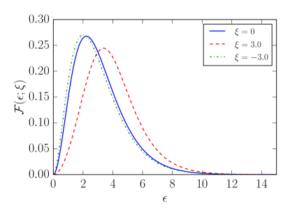
Figure 1: Normalized number density plotted against $\epsilon$ for three choices of degeneracy parameter: nondegenerate ($\xi=0$, solid blue), degenerate with an excess ($\xi=3.0$, dashed red), and degenerate with a deficit ($\xi=-3.0$, dash-dotted green).

The expressions for the number densities in Eqs. (2) and (3) have different temperature/energy scales. As the temperature decreases, electrons and positrons will annihilate to produce photons primarily, thereby changing $T$ with respect to $T_{\textnormal{cm}}$. As a result, Eq. (1) decreases from the addition of extra photons. To alleviate this complication, we calculate the lepton number at a high enough temperature such that the neutrinos are in thermal and chemical equilibrium with the plasma. We can take $T_{\textnormal{cm}}=T$ at high enough temperature and write Eq. (1) as

$$L^{\star}_{i}=\frac{1}{4\zeta(3)}\int_{0}^{\infty}d\epsilon\,\epsilon^{2}[f_{\nu_{i}}(\epsilon)-f_{\overline{\nu}_{i}}(\epsilon)],$$ (9)

where we call $L_{i}^{\star}$ the comoving lepton number. Eq. (9) simplifies further if we use the FD expression in Eq. (5) and recognize that in chemical equilibrium the degeneracy parameters for neutrinos are equal in magnitude and opposite in sign to those of antineutrinos

$$L^{\star}_{i}=\frac{\pi^{3}}{12\zeta(3)}\left[\frac{\xi_{i}}{\pi}+\left(\frac{\xi_{i}}{\pi}\right)^{3}\right],$$ (10)

where $\xi_{i}$ is the degeneracy parameter for neutrinos of flavor $i$. Eq. (10) provides an algebraic expression for relating the lepton number to the degeneracy parameter with no explicit dependence on temperature. We will give our results in terms of comoving lepton number and use Eq. (10) to calculate the degeneracy parameter for input into the computations. In this paper, we will only consider scenarios where all three neutrino flavors have identical comoving lepton numbers. Unless otherwise stated, we will drop the $i$ subscript and replace it with the neutrino symbol, i.e. $L_{\nu}^{\star}$, to refer to all three flavors.

Degeneracy in the neutrino sector increases the total energy density in radiation. The parameter $N_{\textnormal{eff}}$ is defined in terms of the plasma temperature and the radiation energy density

$$\rho_{\rm rad}=\left[2+\frac{7}{4}\left(\frac{4}{11}\right)^{4/3}N_{\textnormal{eff}}\right]\frac{\pi^{2}}{30}T^{4}.$$ (11)

Eq. (11) can be used at any epoch, even one in which there exists seas of electrons and positrons, e.g. Eq. (31) in Ref. Grohs et al. (2016). We will consider $\rho_{\rm rad}$ and $T$ at the epoch $T=1\,{\rm keV}$, after the relic seas of positrons and electrons annihilate. Assuming equilibrium spectra for all neutrino species, the deviation of $N_{\textnormal{eff}}$, $\Delta N_{\textnormal{eff}}$, from exactly 3 would be

$$\Delta N_{\textnormal{eff}}\equiv N_{\textnormal{eff}}-3=\sum\limits_{i}\left[\frac{30}{7}\left(\frac{\xi_{i}}{\pi}\right)^{2}+\frac{15}{7}\left(\frac{\xi_{i}}{\pi}\right)^{4}\right],$$ (12)

where the summation assumes the possibility of different neutrino degeneracy parameters for each flavor Esposito et al. (2000); Shimon et al. (2010).

We begin by presenting the case of instantaneous neutrino decoupling with pure equilibrium FD distributions. Table 1 shows the deviations in energy densities for neutrinos and antineutrinos with respect to nondegenerate FD equilibrium, the asymptotic ratio of $T_{\textnormal{cm}}$ to $T$, and the change to $N_{\textnormal{eff}}$, for various comoving lepton numbers. In this paper, we will colloquially refer to the asymptote of any quantity as the “freeze-out” value. For the values of $L_{\nu}^{\star}$ in Table 1, a decade decrease in $L_{\nu}^{\star}$ produces comparable decreases in $\delta\rho_{\nu}$ and $|\delta\rho_{\overline{\nu}}|$. $L_{\nu}^{\star}$ is related to the energy densities through the degeneracy parameter derived from Eq. (10), which is approximately linear in $\xi$ for small $L_{\nu}^{\star}$. The change in $N_{\textnormal{eff}}$ is quadratic in $\xi$ which is discernible for $L_{\nu}^{\star}=10^{-1}$ and $L_{\nu}^{\star}=10^{-2}$ at the level of precision presented in Table 1. The freeze-out value of $T_{\textnormal{cm}}/T$ is not identically $(4/11)^{1/3}$, the canonical value deduced from covariant entropy conservation Kolb and Turner (1990); Weinberg (2008). Although the neutrino-transport processes are inactive for Table 1 and therefore the covariant entropy is conserved, finite-temperature quantum electrodynamic (QED) effects act to perturb $T_{\textnormal{cm}}/T$ away from the canonical value Heckler (1994); Fornengo et al. (1997).

$L_{\nu}^{\star}$	$\delta\rho_{\nu}$	$\delta\rho_{\overline{\nu}}$	$T_{\textnormal{cm}}/T$	$N_{\textnormal{eff}}$
$10^{-1}$	$0.1485$	$-0.1300$	$0.7149$	$3.0479$
$10^{-2}$	$1.401\times 10^{-2}$	$-1.382\times 10^{-2}$	$0.7149$	$3.0202$
$10^{-3}$	$1.392\times 10^{-3}$	$-1.390\times 10^{-3}$	$0.7149$	$3.0199$
$10^{-4}$	$1.391\times 10^{-4}$	$-1.392\times 10^{-4}$	$0.7149$	$3.0199$
$0$	$0$	$0$	$0.7149$	$3.0199$

Table 1: Observables and related quantities of interest for zero and nonzero comoving lepton numbers without neutrino transport. Column 1 is the comoving lepton number. Columns 2 and 3 give the relative changes of the $\nu$ and and $\overline{\nu}$ energy densities compared to a FD energy distribution with zero degeneracy parameter at freeze-out. Column 4 shows the ratio of comoving temperature parameter to plasma temperature also at freeze-out. For comparison, $(4/11)^{1/3}=0.7138$. Column 5 gives $N_{\textnormal{eff}}$. $N_{\textnormal{eff}}$ does not converge to precisely $3.0$ in the nondegenerate case due to the presence of finite-temperature-QED corrections to the equations of state for photons and electrons/positrons.

III Numerical Approach

For this work, changes to the quantities of interest will be as small as a few parts in $10^{5}$. To ensure our results are not obfuscated by lack of numerical precision, we need an error floor smaller than the numerical significance of a given result. In burst, we bin the neutrino spectra in linear intervals in $\epsilon$-space. The binning scheme has two constraints: the maximum value of $\epsilon$ to set the range; and the number of bins over that range. We denote the two quantities as $\epsilon_{\textnormal{max}}$ and $N_{\textnormal{bins}}$, respectively, and examine how they influence the errors in our procedure.

The mathematical expressions for the neutrino spectra have no finite upper limit in $\epsilon$. We need to ensure $\epsilon_{\textnormal{max}}$ is large enough to encompass the probability in the tails of the curves in Fig. 1. As an example, consider the normalized number density in Eq. (8). We would numerically evaluate the normalization condition as

$$1\simeq\int_{0}^{\epsilon_{\textnormal{max}}}d\epsilon\,\mathcal{F}(\epsilon;\xi).$$ (13)

For large $\epsilon$, $\mathcal{F}\sim\epsilon^{2}e^{-\epsilon+\xi}$, and so we exclude a contribution to the above integral on the order of $\epsilon_{\textnormal{max}}^{2}e^{-\epsilon_{\textnormal{max}}}$ if we take $\xi=0$. If we are using double precision arithmetic, the contribution becomes numerically insignificant for $\mathcal{F}(\epsilon_{\textnormal{max}};0)<10^{-16}$, which corresponds to $\epsilon_{\textnormal{max}}\simeq 44$. This value of $\epsilon_{\textnormal{max}}$ would seem like the natural value to take without loss of a numerically significant contribution to the integral in Eq. (13). However, if we fix the number of abscissa in the partition used when integrating Eq. (13) (i.e. fixing $N_{\textnormal{bins}}$ in the binned neutrino spectra), we lose precision in the evaluation of the contribution to the integral from each bin as we increase $\epsilon_{\textnormal{max}}$. Clearly, there is a trade off between $\epsilon_{\textnormal{max}}$ and $N_{\textnormal{bins}}$.

Figure 2 examines the $\epsilon_{\textnormal{max}}$ versus $N_{\textnormal{bins}}$ parameter space by looking at the calculation of the equilibrium comoving lepton number, in a scenario where $\xi\neq 0$. We take $L_{\nu}^{\star}$ to be exactly $0.1$ and solve the cubic equation in Eq. (10) for $\xi$. Next, we calculate neutrino and antineutrino spectra with the equal and opposite degeneracy parameters. We proceed to integrate Eq. (9) with the two spectra for different pairs of $(N_{\textnormal{bins}},\epsilon_{\textnormal{max}})$ values. The integration is carried out using Boole’s rule, a fifth-order integration method for linearly spaced abscissas. Figure 2 shows the filled contours of $\log_{10}$ values for the error in $L_{\nu}^{\star}$

$$\delta L_{\nu}^{\star}=\biggr{|}\frac{L_{\nu}^{\star}[\epsilon_{\textnormal{max}},N_{\textnormal{bins}}]-0.1}{0.1}\biggr{|},$$ (14)

for a given pair $(N_{\textnormal{bins}},\epsilon_{\textnormal{max}})$. We immediately see the loss of precision in the upper-left corner of the parameter space, corresponding to small $N_{\textnormal{bins}}$ and large $\epsilon_{\textnormal{max}}$. Furthermore, for $\epsilon_{\textnormal{max}}\lesssim 40$, the error value flat lines with increasing $N_{\textnormal{bins}}$, implying that the error is a result of a too small choice for $\epsilon_{\textnormal{max}}$. The black curve superimposed on the heat map gives the value of $\epsilon_{\textnormal{max}}$ with the lowest error as a function of $N_{\textnormal{bins}}$. It monotonically increases for $100<N_{\textnormal{bins}}\lesssim 300$, at which point it reaches $\epsilon_{\textnormal{max}}\sim 40$ and begins to fluctuate. The fluctuations are a result of reaching the double-precision floor, implying that increasing $N_{\textnormal{bins}}$ adds no more numerical significance.

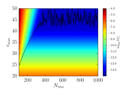
Figure 2: $\epsilon_{\textnormal{max}}$ versus $N_{\textnormal{bins}}$ for contours of constant error in $L_{\nu}^{\star}$. The exact value of $L_{\nu}^{\star}$ is $0.1$. The black line on the contour space gives the value of $\epsilon_{\textnormal{max}}$ with the smallest error as a function of $N_{\textnormal{bins}}$.

The computation time required to run burst scales as $N_{\textnormal{bins}}^{3}$. In this paper, we attempt to be as comprehensive as possible when exploring neutrino energy transport with nonzero lepton numbers. Therefore, we will choose $100$ bins for the sake of expediency. Fig. 2 guides us in picking $\epsilon_{\textnormal{max}}=25$, and dictates a floor of $\sim 10^{-8}$ for our best possible precision. It would appear that the choice $(N_{\textnormal{bins}},\epsilon_{\textnormal{max}})\simeq(300,40)$ would give the absolute best precision for calculating $L_{\nu}^{\star}$. This is valid if using the linearly spaced abscissas as a binning scheme. We highlight both the precision and timing needs for a comprehensive numerical study on binning schemes. Such a study would be germane for the more general problem which includes neutrino oscillations and disparate lepton numbers in the three active species de Salas and Pastor (2016); Barenboim et al. (2016); Johns et al. (2016).

For more details on the numerics of burst, we refer the reader to Ref. Grohs et al. (2016). We have essentially preserved the computational parameters except for a quantity related to the determination of nonzero scattering rates. Ref. Grohs et al. (2016) used $\varepsilon({\rm net}/{\rm FRS})=30$, and in this work, we use $\varepsilon({\rm net}/{\rm FRS})=3$.

IV Neutrino Spectra

In this section we give a detailed accounting of how the neutrino energy spectra evolve through weak decoupling in the presence of zero and nonzero lepton numbers. In the first subsection we integrate the complete transport network, including all the neutrino scattering processes in Table I of Ref. Grohs et al. (2016), from a comoving temperature parameter $T_{\textnormal{cm}}=10\,{\rm MeV}$ down to $T_{\textnormal{cm}}=15\,{\rm keV}$. In the second subsection we investigate how the different interactions between neutrinos and charged leptons affect the spectra.

We compare our results to that of FD equilibrium. For the neutrino occupation numbers, we use the following notation to characterize the deviations from FD equilibrium

$$\delta f_{\xi}(\epsilon)=\frac{f(\epsilon)-f^{\textnormal{(eq)}}(\epsilon;\xi)}{f^{\textnormal{(eq)}}(\epsilon;\xi)}.$$ (15)

Here, $f^{\textnormal{(eq)}}(\epsilon;\xi)$ is the FD equilibrium occupation number for degeneracy parameter $\xi$ given in Eq. (5). When it is obvious, we will drop the argument $\epsilon$, i.e. $\delta f_{\xi}(\epsilon)\rightarrow\delta f_{\xi}$. As an example, $\delta f_{0}$ gives the relative difference of the occupation number from the nondegenerate, zero chemical potential FD equilibrium value.

We also examine the absolute changes for the number and energy distributions

$$\Delta\left(\frac{dn}{d\epsilon}\right)_{\xi}\equiv\frac{T_{\textnormal{cm}}^{3}}{2\pi^{2}}\epsilon^{2}[f(\epsilon)-f^{\textnormal{(eq)}}(\epsilon;\xi)] \quad{\rm(number)},$$ (16)

$$\Delta\left(\frac{d\rho}{d\epsilon}\right)_{\xi}\equiv\frac{T_{\textnormal{cm}}^{4}}{2\pi^{2}}\epsilon^{3}[f(\epsilon)-f^{\textnormal{(eq)}}(\epsilon;\xi)] \quad{\rm(energy)}.$$ (17)

When using the absolute change expressions, we normalize with respect to an equilibrium number or energy density in order to compare to dimensionless expressions. For the energy density, we use the appropriate degeneracy factor

$$\rho_{\xi}\equiv\frac{T_{\textnormal{cm}}^{4}}{2\pi^{2}}\int_{0}^{\infty}d\epsilon\,\epsilon^{3}f^{\textnormal{(eq)}}(\epsilon;\xi).$$ (18)

For the number density, we will exclusively use zero for the degeneracy factor

$$n_{0} \equiv\frac{T_{\textnormal{cm}}^{3}}{2\pi^{2}}\int_{0}^{\infty}d\epsilon\,\epsilon^{3}f^{\textnormal{(eq)}}(\epsilon;0)$$

$$=\frac{3}{4}\frac{\zeta(3)}{\pi^{2}}T_{\textnormal{cm}}^{3}.$$ (19)

The out-of-equilibrium evolution of the neutrino occupation numbers driven by scattering and annihilation processes with charged leptons does not proceed in a unitary fashion. Consequently, the total comoving neutrino number density increases. The increase in number results in an increase in energy density, and so we use $\rho_{\xi}$ to normalize the absolute changes in differential energy density distribution to compare with the initial distribution at high temperature. However, the difference in number density between neutrinos and antineutrinos, characterized by the comoving lepton number in Eq. (9), does not change with kinematic neutrino transport. In practice, burst follows the evolution of neutrino and antineutrino occupation numbers separately, precipitating the possibility of numerical error. We will use the same normalization for neutrino and antineutrino differential number density distributions to study the relative error in $L^{\star}_{i}$. We will take the normalization quantity to be that of the nondegenerate number density in Eq. (19).

IV.1 All processes

Table 2 shows how neutrino transport alters neutrino energy densities, $N_{\textnormal{eff}}$, the ratio of comoving temperature parameter to plasma temperature, and entropy per baryon in the plasma, $s_{\textnormal{pl}}$. These quantities are computed for a range of $L_{i}^{\star}$ values and refer to the results at the end of the transport calculation, $T_{\textnormal{cm}}\sim 1\,{\rm keV}$, well after weak decoupling. In this table, we focus on the energy-derived quantities. The relative changes in energy density are with respect to a nondegenerate FD distribution at the same comoving temperature, i.e.

$$\delta\rho_{i}=\frac{\displaystyle\frac{T_{\textnormal{cm}}^{4}}{2\pi^{2}}\int_{0}^{\infty}d\epsilon\,\epsilon^{3}f_{i}(\epsilon)-\rho_{0}}{\rho_{0}},\quad\rho_{0}=\frac{7}{8}\frac{\pi^{2}}{30}T_{\textnormal{cm}}^{4}.$$ (20)

Columns 2 - 5 of Table 2 show the relative changes in energy density at $T_{\textnormal{cm}}=1\,{\rm keV}$, once the neutrino spectra have converged to their out-of-equilibrium shapes. We see a monotonic decrease in $\delta\rho_{\nu}$ for the neutrinos, and a monotonic increase in $\delta\rho_{\overline{\nu}}$ for the antineutrinos with decreasing $L_{\nu}^{\star}$. Column 6 gives the ratio of $T_{\textnormal{cm}}/T$ at the end of the simulation. $T_{\textnormal{cm}}/T$ increases with decreasing lepton number. However, the decrease is less than one part in $10^{5}$ between $L_{\nu}^{\star}=0.1$ and $L_{\nu}^{\star}=0$. The larger lepton number implies a larger total energy density which increases the Hubble expansion rate. The faster expansion implies a smaller time window for the entropy flow out of the plasma and into the neutrino seas. As a result, the evolution of the plasma temperature is such that larger lepton numbers will maintain $T$ at higher values, and the ratio $T_{\textnormal{cm}}/T$ at freeze-out will decrease, albeit by an amount which is numerically insignificant. With the changes in energy densities and temperature ratios, we can calculate $N_{\textnormal{eff}}$

$$N_{\textnormal{eff}}=\left[\frac{T_{\textnormal{cm}}/T}{(4/11)^{1/3}}\right]^{4}\frac{1}{2}[(2+\delta\rho_{\nu_{e}}+\delta\rho_{\overline{\nu}_{e}})+2(2+\delta\rho_{\nu_{\mu}}+\delta\rho_{\overline{\nu}_{\mu}})].$$ (21)

The coefficient in front of the second parenthetical expression, equal in value to $2$, results from the approximation in taking the $\mu$ and $\tau$ flavors to behave identically. The approximation employed here is valid as there are no $\mu$ and $\tau$ charged leptons in the plasma and $L_{i}$ is the same in all flavors. Both Refs. Mangano et al. (2005); de Salas and Pastor (2016) calculate weak decoupling with a network featuring neutrino flavor oscillations, which are absent in our calculation in Table 2. However, Ref. de Salas and Pastor (2016) states that oscillations have no affect on the value of $N_{\textnormal{eff}}$ at the level of precision which they use. The difference in our value of $N_{\textnormal{eff}}$ versus the standard calculation of Ref. Mangano et al. (2005) is most likely due to a different implementation of the finite-temperature QED effects detailed in Refs. Heckler (1994); Fornengo et al. (1997). Ref. Mangano et al. (2005) uses the perturbative approach outlined in Ref. Mangano et al. (2002) compared to our nonperturbative approach. We leave a detailed study of the finite-temperature-QED-effect numerics to future work.

The final column of Table 2 shows the change in the entropy per baryon in the plasma. The relative changes in entropy for varying lepton numbers are large enough to see a difference at the level of precision Table 2 uses, unlike $T_{\textnormal{cm}}/T$. With the faster expansion, neutrinos have less time to interact with the plasma, yielding a smaller entropy flow.

$L_{\nu}^{\star}$	$\delta\rho_{{\nu_{e}}}$	$\delta\rho_{\overline{\nu}_{e}}$	$\delta\rho_{\nu_{\mu}}$	$\delta\rho_{\overline{\nu}_{\mu}}$	$T_{\textnormal{cm}}/T$	$N_{\textnormal{eff}}$	$10^{3}\times(s_{\textnormal{pl}}^{(i)}/s_{\textnormal{pl}}^{(f)}-1)$
$10^{-1}$	$0.1576$	$-0.1213$	$0.1522$	$-0.1265$	$0.7159$	$3.0800$	$3.809$
$10^{-2}$	$2.298\times 10^{-2}$	$-4.888\times 10^{-3}$	$1.760\times 10^{-2}$	$-1.025\times 10^{-2}$	$0.7159$	$3.0519$	$3.814$
$10^{-3}$	$1.035\times 10^{-2}$	$7.564\times 10^{-3}$	$4.979\times 10^{-3}$	$2.194\times 10^{-3}$	$0.7159$	$3.0516$	$3.815$
$10^{-4}$	$9.096\times 10^{-3}$	$8.817\times 10^{-3}$	$3.725\times 10^{-3}$	$3.446\times 10^{-3}$	$0.7159$	$3.0516$	$3.815$
$0$	$8.957\times 10^{-3}$	$8.957\times 10^{-3}$	$3.585\times 10^{-3}$	$3.585\times 10^{-3}$	$0.7159$	$3.0516$	$3.815$

Table 2: Observables and related quantities of interest in zero and nonzero lepton-number scenarios with neutrino transport. Column 1 is the lepton number. Columns 2, 3, 4, and 5 give the relative changes of the $\nu_{e}$, $\overline{\nu}_{e}$, $\nu_{\mu}$ and $\overline{\nu}_{\mu}$ energy densities compared to a FD energy distribution with zero degeneracy parameter. Comparisons are given for $T_{\textnormal{cm}}\sim 1\,{\rm keV}$, after the conclusion of weak decoupling. Column 6 shows the ratio of comoving temperature parameter to plasma temperature also at the conclusion of weak decoupling. For comparison, $(4/11)^{1/3}=0.7138$. Column 7 gives $N_{\textnormal{eff}}$ as calculated by Eq. (21). Column 8 gives the fractional change in the entropy per baryon in the plasma, $s_{\textnormal{pl}}$.

An increase in lepton number implies a larger energy density for the neutrinos over the antineutrinos. Fig. 3 shows four neutrino spectra after the conclusion of weak decoupling in a scenario where $L_{\nu}^{\star}=0.1$. Plotted against $\epsilon$ is the relative difference in the neutrino occupation number with respect to a nondegenerate spectrum. As seen in the first data row of Table 2, $\delta\rho_{{\nu_{e}}}$ obtains the largest difference from equilibrium. The thick red line in Fig. 3 shows the final out-of-equilibrium spectrum for $\nu_{e}$. The $\nu_{e}$ spectrum has the largest deviation from equilibrium, congruent with Table 2. The black dashed lines show equilibrium spectra for nondegenerate (flat, horizontal line) and degenerate cases. As $\epsilon$ increases, the neutrino curves diverge from the positive $\xi_{\nu}$ spectrum in much the same manner as the antineutrino curves diverge from the negative $\xi_{\overline{\nu}}$. The primary difference in the out-of-equilibrium spectra is due to the initial condition that the neutrinos have larger occupation numbers over the antineutrinos for a positive lepton number.

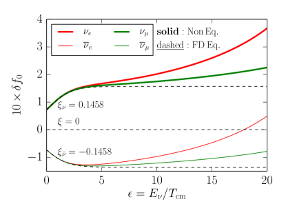
Figure 3: Relative differences in neutrino/antineutrino occupation numbers plotted against $\epsilon$ at $T_{\textnormal{cm}}=1\,{\rm keV}$. The relative differences are with respect to FD with zero degeneracy parameter. The solid lines show the evolution for a scenario where $L_{\nu}^{\star}=0.1$. $\nu_{e}$ and $\overline{\nu}_{e}$ curves are colored red, and $\nu_{\mu}$ and $\overline{\nu}_{\mu}$ curves are colored green. Neutrinos have thick line widths and antineutrinos have thin line widths. Plotted for comparison are black dashed curves representing the equilibrium relative differences. The top dashed curve corresponds to a $\nu$ spectrum with $\xi_{\nu}=0.1458$, the middle horizontal curve corresponds to a $\nu$ spectrum with $\xi_{\nu}=0$, and the bottom dashed curve corresponds to a $\overline{\nu}$ spectrum with $\xi_{\overline{\nu}}=-0.1458$.

We would like to compare the out-of-equilibrium spectra to their respective equilibrium spectra. Such a comparison allows us to examine how the initial asymmetry propagates through the Boltzmann network. Fig. 4 shows the $T_{\textnormal{cm}}$ evolution of $\delta f_{\xi}$ for $\nu_{e}$ (thick solid lines) and $\overline{\nu}_{e}$ (thin solid lines) for a scenario where $L_{\nu}^{\star}=0.1$. We only show the relative differences for three unique values of $\epsilon$, namely $\epsilon=3,\,5,\,7$. The $\nu_{\mu}$ and $\overline{\nu}_{\mu}$ spectra follow similar shapes, but are suppressed relative to the electron flavors. For comparison, we also plot the out-of-equilibrium spectrum for $\nu_{e}$ in the case of no initial asymmetry, i.e. $L_{\nu}^{\star}$ identically zero. It is unnecessary to show the spectrum for $\overline{\nu}_{e}$ when $L_{\nu}^{\star}=0$ because it is exceedingly near the $\nu_{e}$ spectrum (see Fig. [3] of Ref. Grohs et al. (2016)). For the degenerate spectra, the $\overline{\nu}_{e}$ show a larger divergence from equilibrium than the $\nu_{e}$ at these three specific $\epsilon$ values. This is consistent with Ref. Esposito et al. (2000) (see Figs. 8 and 9 therein) and is the case for all $\epsilon$ after the neutrino spectra have frozen out. Fig. 5 shows the final freeze-out values of the relative changes in the neutrino occupation numbers as a function of $\epsilon$. Fig. 5 is similar to Fig. 3 except for the use of the general $\delta f_{\xi}$ instead of $\delta f_{0}$. We have also included the transport-induced out-of-equilibrium spectra for $\nu_{e}$ and $\nu_{\mu}$ in the nondegenerate scenario. For a given flavor, the relative changes in the nondegenerate spectrum are nearly averages of those in the $\nu$ and $\overline{\nu}$ spectra. We also note that for $\epsilon\lesssim 2$, all of the relative differences are negative, although this is obscured in Fig. 5 due to the clustering of lines. For small $\epsilon$, the antineutrino occupation numbers are larger than those of the neutrino, i.e. the $\delta f_{\xi}^{(\overline{\nu})}$ are not as negative.

Figure 4: Relative differences in electron neutrino/antineutrino occupation numbers plotted against $T_{\textnormal{cm}}$. The relative differences are with respect to FD with the same degeneracy parameters as Fig. 3. The solid lines show the evolution for a scenario where $L_{\nu}^{\star}=0.1$. The $\overline{\nu}_{e}$ (thin red curves) has a larger relative change than the $\nu_{e}$ (thick red curves). Plotted for comparison is the relative difference for $\nu_{e}$ in a $L_{\nu}^{\star}=0$ scenario (blue dash-dot curves). The relative differences are plotted for three values of $\epsilon$, from bottom to top: $\epsilon=3,\,5,\,7$.

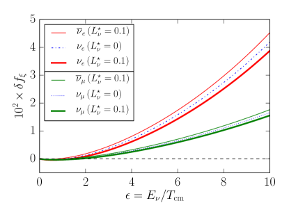
Figure 5: Relative differences in neutrino/antineutrino occupation numbers plotted against $\epsilon$ at $T_{\textnormal{cm}}=1\,{\rm keV}$. The relative differences are with respect to FD with the same corresponding degeneracy parameters as Fig. 3. The solid lines are for a scenario where $L_{\nu}^{\star}=0.1$. Plotted for comparison is the relative difference for $\nu_{e}$ (blue dash-dot curve) and for $\nu_{\mu}$ (blue dotted curve) in a $L_{\nu}^{\star}=0$ scenario.

The weak interaction cross sections scale as $\sigma\sim G_{F}^{2}E^{2}$, where $G_{F}$ is the Fermi constant ($G_{F}\approx 1.166\times 10^{-11}\,{\rm MeV}^{-2}$) and $E$ is the total lepton energy. We would expect a larger difference from equilibrium for increasing $\epsilon$. Except for the range $0<\epsilon\lesssim 1$, Figures 4 and 5 clearly show an increase. The change in the energy distribution does not follow from a scaling relation. Fig. 6 shows the normalized absolute difference in the energy distribution plotted against $\epsilon$ at the conclusion of weak decoupling. The nomenclature for the six lines in Fig. 6 is identical to that of Fig. 5. The energy distributions all show a maximum at $\epsilon\sim 5$. Similar to Fig. 5, the nondegenerate curves of Fig. 6 appear to be averages of the $\nu$ and $\overline{\nu}$ curves in the degenerate scenario.

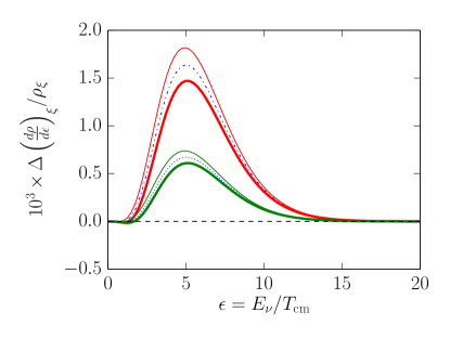
Figure 6: Absolute change in the neutrino/antineutrino energy distributions plotted against $\epsilon$ at $T_{\textnormal{cm}}=1\,{\rm keV}$. The changes are with respect to the same degeneracy parameters as those in Fig. 5. Furthermore, the line colors and styles correspond to the same species and scenarios as Fig. 5.

In the positive lepton-number scenarios, the $\overline{\nu}$ always have larger occupation numbers than the $\nu$, when compared against the equilibrium degenerate spectrum/distribution. This is not surprising as the occupation numbers for antineutrinos are suppressed, implying less blocking. When compared against its equilibrium distribution, the $\overline{\nu}$ have larger rates, leading to a larger distortion. In Fig. 7, we compare the out-of-equilibrium number density distributions with those of the nondegenerate case solely. In other words, the normalizing factor $n_{0}$ is the same for each of the six curves in Fig. 7. We have adopted this nomenclature for the comparison of number density distributions to study the change in the comoving lepton number. None of the weak decoupling processes modify the lepton number in our model. The total change in number density for $\nu$ should be identical to the total change in number density for $\overline{\nu}$. Fig. 7 shows this indirectly. We can see a difference; the $\nu$ curves are skewed to higher $\epsilon$ and have a larger maximum than the $\overline{\nu}$. The negative change in the distributions for the range $0\leq\epsilon\lesssim 2$ is much more noticeable in Fig. 7 than in Fig. 5. It is clear that the changes in $\overline{\nu}$ become positive for smaller $\epsilon$ than those of $\nu$, implying there are more $\overline{\nu}$ than $\nu$ for $\epsilon\lesssim 2$. Overall, when integrating the curves in Fig. 7, the total changes in number density for $\overline{\nu}$ should be the same as for $\nu$. We have calculated this quantity and expressed it as a relative change in the $L_{i}^{\star}$, taken to be exactly $0.1$

$$\delta L_{i}^{\star}\equiv\frac{\displaystyle\frac{1}{4\zeta(3)}\int_{0}^{\infty}d\epsilon\,\epsilon^{2}[f_{\nu_{i}}(\epsilon)-f_{\overline{\nu}_{i}}(\epsilon)]-0.1}{0.1}.$$ (22)

Eq. (22) gives the relative error in our calculation. We conserve the comoving lepton number for both electron and muon flavor at approximately $7\times 10^{-6}$. Also plotted in Fig. 7 are the absolute changes for $\nu_{e}$ and $\nu_{\mu}$ in the nondegenerate scenario. We do not directly compare the lepton-number relative errors as the quantity is not defined for the symmetric case. We do note that the nondegenerate curves are close to the average of the $\nu$ and $\overline{\nu}$ distributions, similar to that of Figs. 5 and 6.

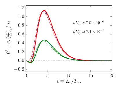
Figure 7: Absolute change in the neutrino/antineutrino number distributions plotted against $\epsilon$ at $T_{\textnormal{cm}}=1.0\,{\rm keV}$. The changes are with respect to the same degeneracy parameters, and the nomenclature of line colors and line styles is the same as those in Fig. 5. The numbers given on the plot ($\delta L_{i}^{\star}$ for $i=e,\mu$) show the relative error accumulated over the course of a simulation.

In Figs. 3 through 7, we have only presented the $L_{\nu}^{\star}=0.1$ scenario. Fig. 8 shows the relative differences in occupation number for $\nu$ plotted against $\epsilon$ for other values of $L_{\nu}^{\star}$. The behavior of each curve is in line with those of Fig. 5. Not plotted are the curves for $\overline{\nu}$. They also behave in a similar manner, where $\delta f_{\overline{\nu}}$ becomes larger than $\delta f_{0}$ for increasing $\epsilon$. The result is that with transport, $L_{\nu}^{\star}$ acts to increase the asymmetries in the occupation numbers, which manifest in differences in the absolute changes of the differential energy density.

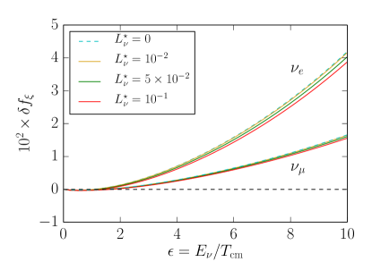
Figure 8: Relative differences in neutrino occupation numbers plotted against $\epsilon$ at $T_{\textnormal{cm}}=1\,{\rm keV}$ for various values of $L_{\nu}^{\star}$. The relative differences are with respect to FD with the corresponding degeneracy parameter, namely $\xi=0.1458$ ($L_{\nu}^{\star}=10^{-1}$), $\xi=0.0730$ ($L_{\nu}^{\star}=5\times 10^{-2}$), $\xi=0.0146$ ($L_{\nu}^{\star}=10^{-2}$), and $\xi=0$ ($L_{\nu}^{\star}=0$). Shown are two sets of curves: the set with the larger relative differences correspond to the $\nu_{e}$ spectral distortions, and the set with the smaller differences are $\nu_{\mu}$. Within each set, the increase in $L_{\nu}^{\star}$ leads to a decrease in $\delta f_{\xi}$. For the antineutrinos, the relative differences behave in the opposite manner: increase in $L_{\nu}^{\star}$ leads to an increase in $\delta f_{\xi}$.

IV.2 Individual processes

Figs. 5 and 6 demonstrate that the initial asymmetry in the neutrino energy density is maintained and even amplified by scattering processes. We can dissect the relative contribution of various scattering processes to this amplification.

Figs. 9 and 10 show the absolute changes in the number density distribution versus $\epsilon$ when we include only certain transport processes. Fig. 9 contains three annihilation processes, schematically shown as:

$$\nu_{i}+\overline{\nu}_{i}\leftrightarrow e^{-}+e^{+},\quad i=e,\mu,\tau.$$ (23)

In this scenario, we have included only the annihilation channel into electron/positron pairs when computing transport. The changes are with respect to the same degeneracy parameters as those in Fig. 5. The line colors in Fig. 9 correspond to the same species as Fig. 5. Because of the close proximity of the neutrino and antineutrino curves, we depart from the previous nomenclature of emphasizing the $\nu$ curves with a thicker line width so as not to obscure the $\overline{\nu}$ curves. For this plot, the absolute differences are normalized with respect to the equilibrium number density at temperature $T_{\textnormal{cm}}$ with degeneracy parameter $\xi=0$. For a given neutrino species, the total change in number density should be equal to the change in number density for the corresponding antineutrino.

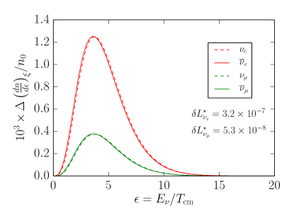
Figure 9: Absolute change in the neutrino/antineutrino number distributions plotted against $\epsilon$ at $T_{\textnormal{cm}}=1.0\,{\rm keV}$. The numbers given on the plot ($\delta L_{i}^{\star}$ for $i=e,\mu$) show the relative error accumulated over the course of a simulation.

Fig. 10 shows the effect of including 12 elastic scattering processes:

$$\nu_{i}+e^{-} \leftrightarrow\nu_{i}+e^{-},$$ (24)

$$\nu_{i}+e^{+} \leftrightarrow\nu_{i}+e^{+},$$ (25)

and the opposite-$CP$ reactions, for neutrino flavors $i=e,\mu,\tau$. In this scenario, we have included only the elastic scattering channel with electrons/positrons (while neglecting the neutrino-antineutrino only channels) when computing transport. The changes are with respect to the same degeneracy parameters as those in Fig. 5. Furthermore, the line colors and styles in Fig. 10 correspond to the same species and scenarios as Fig. 5. For this plot, the absolute differences are normalized with respect to the equilibrium number density at temperature $T_{\textnormal{cm}}$ with degeneracy parameter $\xi=0$. In an identical manner to the processes in Fig. 9, the total change in $\nu$ number density should be equal to the change in number density for the corresponding $\overline{\nu}$ in Fig. 10.

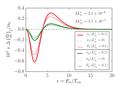
Figure 10: Absolute change in the neutrino/antineutrino number distributions plotted against $\epsilon$ at $T_{\textnormal{cm}}=1.0\,{\rm keV}$. The numbers given on the plot ($\delta L_{i}^{\star}$ for $i=e,\mu$) show the relative error accumulated over the course of a simulation.

The elastic scattering processes of Eqs. (24) and (25) (and the opposite-$CP$ reactions) preserve the total number of neutrinos and antineutrinos. The plasma of charged leptons acts to upscatter low energy neutrinos and antineutrinos to higher energies, precipitating an entropy flow. Fig. 10 vividly shows a deficit of neutrinos in the range $0<\epsilon\lesssim 4$, and the corresponding excess for $\epsilon\gtrsim 4$. The deficit is more pronounced in Fig. 10 but also appeared in Figs. 5, 6, and 7 when computing the entire neutrino-transport network. The annihilation processes, shown in Fig. 9, do not preserve the total numbers of neutrinos and antineutrinos and can fill the phase space vacated by the upscattered neutrinos. The complete transport network, which includes annihilation, elastic scattering on charged leptons, and elastic scattering among only neutrinos/antineutrinos, is able to redistribute the added energy by filling the occupation numbers for lower epsilon.

V Integrated asymmetry measures

In our presentation to this point, we have used the comoving lepton number to describe the asymmetry in the early universe. $L_{i}^{\star}$ does not evolve with temperature in our model, except for errors in precision encountered by our code. Therefore, we introduce two integrated quantities to examine how the initial asymmetry propagates to later times. The quantities provide new means to analyze the out-of-equilibrium spectra.

The first integrated quantity we define is the lepton energy density asymmetry

$$R_{i}\equiv\frac{\rho_{\nu_{i}}-\rho_{\overline{\nu}_{i}}}{\frac{\pi^{2}}{15}T_{\textnormal{cm}}^{4}}.$$ (26)

where $i$ is the flavor index. Like the comoving lepton number in Eq. (9), we divide Eq. (26) by $T_{\textnormal{cm}}^{4}$ so that $R_{i}$ is comoving and dimensionless. This will allow us to follow the evolution of $R_{i}$ to later times. At large $T_{\textnormal{cm}}$, all flavors have identical equilibrium FD spectra and lepton numbers/degeneracy parameters. For degeneracy parameter $\xi$, we calculate the equilibrium value of $R$

$$R^{\rm(eq)}={\rm sgn}(\xi)\left[\vphantom{\frac{7}{8}}\right. \frac{7}{8}+\frac{15}{4}\left(\frac{\xi}{\pi}\right)^{2}+\frac{15}{8}\left(\frac{\xi}{\pi}\right)^{4}$$

$$- \left.\frac{90}{\pi^{4}}e^{-|\xi|}\Phi(-e^{-|\xi|},4,1)\right],$$ (27)

where ${\rm sgn}(x)$ is the sign function with real-number argument $x$, and $\Phi(z,s,v)$ is the Lerch function (see Sec. 9.55 of Ref. Gradshteyn and Ryzhik (2007))

$$\Phi(z,s,v)\equiv\sum\limits_{n=0}^{\infty}\frac{z^{n}}{(n+v)^{s}};\,|z|<1;\,v\neq 0,-1,-2,....$$ (28)

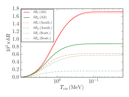
Figure 11: The relative changes in $R$ plotted against $T_{\textnormal{cm}}$ for $\nu_{e}$ and $\nu_{\mu}$ with different processes included in the transport calculation. Red lines correspond to $\nu_{e}$ and green lines correspond to $\nu_{\mu}$. The process scheme is all processes (solid curves), annihilation only (dash-dot curves), or elastic scattering only (dotted curves).

Figure 11 shows the relative changes in $R_{i}$ from the $R^{\rm(eq)}$ baseline ($\delta R_{i}$), plotted against $T_{\textnormal{cm}}$ for different combinations of transport processes. Solid lines (All) are for the complete calculation, whereas dash-dot curves only include the annihilation channels (Annih.) of the reaction shown in (23), and dotted curves only include the elastic scattering channels (Scatt.) of the reactions shown in (24), (25), and the opposite-$CP$ reactions. Red lines correspond to $\delta R_{e}$ and green lines to $\delta R_{\mu}$. $\delta R_{i}$ increases for all six combinations of flavor and transport process, until an eventual freeze-out. Indirectly, Figs. 7, 9, and 10 all show that the neutrinos have larger changes in the energy density distributions, increasing the asymmetry. Because of the charged-current process, $\delta R_{e}$ experiences a greater enhancement. What is important to note is that the total $\delta R_{i}$, for either flavor, is not an incoherent sum of the two transport processes taken individually. There are two reasons for this.

First, there are other transport processes in the full calculation. Neutrinos scattering on other neutrinos and antineutrinos will redistribute energy density. Second, the transport processes with the charged leptons are dependent on one another. Positron-electron annihilation into neutrino-antineutrino pairs populates the lower energy levels. Those particles upscatter on charged leptons through elastic scattering. Positron-electron annihilation is then suppressed by the Pauli blocking of the upscattered particles. Both reasons change the evolution of the total $R_{i}$, but do so in a flavor-dependent manner. For $\delta R_{\mu}$, the incoherent sum of annihilation and elastic scattering is smaller than that of the total asymmetry. For $\delta R_{e}$, the total asymmetry is dominated by the contribution from elastic scattering.

In analogy with the lepton energy density asymmetry, we define the lepton entropy asymmetry as

$$\Sigma_{i}\equiv\frac{S_{\nu_{i}}-S_{\overline{\nu}_{i}}}{\frac{4}{3}\frac{\pi^{2}}{15}T_{\textnormal{cm}}^{3}}$$ (29)

where $S_{j}$ is the entropic density for particle $j$, given by

$$S_{j}=-\frac{T_{\textnormal{cm}}^{3}}{2\pi^{2}}\int_{0}^{\infty}d\epsilon\,\epsilon^{2}[f_{j}\ln f_{j}+(1-f_{j})\ln(1-f_{j})],$$ (30)

and we have suppressed the arguments of $f_{j}(\epsilon;\xi)$ for brevity in notation. Under the equilibrium assumptions, we find

$$\Sigma^{\rm(eq)}=R^{\rm(eq)}-\frac{45}{2\pi^{4}}\xi\left[\zeta(3)|L^{\star}_{\nu}|+e^{-|\xi|}\Phi(-e^{-|\xi|},3,1)\right].$$ (31)

Fig. 12 shows the evolution of the relative change in $\Sigma_{i}$ away from $\Sigma^{\rm(eq)}$ when divided into processes. The nomenclature for the line styles and colors is identical to that in Fig. 11. The evolution of the lepton entropy asymmetry shows more features than that of the lepton energy density asymmetry.

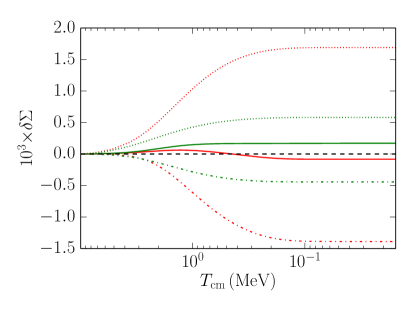
Figure 12: The relative changes in $\Sigma$ plotted against $T_{\textnormal{cm}}$. Line colors and styles correspond to the same transport processes and neutrino flavors in Fig. 11.

To understand the dynamics of $\Sigma_{i}$ in Fig. 12, we begin by considering how the entropy depends on perturbations to the occupation numbers. We write the occupation numbers as differences from FD equilibrium

$$f_{j}(\epsilon;\xi)=f^{\textnormal{(eq)}}_{j}(\epsilon;\xi)+\Delta f_{j}(\epsilon;\xi).$$ (32)

We can calculate the change in the entropy produced by the out-of-equilibrium occupation numbers by substituting Eq. (32) into Eq. (30). After dropping the $\epsilon$ argument, $\xi$ argument, and species index for notational brevity, we find for small $\Delta f$

$$S =-\frac{T_{\textnormal{cm}}^{3}}{2\pi^{2}}\int_{0}^{\infty}d\epsilon\,\epsilon^{2}[(f^{\textnormal{(eq)}}+\Delta f)\ln(f^{\textnormal{(eq)}}+\Delta f)+(1-f^{\textnormal{(eq)}}-\Delta f)\ln(1-f^{\textnormal{(eq)}}-\Delta f)]$$ (33)

$$\simeq-\frac{T_{\textnormal{cm}}^{3}}{2\pi^{2}}\int_{0}^{\infty}d\epsilon\,\epsilon^{2}\left[f^{\textnormal{(eq)}}\ln f^{\textnormal{(eq)}}+(1-f^{\textnormal{(eq)}})\ln(1-f^{\textnormal{(eq)}})+\Delta f\ln\frac{f^{\textnormal{(eq)}}}{1-f^{\textnormal{(eq)}}}\right]$$ (34)

$$=S^{\rm(eq)}-\frac{T_{\textnormal{cm}}^{3}}{2\pi^{2}}\int_{0}^{\infty}d\epsilon\,\epsilon^{2}\Delta f[\xi-\epsilon]$$ (35)

$$=S^{\rm(eq)}-\xi\Delta n+\Delta\rho/T_{\textnormal{cm}},$$ (36)

where $\Delta n$ and $\Delta\rho$ are the changes in number and energy density, respectively, from equilibrium. The expression for the lepton entropy asymmetry is

$$\Sigma_{i}=\Sigma^{\rm(eq)}+\frac{45}{4\pi^{2}T_{\textnormal{cm}}^{3}}\left[-\xi(\Delta n_{\nu_{i}}+\Delta n_{\overline{\nu}_{i}})+\frac{\Delta\rho_{\nu_{i}}-\Delta\rho_{\overline{\nu}_{i}}}{T_{\textnormal{cm}}}\right].$$ (37)

Lepton number is conserved in our scenarios, implying $\Delta n_{\nu_{i}}=\Delta n_{\overline{\nu}_{i}}$. As a result, we can write the lepton entropy asymmetry as

$$\Sigma_{i}=\Sigma^{\rm(eq)}+\frac{45}{4\pi^{2}T_{\textnormal{cm}}^{3}}\left[-2\xi\Delta n_{\nu_{i}}+\frac{\Delta\rho_{\nu_{i}}-\Delta\rho_{\overline{\nu}_{i}}}{T_{\textnormal{cm}}}\right].$$ (38)

Eq. (38) shows how the lepton entropy asymmetry changes for small perturbations to the occupation numbers. Two trends are evident from this equation. First, adding particles ($\Delta n_{\nu_{i}}>0$) decreases the asymmetry. Second, increasing the asymmetry in energy density ($\Delta\rho_{\nu_{i}}-\Delta\rho_{\overline{\nu}_{i}}>0$), leads to an increase in the lepton entropy asymmetry. For the annihilation processes, the changes in the number density distribution for neutrinos and antineutrinos vary in the same way across $\epsilon$ space for all flavors (see Fig. 9). Therefore, the corresponding changes in the energy density will also be the same, and there will be no contribution to the change in $\Sigma$ from the energy density terms. The dash-dot curves in Fig. 12 shows the relative change in $\Sigma$ for a run with only the annihilation channels active. Both the $e$ and $\mu$ flavors show a suppression in $\Sigma$ with decreasing $T_{\textnormal{cm}}$. Figure 10 shows that for elastic scattering of neutrinos and charged leptons, the neutrino and antineutrino number density distributions are not coincident. Overall, each neutrino species has zero net change in number density, as elastic scattering can only redistribute the number. Therefore, there will be no contribution to the change in $\Sigma$ from the number density term. As there are more neutrinos over antineutrinos for $L_{\nu}^{\star}>0$, elastic scattering enhances the neutrino spectra over the antineutrino spectra. The result is a net positive change in the energy density differences. Fig. 12 shows an increase in the relative change in $\Sigma$ for the elastic-scattering-only runs for both flavors. When we add the elastic-scattering and annihilation channels together, along with the other transport processes which do not involve charged leptons, we see that the two processes essentially cancel, leaving only a modest change in $\Sigma_{i}$ as shown by the solid lines in Fig. 12.

Figure 13: Same as Fig. 12 except zoomed in on the solid curves.

The interesting thing to note in Fig. 12 is the asymmetry between flavors. Fig. 13 is a zoomed-in version of the solid lines in Fig. 12. We see that $\delta\Sigma_{\mu}$ is monotonically increasing for decreasing $T_{\textnormal{cm}}$. The incoherent sum of the relative changes from the annihilation and elastic-scattering processes in Fig. 12 nearly gives the relative change in $\Sigma_{\mu}$ that we obtain when all transport processes are active. The same cannot be said for $\delta\Sigma_{e}$. The sum of the two transport processes is not incoherent, the evolution of $\delta\Sigma_{e}$ is not monotonic, and the final freeze-out value of $\delta\Sigma_{e}$ is of opposite sign from $\delta\Sigma_{\mu}$. Although the elastic scattering would appear to produce a larger enhancement of $\delta\Sigma_{e}$ over the suppression of annihilation, the two processes do not have equal weight. We observe this by looking at the maxima in the number density distributions in Figs. 9 and 10. The ratio of maxima in Fig. 9 for annihilation is

$$\left(\frac{dn_{{\nu_{e}}}}{d\epsilon}\right)\biggr{/}\left(\frac{dn_{\nu_{\mu}}}{d\epsilon}\right)\simeq 3.5\quad{\rm(Annih.)}$$ (39)

The ratio of maxima in Fig. 10 for elastic scattering is

$$\left(\frac{dn_{{\nu_{e}}}}{d\epsilon}\right)\biggr{/}\left(\frac{dn_{\nu_{\mu}}}{d\epsilon}\right)\simeq 3.0\quad{\rm(Scatt.)}$$ (40)

This shows that annihilation is more dominant in the electron neutrino/antineutrino sector than it is in the $\mu$ sector. In Figs. 9 and 10, we have only showed the final distributions at freeze-out. Electron-positron annihilation into neutrinos is not always so dominant, as evidenced by the positive values of $\Sigma_{e}$ for $T_{\textnormal{cm}}\gtrsim 400\,{\rm keV}$.

The analysis of the lepton entropy asymmetry focused on the transport processes which involve the charged leptons. The other scattering processes redistribute occupation number and therefore change $\Sigma_{i}$. However, we have verified that the contributions from the transport processes which involve only neutrinos or antineutrinos do not alter $\Sigma_{i}$ enough to explain the full evolution shown in Fig. 13. The transport processes which involve the charged leptons play the dominant roles.

We have considered the evolution of the integrated asymmetry measures for $L_{\nu}^{\star}=0.1$ only. Table 3 gives the relative changes in $R_{i}$ and $\Sigma_{i}$ at freeze-out for various values of $L_{\nu}^{\star}$. Note that the positive relative changes for $L_{\nu}^{\star}<0$ imply an absolute decrease in either quantity. We see that the differences between the various values of $L_{\nu}^{\star}$ are beneath the error floor.

$L_{\nu}^{\star}$	$10^{4}\times\delta R_{e}$	$10^{4}\times\delta R_{\mu}$	$10^{4}\times\delta\Sigma_{e}$	$10^{4}\times\delta\Sigma_{\mu}$
$10^{-1}$	$17.20$	$8.802$	$-0.8211$	$1.714$
$10^{-2}$	$17.26$	$8.825$	$-0.8804$	$1.692$
$10^{-3}$	$17.27$	$8.828$	$-0.8729$	$1.694$
$-10^{-1}$	$17.20$	$8.802$	$-0.8214$	$1.714$
$-10^{-2}$	$17.26$	$8.825$	$-0.8820$	$1.691$
$-10^{-3}$	$17.24$	$8.828$	$-0.9001$	$1.694$

Table 3: Relative changes in integrated asymmetry measures at freeze-out for select values of comoving lepton number $L_{\nu}^{\star}$.

VI Abundances

Our calculations show potentially significant changes in lepton-asymmetric BBN abundance yields with neutrino transport relative to those without. With the inclusion of transport we find that the general trends of the yields of $\,{}^{4}\textnormal{He}$ and D with increasing or decreasing lepton number are preserved: positive $L_{\nu}^{\star}$ decreasing the yields of both, while negative lepton numbers increase both. In broad brush, Boltzmann transport makes little difference for helium, but gives a $\geq 0.3\%$ reduction in the offset from the FD, zero lepton-number case with transport. This change in the reduction is comparable to uncertainties in BBN calculations arising from nuclear cross sections and from plasma physics and QED issues. For all BBN calculations, the baryon to photon ratio is fixed to be $n_{b}/n_{\gamma}=6.0747\times 10^{-10}$ (equivalent to the baryon density $\omega_{b}=0.022068$ given by Ref. Planck Collaboration et al. (2014)). In addition, the mean neutron lifetime is taken to be $885.7\,{\rm s}$.

Table 4 contains relative differences in the primordial abundances with and without transport. Columns with the label “FD Eq.” are the calculations without any active transport processes. The spectra freeze-out at high temperatures where they are in FD equilibrium with a degeneracy parameter corresponding to $L_{\nu}^{\star}$. Columns with the label “Boltz.” are the calculations in the full Boltzmann neutrino-transport calculation. Relative differences are with respect to the appropriate abundance in the zero-degeneracy Boltz. calculation. The relative changes in the abundances for the two different calculations are quite close: $\delta Y_{P}$ differs by 2 - 3 parts in $10^{4}$; and $\delta{\rm D/H}$ differs by 3 - 4 parts in $10^{3}$. Both differences are consistent across $L_{\nu}^{\star}$. We caution against any interpretation that links the two calculations together, as the No Trans. calculations ignore important physics related to non-FD spectra, entropy flow, and the Hubble expansion rate.

We have examined the detailed evolution of the spectra and integrated asymmetry measures in the Boltz. calculations. The electron neutrinos and antineutrinos behave differently compared to muon and tau flavored neutrinos. This behavior will have ramifications for the neutron-to-proton ratio and nucleosynthesis. To facilitate the analysis of the effects of neutrino transport on BBN, we will introduce a model which uses additional radiation energy density. We will try to determine whether this simplistic “dark radiation” model Grohs et al. (2015); Mukohyama (2000) – which includes radiation energy density distinct from photons and active neutrinos, but does not include transport – can mock up the effects of the extra energy density which arise from neutrino scattering and the associated spectral distortions. We will compare this dark-radiation model to the full neutrino-transport case. For ease in notation when comparing the two scenarios, we will abbreviate the dark-radiation model as “DR” and the full Boltzmann neutrino-transport calculation as Boltz.

$L_{\nu}^{\star}$	$\delta Y_{P}$ (FD Eq.)	$\delta Y_{P}$ (Boltz.)	$\delta({\rm D/H})$ (FD Eq.)	$\delta({\rm D/H})$ (Boltz.)
$10^{-1}$	$-0.1333$	$-0.1331$	$-6.972\times 10^{-2}$	$-6.654\times 10^{-2}$
$10^{-2}$	$-1.425\times 10^{-2}$	$-1.400\times 10^{-2}$	$-1.101\times 10^{-2}$	$-7.618\times 10^{-3}$
$10^{-3}$	$-1.678\times 10^{-3}$	$-1.409\times 10^{-3}$	$-4.206\times 10^{-3}$	$-7.815\times 10^{-4}$
$7.139\times 10^{-3}$	$-1.027\times 10^{-2}$	$-1.001\times 10^{-2}$	$-8.867\times 10^{-3}$	$-5.463\times 10^{-3}$
$1.364\times 10^{-2}$	$-1.931\times 10^{-2}$	$-1.906\times 10^{-2}$	$-1.371\times 10^{-2}$	$-1.033\times 10^{-2}$
$-10^{-1}$	$0.1475$	$0.1479$	$8.566\times 10^{-2}$	$8.947\times 10^{-2}$
$-10^{-2}$	$1.384\times 10^{-2}$	$1.415\times 10^{-2}$	$4.352\times 10^{-3}$	$7.825\times 10^{-3}$
$-10^{-3}$	$1.133\times 10^{-3}$	$1.407\times 10^{-3}$	$-2.669\times 10^{-3}$	$7.630\times 10^{-4}$
$-7.071\times 10^{-3}$	$9.692\times 10^{-3}$	$9.968\times 10^{-3}$	$2.047\times 10^{-3}$	$5.495\times 10^{-3}$
$-1.240\times 10^{-2}$	$1.724\times 10^{-2}$	$1.756\times 10^{-2}$	$6.253\times 10^{-3}$	$9.740\times 10^{-3}$

Table 4: Relative changes in primordial abundances of ${}^{4}{\rm He}$ and D in two calculations of BBN with nonzero comoving lepton numbers $L_{\nu}^{\star}$. FD Eq. signifies the calculation without transport. Boltz. signifies the full Boltzmann neutrino-transport network calculation. The abundances are given as relative changes from the zero degeneracy, full Boltzmann calculation. Column 1 is the comoving lepton number. Column 2 gives the relative change of $Y_{P}$ at freeze-out in the no-transport model. Column 3 gives the relative change of $Y_{P}$ at freeze-out in the Boltz. calculation. The relative changes for D/H are given in columns 4 and 5. The four rows where $|L_{\nu}^{\star}|$ is not a power of 10 are projected sensitivity limits for $1\%$ changes in the primordial abundances.

In the DR model, we introduce extra radiation energy density, $\rho_{\rm dr}$, described at early times by the dark-radiation parameter $\delta_{\textnormal{dr}}$

$$\rho_{\rm dr}=\frac{7}{8}\frac{\pi^{2}}{15}\delta_{\textnormal{dr}}T_{\textnormal{cm}}^{4}.$$ (41)

The FD Eq. calculation in Table 4 used $\delta_{\textnormal{dr}}=0$. We mandate that the dark radiation be composed of relativistic particles which are not active neutrinos. We have chosen the specific form of Eq. (41) for conformity with $N_{\textnormal{eff}}$, namely $\Delta N_{\textnormal{eff}}\approx\delta_{\textnormal{dr}}$. The relation is not a strict equality due to the presence of finite-temperature-QED corrections to the electron rest mass Grohs et al. (2016); Heckler (1994); Fornengo et al. (1997); Cambier et al. (1982); Lopez and Turner (1999). The DR model differs from the Boltz. calculation in multiple respects. First, the DR model fixes the neutrino spectra to be in degenerate FD equilibrium. Second, neutrino transport induces an entropy flow from the plasma into the neutrino seas, absent in the DR model. Third, the entropy flow changes the phasing of the plasma temperature with the comoving temperature parameter as compared to the case of instantaneous neutrino decoupling in the DR model. The phasing is dependent on the Hubble expansion rate and the flow of entropy. Although the expansion rates are identical in the two scenarios, the entropy flows are not.

For all calculations, we will fix $\delta_{\textnormal{dr}}=0.03149$. We pick this specific value to match $N_{\textnormal{eff}}$ between the DR model and Boltz. calculation for the single case $L_{\nu}^{\star}=0.1$. The change in $N_{\textnormal{eff}}$ depends on the Hubble expansion rate, which depends on the initial degeneracy. Therefore, our choice of $\delta_{\textnormal{dr}}$ will not ensure equal values of $N_{\textnormal{eff}}$ between the two scenarios for $L_{\nu}^{\star}\neq 0.1$. Although our DR model is not consistent across all $L_{\nu}^{\star}$, the changes in $N_{\textnormal{eff}}$ are small for the range of $L_{\nu}^{\star}$ we explored.

Figure 14 shows the relative changes in abundances versus the comoving lepton number for both calculations. Our baselines for comparison are the abundances in the nondegenerate case, $L_{\nu}^{\star}=0$, from the Boltz. calculation. As a result of the choice of baseline, the relative changes in abundances for the DR model will not converge to zero as $L_{\nu}^{\star}\rightarrow 0$. We use a mass fraction to describe the helium abundance, $Y_{P}$, and relative abundances with respect to hydrogen to describe deuterium (D), helium-3 (${}^{3}{\rm He}$), and lithium-7 (${}^{7}{\rm Li}$). The solid lines in Fig. 14 show the relative changes in the DR model. Positive relative changes in the abundances correspond to negative comoving lepton numbers, and negative changes to positive $L_{\nu}^{\star}$. We also show individual points using the Boltz. calculation at three decades of $L_{\nu}^{\star}$, namely $\log_{10}|L_{\nu}^{\star}|=-1,-2,-3$. Squares correspond to $L_{\nu}^{\star}>0$, and circles to $L_{\nu}^{\star}<0$.

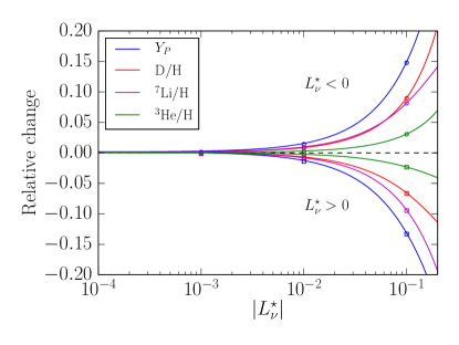
Figure 14: Relative changes in the primordial abundances plotted against the absolute value of the comoving lepton number. Positive changes in abundances correspond to negative comoving lepton numbers, and negative changes correspond to positive comoving lepton numbers. The solid lines use the dark-radiation model described in the text. Individual points using the full Boltzmann-transport calculation are plotted for three decades of $L_{\nu}^{\star}$. Squares correspond to $L_{\nu}^{\star}>0$, and circles for $L_{\nu}^{\star}<0$. The baryon density is fixed to be $\omega_{b}=0.022068$ (equivalent to a baryon-to-photon ratio $n_{b}/n_{\gamma}=6.0747\times 10^{-10}$) for all calculations in both scenarios Planck Collaboration et al. (2014). . The mean neutron lifetime is taken to be $885.7\,{\rm s}$.

All abundances decrease with increasing $L_{\nu}^{\star}$. A nonzero comoving lepton number changes the occupation numbers in the neutron-proton interconversion rates, and also changes the Hubble expansion rate. The neutron-to-proton ratio ($n/p$) is sensitive to both quantities Smith et al. (2009); Grohs and Fuller (2016), and $Y_{P}$ is the abundance most sensitive to $n/p$. In Fig. 14, we see that $Y_{P}$ has the largest change from the nondegenerate baseline, while ${}^{3}\textnormal{He}$ has the least sensitivity to $L_{\nu}^{\star}$. Deuterium and ${}^{7}\textnormal{Li}$ have a more intricate relationship with $L_{\nu}^{\star}$. As we increase $L_{\nu}^{\star}$ from large negative values towards zero, we see that the relative change for D is larger than that for ${}^{7}\textnormal{Li}$ until $L_{\nu}^{\star}\sim-5\times 10^{-2}$. At this point, ${}^{7}\textnormal{Li}$ appears to be more sensitive to $L_{\nu}^{\star}$. The trend continues for $L_{\nu}^{\star}>0$, as the relative change in ${}^{7}\textnormal{Li}$ is more negative than that of D. The asymmetry between $L_{\nu}^{\star}>0$ and $L_{\nu}^{\star}<0$ in the relative changes of D and ${}^{7}\textnormal{Li}$ is present in $Y_{P}$ and ${}^{3}\textnormal{He}$ also. With the exception of ${}^{7}\textnormal{Li}$, all abundances are more sensitive to negative $L_{\nu}^{\star}$. All trends occur in both the DR model and Boltz. calculation. These trends are similar but have minor differences than those discussed in Ref. Kneller and Steigman (2004).

Table 5 gives the relative changes of $Y_{P}$ and D/H for various values of $L_{\nu}^{\star}$ in both scenarios. Columns with the label “(DR)” are relative changes calculated with the dark-radiation model and columns with the label “(Boltz.)” are relative changes in the full Boltzmann neutrino-transport calculation. The Boltz. columns in Table 5 are identical to the Boltz. columns in Table 4. For all four abundance columns, the relative changes are with respect to the abundance calculated with the full Boltzmann-transport network with degeneracy parameter set to zero, consistent with the lines and points in Fig. 14. For the Boltz. columns, the relative changes in $Y_{P}$ tend to be twice as large as those in D/H. Each decade change in $L_{\nu}^{\star}$ induces close to a decade change in both relative abundances. We have included calculations for sets of lepton numbers which aim for $\pm 1\%$ changes in both $Y_{P}$ and D/H in the Boltz. calculation. For the DR model, the relative changes for $\,{}^{4}\textnormal{He}$ and deuterium are in line with the Boltz. calculation for $L_{\nu}^{\star}=+0.1$. Transport enhances the $\nu_{e}$ occupation numbers over the $\overline{\nu}_{e}$ if $L_{\nu}^{\star}=+0.1$. The extra probability in the $\nu_{e}$ spectrum enhances the rate of ${\nu_{e}}+n\rightarrow p+e^{-}$. As a result, the helium abundance decreases further in the Boltz. calculation, which is evident in Table 5. Conversely, for $L_{\nu}^{\star}=-0.1$, transport will enhance the $\overline{\nu}_{e}$ over the $\nu_{e}$ and we would expect an increase in the $\,{}^{4}\textnormal{He}$ abundance. This is not the case in Table 5 - the DR model has a larger $\delta Y_{P}$ than the Boltz. calculation.

$L_{\nu}^{\star}$	$\delta Y_{P}$ (DR)	$\delta Y_{P}$ (Boltz.)	$\delta{\rm(D/H)}$ (DR)	$\delta{\rm(D/H)}$ (Boltz.)
$10^{-1}$	$-0.1318$	$-0.1331$	$-6.589\times 10^{-2}$	$-6.654\times 10^{-2}$
$10^{-2}$	$-1.257\times 10^{-2}$	$-1.400\times 10^{-2}$	$-6.823\times 10^{-3}$	$-7.618\times 10^{-3}$
$10^{-3}$	$2.683\times 10^{-5}$	$-1.409\times 10^{-3}$	$2.054\times 10^{-5}$	$-7.815\times 10^{-4}$
$7.139\times 10^{-3}$	$-8.576\times 10^{-3}$	$-1.001\times 10^{-2}$	$-4.467\times 10^{-3}$	$-5.463\times 10^{-3}$
$1.364\times 10^{-2}$	$-1.762\times 10^{-2}$	$-1.906\times 10^{-2}$	$-9.540\times 10^{-3}$	$-1.033\times 10^{-2}$
$-10^{-1}$	$0.1494$	$0.1479$	$9.038\times 10^{-2}$	$8.947\times 10^{-2}$
$-10^{-2}$	$1.556\times 10^{-2}$	$1.415\times 10^{-2}$	$8.627\times 10^{-3}$	$7.825\times 10^{-3}$
$-10^{-3}$	$2.840\times 10^{-3}$	$1.407\times 10^{-3}$	$1.566\times 10^{-3}$	$7.630\times 10^{-4}$
$-7.071\times 10^{-3}$	$1.141\times 10^{-2}$	$9.968\times 10^{-3}$	$6.309\times 10^{-3}$	$5.495\times 10^{-3}$
$-1.240\times 10^{-2}$	$1.897\times 10^{-2}$	$1.756\times 10^{-2}$	$1.054\times 10^{-2}$	$9.740\times 10^{-3}$

Table 5: Relative changes in primordial abundances of ${}^{4}{\rm He}$ and D in two calculations of neutrino transport with nonzero comoving lepton numbers $L_{\nu}^{\star}$. DR signifies the dark-radiation model of neutrino transport and Boltz. signifies the full Boltzmann neutrino-transport network calculation. The columns are the same as Table 4 with the replacement of “FD Eq.” by DR.

The error in the above logic resides in the treatment of the rate which changes protons to neutrons, namely $\overline{\nu}_{e}+p\rightarrow n+e^{+}$. This reaction has a threshold of $Q\equiv\delta m_{np}+m_{e}\simeq 1.8\,{\rm MeV}$, where $\delta m_{np}$ and $m_{e}$ are the neutron-to-proton mass difference and electron rest mass, respectively. If we define the appropriate $\epsilon$-value for $Q$ to be $q\equiv Q/T_{\textnormal{cm}}$, we can see where and how the threshold plays a role in $\epsilon$ and $T_{\textnormal{cm}}$ space. Fig. 7 shows the freeze-out distortion to the differential number density distributions for $L_{\nu}^{\star}=+0.1$. The $\nu_{e}$ and $\overline{\nu}_{e}$ spectra would be switched if we had plotted $L_{\nu}^{\star}=-0.1$, i.e. a “mirror” of Fig. 7. At the start of the calculation at $T_{\textnormal{cm}}=10\,{\rm MeV}$, the distortions are identically zero. The calculation proceeds and the peaks in $\Delta(dn/d\epsilon)$ for $\nu_{e}$ and $\overline{\nu}_{e}$ grow. The locations of the peaks do change with decreasing $T_{\textnormal{cm}}$, but we have verified that the shift in position is small compared to peak location of $\epsilon\sim 4$. We claimed above that the extra number density of $\overline{\nu}_{e}$ over $\nu_{e}$ would increase the rate $\overline{\nu}_{e}+p\rightarrow n+e^{+}$, but it is only the number density with $\epsilon$-value larger than $q$ which is able to increase the rate, thereby decreasing the neutron abundance. At $T_{\textnormal{cm}}=1\,{\rm MeV}$, $q\simeq 2$ which is large enough to exclude a portion of the left-hand side of the peak, effectively limiting the number of antineutrinos which could participate in the channel $\overline{\nu}_{e}+p\rightarrow n+e^{+}$. At $T_{\textnormal{cm}}=500\,{\rm keV}$, $q\simeq 4$ which is nearly coincident with the central location of the peak. This is the point in $T_{\textnormal{cm}}$ where the $\,{}^{4}\textnormal{He}$ abundance begins to depart from nuclear statistical equilibrium Smith et al. (1993). Although the abundance is $\sim 15$ orders of magnitude smaller than its freeze-out value, the integration of the nuclear reaction network is sensitive to the initial conditions, and already half of the peak width in the mirror of Fig. 7 is unavailable to enhance the rate and modify the neutron-to-proton ratio. The formation of $\,{}^{4}\textnormal{He}$ nuclei is typically ascribed to the epoch $T_{\textnormal{cm}}=100\,{\rm keV}$, where $q\simeq 20$ and well larger than the range where the distortions in the mirror of Fig. 7 could affect the rate for $\overline{\nu}_{e}+p\rightarrow n+e^{+}$. Meanwhile, neutrino transport is inducing an increased population on the high-energy tail of the $\nu_{e}$ spectrum, which would increase the neutron to proton rate ${\nu_{e}}+n\rightarrow p+e^{-}$. This reaction has no threshold, and so the entire peak in the mirror of Fig. 7, integrated over the full range of $T_{\textnormal{cm}}$, would increase the rate. Incidentally, $e^{+}+n\rightarrow p+\overline{\nu}_{e}$ has no threshold and this process is also important in setting $n/p$. However, in this case, the spectral distortion effects we described above would tend to hinder this process by producing extra $\overline{\nu}_{e}$ blocking. The $\overline{\nu}_{e}$ in $e^{+}+n\rightarrow p+\overline{\nu}_{e}$ has a minimum energy of $Q$, and so the expected suppression of this rate from additional $\overline{\nu}_{e}$ number density suffers from the same sequence of events as mentioned above.

To summarize, transport-induced $\nu_{e}$ and $\overline{\nu}_{e}$ spectral distortions develop over such a long time span that the threshold-limited $\overline{\nu}_{e}$ number density cannot overcome the $\nu_{e}$ number density when calculating the neutron-proton interconversion rates in the $L_{\nu}^{\star}=-0.1$ case. The result is a decrease in $\delta Y_{P}$ for the Boltz. calculation compared to the DR model.

The DR model is tuned to have the same total energy density as produced in the full Boltzmann calculation when $L_{\nu}^{\star}=\pm 0.1$. If $|L_{\nu}^{\star}|\neq 0.1$, the radiation energy density, and by extension $N_{\textnormal{eff}}$, is slightly different. The abundances are sensitive to the change in $N_{\textnormal{eff}}$, and as a result we see significant differences between the two models in Table 5. An especially egregious example is the $L_{\nu}^{\star}=10^{-3}$ scenario, where the relative changes in $\,{}^{4}\textnormal{He}$ are 2 orders of magnitude different and have different signs. We conclude that mocking up the effect of neutrino transport in this model with dark radiation fails for small lepton numbers. However, if we had tuned the DR model for $N_{\textnormal{eff}}$ to agree when $L_{\nu}^{\star}=10^{-3}$, we would have had better agreement for smaller $L_{\nu}^{\star}$. We note that for all cases with $|L_{\nu}^{\star}|\leq 7\times 10^{-3}$, the changes in the abundances are below current and projected error tolerances Carlstrom and et al. (2016).

VII Conclusion

We have done the first nonzero neutrino chemical potential calculations of weak decoupling and BBN with full Boltzmann neutrino transport simultaneously coupled with all relevant strong, weak, and electromagnetic nuclear reactions. We have performed these calculations with a modified version of the burst code. This code and the physics it incorporates is described in detail in Ref. Grohs et al. (2016). By design, our calculations here do not include neutrino flavor oscillations. Our intent was to provide baseline calculations for comparison to future neutrino flavor quantum kinetic treatments (see Refs. Barbieri and Dolgov (1991); Volpe et al. (2013) in the early universe, and Refs. Raffelt and Sigl (1993); Balantekin and Pehlivan (2007); Volpe (2015) in core-collapse supernova cores, for a discussion on the quantum kinetic equations in their respective environments). One objective of this baseline Boltzmann study was to identify how a significant lepton number would affect out-of-equilibrium neutrino scattering and the concomitant neutrino scattering-induced flow of entropy out of the photon-electron-positron plasma and into the decoupling neutrino component. A related objective was to assess whether (and how) the scattering-induced neutrino spectral distortions develop differently in the case of a significant neutrino asymmetry. The third objective was to use a new description to connect the two previously mentioned phenomena: macroscopic thermodynamics of entropy flow, and microscopic spectral distortions. Finally, the last objective was to assess the impact of these neutrino spectral distortions and the accompanying changes in entropy flow and temperature/scale factor phasing on BBN light element abundance yields. A key finding of our full Boltzmann neutrino-transport treatment is that the presence of a lepton-number asymmetry enhances the processes which give rise to distortions from equilibrium, FD-shaped neutrino and antineutrino energy spectra. Our transport calculations show a positive feedback between out-of-equilibrium neutrino scattering and any initial distortion from a zero chemical potential FD distribution (see the elastic scattering of neutrinos with charged leptons in Fig. 10). An initial distortion, for example, stemming from a nonzero chemical potential, is amplified by neutrino scattering, at least for higher values of the comoving neutrino energy parameter $\epsilon=E_{\nu}/T_{\textnormal{cm}}$. Of course, overall lepton asymmetry is preserved by the nonlepton number violating scattering processes we treat here.

In broad brush, as the Universe expands entropy is transferred from the electron-positron component into photons, with neutrinos receiving only a small portion of this entropy largess. The magnitude of this small entropy increase to the decoupling neutrinos is governed largely by the out-of-equilibrium scattering of neutrinos and antineutrinos on the electrons and positrons, which are generally “hotter” than the neutrinos. The neutrino scattering cross sections scale like $\sigma\sim\epsilon^{2}$, and therefore higher energy neutrinos are able to extract entropy from the photon-electron-positron component more effectively than neutrinos with lower energy. The result is that a “bump” or occupation excess (see Fig. 7) on the higher energy end of the neutrino energy distribution function grows with time. Our transport calculations have allowed us to track both entropy flow between the neutrinos and the plasma and the simultaneous development of neutrino spectral distortions, all for a range of initial lepton asymmetries. For the larger values of lepton asymmetry considered here we found that the entropy transferred to neutrinos is decreased by a few tenths of a percent over the zero lepton-number case (see Table 2).

The enhanced neutrino spectral distortions and entropy transfer revealed by our full Boltzmann-transport calculations might be expected to translate into corresponding nuclear abundance changes emerging from BBN. Our full coupling between neutrino scattering and the weak interaction sector and the nuclear reaction network is uniquely adapted to treat this physics. Indeed, for the zero neutrino chemical potential cases, the full Boltzmann-neutrino transport resulted in a deuterium BBN yield $\sim 1\,\%$ different than a calculation with no neutrino transport and a sharp weak decoupling approximation (see Table V of Ref. Grohs et al. (2016)). The baseline Boltzmann transport calculations with significant lepton asymmetries reported here show that the shift in BBN abundances with nonzero neutrino chemical potentials are closely in line with those reported in sharp weak decoupling studies Kneller and Steigman (2004), but with a few peculiarities. The enhanced spectral distortions discussed above for the lepton asymmetry cases do alter the charged-current weak interaction neutron-to-proton interconversion rates and, in turn, this leads to altered abundance yields over the no-transport, sharp decoupling treatment. To put these alterations in perspective, our full Boltzmann calculations of BBN show that the $\,{}^{4}\textnormal{He}$ abundance yield is sensitive at the one percent level to an initial, comoving lepton number of $L_{\nu}^{\star}\approx 7\times{10}^{-3}$, while the deuterium abundance yield is similarly sensitive to $L_{\nu}^{\star}\approx 1.5\times{10}^{-2}$. This is significant because the next generation CMB experiments, e.g. proposed Stage-4 CMB observations Carlstrom and et al. (2016), target precisions for independent primordial helium abundance determinations at roughly the two percent level. Likewise, the next generation of large optical telescopes, for example 30-meter class telescopes Silva et al. (2007); Skidmore et al. (2015); McCarthy and Bernstein (2014); Hook (2005) (ed.), are touted as providing a comparable level of precision in determining the primordial deuterium abundance from quasar absorption lines in high redshift damped Lyman-alpha systems. Our calculations show that we would need $\sim 0.1\,\%$ precision in these primordial abundance determinations to probe different treatments of neutrino scattering in the weak decoupling epoch, at least for the case with no neutrino oscillations.

Though our calculations show that the bulk of the alteration in abundances stems from the initial lepton asymmetry itself, transport does produce offsets in absolute abundances yields comparable to those with zero lepton numbers. We found that sometimes we can adequately capture the BBN effects of full Boltzmann neutrino transport by using a dark radiation model of extra radiation energy density added by neutrino scattering. However, this approximation, tuned to agree with the Boltzmann calculation results at one value of comoving lepton number, fails for other lepton asymmetry values.

We showed in Table 5 how neutrino transport alters the primordial abundances in degenerate cases. Both $\,{}^{4}\textnormal{He}$ and D are sensitive to $n/p$, which itself is sensitive to the $\nu_{e}$ and $\overline{\nu}_{e}$ occupation numbers. Table 4 showed that the FD Eq. treatment of BBN closely matches the Boltz. calculation of $Y_{P}$. Transport induces a relative change in D/H nearly an order or magnitude larger than that of $Y_{P}$. This finding is consistent with findings in the zero-degeneracy case Grohs et al. (2016). Tables 2 and 5 show that the primordial abundances are more sensitive to neutrino degeneracy than $N_{\textnormal{eff}}$. Moreover, $\,{}^{4}\textnormal{He}$ is twice as sensitive to the degeneracy than D. CMB Stage-IV experiments Carlstrom and et al. (2016); Abazajian and et al. (2015) and 30-meter-class telescopes will probe $Y_{P}$, D/H, and $N_{\textnormal{eff}}$ at the $1\%$ level. If future observations were to find little change in $N_{\textnormal{eff}}$ from the standard prediction, but changes in the abundances matching the patterns in Table 5, then this scenario would be consistent with a degeneracy in the neutrino sector. However, the Boltz. calculations in Table 5 do not include the physics of neutrino oscillations. In the presence of nonzero lepton numbers, oscillations may alter the scaling relations of Table 5 and will necessitate a full quantum kinetic equation treatment Vlasenko et al. (2014); Blaschke and Cirigliano (2016).

This brings us to the question of our selection of initial lepton asymmetries. We have chosen to examine values of these at and below usually accepted limits, and we have examined only situations where the asymmetries are the same across all flavors. The trends our Boltzmann-transport calculations reveal will likely hold for lepton asymmetries outside of the ranges considered here. However, differences in lepton numbers between different flavors will drive medium-enhanced/affected neutrino flavor transformation which could lead to different conclusions in the neutrino sector. Comparing future quantum kinetic calculations which include both coherent and scattering-induced flavor transformation with our strict Boltzmann treatment might reveal BBN and $N_{\textnormal{eff}}$ signatures of neutrino flavor conversion, although these may be at levels well below what future observations and experiments can probe.

Nevertheless, many beyond-standard-model physics considerations invoke quite small initial lepton numbers Harvey and Turner (1990); Kawasaki et al. (2002); Bezrukov et al. (2010); Merle et al. (2014). Various models of sterile neutrinos in the early universe, including dark matter models, rely on lepton number-driven medium enhancements Shi and Fuller (1999); Abazajian et al. (2001); Kishimoto et al. (2006) or beyond-standard-model physics to create relic sterile-neutrino densities (see Refs. de Gouvea and et al. (2013); Adhikari and et al. (2016) and references therein for a review of sterile neutrino dark matter). Sterile neutrinos are an intriguing dark matter candidate Dodelson and Widrow (1994), and could conceivably be congruent with particle Kusenko et al. (2010) and cosmological bounds Yamaguchi (2003); Abazajian (2014). For resonantly produced sterile neutrino dark matter, the models invoke lepton asymmetries in the ${10}^{-3}$ to ${10}^{-5}$ range to match the relic dark-matter abundance, providing a motivation for our choice of values for $L_{\nu}^{\star}$.

In fact, many models for baryon and lepton-number generation in the early universe March-Russell et al. (1999); Gu (2010); Canetti et al. (2013) , e.g. the neutrino minimal standard model ($\nu$MSM) Asaka et al. (2005); Shaposhnikov and Tkachev (2006) , can produce lepton numbers in the ranges chosen for the the present study. It will be interesting to see if future quantum kinetic calculations with neutrino flavor transformation will yield deviations from the baseline calculations presented here. Any such deviations would point to either a different distribution of lepton numbers over neutrino flavor than that considered here, or differences in the development of scattering-induced spectral distortions and attendant BBN abundance alterations over the standard scenario.