Probing QCD perturbation theory at high energies
with continuum extrapolated lattice data

Abstract

Precision tests of QCD perturbation theory are not readily available from experimental data. The main reasons are systematic uncertainties due to the confinement of quarks and gluons, as well as kinematical constraints which limit the accessible energy scales. We here show how continuum extrapolated lattice data may overcome such problems and provide excellent probes of renormalized perturbation theory. This work corresponds to an essential step in the ALPHA collaboration’s project to determine the $\Lambda$-parameter in 3-flavour QCD. I explain the basic techniques used in the high energy regime, namely the use of mass-independent renormalization schemes for the QCD coupling constant in a finite Euclidean space time volume. When combined with finite size techniques this allows one to iteratively step up the energy scale by factors of 2, thereby quickly covering two orders of magnitude in scale. We may then compare perturbation theory (with $\beta$-functions available up to 3-loop order) to our non-perturbative data for a 1-parameter family of running couplings. We conclude that a target precision of 3 percent for the $\Lambda$-parameter requires non-perturbative data up to scales where $\alpha_{s}\approx 0.1$, whereas the apparent precision obtained from applying perturbation theory around $\alpha_{s}\approx 0.2$ can be misleading. This should be taken as a general warning to practitioners of QCD perturbation theory.

1 Introduction

Lattice QCD is usually thought of as a tool to extract non-perturbative information about QCD in the hadronic regime. Therefore it is widely believed that lattice QCD is limited to the low energy regime where the cutoff (i.e. the inverse lattice spacing, $1/a$) sets the limit for accessible scales, typically at a few ${\rm GeV}$. In this talk I would like to dispel this myth and draw the wider QCD community’s attention to the fact that lattice QCD provides excellent ways to probe perturbation theory at high energies and indeed covering a range of energy scales orders of magnitude apart (cf. Brida:2016flw and references therein). To understand the origin of the above mentioned misconception we first need to remind ourselves that hadronic physics is done in physically large volumes such that the linear extent of the volume, $L$, is large in units of the Compton-wave length of the pion, $1/m_{\pi}$, which is the lightest particle around. At least for single particle states, the infinite volume limit is reached exponentially fast Luscher:1985dn and, depending on the target precision and the particular observables under study, it may be sufficient to require $m_{\pi}L>4$ for sub-percent errors Aoki:2013ldr . With typical lattice spacings in the range $0.04$ - $0.1$ ${\rm fm}$, and for pion masses close to physical this implies lattice sizes up to $L/a=128$. This is at the limit of current technical feasibility and there is thus no room to further reduce the lattice spacing without compromising in some other way.

So how can this limitation be overcome? It starts with the simple observation that perturbation theory can be applied to observables defined in a smaller volume than is required for hadronic physics. Finite volume effects are then not dominated by pion physics and might still be under control for the perturbative observables under study. One may take this a step further by making the finite volume a part of the definition of the perturbative observable Jansen:1995ck . In this case there is no need to extrapolate to infinite volume and one may freely move up and down the energy scale, thus reaching high energies of O(100) ${\rm GeV}$. The main drawback is that the finiteness of the volume becomes a defining property of the observable, so that perturbation theory must be done in finite volume, too. Depending on the chosen boundary conditions this may substantially enhance the technical difficulties of perturbation theory.

2 How to probe the accuracy of perturbation theory

Observables in QCD are defined in terms of renormalized correlation functions of gauge invariant composite fields via the QCD path integral,

$$\left\langle O\right\rangle={\cal Z}^{-1}\int D[A,\psi,\bar{\psi}]\,O[A,\psi,\bar{\psi}]\exp\left(-S\right)\,,$$ (1)

where $A_{\mu}$, $\psi$ and $\bar{\psi}$ denote the gluon, quark and anti-quark fields and we have here assumed the Euclidean framework. Many such correlation functions have a well-defined perturbative expansions in powers of a renormalized coupling, $\alpha_{s}(\mu)=\bar{g}^{2}(\mu)/4\pi$,

$$\left\langle O\right\rangle=c_{0}+c_{1}\alpha_{s}(\mu)+c_{2}\alpha_{s}^{2}(\mu)+\ldots,$$ (2)

where the renormalization scale $\mu$ is a priori arbitrary. However, the perturbative series behaves best if $\mu$ is chosen close to the relevant physical scales involved in the correlation function, given typically by particle masses, energies or momenta. Moreover, for the perturbative description to become accurate, $\mu$ must be in the “perturbative regime", $\mu\gg\Lambda$, where the $\Lambda$-parameter is around a few hundred ${\rm MeV}$ in the $\overline{\rm MS}$ scheme. How can a statement about the accuracy of perturbation theory be made more quantitative? Besides non-perturbative data, obtained either from experiment or from the lattice, one would like to have several orders of the perturbative series available. However, due to the asymptotic nature of the series it is probably even more important to vary the size of the expansion parameter, $\alpha_{s}(\mu)$, which is tantamount to varying the scale $\mu$.

For observables defined as in eqs. (1,2) one may normalize the perturbative expansion by defining an “effective coupling", through

$$\alpha_{O}(\mu)=\dfrac{\left\langle O\right\rangle-c_{0}}{c_{1}}=\alpha_{s}(\mu)+c_{1}^{\prime}\alpha_{s}^{2}(\mu)+c_{2}^{\prime}\alpha_{s}^{3}(\mu)+\ldots,$$ (3)

so that its expansion starts with $\alpha_{s}(\mu)$. In principle, $\alpha_{O}(\mu)$ can be derived from an experimentally measured observable. However, some practical problems tend to limit the accuracy:

1. While perturbation theory takes the path integral as starting point, its non-perturbative connection to the experimental observable requires some assumption about the transition from quark and gluon to hadronic degrees of freedom. The root of the problem is confinement of quarks in hadrons, an inherently non-perturbative phenomenon.

2. The scale $\mu$ is usually constrained by the kinematics of the experiment under consideration. For example in $\tau$-decays, $\mu$ is essentially determined by the $\tau$-lepton’s mass Pich:2016bdg ; Boito:2016oam . It is then not possible to vary the energy scale and the only control over the perturbative expansion is obtained by studying the apparent convergence of the asymptotic series.

3. For observables defined at energies of a few GeV, the dependence of the effective coupling on the charm and bottom quark masses cannot be ignored so that one uses effective theories with $N_{\rm f}=3,4,5$ quark flavours, perturbatively matched at the charm and bottom thresholds.

None of these limitations applies to non-perturbative lattice data in physically small volumes. Numerical simulations provide non-perturbative estimates of the Euclidean path integral which can be directly compared to the perturbative saddle point expansion. The up, down and strange quark masses can be set to zero and the heavier quarks omitted, thereby “switching off" the charm and bottom thresholds. As a result the effective coupling becomes a non-perturbatively defined running coupling in a quark mass independent renormalization scheme Weinberg:1951ss for 3-flavour QCD, and its scale dependence can be traced over a range of scales several orders of magnitude apart.

3 A family of finite volume couplings

An attractive class of finite volume couplings can be obtained by imposing Dirichlet boundary conditions on the fields at Euclidean times $x_{0}=0$ and $x_{0}=T$. Due to its relation with the Schrödinger representation in Quantum Field Theory Symanzik:1981wd , the path integral in this case is referred to as the Schrödinger Functional (SF) Luscher:1992an ; Sint:1993un . The SF can be considered a functional of the boundary values of the gauge field, whereas homogeneous Dirichlet conditions are imposed on (half the components of) the quark and antiquark fields Sint:1993un . In a continuum language the spatial components of the gauge potential, $A_{\mu}$, are set to abelian, spatially constant boundary fields, $C_{k},C^{\prime}_{k}$,

$$A_{k}(x)|_{x_{0}=0}=C_{k},\qquad A_{k}(x)|_{x_{0}=T}=C^{\prime}_{k}\,.$$ (4)

The boundary fields are chosen to depend on 2 real parameters Luscher:1993gh , $\eta,\nu$, corresponding to the 2 abelian generators of SU(3),

$$C_{k} = \dfrac{i}{L}{\rm diag}\left(\eta-\frac{\pi}{3},\eta\left(\nu-\frac{1}{2}\right),-\eta\left(\nu+\frac{1}{2}\right)+\frac{\pi}{3}\right),$$ (5)

$$C_{k}^{\prime} = \dfrac{i}{L}{\rm diag}\left(-\pi-\eta,\eta\left(\nu+\frac{1}{2}\right)+\frac{\pi}{3},-\eta\left(\nu-\frac{1}{2}\right)+\frac{2\pi}{3}\right),$$ (6)

independently of the direction $k=1,2,3$. For fixed parameters and up to gauge equivalence it has been rigorously shown in Luscher:1992an that the absolute minimum of the action corresponds to an abelian spatially constant background field, $B_{\mu}$,

$$B_{k}(x)=C_{k}+\dfrac{x_{0}}{T}\left(C_{k}^{\prime}-C_{k}\right),\qquad B_{0}=0.$$ (7)

with classical action $S[B]=2(\pi+3\eta)^{2}/g_{0}^{2}$. The effective action is then unambiguously defined through,

$${\rm e}^{\displaystyle-\Gamma[B]}=\int D[A,\psi,\bar{\psi}]{\rm e}^{\displaystyle-S[A,\psi,\bar{\psi}]},$$ (8)

with its perturbative saddle point exansion given as usual by

$$\Gamma[B]=\frac{1}{g_{0}^{2}}\Gamma_{0}[B]+\Gamma_{1}[B]+{\rm O}(g_{0}^{2}),\qquad\Gamma_{0}[B]=g_{0}^{2}S[B]\,.$$ (9)

A family of couplings in the SF scheme is thus obtained by defining Sint:2012ae ; Brida:2016flw

$$\dfrac{1}{\bar{g}_{\nu}^{2}(L)}=\left.\dfrac{\partial_{\eta}\Gamma[B]}{\partial_{\eta}\Gamma_{0}[B]}\right|_{\eta=0}=\dfrac{\left.\left\langle\partial_{\eta}S\right\rangle\right|_{\eta=0}}{12\pi}=\dfrac{1}{\bar{g}^{2}(L)}-\nu\times\bar{v}(L)$$ (10)

Note that the $\eta$-derivative produces an expectation value of an observable which can be measured in a numerical simulation. While we set $\eta=0$, the dependence on the parameter $\nu$ is completely explicit, so that a calculation at $\nu=0$ yields the full 1-parameter family of couplings, $\bar{g}^{2}_{\nu}$, in terms of $\bar{g}^{2}=\bar{g}^{2}_{\nu=0}$ and a second observable, $\bar{v}$. The $\eta$-derivative can be interpreted as a variation of the background field, and the SF couplings are thus defined by the response of the system to a change of such a colour electric field. Finally, the quark masses are set to zero and any remaining dimensionful quantities such as the Euclidean time extent, $T$, or the strength of the background field are scaled proportionally to $L$. The couplings thus depend on a single scale which is naturally identified with the renormalization scale, i.e. $\mu=1/L$.

4 Properties of SF schemes

In perturbation theory the SF coupling Luscher:1993gh ; Sint:1995ch has been matched to the $\overline{\rm MS}$ coupling up to 2-loop order Bode:1999sm ; Luscher:1995nr ; Christou:1998wk ; Christou:1998ws and therefore its 3-loop $\beta$-function can be inferred from the $\overline{MS}$-scheme MS:4loop1 ; Czakon:2004bu . In our conventions we have

$$\beta(\bar{g})=-L\dfrac{\partial\bar{g}(L)}{\partial L},\qquad\beta(g)=-b_{0}g^{3}-b_{1}g^{5}+\ldots,$$ (11)

with universal coefficients,

$$b_{0}=\left(11-\tfrac{2}{3}N_{\rm f}\right)/(4\pi)^{2},\qquad b_{1}=\left(102-\tfrac{38}{3}N_{\rm f}\right)/(4\pi)^{4}\,,$$ (12)

and the 3-loop coefficient(s),

$$b_{2,\nu}=\left(-0.06(3)-\nu\times 1.26\right)/(4\pi)^{3}\,.$$ (13)

For tests of perturbation theory the definition of our observables in a finite Euclidean space-time volume represents a real advantage. In particular, the infrared cutoff by the finite volume prevents any renormalon issues. The fact that the minimum action configuration is unique makes the saddle point expansion straightforward. However, as is always the case with asymptotic expansions, exponentially small corrections to the series are neglected. Their size depends on the choice of observable and the value of the coupling. In our case such terms originate from secondary minima of the classical action and one would expect such contributions to be suppressed by $\exp(-\Delta S)$ with $\Delta S$ the difference between the classical action taken at a secondary minimum and at the absolute minimum, respectively. We have investigated this issue SFcoupinpreparation and found the nearest stable stationary point of the action corresponds to $g^{2}\Delta S=10\pi^{2}/3$. Hence, for the range of couplings used in our work such contributions are completely negligible.

5 Accuracy of perturbation theory in terms of the $\Lambda$-parameter

In order to define a target accuracy for the comparison with perturbation theory it is useful to refer to the $\Lambda$-parameter, which, in a mass-independent renormalization scheme, is defined as an exact solution to the Callan-Symanzik equation, viz.

$$\left(\mu\dfrac{\partial}{\partial\mu}+\beta(g)\dfrac{\partial}{\partial g}\right)\Lambda=0\,.$$ (14)

Non-perturbatively defined couplings imply the non-perturbative definition of the corresponding $\beta$-function and one obtains the exact solution ($\mu=1/L$),

$$L\Lambda=\varphi\left(\bar{g}(L)\right),\qquad\varphi\left(\bar{g}\right)=\big{[}{b_{0}\bar{g}^{2}}\big{]}^{-\frac{b_{1}}{2b_{0}^{2}}}\,{\rm e}^{-\frac{1}{{2b_{0}\bar{g}^{2}}}}\exp\bigg{\{}\!\!-\!\!\int_{0}^{\bar{g}^{\vphantom{A}}}\!dg\bigg{[}\dfrac{1}{\beta(g)}+\dfrac{1}{b_{0}g^{3}}-\dfrac{b_{1}}{b_{0}^{2}g}\bigg{]}\bigg{\}}\,.$$ (15)

The coupling, its $\beta$-function, and thus $\varphi$ and $\Lambda$ depend on the renormalization scheme. However, the scheme dependence of the $\Lambda$-parameter is almost trivial: assuming 2 schemes $X$ and $Y$ the matching of the respective couplings to one-loop order entails the exact relation,

$$g^{2}_{\rm X}(\mu)=g^{2}_{\rm Y}(\mu)+c_{\rm XY}g^{4}_{\rm Y}(\mu)+...\quad\Rightarrow\quad\dfrac{\Lambda_{\rm X}}{\Lambda_{\rm Y}}=\mathrm{e}^{c_{\rm XY}/2b_{0}}\,,$$ (16)

so that we may use $\Lambda=\Lambda_{\text{SF,$\nu=0$}}$ as reference. Introducing a reference scale $1/L_{0}$ through,

$$\bar{g}^{2}(L_{0})=2.012\quad\Rightarrow\quad\dfrac{1}{\bar{g}_{\nu}^{2}(L_{0})}=\dfrac{1}{2.012}-\nu\times\underbrace{\bar{v}(L_{0})}_{\text{eq.\leavevmode\nobreak\ (\ref{eq:vbarL0})}}\,,$$ (17)

we consider the reference quantity,

$$L_{0}\Lambda=\underbrace{\Lambda/\Lambda_{\nu}}_{\exp(-\nu\times 1.25516)}\quad\times\quad\underbrace{L_{0}/L}_{\text{non-perturbative}}\quad\times\quad\underbrace{\varphi_{\nu}\left(\bar{g}_{\nu}(L)\right)}_{\text{perturbative}}\,.$$ (18)

Hence, if we use non-perturbative results for the running coupling in the range $1/L_{0}\leq\mu\leq 1/L$, and apply perturbation theory for $\mu>1/L$ by replacing $\beta_{\nu}(g)$ by its 3-loop approximation, $\beta_{\nu,\text{3-loop}}(g)$,

$$\varphi_{\nu}\left(\bar{g}_{\nu}(L)\right)\propto\exp\bigg{\{}\!\!-\!\!\int_{0}^{\bar{g}_{\nu}^{\vphantom{A}}(L)}\!dg\bigg{[}\dfrac{1}{\beta_{\nu,\text{3-loop}}(g)}+\dfrac{1}{b_{0}g^{3}}-\dfrac{b_{1}}{b_{0}^{2}g}\bigg{]}\bigg{\}},\qquad\beta_{\nu,\text{3-loop}}(g)=-b_{0}g^{3}-b_{1}g^{5}-b_{2,\nu}\,g^{7},\\$$ (19)

we should find that $L_{0}\Lambda$ is independent of the choice of $L$ and $\nu$, up to perturbative errors at the scale $\mu=1/L$. Moreover, we have some idea of the target precision for the $\Lambda$-parameter: if we aim for, say 0.5 percent accuracy for $\alpha_{s}(m_{Z})$ then the 3-flavour $\Lambda$-parameter should be determined to better than 3 percent accuracy Agashe:2014kda . Imposing this criterion on $L_{0}\Lambda$ thus gives us a handle to assess the accuracy of perturbation theory when applied at scales $\mu>1/L$. We just have to explain how to trace the non-perturbative running of the SF coupling from $1/L_{0}$ to $1/L$, which should be a range covering a couple of orders of magnitude.

6 Non-perturbative running in steps and determination of $L_{0}/L$

The starting point is the so-called step-scaling function Luscher:1991wu ,

$$\sigma(u)=\left.\bar{g}^{2}(2L)\right|_{u=\bar{g}^{2}(L)},$$ (20)

which determines how the coupling at scale $1/(2L)$ depends on the coupling at scale $1/L$. Hence one considers scales which are separated by a factor 2 rather than infinitesimally as for the $\beta$-function. The relation to the latter is defined by

$$\int_{\sqrt{u}}^{\sqrt{\sigma(u)}}\dfrac{dg}{\beta(g)}=-\ln 2\,.$$ (21)

The step-scaling function $\sigma(u)$ is defined in the continuum limit. In order to obtain this function at a fixed value of its argument, one measures the coupling on pairs of lattices with extent $L/a$ and $2L/a$ in each direction. Since all quark masses are set to zero, the only parameter to be tuned is the bare coupling which is equivalent to the lattice spacing $a$.

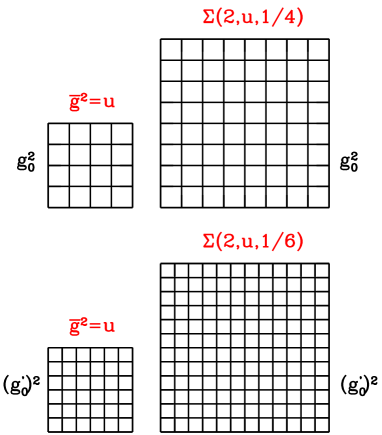
Figure 1: Illustration of the computation of the step scaling function, $\Sigma(u,a/L)$, at a fixed value of the coupling $u=\bar{g}^{2}(L)$ and for 2 lattice resolutions $L/a=4,6$ (cf. text).

Hence if we start with a lattice size $L/a=4$, measure $u=\bar{g}^{2}(L)$ in a numerical simulation and then measure $\bar{g}^{2}(2L)$ by doubling the lattice size to $2L/a$ (at the same value of the bare coupling $g_{0}$), we obtain a first approximant, $\Sigma(u,1/4)$, for $\sigma(u)$, where the second argument is the resolution $a/L$. We now want to keep $L$ constant in physical units but choose an $L/a=6$ lattice. This means we have to tune the bare coupling to another value $g_{0}^{\prime}$ such that the previous $u$-value is matched (which implicitly fixes $L$). Then, at the same $g_{0}^{\prime}$ one doubles the lattice size and measures the SF coupling to obtain $\Sigma(u,1/6)$. Continuing the procedure one may take the limit,

$$\sigma(u)=\lim_{a/L\rightarrow 0}\Sigma(u,a/L)\,,$$ (22)

at the given value of $u$. Repeating the same procedure for a range of $u$-values one obtains the function $\sigma(u)$ for this range with a certain error, due to both statistics and systematic effects from the continuum extrapolation. Once $\sigma(u)$ is available for a range of values $u\in[u_{\text{min}},u_{0}]$ one may iteratively step up the energy scale:

$$u_{0}=\bar{g}^{2}(L_{0}),\quad u_{n}=\sigma(u_{n+1})=\bar{g}^{2}(L_{n})=\bar{g}^{2}(2^{-n}L_{0}),\quad n=0,1,...$$ (23)

In particular, by construction the scale ratios are $L_{0}/L_{n}=2^{n}$, where $n$ is the number of steps.

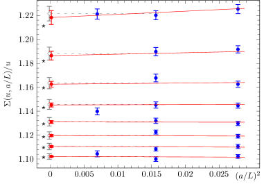
Figure 2: Continuum extrapolation of the step scaling function. Some data points have been slightly shifted in order to keep constant $u$, which is not required for the global fit. The leftmost points are the continuum values, whereas the stars are obtained from perturbative scale evolution using the 3-loop $\beta$-function.

7 Continuum extrapolation of $\Sigma(u,a/L)$

The lattice step-scaling function $\Sigma(u,a/L)$ is expected to be a smooth function of $u$. Lattice effects are, up to slowly varying logarithmic terms, polynomial in $a/L$. Moreover, terms linear in $a/L$ are removed in the bulk by the use of the non-perturbatively O($a$) improved action Yamada:2004ja , and highly suppressed at the time boundaries by using perturbative estimates of the counterterm coefficients. As a safeguard against any residual O($a$) effects we treat a variation of the 2 counterterm coefficients as a systematic effect and propagate it to the data. Rather than extrapolating the step-scaling function separately for individual values of $u$ it is more practical to use a global fit ansatz. A typical example is

$$\Sigma(u,a/L)=u+s_{0}u^{2}+s_{1}u^{3}+{c_{1}}u^{4}+{c_{2}}u^{5}+{\rho_{1}}u^{4}\dfrac{a^{2}}{L^{2}}+{\rho_{2}}u^{5}\dfrac{a^{2}}{L^{2}}$$ (24)

with $s_{0}$, $s_{1}$ fixed to perturbative values,

$$s_{0}=2b_{0}\ln 2,\quad s_{1}=s_{0}^{2}+2b_{1}\ln 2\,.$$ (25)

Our data for $\Sigma(u,a/L)$ has $L/a=4,6,8$ and, for a couple of $u$-values we have $L/a=12$. As a safeguard we omit the coarsest lattices with $L/a=4$ and fit the 19 data points to the above fit ansatz with 4 free parameters, $c_{1},c_{2},\rho_{1},\rho_{2}$. Fig. 2 shows the data together with the fit function. The $\chi^{2}/\text{d.o.f.}\approx 1$ for this and a variety of different fit ansätze indicates that we have a good control over the continuum limit. The continuum SSF is then represented by $\sigma(u)=u+s_{0}u^{2}+s_{1}u^{3}+c_{1}u^{4}+c_{2}u^{5}$, in the fit range $[1.02,2.02]$ and with numerical values for $c_{1},c_{2}$, together with their errors and correlation. The continuum step-scaling function can be compared with earlier results in Aoki:2009tf . where an attempt is made to reach larger couplings so as to match hadronic scales. In the high energy regime we have significantly improved on the precision both in terms of statistical and systematic errors, for instance through a very precise tuning to zero quark mass PatrickTomaszinpreparation .

8 Results

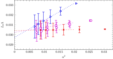
Figure 3: The extraction of the $\Lambda$-parameter using perturbation theory at various values of $\alpha_{s}$, plotted vs. $\alpha_{s}^{2}$. The data points are, from top to bottom, for $\nu=-0.5,0,0.3$ and, from right to left, for $n=0,1,\ldots,5$ steps by a factor 2 in scale. Nice agreement is observed around $\alpha_{s}\approx 0.1$.

The step scaling functions have been analysed for a number of $\nu$-values of O(1). Using eq. (18) for $L_{0}\Lambda$ we use non-perturbative running between $L_{0}$ and $L_{n}=2^{-n}L_{0}$, with $n=0,1,\ldots,5$. In physical units $1/L_{0}$ is about 4 GeV, so that we cover a range from 4 to 128 GeV. For a given $n$ we then integrate the integral in the exponent using the $\beta$-function to 3-loop order. In fig. 3 the results obtained at various $n$ and the 3 values $\nu=0,0.3,-0.5$ are plotted vs. $\alpha_{s}^{2}$, which is the order of the neglected terms. Up to such terms all the data points should agree within errors. The expected asymptotic behaviour is indeed observed. We see that for $\nu=0.3$ the slope in $\alpha_{s}^{2}$ is essentially zero, whereas it is rather large at $\nu=-0.5$. From fig. 3 and a variety of further fits not shown here we conclude that all results agree around $\alpha=0.1$ at the 3 percent level or better,

$$L_{0}\Lambda=0.0303(8)\quad\Leftrightarrow\quad L_{0}\Lambda_{\overline{\rm MS}}^{N_{\rm f}=3}=0.0791(21)\,.$$ (26)

While for $\nu=0.3$ this result could be inferred from larger values of $\alpha_{s}$, this is clearly not the case for $\nu=-0.5$. To further assess the accuracy of perturbation theory it is instructive to directly look at the second observable

$$\bar{v}(L)=\omega(u)|_{u=\bar{g}^{2}(L)}\,,$$ (27)

which allows us to study the couplings for all $\nu$-values (10) We have extrapolated the non-perturbative data to the continuum limit using similar global fits as for the step-scaling functions. However, here these fits are more constrained as there is no doubling of the lattice size involved and lattice sizes thus range from $L/a=6$ to $L/a=24$. Two resulting fit functions in the continuum limit of the form

$$\omega(u)|_{\text{fit 1}} = v_{1}+v_{2}u+d_{1}u^{2}+d_{2}u^{3}+d_{3}u^{4}\,,$$ (28)

$$\omega(u)|_{\text{fit 2}} = v_{1}+d_{1}u+d_{2}u^{2}+d_{3}u^{3}+d_{4}u^{4}\,,$$ (29)

with 3 and 4 fit parameters $d_{k}$, $k=1,\ldots$, respectively, are shown with their error bands in fig. 4. Both fits agree perfectly well in the whole range of the available non-perturbative data. The continuum result at $\bar{g}^{2}(L_{0})=2.012$,

$$\bar{v}(L_{0})=\omega(2.012)=0.1199(10),$$ (30)

is obtained from these fits and defines the starting values for the step-scaling procedure for $\nu\neq 0$ [cf. eq. (17)].

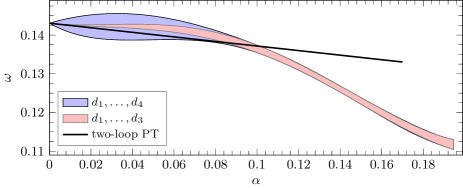
Figure 4: The observable, $\omega(u)=\bar{v}(L)$, plotted vs. $\alpha_{s}$, together with the fits eqs. (28,29) and the two-loop result (cf. text).

Fig. 4 also shows the known 2-loop result

$$\omega(u)=\left.\bar{v}\right|_{\bar{g}^{2}(1/L)=u,m=0}=v_{1}+v_{2}u+{\rm O}(u^{2})\,,$$ (31)

where the coefficients $v_{1},\,v_{2}$ can be found in DellaMorte:2004bc ). The non-perturbative data clearly breaks away from two-loop perturbation theory at larger couplings. To quantify this deviation we choose the value $\alpha_{s}=0.19$ and measure an effective 3-loop coefficient as follows

$$(\omega(\bar{g}^{2})-v_{1}-v_{2}\bar{g}^{2})/v_{1}=-3.7(2)\,\alpha_{s}^{2}\,.$$ (32)

Indeed this effective coefficient seems too large for perturbation theory to be trustworthy at this value of the coupling. We come to the conclusion that $\alpha\approx 0.1$ needs to be reached non-perturbatively for perturbation theory to become as accurate as we have required here.

9 Conclusions

We have pointed out that lattice observables can be defined at high energies if one gives up the requirement that volumes should be large enough to fit hadronic states. By defining observables in a finite volume it is possible to obtain non-perturbative precision data over a wide range of scales. Moreover, the heavy quark thresholds for charm and bottom can be “switched off" on the lattice, thereby removing an important source of systematic errors. The main drawback is that perturbation theory must match this situation and take the finite volume into account. This implies some technical difficulties which depend on all the details of the chosen set-up. With the SF scheme chosen here there exists a 2-loop calculation matching the SF couplings to the $\overline{\rm MS}$-scheme and thus the 3-loop $\beta$-function is known for a whole 1-parameter family of SF couplings. This provides excellent opportunities to test the accuracy of perturbation theory. As it turns out, a precision of 3 percent for the $\Lambda$-parameter can be quoted with confidence if perturbation theory is restricted to couplings around $\alpha_{s}\approx 0.1$ or smaller. However, at $\alpha_{s}\approx 0.2$ and to this level of accuracy there is much less confidence in perturbation theory and some luck is required when choosing a scheme.

Our result for the $\Lambda$-parameter, eq. (26), is an essential step in the ALPHA collaboration’s project to determine the $\Lambda$-parameter in 3-flavour QCD in units of a hadronic scale such as the kaon and pion decay constants, $F_{K,\pi}$. These are determined in large volumes Bruno:2016plf on gauge configurations produced through the CLS effort Bruno:2014jqa . Preliminary results have been presented by M. Dalla Brida at this conference and by R. Sommer in Bruno:2016gvs . An estimate of $\alpha_{s}(m_{Z})$ is given there, assuming that the standard perturbative treatment of the charm and bottom quark thresholds is reliable. While we have focussed here on the $\Lambda$-parameter and running couplings, an analogous study can be made for the running quark masses and first results have been presented by P. Fritzsch at this conference Campos:2016vxh .

Acknowledgments

This work was done as part of the ALPHA collaboration research programme. I would like to thank the members of the ALPHA collaboration and particularly my co-authors of ref. Brida:2016flw for the enjoyable collaboration on this project and for comments on the manuscript. Computer resources by the computer centres at HLRN (bep00040) and NIC at DESY, Zeuthen, as well as financial support by SFI under grant 11/RFP/PHY3218 are gratefully acknowledged.

References

- (1) M. Dalla Brida, P. Fritzsch, T. Korzec, A. Ramos, S. Sint, R. Sommer (ALPHA), Phys. Rev. Lett. 117, 182001 (2016), 1604.06193
- (2) M. Lüscher, Commun. Math. Phys. 104, 177 (1986)
- (3) S. Aoki et al., Eur. Phys. J. C74, 2890 (2014), 1310.8555
- (4) K. Jansen, C. Liu, M. Lüscher, H. Simma, S. Sint, R. Sommer, P. Weisz, U. Wolff, Phys. Lett. B372, 275 (1996), hep-lat/9512009
- (5) A. Pich, A. RodrÃguez-Sánchez, Phys. Rev. D94, 034027 (2016), 1605.06830
- (6) D. Boito, M. Golterman, K. Maltman, S. Peris (2016), 1611.03457
- (7) S. Weinberg, Phys. Rev. D8, 3497 (1973)
- (8) K. Symanzik, Nucl. Phys. B190, 1 (1981)
- (9) M. Lüscher, R. Narayanan, P. Weisz, U. Wolff, Nucl. Phys. B384, 168 (1992), hep-lat/9207009
- (10) S. Sint, Nucl. Phys. B421, 135 (1994), hep-lat/9312079
- (11) M. Lüscher, R. Sommer, P. Weisz, U. Wolff, Nucl. Phys. B413, 481 (1994), hep-lat/9309005
- (12) S. Sint, P. Vilaseca, PoS LATTICE2012, 031 (2012), 1211.0411
- (13) S. Sint, R. Sommer, Nucl. Phys. B465, 71 (1996), hep-lat/9508012
- (14) A. Bode, P. Weisz, U. Wolff (ALPHA), Nucl. Phys. B576, 517 (2000), [Erratum: Nucl. Phys.B608,481(2001)], hep-lat/9911018
- (15) M. Lüscher, P. Weisz, Phys. Lett. B349, 165 (1995), hep-lat/9502001
- (16) C. Christou, H. Panagopoulos, A. Feo, E. Vicari, Phys. Lett. B426, 121 (1998)
- (17) C. Christou, A. Feo, H. Panagopoulos, E. Vicari, Nucl. Phys. B525, 387 (1998), [Erratum: Nucl. Phys.B608,479(2001)], hep-lat/9801007
- (18) T. van Ritbergen, J.A.M. Vermaseren, S.A. Larin, Phys. Lett. B400, 379 (1997), hep-ph/9701390
- (19) M. Czakon, Nucl.Phys. B710, 485 (2005), hep-ph/0411261
- (20) M. Dalla Brida, P. Fritzsch, T. Korzec, A. Ramos, S. Sint, R. Sommer, in preparation
- (21) K.A. Olive et al. (Particle Data Group), Chin. Phys. C38, 090001 (2014)
- (22) M. Lüscher, P. Weisz, U. Wolff, Nucl. Phys. B359, 221 (1991)
- (23) N. Yamada et al. (JLQCD, CP-PACS), Phys.Rev. D71, 054505 (2005), hep-lat/0406028
- (24) S. Aoki et al. (PACS-CS), JHEP 0910, 053 (2009), 0906.3906
- (25) P. Fritzsch, T. Korzec, in preparation
- (26) M. Della Morte, R. Frezzotti, J. Heitger, J. Rolf, R. Sommer, U. Wolff (ALPHA), Nucl. Phys. B713, 378 (2005), hep-lat/0411025
- (27) M. Bruno, T. Korzec, S. Schaefer (2016), 1608.08900
- (28) M. Bruno et al., JHEP 02, 043 (2015), 1411.3982
- (29) M. Bruno, M. Dalla Brida, P. Fritzsch, T. Korzec, A. Ramos, S. Schaefer, H. Simma, S. Sint, R. Sommer, The determination of by the ALPHA collaboration, in 6th Workshop on Theory, Phenomenology and Experiments in Flavour Physics: Interplay of Flavour Physics with electroweak symmetry breaking (Capri 2016) Anacapri, Capri, Italy, June 11, 2016 (2016), 1611.05750, http://inspirehep.net/record/1498572/files/arXiv:1611.05750.pdf
- (30) I. Campos, P. Fritzsch, C. Pena, D. Preti, A. Ramos, T. Vladikas (2016), 1611.06102