RCSED – A Value-Added Reference Catalog of Spectral Energy Distributions of 800,299 Galaxies in 11 Ultraviolet, Optical, and Near-Infrared Bands: Morphologies, Colors, Ionized Gas and Stellar Populations Properties

Abstract

We present RCSED, the value-added Reference Catalog of Spectral Energy Distributions of galaxies, which contains homogenized spectrophotometric data for 800,299 low and intermediate redshift galaxies ($0.007<z<0.6$) selected from the Sloan Digital Sky Survey spectroscopic sample. Accessible from the Virtual Observatory (VO) and complemented with detailed information on galaxy properties obtained with the state-of-the-art data analysis, RCSED enables direct studies of galaxy formation and evolution during the last 5 Gyr. We provide tabulated color transformations for galaxies of different morphologies and luminosities and analytic expressions for the red sequence shape in different colors. RCSED comprises integrated $k$-corrected photometry in up-to 11 ultraviolet, optical, and near-infrared bands published by the GALEX, SDSS, and UKIDSS wide-field imaging surveys; results of the stellar population fitting of SDSS spectra including best-fitting templates, velocity dispersions, parameterized star formation histories, and stellar metallicities computed for instantaneous starburst and exponentially declining star formation models; parametric and non-parametric emission line fluxes and profiles; and gas phase metallicities. We link RCSED to the Galaxy Zoo morphological classification and galaxy bulge+disk decomposition results by Simard et al. We construct the color–magnitude, Faber–Jackson, mass–metallicity relations, compare them with the literature and discuss systematic errors of galaxy properties presented in our catalog. RCSED is accessible from the project web-site and via VO simple spectrum access and table access services using VO compliant applications. We describe several SQL query examples against the database. Finally, we briefly discuss existing and future scientific applications of RCSED and prospectives for the catalog extension to higher redshifts and different wavelengths.

1. Introduction and Motivation

During the last decade we witnessed a breakthrough in wide field imaging surveys across the electromagnetic spectrum. The new era started with the Sloan Digital Sky Survey (SDSS) that used a 2.5-m telescope and covered over 11,600 sq. deg. of the sky in 5 optical photometric bands ($ugriz$) down to the 22nd AB magnitude in its latest 7th legacy data release (Abazajian et al., 2009). It had a spectroscopic follow-up survey that targeted over 1 million galaxies and quasars and half a million stars down to the magnitude limit of $r=17.77$ AB mag. Even though by the end of 2015, the data from SDSS and its successors, SDSS-II, and SDSS-III were used in about 20,000 research papers, the SDSS potential for scientific exploration remains far from exhaustion.

In the late 2000s, deep wide field surveys went beyond the optical spectral domain. The Galaxy Evolution Explorer (GALEX) satellite (Martin et al., 2005) provided nearly all-sky photometric coverage in two ultraviolet bands centered at 154 and 228 nm down to the limiting magnitudes $AB=20.5$ mag. The SDSS footprint area was observed by GALEX with 15 times longer exposure that yielded a much deeper limit of $AB=23.5$ mag. The relatively small telescope provided the spatial resolution of a couple of arcsec comparable to the typical image quality level at ground-based facilities.

At the same time, a major effort was undertaken by the international team at the 4-m United Kingdom Infrared Telescope UKIRT to survey a substantial area of the sky largely overlapping with the SDSS footprint in 4 near-infrared (NIR) bands ($YJHK$). The Large Area Survey of the UKIRT Deep Sky Survey (UKIDSS LAS, Lawrence et al., 2007) provides a sub-arcsecond resolution and the flux limit comparable to that of SDSS in the optical domain. It reaches $AB\sim 21.2$ mag, 3–4 mag deeper than the first all-sky NIR survey 2MASS (Skrutskie et al., 2006).

Numerous projects studied the entire SDSS spectroscopic sample of galaxies by analyzing both absorption (see e.g. Kauffmann et al., 2003; Gallazzi et al., 2006) and emission lines (Brinchmann et al., 2004; Tremonti et al., 2004; Oh et al., 2011, 2015) in SDSS spectra (MPA-JHU and OSSY catalogs). However, they did not make use of any additional information beyond that available in the SDSS database.

The first successful attempt of providing an added value to SDSS data was done a decade ago in the “New York University Value-Added Galaxy Catalog” (NYU-VAGC) project (Blanton et al., 2005). It was aimed at statistical studies of galaxy properties and the large scale structure of the Universe and included a compilation of information derived from photometry and spectroscopy in one of the earlier SDSS data releases (that represents about 20% of its final imaging footprint). It also comprised positional cross matches with 2MASS, far-infrared IRAS point source catalog (Saunders et al., 2000), the Faint Images of the Radio sky 20 cm survey FIRST (Becker et al., 1995), and additional data on galaxies from the 3rd Reference Catalogue of Bright Galaxies (de Vaucouleurs et al., 1991) and the Two-Degree Field Galaxy Redshift Survey (Colless et al., 2001). Now, a decade after the NYU-VAGC has been published, there is a sharp need to assemble a next generation of a value-added galaxy catalog based on modern survey data that were not available back then.

Here we present a new generation and a different flavor of a value-added catalog of galaxies based on a combination of data from SDSS, GALEX, and UKIDSS surveys that also includes comprehensive analysis of absorption and emission lines in galaxy spectra. Our main motivation is to use the synergy provided by the joint panchromatic dataset for extragalactic astrophysics: the optical domain is traditionally the best studied and there exist well calibrated stellar population models; the UV fluxes are sensitive to even small fractions of recently formed stars and therefore contain valuable information on star formation histories; the near-IR band is substantially less sensitive to the internal dust reddening and stellar population ages, and therefore can provide good stellar mass estimates. Our mission is to build a reference multi-wavelength spectrophotometric dataset and complement it with additional detailed information on galaxy properties so that it will allow astronomers to study galaxy formation and evolution at redshifts $z=0.0\textup{--}0.6$ in a transparent way with as little extra manipulations as possible.

We aim to provide: (i) the first homogeneous set of low redshift galaxy FUV-to-NIR spectral energy distributions (SEDs) corrected to rest frame for hundreds of thousands of objects; (ii) the first photometric dataset containing rest frame aperture SEDs with corresponding spectra and their stellar population analysis: velocity dispersions, parameterized star formation histories; (iii) consistent analysis of absorption and emission lines in SDSS galaxy spectra including parametric and non-parametric emission line fitting performed using state-of-the-art stellar population models, which cover a wider range of ages and metallicities and, therefore, help to minimize the template mismatch; (iv) easy and fully Virtual Observatory compliant data access mechanisms for our dataset and several third-party catalogs that include morphological and structural information for galaxies in our sample.

We started this project in 2009 by developing a new approach to convert galaxy SEDs to the rest frame by calculating analytic approximations of $k$-corrections in optical and NIR bands (Chilingarian et al., 2010). Then we extended our algorithm to GALEX FUV and NUV bands and discovered a universal 3-dimensional relation of NUV and optical galaxy colors and luminosities (Chilingarian & Zolotukhin, 2012). Then, we fitted SDSS spectra using state-of-the-art stellar population models, derived velocity dispersions and stellar ages and metallicities, and provided our measurements to the project that calibrated the fundamental plane of galaxies (Djorgovski & Davis, 1987) in SDSS by vigorous statistical analysis (Saulder et al., 2013). Our dataset also helped to find and characterize massive compact early-type galaxies at intermediate redshifts (Damjanov et al., 2013, 2014). Finally, we used a complex set of selection criteria and discovered a large sample of previously considered extremely rare compact elliptical galaxies (Chilingarian & Zolotukhin, 2015).

The paper is organized as follows: in Section 2 we describe the construction of the catalog that includes cross-matching of the three surveys, adding third-party catalogs, absorption and emission line analysis of SDSS spectra; in Section 3 we discuss the photometric properties of the sample and derive mean colors of galaxies of different morphological types across the spectrum; in Section 4 we explore the information derived from our spectral analysis; Section 5 contains the description of the catalog access interfaces; Section 6 provides the summary of our project; and Appendices include some technical details on the catalog construction, detailed description of tables included in the database, and discussion of systematic uncertainties of emission line measurements.

2. Construction of the catalog

2.1. The input sample and data sources used.

We compiled the photometric catalog by re-processing several publicly available datasets. Our core object list is the SDSS Data Release 7 (Abazajian et al., 2009) spectral sample of non-active galaxies (marked as “GAL_EM” or “GALAXY” specclass in the SDSS database) in the redshift range $0.007\leq z<0.6$. We provide the exact query that we used to select this sample in the SDSS CasJobs Data System in Appendix B. The query executed in the DR7 CasJobs context returned 800,299 records. We deliberately excluded quasars and Seyfert-1 galaxies (specclass=“QSO”) because neither the $k$-correction technique, nor stellar population analysis algorithm supported that object type. We used the output table as an input list for positional cross-matches against GALEX Data Release 6 (Martin et al., 2005) and UKIDSS Data Release 10 (Lawrence et al., 2007).

For the UKIDSS cross-match we queried the UKIDSS Large Area Survey catalog using the best match criterion within a 3 arcsec radius. In order to perform this query, we employed the WFCAM Science Archive for the programmatic access to the International Virtual Observatory Alliance (IVOA) ConeSearch service with a multiple cone search (“multi-cone”) capability. The query returned 280,870 UKIDSS objects matching the galaxies from our input sample. We used the stilts software package (Taylor, 2006) in order to access the UKIDSS data and merge the tables.

Then we uploaded the input SDSS galaxy list to the GALEX CasJobs web interface and searched best matches within 3 arcsec similarly to the UKIDSS cross-match. The query returned 485,996 GALEX objects.

As a result of this selection procedure we compiled an input catalog of 800,299 spectroscopically confirmed SDSS galaxies, out of which 90,717 have 11 band photometry (two GALEX FUV and NUV, 5 SDSS $ugriz$ bands, 4 UKIDSS $YJHK$ bands), 163,709 have all UKIDSS bands and at least one UV band, 582,534 have at least one additional photometric band to SDSS bands. In Fig. 1 we present the footprint of our catalog on the all-sky aitoff projection marking the regions covered by all three wide field imaging surveys using different colors. The statistics of galaxies measured in different photometric bands is given in Table 1.

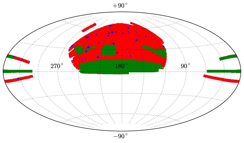
Figure 1.— A full sky aitoff projection in equatorial coordinates demonstrating the footprint of our catalog. Green areas denote the availability of all three input photometric datasets, SDSS, UKIDSS, and GALEX; red areas are for SDSS and GALEX; and blue areas are for SDSS only. Note that we include all objects from the input datasets that have at least one flux measurement in them.

Table 1Number of objects in the combined sample with photometric measurements available from three input photometric catalogs.

Photometric bands	Number of galaxies
SDSS $ugriz$	799783
GALEX $FUV$ + $ugriz$	286570
GALEX $NUV$ + $ugriz$	469419
$FUV$ + $NUV$ + $ugriz$	270152
$ugriz$ + UKIDSS $Y$	270603
$ugriz$ + UKIDSS $J$	265316
$ugriz$ + UKIDSS $H$	272028
$ugriz$ + UKIDSS $K$	273050
$ugriz+YJHK$	250608
$NUV+ugriz+YJHK$	157531
all 11 bands	90717

Then we linked the following published datasets to our catalog in order to contribute the spectrophotometric information with some of the most widely used galaxy properties: (i) the results of the two-dimensional light profile decomposition of SDSS galaxies by Simard et al. (2011) that include structural properties of all objects in our catalog; (ii) the morphological classification table from the citizen science “Galaxy Zoo” project (Lintott et al., 2008, 2011) that provides a human eye classification of well spatially resolved SDSS galaxies made by citizen scientists. 661,319 objects in our sample have 10 or more morphological classifications in the Galaxy Zoo catalog ($nvote\geq 10$).

2.2. The photometric catalog

2.2.1 Petrosian and aperture magnitudes

All three photometric surveys used in our study provide extended source photometry along with aperture measurements made in several different aperture sizes (GALEX and UKIDSS).

For the SED photometric analysis and construction of scaling relations involving galaxy luminosity, we need total magnitudes. For this purpose we adopt Petrosian (1976) magnitudes available in SDSS and UKIDSS as measurements which do not significantly depend on galaxy light profile shapes conversely to SDSS modelmags (see discussion in Chilingarian & Zolotukhin, 2012). The GALEX catalog provides “total” magnitudes that are close to Petrosian magnitudes for exponential surface brightness profiles (i.e. disc galaxies) and up-to 0.2 mag brighter for elliptical galaxies (Yasuda et al., 2001). However, given the average photometric uncertainty in the GALEX $NUV$ fluxes of red galaxies of $0.3$ mag, we can neglect this difference.

On the other hand, our parent sample of galaxies was derived from the SDSS spectroscopic sample, and all SDSS DR7 spectra were obtained in circular 3-arcsec wide apertures. Therefore, we need 3-arcsec aperture magnitudes in order to make quantitative comparison of spectroscopic and photometric data. Hence, we computed aperture magnitudes for all GALEX and UKIDSS sources with available aperture measurements by interpolating the flux to a 3-arcsec aperture, and used SDSS fibermags for the optical SED part. To be noticed, that the spatial resolution of the GALEX survey in the $NUV$ band is about 5 arcsec, therefore 3-arcsec aperture magnitudes will be slightly underestimated for small objects. For compact (point-like) sources a 3-arcsec aperture $NUV$ magnitude can be underestimated by as much as 0.3 mag, however, such objects are very rare in the SDSS DR7 galaxy sample. Damjanov et al. (2013); Zahid et al. (2015, 2016) found a couple of thousands compact sources in SDSS and SDSS-iii BOSS, only a few hundreds of which were in SDSS DR7. We estimated a number of compact galaxies in our sample by selecting the sources where the average difference of aperture and Petrosian magnitudes in $ugriz$ bands was $<0.3$ mag: this query returned 831 objects or $<0.1$% of the sample.

We corrected the obtained sets of Petrosian and 3-arcsec aperture magnitudes for the Galactic foreground extinction by using the $E(B-V)$ values computed from the Schlegel et al. (1998) extinction maps. Then, we computed $k$-corrections for both sets of photometric points using the analytic approximations presented in Chilingarian et al. (2010) and updated for $GALEX$ bands in Chilingarian & Zolotukhin (2012).

In Fig. 2 we provide an example of a fully corrected SED for a late type spiral galaxy ($z=0.035$) that has flux measurements in all 11 bands. We show both total and fiber magnitudes and overplot an SDSS spectrum with the wavelength axis converted into the rest frame and fluxes converted into $AB$ magnitudes. One can see a remarkable agreement between the corrected photometric points and the observed spectral flux density, typical for our catalog.

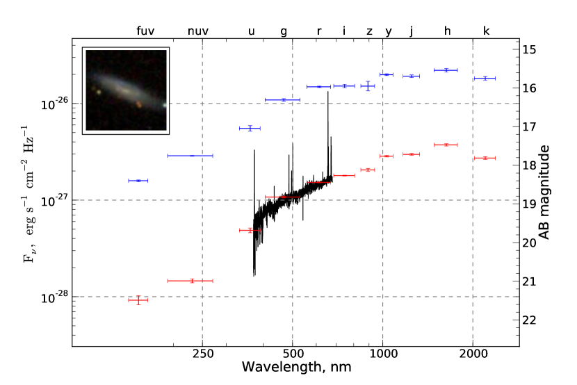
Figure 2.— Example of fully corrected SED in 11 bands for a late type spiral galaxy at redshift 0.035. Blue and red symbols represent total (Petrosian) and 3-arcsec fiber magnitudes correspondingly. The rest framed SDSS spectrum is overplotted and demonstrates a typical excellent agreement with the corrected fiber magnitudes for that galaxy. The inset shows an 36$\times$36 arcsec optical SDSS false color image.

2.2.2 Correcting the SDSS–UKIDSS photometric offset

An important problem of the UKIDSS photometric catalog of extended sources is the observed spread of colors including optical SDSS and NIR UKIDSS photometric measurements (e.g. $g-J$ for red sequence galaxies). We detected this inconsistency in Chilingarian et al. (2010) and applied an empirical correction to UKIDSS magnitudes based on the assumption of continuous SEDs of galaxies. We computed $z-Y$ colors by interpolating over all other available colors approximating the SED with a low order polynomial function. This approach, however, required the availability of the $Y$ band photometry in the UKIDSS catalog. We have analyzed the SDSS–UKIDSS Petrosian magnitude offset amplitude for different galaxies and concluded, that it originates from the surface brightness limitation imposed by relatively short integration time in UKIDSS and by high and variable sky background level in the NIR. Therefore, Petrosian radii and magnitudes become underestimated, and comparison of original UKIDSS extended source magnitudes with SDSS and GALEX integrated photometry becomes impossible, because any color including data from UKIDSS and another data source depends on the galaxy surface brightness and size.

Here we propose a general and simple empirical solution. We exploit the UKIDSS Galactic Cluster Survey photometric catalog that includes the $Z$ band photometry, convert it into SDSS $z$ with the available color transformation (Hewett et al., 2006) for both Petrosian and 3-arcsec aperture magnitudes, and compare it to actual SDSS $z$ band measurements from the SDSS DR7 catalog for exactly the same objects. It turns out, that (i) the Petrosian magnitude difference $z_{\mathrm{SDSS,Petro}}-z_{\mathrm{UKIDSS,Petro}}$ correlates with the galaxy mean surface brightness; (ii) the fiber magnitude difference $z_{\mathrm{SDSS,fib}}-z_{\mathrm{UKIDSS,3^{\prime\prime}}}$ is close to zero within 0.02 mag; (iii) differences between Petrosian and fiber magnitudes in all UKIDSS photometric bands ($ZYJHK$) are almost identical that indicates virtually flat NIR color profiles in most galaxies. This suggests that the correction for UKIDSS Petrosian magnitudes should be calculated as: $\Delta(mag_{\mathrm{UKIDSS,Petro}})=(z_{\mathrm{SDSS,fib}}-z_{\mathrm{SDSS,Petro}})-(Y_{\mathrm{UKIDSS,3^{\prime\prime}}}-Y_{\mathrm{UKIDSS,Petro}})$. This transformation adjusts the UKIDSS integrated photometry in a way that the differences between the 3 arcsec and Petrosian magnitudes of a galaxy in $z$ and $Y$ bands become equal. For objects, where $Y$ magnitudes are not available in the UKIDSS survey, we use the next available photometric band ($J$, $H$, or $K$).

In this fashion, we obtained fully corrected FUV-to-NIR spectral energy distributions converted into rest-frame magnitudes for a large sample of galaxies in 3-arcsec apertures and integrated over entire galaxies.

2.3. The spectral catalog: absorption lines

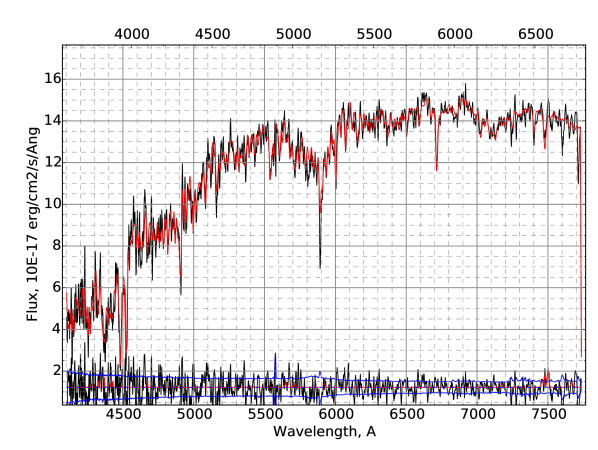
Figure 3.— Example of the nbursts full spectrum fitting for an SDSS spectrum of an early type galaxy. An observed galaxy spectrum is shown in black, the best fitting template is in red, residuals are in blue. Regions of emission lines excluded from the fitting are shown red in the residuals. The observed and rest-frame wavelength are shown in the bottom and top of the plot respectively.

We fitted all SDSS spectra using the nbursts full spectrum fitting technique (Chilingarian et al., 2007a, b) and determined their radial velocities $v$, stellar velocity dispersions $\sigma$, and parameterized star formation histories represented by an instantaneous star burst (simple stellar populations, SSP) or an exponentially declining star formation history (exp-SFH) assuming that it started shortly after the Big Bang. We chose these two families of stellar population models because: (i) SSP models are widely used in extragalactic studies by different authors and we wanted our data to be directly comparable to other sources; (ii) exponentially declining SFHs were demonstrated to be a better representation of broadband SEDs of non-active galaxies (Chilingarian & Zolotukhin, 2012) than SSPs. We should, however, notice, that exp-SFH models cannot adequately describe young stellar populations with mean ages $t<1.5$ Gyr (see discussion below).

The fitting procedure first convolves a grid of stellar population models with the wavelength dependent spectral line spread function available for every SDSS spectrum in the original data files, then runs a non-linear Levenberg-Markquardt minimization by first choosing a model spectrum from the grid by two-dimensional interpolation in the age–metallicity ($t$–[Fe/H]) space, then convolving it with a Gaussian-Hermite representation of the line-of-sight velocity distribution (LOSVD) of stars in a galaxy described by $v,\sigma,h3,h4$, and finally multiplying it by a low order Legendre polynomial continuum (its parameters are determined linearly in a separate loop) in order to absorb flux calibration imperfections and possible internal extinction in a galaxy. Hence, the procedure returns values of $v,\sigma,h3,h4,t,$[Fe/H], and coefficients of the multiplicative polynomial continuum. Here we use a pure Gaussian LOSVD shape with $h3=h4=0$.

The nbursts algorithm is similar to the penalized pixel fitting approach by Cappellari & Emsellem (2004). It, however, has some important differences. (i) We use a linear fit of the low order multiplicative polynomial continuum because its parameters are decoupled from galaxy kinematics and stellar populations. (ii) Instead of using a fixed grid of template spectra and interpreting stellar populations using their relative weights in a linear combination, we interpolate in a grid of models inside the minimization loop in order to obtain the best-fitting stellar population parameters of each starburst (or an exponentially declining model). As a result, for the simplest case of a single component SSP model, we obtain the best-fitting SSP-equivalent age and metallicity. These values are usually close to the luminosity weighted ones, however, in cases of complex SFHs approximated by an SSP there might be biases similar to those affecting Lick indices (Serra & Trager, 2007). Chilingarian et al. (2007b, 2008) demonstrated that SSP equivalent ages and metallicity remain unbiased for galaxies with super-solar $\alpha$-element abundances ([Mg/Fe]$>$0 dex) and when Balmer line regions are masked in order to fit emission lines.

We excluded the spectral regions affected by bright atmosphere lines (Oi, NaD, OH, etc.) and by the $A$ and $B$ telluric absorption bands from the fitting procedure. We also re-ran the fitting code excluding $8\textup{--}14$ Å-wide regions around locations of bright emission lines for objects, where the reduced $\chi^{2}$ value of the fit exceeded the threshold $\chi^{2}/DOF=$0.8, that was selected empirically from a sample of galaxies without and with emission lines of different intensity levels.

We used three grids of stellar population models all computed with the pegase.hr evolutionary synthesis code (Le Borgne et al., 2004):

1. SSP models based on the high resolution (R=10000) ELODIE.3.1 empirical stellar library (Prugniel & Soubiran, 2004; Prugniel et al., 2007) covering the wavelength range $3900<\lambda<6800$ Å, the metallicity range $-2.5<$[Fe/H]$<0.5$ dex, and ages $20<t<20000$ Myr.

2. Models with exponentially declining SFH at a constant metallicity computed for the same metallicity and wavelength ranges as those for SSP models, covering the range of exponential decay timescales $10<\tau<20600$ Myr (the latter one effectively being a constant star formation rate model) and starting epochs of star formation between $4.3$ Gyr and $13.8$ Gyr of the age of the Universe corresponding to the redshift range $0<z<1.5$. We used the exponential decay timescale $\tau$ in the same fashion as the SSP age in the minimization procedure. For every galaxy, we first computed a grid of $\tau-$[Fe/H] models with the star formation epoch corresponding to its redshift assuming that a galaxy was formed at very high redshift, e.g. for $z=0.2$ with the light travel time of 2.45 Gyr, we computed a grid of models for star formation that started 11.27 Gyr ago assuming the standard WMAP9 cosmology (Hinshaw et al., 2013).

3. Intermediate resolution SSP models ($R=2300$) based on the MILES empirical stellar library (Sánchez-Blázquez et al., 2006) covering the wavelength range $3600<\lambda<7400$ Å, the metallicity range $-2.5<$[Fe/H]$<0.7$ dex, and ages $20<t<20000$ Myr.

We stress that the best-fitting stellar population ages $t>14000$ Myr (SSP) and exponential timescales $\tau<1000$ Myr (exp-SFH) should be considered as upper and lower limits for the corresponding parameters.

In the public version of our catalog we provide two sets of stellar population parameters for every galaxy: (1) SSP ages and metallicities obtained from the spectrum fitting in the wavelength range in a galaxy rest-frame $4500<\lambda<6795$ Å using the MILES-pegase.hr models with the 5-th degree of the multiplicative polynomial continuum; (2) pegase.hr based exponentially declining SFR models in the wavelength range $3915<\lambda<6795$ Å with the 19-th degree continuum. The 19-th degree corresponds to the emipirically determined optimal degree of the multiplicative polynomial continuum for SDSS spectra when the $\chi^{2}$ value reaches a “plateau” as explained in Chilingarian et al. (2008). We performed the SSP fitting with the MILES-pegase.hr models in the truncated wavelength range with a very low order polynomial continuum in order to minimize the artifacts originating from imperfections in the SSP model grid (see Section 4.2). In the publicly available Simple Spectrum Access Service we provide the results of the MILES-pegase.hr based SSP fitting in the wavelength range $3600<\lambda<6790$ Å in order to enable the emission line analysis from the fitting residuals for all lines including the [Oii] 3727 Å doublet.

2.4. The spectral catalog: emission lines

Our full spectral fitting procedure precisely matches the stellar continuum of each galaxy by the best-fitting stellar population model (see example in Fig. 3). Although the regions of all Balmer absorption lines are age sensitive, they contain at most 20% of the age sensitive information from the entire optical spectral range (Chilingarian, 2009). Chilingarian et al. (2007b) have demonstrated that masking the H$\beta$ and H$\gamma$ regions biases neither age nor metallicity determinations by the nbursts procedure. Hence, we do not expect to introduce significant template mismatch by masking the regions of emission lines when fitting SDSS spectra. Having subtracted the best-fitting model we obtain clean emission line spectra unaffected by stellar absorptions that is especially important for the Balmer lines. The precision of our stellar continuum fitting allows us to recover faint emission lines at a few per cent level of the continuum intensity, whereas very often such lines are not detected in the SDSS spectral pipeline results. In Table 2 we provide the statistics of the emission line detection and strength in our sample.

In order to measure fluxes and equivalent widths (EW) of emission lines we applied two different approaches, namely Gaussian and non-parametric fitting of emission lines profiles.

In some galaxies, emission lines profiles cannot be described by a Gaussian. This often becomes a case in galaxies with peculiar gas kinematics, e.g. multi-component bulk gas motions and outflows can produce complex asymmetric lines. Also, this is crucially important for active galactic nuclei (AGN) with broad components in Balmer lines. Approximation of such emission lines by a Gaussian profile results in biased estimates of flux and kinematic parameters. We address this problem by employing a non-parametric fitting approach which allows us to recover arbitrary line profiles and measure their fluxes with higher precision. At the same time, this method requires several lines with sufficiently high signal-to-noise ratio to be present in a spectrum, and may produce biased results when dealing with noisy data. We, therefore, perform a “classical” Gaussian profile fitting too in order to allow for cross-comparison and validation of our line fitting results.

Both non-parametric and Gaussian fitting techniques take into account the SDSS line-spread function computed individually for each spectrum by the standard SDSS pipeline and provided in FITS (Flexible Image Transport System) tables in the RCSED distribution.

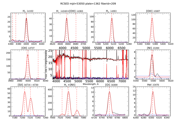
Figure 4.— Example of the nbursts full spectrum fitting for an SDSS spectrum of a late type galaxy together with the emission line fitting. Central panel is similar to Fig. 3, panels on the sides demonstrate recovered profiles after the continuum subtraction of individual emission lines (black) and the best-fitting models (red). Blue lines show emission line flux uncertainties. Vertical red dashed lines represent the galaxy redshift in the SDSS database.

2.4.1 Gaussian fitting

This approach consists of simultaneously fitting the entire set of emission lines (see the line list in Table 2) with Gaussians pre-convolved with the SDSS line-spread function. We allow two different sets of redshifts and intrinsic widths for recombination and forbidden lines. We estimate the kinematic parameters with the non-linear least-square minimization that is implemented by the MPFIT package (Markwardt, 2009). The emission line fluxes are computed linearly for each minimization iteration. When solving the linear problem, we constrain the line fluxes to be non-negative. For this purpose we use the BVLS (bounded-variables least-squares) algorithm (Lawson & Hanson, 1995) and its implementation by M. Cappellari.

Table 2Emission line detection statistics (the parametric Gaussian fit) at different signal-to-noise ratio (SNR). The “Covered” column reflects the number of objects with a corresponding line in the wavelength coverage. The “Wavelength” column provides air wavelengths. The “Prefix” column gives the prefix of column names for the corresponding spectral line in the emission line FITS tables from the RCSED distribution.

Line	Wavelength	Prefix	Covered	$SNR>1$		$SNR>3$		$SNR>5$		$SNR>10$
	Å		N	N	fraction	N	fraction	N	fraction	N	fraction
[O ii]	3726.03	f3727_oii	780665	543374	69.6%	354307	45.4%	225669	28.9%	92161	11.81%
[O ii]	3728.82	f3730_oii	782417	562707	71.9%	387264	49.5%	257713	32.9%	110287	14.10%
H$\kappa$	3750.15	f3751_h_kappa	791720	233850	29.5%	26219	3.3%	5584	0.7%	535	0.07%
H$\iota$	3770.63	f3772_h_iota	796081	180306	22.6%	18912	2.4%	4524	0.6%	595	0.07%
H$\theta$	3797.90	f3799_h_theta	798386	229961	28.8%	31590	4.0%	8466	1.1%	1345	0.17%
H$\eta$	3835.38	f3836_h_eta	798565	255213	32.0%	52680	6.6%	16876	2.1%	2976	0.37%
[Ne iii]	3868.76	f3870_neiii	798635	246202	30.8%	45733	5.7%	19500	2.4%	7579	0.95%
He i	3887.90	f3889_hei	798674	182764	22.9%	37166	4.7%	10644	1.3%	1328	0.17%
H$\zeta$	3889.07	f3890_h_zeta	798675	223107	27.9%	63940	8.0%	26166	3.3%	6072	0.76%
H$\epsilon$	3970.08	f3971_h_epsilon	798835	360759	45.2%	156226	19.6%	78430	9.8%	21312	2.67%
[S ii]	4068.60	f4070_sii	799003	202235	25.3%	14766	1.8%	2352	0.3%	149	0.02%
[S ii]	4076.35	f4078_sii	799010	149342	18.7%	4755	0.6%	517	0.1%	55	0.01%
H$\delta$	4101.73	f4103_h_delta	799043	342858	42.9%	172913	21.6%	96748	12.1%	32463	4.06%
H$\gamma$	4340.46	f4342_h_gamma	799276	419668	52.5%	275775	34.5%	192540	24.1%	87637	10.96%
[O iii]	4363.21	f4364_oiii	799293	118667	14.8%	8001	1.0%	2569	0.3%	787	0.10%
He ii	4685.76	f4687_heii	799381	109369	13.7%	6779	0.8%	2204	0.3%	614	0.08%
[Ar iv]	4711.37	f4713_ariv	799381	79310	9.9%	3477	0.4%	530	0.1%	110	0.01%
[Ar iv]	4740.17	f4742_ariv	799380	118077	14.8%	7031	0.9%	1108	0.1%	85	0.01%
H$\beta$	4861.36	f4863_h_beta	799375	514321	64.3%	381556	47.7%	317350	39.7%	214953	26.89%
[O iii]	4958.91	f4960_oiii	799372	449021	56.2%	164285	20.6%	92442	11.6%	47287	5.92%
[O iii]	5006.84	f5008_oiii	799371	638852	79.9%	404135	50.6%	244845	30.6%	119215	14.91%
[N i]	5197.90	f5199_ni	799360	144430	18.1%	9742	1.2%	1345	0.2%	178	0.02%
[N i]	5200.25	f5202_ni	799360	184255	23.1%	16318	2.0%	2676	0.3%	226	0.03%
[N ii]	5754.59	f5756_nii	799131	196670	24.6%	12800	1.6%	2763	0.3%	966	0.12%
He i	5875.62	f5877_hei	798546	260312	32.6%	81904	10.3%	38829	4.9%	12209	1.53%
[O i]	6300.30	f6302_oi	784763	439640	56.0%	177144	22.6%	77850	9.9%	16856	2.15%
[O i]	6363.78	f6366_oi	780219	285886	36.6%	40626	5.2%	9143	1.2%	1395	0.18%
[N ii]	6548.05	f6550_nii	764832	596254	78.0%	422810	55.3%	289961	37.9%	133553	17.46%
H$\alpha$	6562.79	f6565_h_alpha	763451	614029	80.4%	531966	69.7%	479842	62.9%	395722	51.83%
[N ii]	6583.45	f6585_nii	761376	641883	84.3%	553212	72.7%	479386	63.0%	334901	43.99%
He i	6678.15	f6679_hei	750612	178330	23.8%	21069	2.8%	6321	0.8%	1408	0.19%
[S ii]	6716.43	f6718_sii	745687	571758	76.7%	423064	56.7%	320126	42.9%	186973	25.07%
[S ii]	6730.81	f6733_sii	743742	554071	74.5%	374143	50.3%	263155	35.4%	135572	18.23%

2.4.2 Non-parametric emission line fitting

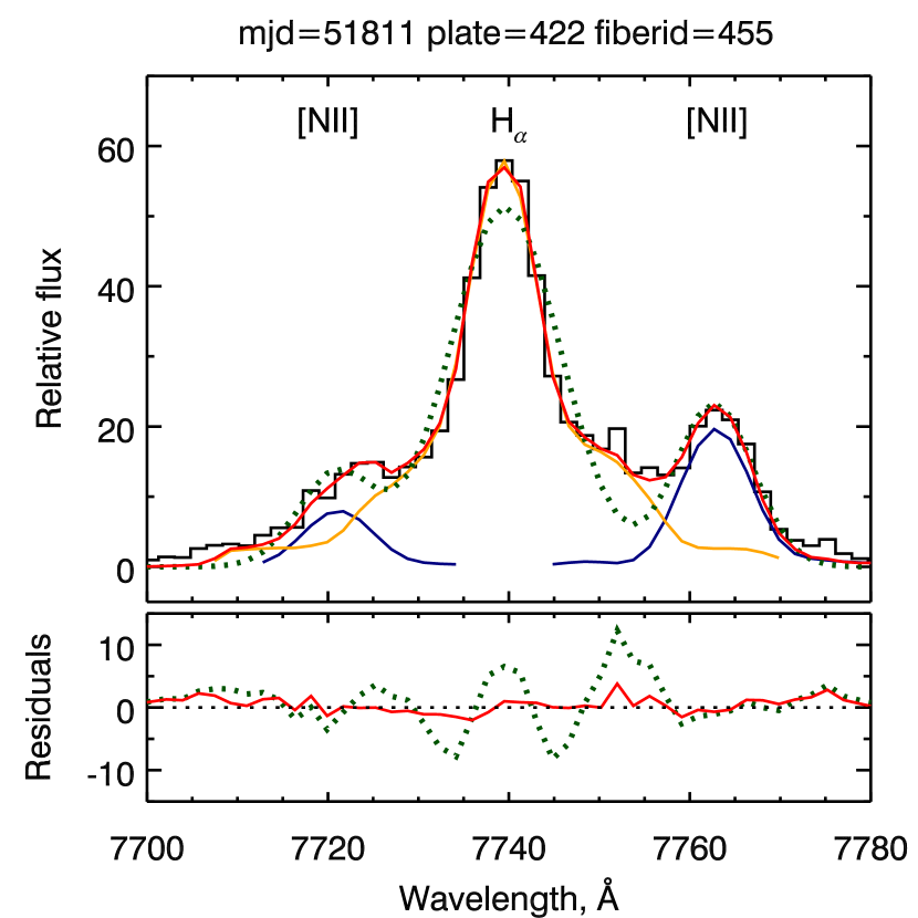
Figure 5.— An example of the complex emission line profile of a Seyfert galaxy, and results of its fitting with two different techniques. Black stepped line in the upper panel shows the observed spectrum of H$\alpha$ and Nii lines in relative flux units, green dotted line is a Gaussian fit result, red solid line is a non-parametric fitting result. Individual H$\alpha$ and Nii profiles recovered by the non-parametric fitting are shown in orange and blue respectively. Lower panel shows fitting residuals. In the case of complex asymmetric emission lines profiles non-parametric fitting method is clearly preferred over Gaussian one.

Our non-parametric emission line fitting method includes two main steps which we repeat several times until the convergence is achieved. First, we derive discretely sampled emission line profiles, i.e. line-of-sight velocity distributions (LOSVDs) of ionized gas. During the second step, we estimate emission lines fluxes. Because allowed and forbidden transitions often originate from different regions of a galaxy having very different physical properties (i.e. density, temperature, mechanism of excitation), however, all emission lines of each type (allowed and forbidden) have similar shapes, our procedure recovers two different non-parametric profiles, one for each type.

The LOSVD derivation is organized as follows. We note that convolution of any logarithmically rebinned observed spectrum $S_{obs}$ of $m$ elements with LOSVD $\mathcal{L}$ having $n$ elements can be expressed as a linear matrix equation $A\ast\mathcal{L}=S_{obs}$, where $A$ is a $m\times n$ matrix of template spectra having lengths of $m$ pixels each. Every template spectrum from the $i$-th row in the matrix $A$ is shifted by the velocity which represents the $i$-th position within the LOSVD vector. Here a template spectrum is a synthetic spectrum made of a set of flux normalized Gaussians with LSF widths representing emission lines detected in the observed spectrum. Such approach allows us to take into account the SDSS instrumental resolution instead of a set of Dirac $\delta$-functions. The continuum level of a template spectrum is set to zero.

Thus, we end up with a linear inverse problem whose solution $\mathcal{L}$ can be derived by a least square technique. The emission line profiles obviously cannot be negative and, therefore, we use the BVLS algorithm mentioned above.

Once the LOSVD has been derived, we compute emission line fluxes by solving a similar linear problem to that described in Section 2.4.1. This finishes the first iteration.

At the same time, the LOSVD derivation step requires the knowledge of emission line fluxes in order to construct better template spectra. During the first iteration when they are unknown, we set all fluxes to unity and the all template spectra hence are made of equally normalized Gaussians. Typically, 3 iterations of this procedure is enough to reach the convergence.

A linear inversion is an ill-conditioned problem and is sensitive to noise in the data. In order to improve the profile reconstruction quality, we exploit a regularization technique, which minimizes the squared third derivative of the recovered line profile. This approach, however, causes artefacts in sharp narrow line profiles. Therefore, we apply the regularization only in the wings of emission lines where flux levels are generally low and, consequently, noise is higher. The regularization technique yields the dramatic improvement of recovered Balmer line profiles for faint AGNs. In the catalog we provide measurements of non-parametric emission lines with and without regularization.

The comparison between the parametric (Gaussian) and non-parametric fitting results for a complex emission line profile in a Seyfert galaxy is presented at Fig. 5. A Gaussian approximation for such lines is often inadequate and causes serious biases in the kinematics that can reach few hundred km s^-1.

We ran Monte-Carlo simulations for a random sample of 2,000 objects with emission lines of different intensity levels in order to estimate realistic flux uncertainties obtained with the non-parametric fitting technique. They turned out to be consistent with statistical uncertainties of Gaussian emission line fluxes for most objects and up-to a factor of 2 lower for AGNs with broad line components. The RCSED database will be updated with Monte-Carlo based uncertainties as we compute them: this procedure is very computationally intensive and will take a couple of months to complete.

2.4.3 Gas phase metallicities

We used our emission line flux measurements in order to estimate the gas phase metallicities for galaxies where emissions originate from the star formation induced excitation. We exploited two different techniques to measure the metallicity, (i) a new calibration by Dopita et al. (2016) and (ii) the IZI Bayesian technique (Blanc et al., 2015) using a grid of models ($\kappa=\infty$) with $\kappa$-distributed electron energies (Dopita et al., 2013). We selected star formation dominated and “transition type” galaxies using the standard BPT (Baldwin et al., 1981) diagram that exploits hydrogen, nitrogen, and oxygen emission lines with the criteria defined in Kauffmann et al. (2003).

The Dopita et al. (2016) calibration uses only the H$\alpha$, [Nii], and [Sii] emission lines, all located in a very narrow spectral interval and is, therefore, virtually insensitive to the internal extinction within an observed galaxy. This calibration is presented in a form of a simple formula which makes it very easy to use. However, a disadvantage of this approach in application to our dataset is that at redshifts $z>0.1$ the emission lines used for the metallicity determination shift to the spectral region dominated by telluric absorption and airglow emission lines (mostly, OH) which can seriously affect the quality of the emission line flux estimates. Another natural limitation of this approach originates from the SDSS spectral wavelength range ($\lambda<9200$ Å) that corresponds to the upper redshift limit $z=0.36$ when the forbidden sulfur line [Sii] 6730 Å shifts out of the wavelength range. Besides, the calibration critically depends on the [N/O] relation and is therefore sensitive to possible galaxy to galaxy [N/H] abundance variations. In the catalog we included the metallicity estimates obtained using the Dopita et al. (2016) calibration for Gaussian emission line analysis (rcsed_gasmet table). We computed the uncertainties of the gas phase metallicities by propagating the statistical flux errors through the calculations according to the formula in Dopita et al. (2016).

The IZI technique (Blanc et al., 2015) takes advantage of all available emission line measurements and, hence, is more robust and can in principle be used for the entire sample of SDSS galaxies. The algorithm is implemented in an idl software package distributed by the authors along with 17 grids of photoionization models. However, this technique relies on the external dust attenuation correction which must be applied to emission lines fluxes prior to fitting. It also requires (similar to the Dopita et al. (2016) approach) a pre-selection of star forming galaxies. We estimated the internal dust attenuation using the typical value of the Balmer decrement H$\alpha$/H$\beta=2.83$ (Groves et al., 2012) and corrected all emission line fluxes accordingly. In galaxies where the observed H$\alpha$/H$\beta$ ratio fell below that value, we assumed the extinction to be zero. Finally, the fluxes were supplied to the IZI software package with the Dopita et al. (2013) model grid and the resulting [O/H] and ionizing parameter values for Gaussian emission line fluxes were included in the gas phase metallicity table rcsed_gasmet of the catalog.

3. Photometric properties of the sample

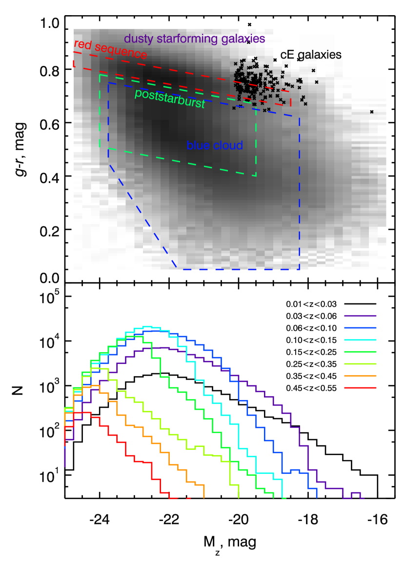
Figure 6.— (Top) Optical color–magnitude diagram for extinction- and $k$-corrected Petrosian magnitudes of all galaxies in our sample. (Bottom) Redshift distributions of galaxies in corresponding bins on absolute magnitude.

3.1. Completeness at different redshifts

Because our catalog uses the SDSS DR7 spectroscopic galaxy sample as its master list, and the legacy SDSS spectroscopic survey was magnitude limited with the $r=17.77$ mag limit in a 3 arcsec aperture, we sample different parts of the galaxy luminosity function with the redshift dependent completeness. Also, there is an important fiber collision effect, that is when two fibers in the SDSS multi-object spectrograph cannot be put too close to each other: because of this, there is a systematic undersampling of dense clusters and groups of galaxies.

In Fig. 6 (top panel) we present a two-dimensional distribution of our galaxies in the $(M_{z},g-r)$ color–magnitude space. We identify the regions traditionally referred to as “the red sequence” and “the blue cloud” as well as the locus of typical post-starburst (E+A) galaxies. The density in the plot corresponds to the object number density in our catalog at a given position of the parameter space. We also show by small crosses the tidally stripped systems, compact elliptical galaxies, from the sample of Chilingarian & Zolotukhin (2015) which reside systematically above the red sequence. One can see the bimodality of the galaxy distribution by color for intermediate luminosity and dwarf galaxies ($M_{z}>-20.5$ mag) while the transition is rather smooth for more luminous systems.

Even though dwarf galaxies are more numerous in the Universe than giants because of the raising low end of the galaxy luminosity function (Schechter, 1976; Blanton et al., 2003), we see the apparent decrease of the histogram density at fainter magnitudes. In the bottom panel of Fig. 6 we demonstrate the breakdown by redshift for the luminosity distribution of galaxies contributing to the histogram in the top panel. The high luminosity end decline is due to the intrinsic shape of the luminosity function, while the low luminosity tail drops because of the SDSS completeness and target selection biased against very extended (and therefore nearby) galaxies. We clearly see how the magnitude limit constraint of SDSS causes the drop in the number of galaxies further and further up the luminosity function as we move to higher redshifts. Fig. 6 confirms that we start probing the dwarf galaxy regime ($M_{z}>-19.8$ mag) at $z<0.06$, however the selection effects have to be seriously considered for any type of a statistical study.

3.2. Red sequence in different bands

For practical reasons such as selection of candidate early-type members in galaxy clusters using photometric data, it is important to know the shape of the red sequence in different photometric bands. Here we provide the best fitting second degree polynomial approximations of the red sequence shape for a set of galaxy colors spanning optical and NIR bands.

First we created a sample of red sequence galaxies by the following criteria: (1) We selected all objects at redshifts $z<0.27$; (2) we applied a color cut on $NUV-r$ colors by selecting all objects on $(M_{r},NUV-r)$ plane that resided above the straight line passing through $p_{0}=(-16.0,3.5)$ mag and $p_{1}=(-24.0,5.0)$ mag; (3) we applied a color cut on $g-r$ colors by selecting all objects on $(M_{r},g-r)$ plane that resided above the straight line passing through $q_{0}=(-16.0,0.5)$ mag and $q_{1}=(-24.0,0.75)$ mag and also satisfying the criterion $(g-r)<0.95$ mag.

Then, in order to account for two orders of magnitude variations of galaxy density along the red sequence, for every combination of colors and magnitudes (e.g. $g-r$, $M_{r}$): (1) We selected measurements having statistical uncertainties $<0.1$ mag in both bands; (2) binned the distribution on luminosity using 0.5 mag wide bins and computed median color values and outlier resistant standard deviations in every bin; (3) fitted a second degree polynomial into median values only in those bins that contained more than 15 objects. For convenience and because mean absolute $AB$ magnitudes of galaxies in our sample stay mostly within the range $-25<M<-15$ mag in all optical red ($riz$) and NIR filters, we added 20.0 mag to all absolute magnitudes prior to fitting.

$$(u-r) =+2.51-0.065\cdot M_{20r}-0.005\cdot M_{20r}^{2};\,\sigma=0.16$$

$$(u-i) =+2.90-0.069\cdot M_{20i}-0.007\cdot M_{20i}^{2};\,\sigma=0.17$$

$$(u-z) =+3.15-0.050\cdot M_{20z}-0.014\cdot M_{20z}^{2};\,\sigma=0.19$$

$$(g-r) =+0.75-0.026\cdot M_{20r}-0.001\cdot M_{20r}^{2};\,\sigma=0.045$$

$$(g-i) =+1.12-0.038\cdot M_{20i}-0.003\cdot M_{20i}^{2};\,\sigma=0.074$$

$$(g-z) =+1.39-0.044\cdot M_{20z}-0.009\cdot M_{20z}^{2};\,\sigma=0.10$$

$$(g-Y) =+1.91-0.067\cdot M_{20Y}-0.018\cdot M_{20Y}^{2};\,\sigma=0.14$$

$$(g-J) =+2.01-0.073\cdot M_{20J}-0.016\cdot M_{20J}^{2};\,\sigma=0.18$$

$$(g-H) =+2.30-0.094\cdot M_{20H}-0.015\cdot M_{20H}^{2};\,\sigma=0.19$$

$$(g-K) =+2.00-0.108\cdot M_{20K}-0.018\cdot M_{20K}^{2};\,\sigma=0.22$$

$$M_{20\mathrm{col}}=M_{\mathrm{col}}+20.0\mathrm{mag}$$ (1)

Eqs. 1 provide the best-fitting polynomials for the red sequence shape in 10 photometric bands. We consider the mean standard deviation value from all bins used in the fitting procedure as the “red sequence width” ($\sigma$ in Eqs. 1) and stress that the actual fitting residuals for median values are usually an order of magnitude smaller.

We notice that in the most widely used parameter spaces, $(M_{r},g-r)$, $(M_{r},u-r)$, $(M_{i},g-i)$, and $(M_{z},g-z)$, the red sequence does not show any substantial curvature which is indicated by negligible 2nd order polynomial terms. This suggests that there is no “red sequence saturation” at the bright end.

3.3. Color transformations for galaxies of different morphologies and luminosities

Table 3Median rest-frame colors of galaxies of different morphological types and luminosities in $AB$ magnitudes. For every color (left column) there are three groups corresponding to giant (1st group), intermediate luminosity (2nd group), and dwarf (3rd group) galaxies of 6 values for 6 Hubble types. Standard deviation values for each median color are presented in the adjacent table rows.

	$-24.0\leq M_{r}<-22.0$ mag						$-22.0\leq M_{r}<-19.0$ mag						$-19.0\leq M_{r}<-16.0$ mag
	Sdm	Sc	Sb	Sa	S0	E	Sdm	Sc	Sb	Sa	S0	E	Sdm	Sc	Sb	Sa	S0	E
$FUV$-$r$	1.72	2.76	3.46	4.33	5.58	6.86	1.60	2.48	3.22	4.15	5.22	6.72	1.44	2.18	2.87	3.81	4.91	6.78
stdev	0.33	0.33	0.40	0.50	0.78	0.67	0.31	0.32	0.39	0.48	0.71	0.78	0.26	0.31	0.36	0.46	0.75	0.91
$NUV$-$r$	1.20	2.20	2.89	3.73	4.84	5.64	1.17	2.02	2.69	3.57	4.57	5.44	1.15	1.80	2.41	3.29	4.18	4.98
stdev	0.26	0.20	0.27	0.29	0.30	0.25	0.22	0.24	0.27	0.28	0.29	0.27	0.18	0.23	0.24	0.25	0.26	0.25
$u$-$r$	0.99	1.48	1.80	2.14	2.44	2.56	0.95	1.34	1.68	2.05	2.32	2.44	0.88	1.19	1.44	1.76	2.02	2.14
stdev	0.15	0.19	0.21	0.21	0.23	0.19	0.19	0.20	0.20	0.21	0.21	0.17	0.26	0.20	0.19	0.22	0.24	0.21
$g$-$r$	0.26	0.49	0.60	0.70	0.78	0.80	0.24	0.40	0.53	0.65	0.73	0.76	0.22	0.34	0.45	0.57	0.66	0.69
stdev	0.15	0.06	0.05	0.05	0.05	0.03	0.09	0.07	0.06	0.05	0.05	0.04	0.10	0.06	0.06	0.06	0.06	0.04
$g$-$i$	0.42	0.75	0.92	1.06	1.15	1.17	0.33	0.58	0.81	1.00	1.10	1.12	0.26	0.45	0.64	0.85	0.98	1.02
stdev	0.27	0.11	0.09	0.07	0.07	0.05	0.16	0.12	0.11	0.08	0.08	0.06	0.16	0.11	0.10	0.11	0.10	0.07
$g$-$z$	0.66	0.97	1.16	1.32	1.42	1.44	0.41	0.72	1.02	1.25	1.37	1.39	0.33	0.55	0.79	1.05	1.18	1.24
stdev	0.32	0.18	0.14	0.11	0.10	0.07	0.21	0.18	0.16	0.12	0.11	0.09	0.21	0.18	0.16	0.16	0.15	0.10
$g$-$Y$	1.27	1.50	1.70	1.87	1.97	1.98	0.78	1.12	1.50	1.79	1.91	1.92	0.59	0.82	1.12	1.46	1.58	1.68
stdev	0.45	0.19	0.17	0.13	0.12	0.09	0.31	0.27	0.22	0.16	0.14	0.12	0.33	0.28	0.26	0.26	0.23	0.15
$g$-$J$	1.37	1.56	1.77	1.96	2.05	2.07	0.83	1.15	1.58	1.90	2.01	2.03	0.53	0.77	1.11	1.51	1.66	1.75
stdev	0.46	0.23	0.21	0.17	0.16	0.13	0.38	0.35	0.27	0.19	0.18	0.15	0.49	0.46	0.39	0.36	0.32	0.22
$g$-$H$	1.63	1.87	2.10	2.30	2.39	2.40	1.05	1.42	1.89	2.22	2.33	2.33	0.77	1.02	1.37	1.80	1.89	1.99
stdev	0.54	0.24	0.21	0.18	0.17	0.14	0.39	0.35	0.27	0.21	0.20	0.16	0.47	0.38	0.34	0.36	0.32	0.20
$g$-$K$	1.54	1.61	1.83	2.03	2.11	2.11	0.80	1.12	1.60	1.95	2.04	2.03	0.34	0.62	1.00	1.44	1.55	1.63
stdev	0.52	0.25	0.23	0.19	0.18	0.15	0.45	0.40	0.30	0.24	0.23	0.18	0.56	0.49	0.42	0.44	0.36	0.24

Chilingarian & Zolotukhin (2012) demonstrated that the Hubble morphological classification derived by a human eye (Fukugita et al., 2007) correlates very well with the total $NUV-r$ color of a galaxy. With a computed dispersion of $0.8t$, where $t$ is the Hubble type, it corresponds to the subjective precision of such a classification. Here we use this relation in order to derive median values of galaxy colors across the Hubble sequence for three galaxy luminosity classes defined on a basis of their $r$-band luminosities.

We dissect the $(M_{r},NUV-r)$ color–magnitude plane into 18 quadrangular regions by assuming that the morphological type for giant galaxies ($M_{r}=-24$ mag) can be estimated by linearly varying the $(NUV-r)$ color from $+0.5$ to $+6.5$ mag with a step of 1 mag corresponding to one Hubble type from Sd to E. At the same time, we assume that in the dwarf regime $(M_{r}=-16$ mag) the step reduces to 0.75 mag per Hubble type that corresponds to the observed reduction of the $(NUV-r)$ color range. We choose 3 luminosity bins, $-24.0\leq M_{r}<-22.0$ mag, $-22.0\leq M_{r}<-19.0$ mag, and $-19.0\leq M_{r}<-16.0$ mag, which represent giant, intermediate luminosity, and dwarf galaxies. Then, in every region we compute the median value of a desired color, and the standard deviation of the distribution.

We present our results in Table 3. They expand and update the widely used color transformations from Fukugita et al. (1995) by using a very rich dataset properly corrected for systematic effects and using modern prescriptions for $k$-corrections. We extend their results at $z=0$ (see table 3 in Fukugita et al., 1995) to near-UV and NIR colors and also towards intermediate and low luminosity galaxies. The direct comparison of our values with those of Fukugita et al. (1995) reveals a good agreement of optical colors except (a) S0 galaxies which are systematically redder in our case and stay really close to the ellipticals; (b) the $u-g$ color of ellipticals that is some 0.25 mag bluer in our case. We assign the latter systematics to our improved $k$-correction prescriptions for the $u$ band photometry and generally higher quality of the $u$ band SDSS photometric data compared to the dataset used in Fukugita et al. (1995). On the other hand, we attribute redder colors of lenticular galaxies in our data to the specificities of the synthetic color estimation technique used in Fukugita et al. (1995) that underestimated colors of 2 of 4 their lenticular galaxies by 0.1–0.15 mag (see their table 1).

4. Spectroscopic properties of the sample

4.1. Stellar kinematics of galaxies

In comparison to original SDSS measurements of stellar kinematics based on cross-correlation with a limited set of template spectra, our approach yields significantly smaller template mismatch between models and observed spectra for non-active galaxies. We, therefore, achieve on average 30% lower statistical uncertainties of radial velocity and velocity dispersion measurements. Moreover, there is a known degeneracy between stellar metallicity and velocity dispersion estimates when using pixel space fitting techniques (Chilingarian et al., 2007b), because an underestimated metallicity (i.e. using a metal poor template for a metal rich galaxy) can be compensated by a lower velocity dispersion that would smear that template spectrum to a lesser degree. Therefore, by using a grid of stellar population models ranging from low ([Fe/H]$=-2.0$ dex) to high ([Fe/H]$=+0.7$ dex) metallicities and covering the whole range of ages, we reduce the systematic errors of velocity dispersion measurements, especially in the most metal-rich regime including massive elliptical and lenticular galaxies. On the other hand, we accurately take into account the spectral line spread function of the SDSS spectrograph that allows us to measure velocity dispersions down to 50 km s^-1, thus going far into the dwarf galaxy regime (Chilingarian, 2009).

As it was already pointed out by Fabricant et al. (2013), stellar velocity dispersion measurements in the SDSS DR7 catalog are systematically underestimated for luminous elliptical galaxies compared to the values obtained by the full spectrum fitting, that is likely caused by the template mismatch and degeneracy with metallicity mentioned above. Here we observe a very similar trend: our SSP velocity dispersion measurements for massive ellipticals ($\sigma\mathrel{\hbox{\hbox to0.0pt{\hbox{\lower 4.0pt\hbox{$\sim$}}\hss}\hbox{$>$}}}250$ km s^-1) are up-to 30 km s^-1 higher than those reported in the SDSS DR7 catalog, and this difference goes down to 7–10 km s^-1 for low luminosity galaxies ($\sigma\sim 100$ km s^-1). In Fig. 7 (top panel) we present the comparison made for our entire sample for 361,421 galaxies with velocity dispersion uncertainties better than 7% of the value (i.e. $\Delta\sigma=$7 km s^-1 for $\sigma=100$ km s^-1). The velocity dispersions estimated from the fitting of exponentially declining SFH models computed with pegase.hr, are a little bit closer to the values in SDSS DR7, however, the general trend looks similar (Fig. 7, bottom panel).

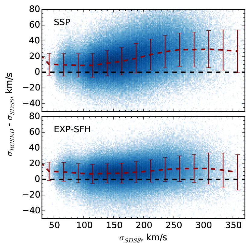
Figure 7.— Comparison of RCSED stellar velocity dispersion measurements with those published by the SDSS DR7. Top and bottom panel correspond to the two sets of stellar population models, SSP and exponentially declining SFHs correspondingly.

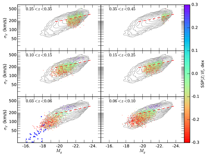
Figure 8.— Faber–Jackson relation for 52,506 morphologically classified elliptical galaxies in our sample (Galaxy Zoo classification). In order to remove outliers, a 10$\%$ cut has been applied on the relative errors on g magnitude and on the velocity dispersion and a good adjustment has been required $\chi^{2}<0.8$. The contours correspond to the whole sample (smoothed with a 3$\times$3-pixels window). Each panel displays a redshift range corresponding to Figure 6. The color coding corresponds to the SSP metallicity $[Z/H]$ displayed in Figure 10. The dashed red line corresponds to the maximum likelihood estimate of the slope $L_{g}\propto\sigma^{4.00}$ at $z=0$ computed by Bernardi et al. (2003). The blue points in the low redshift sub-sample (in the bottom left panel) correspond to the dwarf galaxies sample of Chilingarian et al. (2008).

In Fig. 8 we present the relation between galaxy luminosities and velocity dispersions or the Faber–Jackson (1976) relation constructed for 52,506 elliptical galaxies which were morphologically selected by the Galaxy Zoo (Lintott et al., 2011) citizen science project and had statistical uncertainties of their velocity dispersion measurements better than 10% of the value. We have corrected velocity dispersion measurements to their global values according to Cappellari et al. (2006) using half-light radii from Simard et al. (2011) included in our catalog. We used the criterion formulated in Saulder et al. (2013): in order to be included in our early type galaxy sample, an object has to be classified by at least 10 Galaxy Zoo users of whom at least 70% classify it as an elliptical galaxy. Six panels present measurements in six different redshift intervals shown as dots while the contours display the cumulative distribution at all redshifts. The lowest redshift panel contains the measurements for a sample of galaxies in the Abell 496 cluster ($z=0.033$) obtained from the analysis of intermediate resolution (R=6300) spectra collected with the FLAMES–Giraffe spectrograph at the 8-m Very Large Telescope of the European Southern Observatory (Chilingarian et al., 2008). This dataset comprises mostly dwarf early-type galaxies and it clearly forms an extension of the low–luminosity part of the relation formed by the SDSS galaxies which demonstrates that our velocity dispersion measurements at the low end do not suffer from systematic errors connected to the spectral line spread function uncertainties. The red dashed line represents the Faber–Jackson relation for giant elliptical galaxies $L_{g}\propto\sigma^{4.00}$ at $z=0$ presented in Bernardi et al. (2003). We see that the slope changes to $L_{g}\propto\sigma^{2.00}$ at fainter luminosities $M_{g}>-19.5$ mag similar to what was demonstrated for a sample of dwarf galaxies in the Coma galaxy cluster by Matković & Guzmán (2005).

Because of the correlation of a galaxy luminosity with a stellar velocity dispersion and the magnitude limited input galaxy sample, higher redshift galaxies contribute only to the bins at high stellar velocity dispersions. Our catalog probes dwarf galaxies ($\sigma<100$ km s^-1) at low redshifts ($0.007<z<0.06$) that includes hundreds of massive galaxy clusters and groups.

RCSED velocity dispersion measurements were used prior to publication by Saulder et al. (2013) for the calibration of the Fundamental Plane (Djorgovski & Davis, 1987). We refer to that work for an intensive discussion regarding the FP of elliptical galaxies observed by the SDSS.

4.2. Stellar populations from absorption line analysis

In our catalog we include stellar population parameters obtained by the fitting of galaxy spectra using two stellar population model grids computed with the pegase.hr evolutionary synthesis code: (i) SSP models based on the intermediate resolution MILES stellar library characterized by ages ($t$) and metallicities ([Fe/H]); and (ii) models with exponentially declining SFHs based on the high resolution ELODIE-3.1 stellar library characterized by exponential timescales ($\tau$) and metallicities ([Fe/H]). In Fig 9 we present distributions of galaxies in the two parameter spaces.

One can clearly see a spotty structure in the SSP best fitting results and the lack of such a structure for the exponentially decaying models. We also performed similar tests for original MILES stellar population models by Vazdekis et al. (2010) and models by Bruzual & Charlot (2003) for a sub-sample of SDSS DR7 spectra. We will provide a complete description and detailed discussion in the forthcoming paper (Katkov et al. in prep.), here we present a brief summary and conclusions of our study.

The observed spotty structure represents artifacts caused by the improper implementation of the interpolation algorithm in the stellar population code most likely on the stellar library interpolation step propagating into stellar population models and not by the nbursts population fitting procedure. The nbursts code uses a non-linear minimization technique that requires the second partial derivatives on all parameters to be continuous. Discontinuities will cause the solution to be either attracted to some region of the parameter space, or pushed away from it.

Our conclusion is supported by the following observations: (i) the morphology of the spotty structure remains very similar when using two different sets of SSP models computed with the same pegase.hr code but with different stellar libraries, MILES and ELODIE; (ii) switching to original MILES models (Vazdekis et al., 2010) where the interpolation procedure is much simpler than in pegase.hr (linear interpolation between 5 nearest neighbors) changes the structure completely and strengthens the artifacts; (iii) using exponentially decaying star formation models which are constructed of numerous weighted SSPs removes most of the pattern at $\tau\mathrel{\hbox{\hbox to0.0pt{\hbox{\lower 4.0pt\hbox{$\sim$}}\hss}\hbox{$>$}}}1.0$ Gyr but the structure still holds at $\tau<1.0$ Gyr where the number of co-added SSPs is small; (iv) smoothing a grid of pegase.hr MILES based SSP models using basic splines ($b$-splines) on age removes most of the pattern.

We also notice, that extending the working wavelength range to shorter wavelengths ($<4500$ Å) and increasing the multiplicative polynomial degree strengthens the pattern while leaving spot positions in the pattern virtually the same. Therefore, we chose a very low order 5-th degree polynomial continuum and restricted the wavelength range to $\lambda>4500$ Å for the SSP fitting that produced stellar population parameters presented in our catalog.

In the top panel of Fig. 10, we present the comparison of SSP ages and exponential timescales $\tau$. Despite the artifact structure in ages that extends into horizontal stripes on this plot, there is a 1-to-1 correspondence between $t$ and $\tau$ in a wide range of ages. Short timescales $\tau$ correspond to old stellar populations while $\tau=20$ Gyr is equivalent to $t\approx 1.8$ Gyr. The relation “saturates” for younger stellar populations because they cannot be represented by exponentially declining SFHs starting at high redshifts: either a later start or multiple star formation episodes are needed to describe them. Chilingarian & Zolotukhin (2012) demonstrated that exponentially declining SFHs much better represent observed broadband optical and UV colors than SSP models. In our current sample about 16% of galaxies ($\sim$131,500) have stellar populations too young too be described by exponentially declining SFHs.

The bottom panel of Fig. 10 displays the comparison of stellar metallicities for the two sets of models. The agreement is very good with a slight systematic difference between $-0.6<$[Fe/H]$<-0.2$ dex which we attribute to the degeneracy between the metallicity and velocity dispersion measurements for intermediate signal-to-noise ratios.

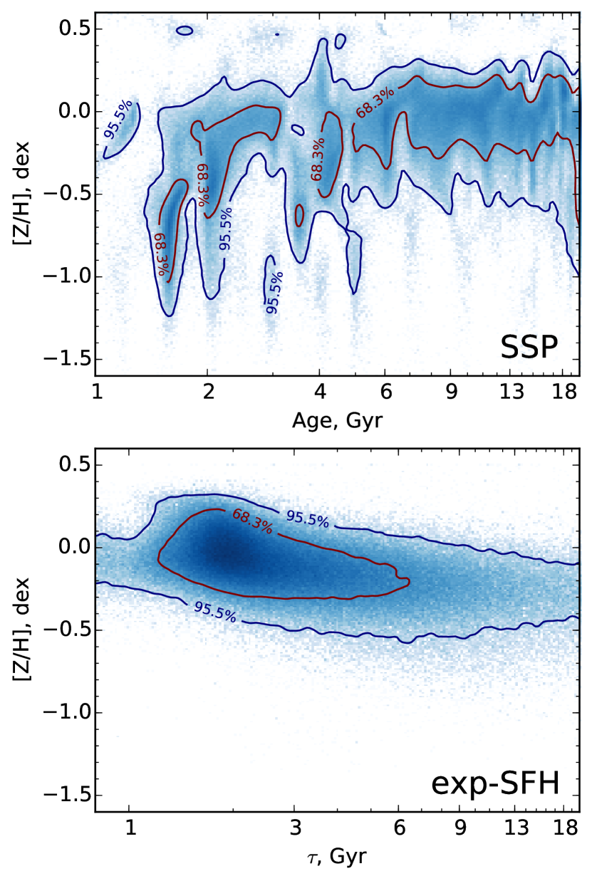
Figure 9.— Distributions of galaxies in the age–metallicity space from the fitting of SSP (top panel) and exponentially decaying SFH (bottom panel) models.

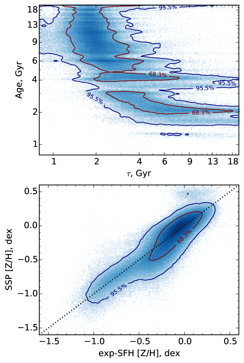
Figure 10.— Comparison of SSP ages to timescales $\tau$ for exponentially decaying models (top) and metallicity measurements (bottom).

We clearly see a substantial degeneracy between the metallicity and velocity dispersion estimates which was pointed out in Chilingarian et al. (2007b). In order to perform a clear test, free of any effects connected to the usage of different star formation histories, we fitted a subset of $\sim$420,000 spectra using pegase.hr SSP models in the wavelength range 3910–6790 Å and compared the metallicity and velocity dispersion measurements to those obtained from the fitting of MILES–pegase models against the same spectra. In Fig. 11 we present the relation between the differences of velocity dispersions and SSP metallicities obtained using the two sets of models at different signal-to-noise ratios. We can clearly see the degeneracy manifested by the elongated shape of the cloud that decreases with the increasing signal-to-noise ratio up-to the signal-to-noise of 30. Above 30 the improvement becomes insignificant. This result suggest that published velocity dispersion values obtained with the full spectral fitting of intermediate resolution spectra $R=1500-2500$ are subject to serious systematic errors reaching 15% of the measured value.

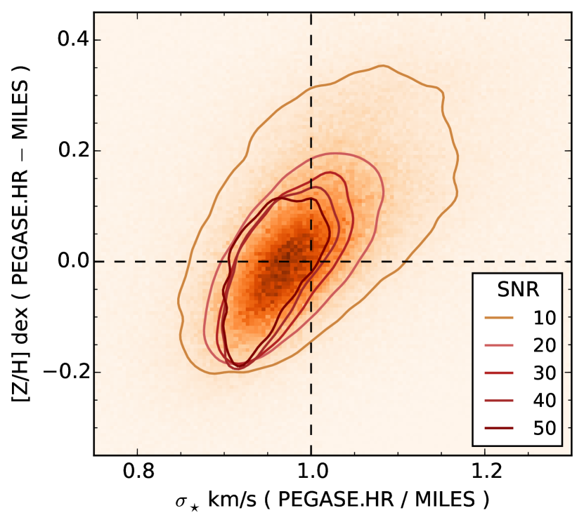
Figure 11.— Degeneracy between metallicity and velocity dispersion estimates shown as the ratio between velocity dispersions vs SSP metallicities obtained from the fitting of some 420,000 SDSS spectra using pegase.hr and MILES–PEGASE SSP models. The contours display the 1$\sigma$ values which correspond to the areas containing 68% galaxies with the spectra having signal-to-noise ratios within 20% of a displayed value. The number of galaxies for each contour ranges from $\sim$1800 (S/N=50) to $\sim$111,000 (S/N=10).

4.3. Emission line properties

4.3.1 Comparison of line fluxes with the MPA–JHU and OSSY catalogs and between the two techniques

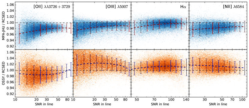
Figure 12.— Comparison of RCSED Gaussian emission line fluxes for 4 emission lines with the MPA–JHU (top row of plots) and OSSY (bottom row of plots) catalogs. The median and standard deviation of the distribution are shown by brown symbols with the error bars.

We compare a subset of our catalog containing measurements of emission line fluxes obtained from the parametric Gaussian fitting to the results from the MPA–JHU catalog distributed by the SDSS project (Brinchmann et al., 2004; Tremonti et al., 2004) and with the OSSY catalog (Oh et al., 2011). We used OSSY emission line measurements prior to the internal extinction correction. Given that the fluxes were computed using very similar methodologies with the main different corresponding to the subtraction of the underlying stellar population and the Galactic extinction correction techniques used, we expect a very good agreement for well detected emission lines. We directly compare fluxes of the [Oii] (3727 Å), [Oiii] (5007 Å), H$\alpha$, and [Nii] (6584 Å) emission lines for a sample of galaxies where they were detected at a level exceeding 10$\sigma$ (i.e. Flux/$\sigma($Flux$)>10$). The results are presented in Fig. 12. We obtain an excellent agreement with a systematic difference of less than 1% and the standard deviation of residuals of about 2% for the bright end of the H$\alpha$ flux distribution. At the faint end (10$\sigma$ detection), the systematic difference stays within 2% while the standard deviation grows to 3%. Hence, we conclude that our emission line fitting code works as expected and does not introduce any substantial systematic errors to flux measurements.

Compared to H$\alpha$, the H$\beta$ line is much more sensitive to the age of the stellar population being subtracted. In Appendix A we discuss the systematic errors of the H$\beta$ measurements as a function of the age mismatch. In case of faint emission lines, the systematics dominates the measurements if the age was determined incorrectly, and makes them useless for the emission line diagnostics.

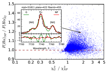
Figure 13.— Comparison of the H$\alpha$ fluxes obtained for the parametric (Gaussian) and non-parametric emission line profile fitting as a function of the $\chi^{2}$ ratio. An example profile decomposition is shown in the inset for an object with highly discrepant flux estimates.

The principal difference of our results with those published earlier is the non-parametric approach to the emission line fitting. For galaxies which exhibit some signs of nuclear activity, the Balmer lines fluxes derived non-parametrically significantly exceed the values obtained with the Gaussian fitting. In Fig. 13 we present the H$\alpha$ flux ratio between the two approaches. The inset contains the same Seyfert galaxy which we presented earlier in Fig. 5 and the arrow indicates its position in the diagram that suggests that its non-parametric H$\alpha$ flux estimate is about 20% higher than that obtained with the Gaussian profile fitting.

4.3.2 BPT diagrams and gas phase metallicities

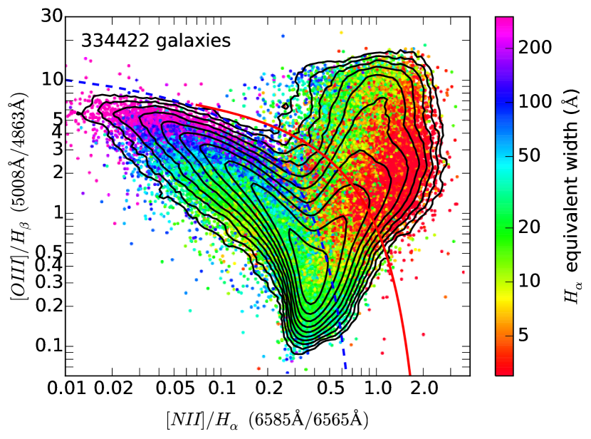
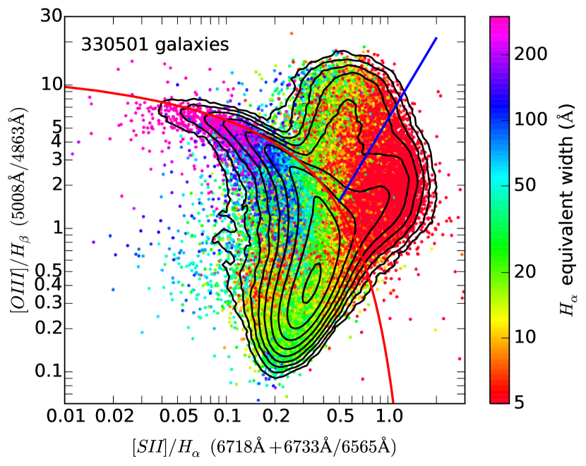
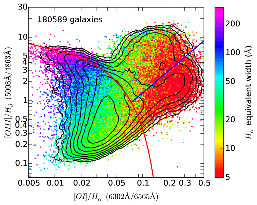
Figure 14.— Three flavors of a BPT diagram with the color coded $H_{\alpha}$ equivalent width. In each panel we display only those galaxies where all emission lines used in the corresponding plot have $S/N>3$. The contours correspond to the galaxy density smoothed with a moving average based on a 4$\times$4-pixels window. The number of galaxies kept in the sample is indicated inside each panel. The full and dashed lines correspond to starforming and transitional galaxies in Kewley et al. (2006).

In Fig. 14 we present three flavors of the BPT diagram which use different combinations of emission lines computed using the non-parametric fitting. The points are color-coded corresponding to the H$\alpha$ emission line EW. Cid Fernandes et al. (2010) proposed to use the H$\alpha$ EW to discriminate between Seyfert and LINER activity (instead of the traditionally used [Oiii]/H$\beta$ ratio), because H$\beta$ is often too weak to be detected and measured. We clearly see the bimodal distribution of non-starforming galaxies in the bottom two panels which corresponds to Seyfert galaxies (cloud to the top) and LINER/shockwave/post-AGB ionization (cloud to the bottom). The top panel displays the original BPT relation. The region between the red solid and the blue dashed lines defines “transitional” galaxies (Kewley et al., 2006) which we included in the calculation of metallicities in addition to the star forming galaxies located to the bottom left of the blue dashed line.

As we described above, RCSED includes gas phase metallicity measurements calculated with the Bayesian method implemented in the IZI software package with the Dopita et al. (2013) model grid, which uses all available emission lines in a spectrum; and a recent technique by Dopita et al. (2016) that relies on the [N/O] calibration and uses only 5 emission lines around H$\alpha$.

Kewley & Ellison (2008) demonstrated that different emission line calibrations yield largely inconsistent gas phase metallicity estimates when applied to the same input dataset with the differences reaching 0.7 dex (5 times). There is currently no consensus in the astronomical community about which calibrations produce more reliable metallicity estimates with arguments for both direct (Andrews & Martini, 2013) and indirect (López-Sánchez et al., 2012) methods. Gas and stellar metallicities also seem to strongly disagree (Yates et al., 2012). We notice, however, that all emission line calibrations result in the gas phase [O/H] mass–metallicity relations spanning much lower range of metallicities than that of stellar metallicities for a given galaxy stellar mass range. All gas metallicity relations saturate at high metallicities and the saturation occurs at different values (see e.g. fig. 10 in Andrews & Martini, 2013). The highest range of metallicities is covered by the calibration used by Tremonti et al. (2004) and provided in the MPA–JHU catalog.

In Fig. 15 we present the comparison of the Dopita et al. (2016) calibration with the MPA–JHU metallicities (blue shaded area) for 231,107 galaxies with the signal-to-noise ratios of H$\alpha$, [Nii], [Oii], and [Oiii] lines exceeding 10. The agreement is very good at $12+$[O/H]$<9$ dex with the standard deviation of the difference $0.08$ dex. At higher abundances Dopita et al. (2016) metallicities become slightly higher than those from the MPA–JHU dataset.

We ran the IZI metallicity determination code for a small sub-sample of 20,000 randomly selected starforming galaxies with high signal-to-noise emission lines (S/N$>$10) using all available grids of models and compared the derived metallicities with those obtained with the Dopita et al. (2016) calibration for the same galaxy sample. The only model grid that demonstrated a satisfactory agreement was that from Dopita et al. (2013). As expected, it also provides a satisfactory agreement with the MPA–JHU catalog (see Fig. 15, orange shaded areas) with the standard deviation of the difference $0.10$ dex.

In Fig. 16 we show the luminosity–metallicity relation (left panel) and the comparison of gas phase and SSP stellar metallicities (right panel) for the IZI–based determination using the Dopita et al. (2013) models (orange contours) and the Dopita et al. (2016) calibration (blue points). The mass–metallicity relation is well defined and we clearly see that the Dopita et al. (2013) model grid used in IZI yields a flatter shape than the more recent calibration (Dopita et al., 2016).

The comparison of gas phase and stellar metallicities reveal a substantial offset ranging from about 0.3 dex at solar stellar metallicities to 0.8 dex at the low end ([Fe/H]${}_{\mathrm{star}}=-1.1$ dex). Keeping in mind that stellar and gas phase metallicities might have different zero points and should not be directly compared to each other, the observed pattern is exactly what is expected due to the self enrichment of stellar populations happening in galaxies with extended star formation histories. The stars during their evolution form heavy elements which then get ejected into the ISM and recycled in the subsequent generations of stars, hence, increasing their metal abundances (see e.g. Matteucci, 1994). Therefore, younger generations of stars become more metal rich. SSP models probe mean stellar metallicities over the entire lifetime of a galaxy weighted with the stellar $M/L$ ratios and the star formation rate while the gas phase metallicity reflects the current chemical abundance pattern in the ISM enriched with metals, therefore, we expect to see the offset in metallicities. On the other hand, for the constant metal production rate per solar mass, the difference at low metallicities will be higher because the metallicity scale is logarithmic, therefore stellar metallicities should span a larger range of value compared to gas phase metallicities and the mass–metallicity relation slopes for gas will be shallower than that for stars.

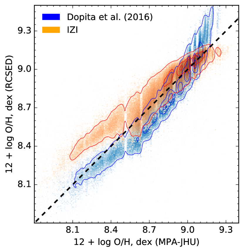
Figure 15.— Comparison of gas phase metallicities published in the MPA–JHU catalog (horizontal axis) to our measurements (vertical axis). The results of the IZI Bayesian technique are shown in brown and the measurements obtained with the Dopita et al. (2016) calibration are shown in blue.

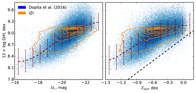
Figure 16.— Relation between a gas phase metallicity and a galaxy luminosity (left) and an SSP stellar metallicity (right). Blue dots and orange density contours display Dopita et al. (2016) and IZI metallicities correspondingly. The median and standard deviation of Dopita et al. (2016) measurements are shown by brown symbols with the error bars.

5. Catalog access: web-site and Virtual Observatory access interfaces

Efficient, convenient, and intuitive data access mechanisms and interfaces are essential for a complex project like RCSED. Therefore, we decided to build access interfaces for both interactive and batch access to the data.

RCSED includes several different data types (e.g. spectra and tabular data) and our access infrastructure (see Fig. 17) is organized to simplify their usage through different interfaces. The most natural way to access the catalog is by using the web application at http://rcsed.sai.msu.ru/. It provides a single-field google-style search interface where one can query the catalog by an object identifier, coordinates or object properties, e.g. select all galaxies with redshifts $z<0.1$ having red colors $g-r>1.5$. Every object in the sample has its own web page with the summary of all its properties, SED, spectral data available in the catalog, and image cutouts displaying the object at different wavelength provided by GALEX, SDSS, and UKIDSS surveys. An example of a spectrum summary plot presented on such web pages for every object is given in Fig. 4.

We developed an Application Programming Interface (API) to UKIDSS data, which allow us to extract image cutouts around an arbitrary position with a given box size in every filter. From cutout images in the JHK bands we generate a color composite image and display it in the object web-page. The API implemented in python is available for download from the project web-site. Another service we present is an interactive spectrum plotter implemented in JavaScript, our alternative to the SDSS spectrum plotter. It contains a number of value-added features, such as the display of best-fitting templates and identification of emission lines.

In addition to the custom web application, our data distribution infrastructure has the open source GAVO DaCHS data center suite in its core (see Fig. 17) which provides a set of VO data access mechanisms.

The data for SDSS spectra and their best-fitting SSP models are provided as FITS files that can be fetched by direct unique URLs. One can find a URL for every particular object spectrum file either in the object’s web page or by querying the provided IVOA Simple Spectral Access Protocol (SSAP) web service using object coordinates. The SSAP web service answers essentially with a list of spectra URLs and it is convenient to access programmatically or by using VO compatible client applications such as TOPCAT (Taylor, 2005), SPLAT-VO or VO-Spec which can directly load spectral data for further analysis by analyzing the SSAP web service query result.

For the ultimate flexibility of querying tabular catalog data, we provide a Table Access Protocol (TAP) web service. IVOA TAP is an access interface, which allows a user to query the entire relational database schema (see Fig. 18) using a powerful SQL-like language. It can be considered as an open source equivalent of the SDSS CasJobs service. Again, TAP web service can be used for script-based access as well as by using desktop VO applications. In particular, TOPCAT has a very useful TAP query dialogue with built-in help, query examples, syntax highlighting and given database schema assistance tools. We encourage our users to access the RCSED TAP web service through TOPCAT. We also note that our TAP service has a table upload capability, so that the user can upload his/her own tables and use it in subsequent SQL queries i.e. in join clauses, that is convenient for cross-identification of user provided object samples with the RCSED objects without the need of downloading our full catalog.

Below we give several query examples that are helpful to start using the RCSED database. More query examples and science case tutorials are provided on the project website http://rcsed.sai.msu.ru. Our TAP web service can be used for joining tables from the database schema specphot presented in Fig. 18, so that it is easy to retrieve a single table with the GalaxyZoo morphology, the photometric bulge+disk decomposition and the RCSED basic parameters combined for any galaxy of interest. An example of such a query to select all those data for a particular object would be:

SELECT
  r.*, g.*, s2.*
FROM
  specphot.rcsed AS r
  JOIN specphot.galaxyzoo AS g
    ON r.objid = g.objid
  JOIN specphot.simard_table2 AS s2
    ON r.objid = s2.objid
WHERE
  r.objid = 587731891649052703

Note that specphot prefix for table names corresponds to the name of the database schema where RCSED tables are stored. A query to retreive all data from the RCSED on galaxies, classified as ellipticals in GalaxyZoo is:

SELECT
  r.*
FROM
  specphot.rcsed AS r
  JOIN specphot.galaxyzoo AS g
    ON r.objid = g.objid
WHERE
  g.elliptical = 1

A query to select the data for a BPT (Baldwin et al., 1981) diagram for 10,000 galaxies with ${\rm S/N}>10$ in the corresponding line fluxes obtained with the Gaussian fitting looks like this:

SELECT
  TOP 10000
  f6550_nii_flx / f6565_h_alpha_flx AS BPT_x,
  f5008_oiii_flx / f4863_h_beta_flx AS BPT_y
FROM
  specphot.rcsed_lines_gauss
WHERE
  f6565_h_alpha_flx / f6565_h_alpha_flx_err > 10
  AND f5008_oiii_flx / f5008_oiii_flx_err > 10
  AND f4863_h_beta_flx / f4863_h_beta_flx_err > 10
  AND f6550_nii_flx / f6550_nii_flx_err > 10

Finally, all the catalog tables (see Fig. 18) are available for download as FITS tables from the project’s website for the offline use.

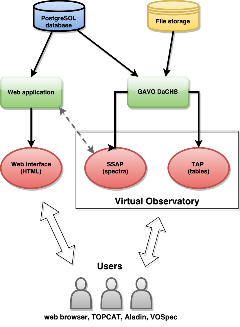
Figure 17.— Block diagram of the catalog data access infrastructure. Data are stored in the relational database (catalog tables and spectra metadata) and on the disk (FITS files with spectra and continuum models). They are accessed by applications (a custom web application and the GAVO DaCHS suite) which in turn expose several public access interfaces suitable for convenient queries and data retrieval by the multitude of user client programs, both VO-compatible and generic.

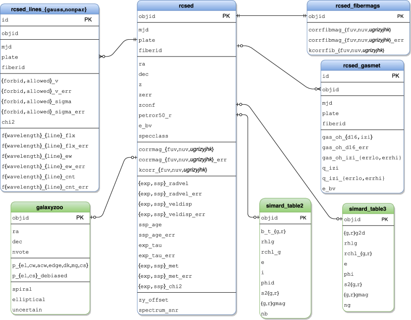
Figure 18.— The entity–relationship diagram for the tables in the catalog database. Blue color denotes original tables computed in RCSED, green color is for external datasets added to the database for convenience. Main table is rcsed which has a 1-to-1 relation to the rcsed_fibermags table by the primary key column objid,a 1-to-many (optional) relation to the rcsed_gasmet table with gas phase metallicity measurements, 1-to-many (optional) relations to rcsed_lines_gauss, rcsed_lines_nonpar tables with parametric (gauss) and non-parametric emission lines measurements. galaxyzoo, simard_table2 and simard_table3 datasets are all linked to the main table by the objid column and provide morphological classification and structural properties of galaxies from our sample using the data form Lintott et al. (2011) and Simard et al. (2011) respectively. All these tables are stored in specphot database schema, so the properly qualified table name is, for example, specphot.rcsed. We also note that all column names in the database are lowercase for homogeneity. Same schema and relationships applies to the distribution of RCSED in the form of FITS tables available for download from project’s website.

6. Summary

We presented a reference catalog of homogeneous multi-wavelength spectrophotometric information for some 800,000 low to intermediate redshift galaxies ($0.007<z<0.6$) from the SDSS DR7 spectroscopic galaxy sample with value-added data. For every galaxy we provide:

• a $k$-corrected and Galactic extinction corrected far-UV to NIR broad band SED for integrated fluxes compiled from the SDSS (optical), GALEX (UV), and UKIDSS (NIR) surveys

• a $k$-corrected and Galactic extinction corrected far-UV to NIR broad band SED for fluxes in circular 3-arcsec apertures that correspond to SDSS spectral apertures

• results of the full spectrum fitting of an SDSS spectrum using the nbursts technique that includes: (a) an original SDSS spectrum; (b) the best-fitting simple stellar population template in the wavelength range $3700<\lambda<6800$ Å and the best-fitting stellar population model with an exponentially declining star formation history in the wavelength range $3900<\lambda<6800$ Å; (c) estimates of stellar radial velocities, velocity dispersions, age, an exponential characteristic timescale for the star formation history, metallicities for two sets of stellar population models

• results of the emission line analysis using parametric (Gaussian) and non-parametric line profiles that include: (a) emission line fluxes corrected for the Galactic extinction; (b) estimates of the reddening inside a galaxy for star formation dominated systems derived from the observed Balmer decrement; (c) radial velocity offsets with respect to stars; (d) intrinsic emission line widths for the parametric fitting

• cross-match of a galaxy with third-party catalogs providing its structural parameters from the two-dimensional light profile fitting (Simard et al., 2011) and galaxy morphology by the Galaxy Zoo project (Lintott et al., 2008)

The catalog is fully integrated into the international Virtual Observatory infrastructure and available via a web application and as a Virtual Observatory resource providing IVOA TAP and IVOA SSAP interfaces in order to programmatically access tabular data and spectra correspondingly.

In addition to that, we presented best-fitting polynomial approximations for the red sequence shape in color–magnitude diagrams that include different colors, and mean colors for galaxies of 6 morphological types, from elliptical to late type spirals and irregulars and 3 luminosity classes (giants, intermediate luminosity, dwarfs).

Our catalog has already been used in several research projects that can be categorized into two groups: (i) statistical studies of galaxy properties; (ii) search and discovery of rare galaxies.

The first interesting result obtained with RCSED was the discovery of a universal 3-dimensional relation of NUV and optical galaxy colors and luminosities (Chilingarian & Zolotukhin, 2012). It also demonstrated that the integrated NUV$-$r color is a good proxy for a morphological type. The spectum fitting results for elliptical galaxies were later used in the re-calibration of the fundamental plane in SDSS (Saulder et al., 2013) which allowed us to compute redshift independent distances to early-type galaxies. Finally, we performed a calibration of near-infrared stellar $M/L$ ratios using optical colors and computed stellar masses for a new catalog of groups and clusters combining SDSS and 2MASS redshift survey data (Saulder et al., 2016). Our non-parametric emission line fitting results will be used to perform massive determinations of virial black hole masses in AGNs (Katkov et al. in prep). Other potential applications of statistical studies based on RCSED include but not limited to: environmental dependence of galaxy scaling relations and stellar population properties; connecting AGNs to stellar populations in galaxy centers; comparing different star formation rate indicators (e.g. emission line fluxes, UV and MIR photometry).

Thanks to the unique combination of photometric and spectral data as well as physical properties of galaxies derived from them, RCSED becomes an efficient search tool for rare or unique galaxies. Our dataset was used to discover and characterize massive compact galaxies at intermediate redshifts $0.2<z<0.8$ (Damjanov et al., 2013) which were thought to exist only in the early Universe ($z>1.5$) and measure their volume density (Damjanov et al., 2014). Then, using their fundamental plane positions, intermediate redshift compact galaxies were shown to be an extension of normal ellipticals to the compact regime (Zahid et al., 2015). Finally, it was demonstrated that some massive compact early-type galaxies actually stopped forming stars very recently (Zahid et al., 2016). We also used the universal UV–optical color–color–magnitude relation to define complex selection criteria and discover 195 previously considered extremely rare compact elliptical galaxies (Chilingarian & Zolotukhin, 2015). One can identify other obvious extragalactic rarities easily searchable with RCSED: post-starburst galaxies, candidate double-peaked AGNs, dwarf AGN hosts, “normal” galaxies with peculiarities detectable in multi-wavelength data such as ellipticals with NUV excess.

In the future, we anticipate to release intermediate and high redshift extensions of our catalog that will include the analysis of publicly available spectra from the Smithsonian Astrophysical Observatory Hectospec archive collected with the Hectospec multi-fiber spectrograph (Fabricant et al., 2005) the 6.5-m MMT and the DEEP2 galaxy redshift survey (Newman et al., 2013) made with the DEIMOS spectrograph at the 10-m Keck telescope. We also plan to expand the wavelength coverage by adding the all-sky infrared data from the Wide-field Infrared Survey Explorer (WISE) satellite (Wright et al., 2010). A major update to our catalog will be made with the full spectrophotometric fitting the entire sample using the nbursts+phot algorithm (Chilingarian & Katkov, 2012) and resolving star formation histories for about $10^{5}$ galaxies with high quality UV and NIR data.

Appendix A Systematics in emission line measurements due to stellar population template mismatch

Absorption lines of the hydrogen Balmer series contain important information about stellar population ages (Worthey, 1994), they become weaker when stars get older. At the same time, emission Balmer lines are used for the ISM diagnostic and star formation studies (Baldwin et al., 1981). For the vast majority of galaxies in our sample, we see relatively weak emission lines on top of a stellar continuum. Therefore, in order to accurately measure emission line fluxes, we need to precisely model stellar populations. Hence, when gas emission lines reside on top of a stellar continuum, any systematic uncertainty in the modelling of absorption lines will affect emission line measurements. Specifically, the age mismatch in the stellar population fitting will substantially bias Balmer line fluxes.

In order to quantify this effect, we performed the following procedure: (i) We selected 2,000 spectra from our sample with Balmer emission line intensities ranging from weak to strong based on their equivalent widths; (ii) we fitted those spectra using stellar population model grids fixing the SSP age to 2, 4, 8, and 16 Gyr; (iii) we measured emission line fluxes in the fitting residuals in these four sets of spectra; (iv) we compared them to emission line fluxes obtained for best-fitting stellar populations presented in our catalog.

In Fig. 19 we present our results. It is clear, that the age mismatch affects emission line fluxes for weak lines: The systematic errors grow when lines become weaker, and the difference between the best fitting and the fixed ages templates gets higher. When ages are underestimated by the fitting procedure (i.e. a galaxy is older than the age of a template), Balmer emission line fluxes are underestimated too. Because forbidden lines often used in the gas state diagnostics (e.g. [Nii] or [Oiii]) do not lie on top of strong age sensitive absorption features, their fluxes remain virtually unaffected, hence, moving a galaxy over the diagnostic plots (e.g. BPT) and potentially leading to the ionization mechanism misclassification.

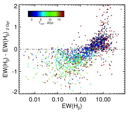
Figure 19.— The stellar population age mismatch effect on H$\beta$ flux measurements. The difference of the H$\beta$ EW computed using the best fitting SSP template and a template with the age fixed to 2 Gyr is plotted against the measured H$\beta$ EW for the best fitting SSP template. The age difference between the best fitting SSP age and 2 Gyr is color coded.

Appendix B Catalog compilation: SQL query

When selecting the core sample of galaxies we performed the following SQL query in the SDSS CasJobs service in the DR7 context (see details in Section 2.1):

SELECT
     p.objID, p.ra, p.dec,

     p.modelMag_u, p.modelMagErr_u, p.modelMag_g, p.modelMagErr_g,
     p.modelMag_r, p.modelMagErr_r, p.modelMag_i, p.modelMagErr_i,
     p.modelMag_z, p.modelMagErr_z,

     petroMag_u, petroMagErr_u, petroMag_g, petroMagErr_g,
     petroMag_r, petroMagErr_r, petroMag_i, petroMagErr_i,
     petroMag_z, petroMagErr_z,

     p.fiberMag_u, p.fiberMagErr_u, p.fiberMag_g, p.fiberMagErr_g,
     p.fiberMag_r, p.fiberMagErr_r, p.fiberMag_i, p.fiberMagErr_i,
     p.fiberMag_z, p.fiberMagErr_z,

     p.petroR50_u, p.petroR50Err_u, p.petroR50_g, p.petroR50Err_g,
     p.petroR50_r, p.petroR50Err_r, p.petroR50_i, p.petroR50Err_i,
     p.petroR50_z, p.petroR50Err_z,

     p.extinction_u, p.extinction_g, p.extinction_r, p.extinction_i, p.extinction_z,

     s.specObjID, s.mjd, s.plate, s.fiberID,
     s.z, s.zerr, s.zconf, s.objType, s.sn_0, s.sn_1, s.sn_2,
     (SELECT stripe FROM dbo.fCoordsFromEq(p.ra,p.dec)) AS stripe,
     s.specClass

INTO mydb.RCSED_SDSS
FROM PhotoObj AS p, SpecObj as s
WHERE
    s.bestObjid = p.objID
    AND s.z >= 0.007
    AND s.z < 0.6
    AND s.specClass IN (dbo.fSpecClass(’GAL_EM’), dbo.fSpecClass(’GALAXY’))

This query returned 800,311 rows with 12 duplicate objects for which SDSS SpecObj table contains 2 records despite it is documented to be clean from duplicates. We discard these duplicate spectra by keeping the record with higher S/N out of each pair of duplicates (and hence having e.g. better redshift estimate). From now we continue with the sample of 800,299 galaxies.

The coordinates of obtained galaxies were then uploaded to the GALEX CasJobs service and the following query was performed there in GALEXGR6Plus7 context:

SELECT
     sdss.objid,
     galex_objid,

     nuv_mag, nuv_magerr, fuv_mag, fuv_magerr,
     nuv_mag_aper_1, nuv_magerr_aper_1, nuv_mag_auto,
     fuv_mag_aper_1, fuv_magerr_aper_1, fuv_mag_auto,
     e_bv
INTO mydb.RCSED_SDSS_GALEX

FROM
     (
          SELECT
               s.objid,
               (SELECT objid FROM dbo.fGetNearestObjEq(s.ra, s.dec, 0.05)) AS galex_objid
          FROM
               mydb.RCSED_SDSS_coords AS s
     ) AS sdss
JOIN
     photoObjAll AS p
     ON sdss.galex_objid = p.objid

This query returned 485,996 rows.

Appendix C Catalog column descriptions

In Tables 4–8 we provide descriptions and metadata for columns of the original tables of RCSED, which are shown in blue in Fig. 18. The external datasets available in the RCSED database are described in the corresponding original papers (see the text for references).

This column information is identical for FITS tables distribution of the catalog, as well as when accessing the RCSED database through the Table Access Protocol, or using the catalog website http://rcsed.sai.msu.ru. For each column name in every table we give: (i) units (dash sign indicates that a column is dimensionless or units are not applicable to it); (ii) data type in the database convention in order to guide a user on the precisionm and puropse of a column; (iii) IVOA Unified Content Descriptor (UCD) that helps one to identify equivalent physical quantities available for comparison in the VO or to associate a column and its uncertainty; and (iv) human readable description of the column contents. When a table includes many similar columns as in the case of spectral lines properties in the rcsed_lines_gauss and rcsed_lines_nonpar database tables, we only give metadata for first group of columns in it and abridge the rest (Table 7 and Table 8). The complete list of emission lines included in our catalog and the column name prefixes in rcsed_lines_gauss and rcsed_lines_nonpar are given in Table 2.

Table 4Main catalog table (rcsed) columns metadata and descriptions.

Column	Units	Datatype	UCD	Description
objid	-	bigint	meta.id;meta.main	SDSS ObjID (unique identifier)
specobjid	-	bigint	meta.id	SDSS SpecObjID (unique identifier within spectral galaxies sample)
mjd	-	integer	time.epoch	MJD of observation
plate	-	smallint	meta.id	SDSS plate ID
fiberid	-	smallint	meta.id	SDSS fiber ID
ra	deg	double	pos.eq.ra;meta.main	RA (J2000) of galaxy
dec	deg	double	pos.eq.dec;meta.main	Dec (J2000) of galaxy
z	-	real	src.redshift	Galaxy redshift
zerr	-	real	stat.error;src.redshift	Uncertainty of galaxy redshift
zconf	-	real	stat.fit.param;src.redshift	SDSS $r$edshift confidence
petror50_r	arcsec	real	phys.angSize	SDSS $r$adius containing 50% of Petrosian flux
e_bv	mag	real	phot.color.excess	E(B-V) at this (l,b) from SFD98
specclass	-	smallint	src.spType	SDSS spectral classification
corrmag_fuv	mag	real	phot.mag;em.UV.FUV	Galactic extinction corrected total (Kron-like elliptical aperture) magnitude in GALEX $FUV$ filter
corrmag_nuv	mag	real	phot.mag;em.UV.NUV	Same as above for GALEX $NUV$ filter
corrmag_u	mag	real	phot.mag;em.opt.U	Galactic extinction corrected total (Petrosian) magnitude in SDSS $u$ filter
corrmag_g	mag	real	phot.mag;em.opt.B	Same as above for SDSS $g$ filter
corrmag_r	mag	real	phot.mag;em.opt.R	Same as above for SDSS $r$ filter
corrmag_i	mag	real	phot.mag;em.opt.I	Same as above for SDSS $i$ filter
corrmag_z	mag	real	phot.mag;em.opt.I	Same as above for SDSS $z$ filter
corrmag_y	mag	real	phot.mag;em.IR.J	Same as above for UKIDSS $Y$ filter
corrmag_j	mag	real	phot.mag;em.IR.J	Same as above for UKIDSS $J$ filter
corrmag_h	mag	real	phot.mag;em.IR.H	Same as above for UKIDSS $H$ filter
corrmag_k	mag	real	phot.mag;em.IR.K	Same as above for UKIDSS $K$ filter
corrmag_fuv_err	mag	real	stat.error;phot.mag;em.UV.FUV	Uncertainty of corrmag_fuv column
corrmag_nuv_err	mag	real	stat.error;phot.mag;em.UV.NUV	Uncertainty of corrmag_nuv column
corrmag_u_err	mag	real	stat.error;phot.mag;em.opt.U	Uncertainty of corrmag_u column
corrmag_g_err	mag	real	stat.error;phot.mag;em.opt.B	Uncertainty of corrmag_g column
corrmag_r_err	mag	real	stat.error;phot.mag;em.opt.R	Uncertainty of corrmag_r column
corrmag_i_err	mag	real	stat.error;phot.mag;em.opt.I	Uncertainty of corrmag_i column
corrmag_z_err	mag	real	stat.error;phot.mag;em.opt.I	Uncertainty of corrmag_z column
corrmag_y_err	mag	real	stat.error;phot.mag;em.IR.J	Uncertainty of corrmag_y column
corrmag_j_err	mag	real	stat.error;phot.mag;em.IR.J	Uncertainty of corrmag_j column
corrmag_h_err	mag	real	stat.error;phot.mag;em.IR.H	Uncertainty of corrmag_h column
corrmag_k_err	mag	real	stat.error;phot.mag;em.IR.K	Uncertainty of corrmag_k column
kcorr_fuv	mag	real	arith.factor;em.UV.FUV	K-correction for GALEX $FUV$ magnitude
kcorr_nuv	mag	real	arith.factor;em.UV.NUV	Same as above for GALEX $NUV$ magnitude
kcorr_u	mag	real	arith.factor;em.opt.U	K-correction for (Petrosian) SDSS $u$ magnitude
kcorr_g	mag	real	arith.factor;em.opt.B	Same as above for SDSS $g$ magnitude
kcorr_r	mag	real	arith.factor;em.opt.R	Same as above for SDSS $r$ magnitude
kcorr_i	mag	real	arith.factor;em.opt.I	Same as above for SDSS $i$ magnitude
kcorr_z	mag	real	arith.factor;em.opt.I	Same as above for SDSS $z$ magnitude
kcorr_y	mag	real	arith.factor;em.IR.J	Same as above for UKIDSS $Y$ magnitude
kcorr_j	mag	real	arith.factor;em.IR.J	Same as above for UKIDSS $J$ magnitude
kcorr_h	mag	real	arith.factor;em.IR.H	Same as above for UKIDSS $H$ magnitude
kcorr_k	mag	real	arith.factor;em.IR.K	Same as above for UKIDSS $K$ magnitude
exp_radvel	km/s	real	spect.dopplerVeloc.opt	Radial velocity (exp SFH)
exp_radvel_err	km/s	real	stat.error;spect.dopplerVeloc.opt	Radial velocity error (exp SFH)
exp_veldisp	km/s	real	phys.veloc.dispersion	Velocity dispersion (exp SFH)
exp_veldisp_err	km/s	real	stat.error;phys.veloc.dispersion	Velocity dispersion error (exp SFH)
exp_tau	Myr	real	time.age	Age (exp SFH)
exp_tau_err	Myr	real	stat.error;time.age	Age error (exp SFH)
exp_met	-	real	phys.abund.Z	Metallicity (exp SFH)
exp_met_err	-	real	stat.error;phys.abund.Z	Metallicity error (exp SFH)
exp_chi2	-	real	stat.fit.chi2	Goodness of fit (exp SFH)
ssp_radvel	km/s	real	spect.dopplerVeloc.opt	Radial velocity (SSP)
ssp_radvel_err	km/s	real	stat.error;spect.dopplerVeloc.opt	Radial velocity error (SSP)
ssp_veldisp	km/s	real	phys.veloc.dispersion	Velocity dispersion (SSP)
ssp_veldisp_err	km/s	real	stat.error;phys.veloc.dispersion	Velocity dispersion error (SSP)
ssp_age	Myr	real	time.age	Age (SSP)
ssp_age_err	Myr	real	stat.error;time.age	Age error (SSP)
ssp_met	-	real	phys.abund.Z	Metallicity (SSP)
ssp_met_err	-	real	stat.error;phys.abund.Z	Metallicity error (SSP)
ssp_chi2	-	real	stat.fit.chi2	Goodness of fit (SSP)
zy_offset	mag	real	phot.mag;arith.diff	Offset applied to UKIDSS magnitudes to correct for mismatch with SDSS ones
spectrum_snr	-	real	stat.snr	Signal-to-noise ratio of SDSS spectrum at 5500A (restframe) in the 20A box

Table 5Fiber magnitudes table (rcsed_fibermags) columns metadata and descriptions.

Column	Units	Datatype	UCD	Description
objid	-	bigint	meta.id;meta.main	SDSS ObjID (unique identifier)
corrfibmag_fuv	mag	real	phot.mag;em.UV.FUV	Galactic extinction corrected 3” aperture magnitude in GALEX $FUV$ filter
corrfibmag_nuv	mag	real	phot.mag;em.UV.NUV	Same as above for GALEX $NUV$ filter
corrfibmag_u	mag	real	phot.mag;em.opt.U	Galactic extinction corrected fiber (3” aperture) magnitude in SDSS $u$ filter
corrfibmag_g	mag	real	phot.mag;em.opt.B	Same as above for SDSS $g$ filter
corrfibmag_r	mag	real	phot.mag;em.opt.R	Same as above for SDSS $r$ filter
corrfibmag_i	mag	real	phot.mag;em.opt.I	Same as above for SDSS $i$ filter
corrfibmag_z	mag	real	phot.mag;em.opt.I	Same as above for SDSS $z$ filter
corrfibmag_y	mag	real	phot.mag;em.IR.J	Galactic extinction corrected 3” aperture magnitude in UKIDSS $Y$ filter
corrfibmag_j	mag	real	phot.mag;em.IR.J	Same as above for UKIDSS $J$ filter
corrfibmag_h	mag	real	phot.mag;em.IR.H	Same as above for UKIDSS $H$ filter
corrfibmag_k	mag	real	phot.mag;em.IR.K	Same as above for UKIDSS $K$ filter
corrfibmag_fuv_err	mag	real	stat.error;phot.mag;em.UV.FUV	Uncertainty of corrfibmag_fuv column
corrfibmag_nuv_err	mag	real	stat.error;phot.mag;em.UV.NUV	Uncertainty of corrfibmag_nuv column
corrfibmag_u_err	mag	real	stat.error;phot.mag;em.opt.U	Uncertainty of corrfibmag_u
corrfibmag_g_err	mag	real	stat.error;phot.mag;em.opt.B	Uncertainty of corrfibmag_g
corrfibmag_r_err	mag	real	stat.error;phot.mag;em.opt.R	Uncertainty of corrfibmag_r
corrfibmag_i_err	mag	real	stat.error;phot.mag;em.opt.I	Uncertainty of corrfibmag_i
corrfibmag_z_err	mag	real	stat.error;phot.mag;em.opt.I	Uncertainty of corrfibmag_z
corrfibmag_y_err	mag	real	stat.error;phot.mag;em.IR.J	Uncertainty of corrfibmag_y
corrfibmag_j_err	mag	real	stat.error;phot.mag;em.IR.J	Uncertainty of corrfibmag_j
corrfibmag_h_err	mag	real	stat.error;phot.mag;em.IR.H	Uncertainty of corrfibmag_h
corrfibmag_k_err	mag	real	stat.error;phot.mag;em.IR.K	Uncertainty of corrfibmag_k
kcorrfib_fuv	mag	real	arith.factor;em.UV.FUV	K-correction for 3” aperture GALEX $FUV$ magnitude
kcorrfib_nuv	mag	real	arith.factor;em.UV.NUV	Same as above for GALEX $NUV$ magnitude
kcorrfib_u	mag	real	arith.factor;em.opt.U	K-correction for fiber (3” aperture) SDSS $u$ magnitude
kcorrfib_g	mag	real	arith.factor;em.opt.B	Same as above for SDSS $g$ magnitude
kcorrfib_r	mag	real	arith.factor;em.opt.R	Same as above for SDSS $r$ magnitude
kcorrfib_i	mag	real	arith.factor;em.opt.I	Same as above for SDSS $i$ magnitude
kcorrfib_z	mag	real	arith.factor;em.opt.I	Same as above for SDSS $z$ magnitude
kcorrfib_y	mag	real	arith.factor;em.IR.J	K-correction for 3” aperture UKIDSS $Y$ magnitude
kcorrfib_j	mag	real	arith.factor;em.IR.J	Same as above for UKIDSS $J$ magnitude
kcorrfib_h	mag	real	arith.factor;em.IR.H	Same as above for UKIDSS $H$ magnitude
kcorrfib_k	mag	real	arith.factor;em.IR.K	Same as above for UKIDSS $K$ magnitude

Table 6Gas phase metallicity table (rcsed_gasmet) columns metadata and descriptions.

Column	Units	Datatype	UCD	Description
id		bigint	meta.id;meta.main	Primary key
objid		bigint		SDSS ObjID
mjd	d	integer	time.epoch	MJD of observation
plate		smallint	meta.id	SDSS plate ID
fiberid		smallint	meta.id	SDSS fiber ID
e_bv	mag	real	phot.color.excess	Intrinsic E(B-V)
gas_oh_d16		real	phys.abund.Z	Oxygen abundance of ionized gas (12 + log O/H) calculated using Dopita+16 calibration from Gaussian fit to emission lines
gas_oh_d16_err		real	phys.abund.Z	Error of oxygen abundance of ionized gas (12 + log O/H) calculated using Dopita+16 calibration from Gaussian fit to emission lines
gas_oh_izi		real	phys.abund.Z	Oxygen abundance of ionized gas (12 + log O/H) calculated using IZI calibration from Gaussian fit to emission lines
gas_oh_izi_errlo		real	stat.error;phys.abund.Z	Lower error of oxygen abundance of ionized gas (12 + log O/H) calculated using IZI calibration from Gaussian fit to emission lines
gas_oh_izi_errhi		real	stat.error;phys.abund.Z	Upper error of oxygen abundance of ionized gas (12 + log O/H) calculated using IZI calibration from Gaussian fit to emission lines
q_izi		real	phys.ionizParam.rad	Ionization parameter calculated using IZI calibration from Gaussian fit to emission lines
q_izi_errlo		real	stat.error;phys.ionizParam.rad	Lower error of ionization parameter calculated using IZI calibration from Gaussian fit to emission lines
q_izi_errhi		real	stat.error;phys.ionizParam.rad	Upper error of ionization parameter calculated using IZI calibration from Gaussian fit to emission lines

Table 7Gaussian fit to emission lines table (rcsed_lines_gauss) columns metadata and descriptions.

Column	Units	Datatype	UCD	Description
id		bigint	meta.id; meta.main	Primary key
objid		bigint	meta.id	SDSS ObjID
mjd	d	integer	time.epoch	MJD of observation
plate		smallint	meta.id	SDSS plate ID
fiberid		smallint	meta.id	SDSS fiber ID
forbid_v	km/s	real	phys.veloc	Velocity measured simultaneously in all forbidden lines
forbid_v_err	km/s	real	stat.error; phys.veloc	Uncertainty in the velocity measured simultaneously in all forbidden lines
forbid_sig	km/s	real	phys.veloc.dispersion	Velocity dispersion measured simultaneously in all forbidden lines
forbid_sig_err	km/s	real	stat.error; phys.veloc.dispersion	Uncertainty in the velocity dispersion measured simultaneously in all forbidden lines
allowed_v	km/s	real	phys.veloc	Velocity measured simultaneously in all allowed lines
allowed_v_err	km/s	real	stat.error; phys.veloc	Uncertainty in the velocity measured simultaneously in all allowed lines
allowed_sig	km/s	real	phys.veloc.dispersion	Velocity dispersion measured simultaneously in all allowed lines
allowed_sig_err	km/s	real	stat.error; phys.veloc.dispersion	Uncertainty in the velocity dispersion measured simultaneously in all allowed lines
chi2		real	stat.fit.chi2	Reduced goodness of fit
f3727_oii_flx	10-17 erg/s/cm2	real	phot.flux; spect.line	Flux from Gaussian fit to continuum subtracted data of [Oii] (3727 Å) line
f3727_oii_flx_err	10-17 erg/s/cm2	real	stat.error; phot.flux; spect.line	Uncertainty in the flux from Gaussian fit to continuum subtracted data of [Oii] (3727 Å) line
f3727_oii_cnt	10-17 erg/s/cm2/Å	real	phot.flux.density; spect.continuum	Continuum level at [Oii] (3727 Å) line center
f3727_oii_cnt_err	10-17 erg/s/cm2/Å	real	stat.error; phot.flux.density; spect.continuum	Uncertainty in the continuum level at [Oii] (3727 Å) line center
f3727_oii_ew	Å	real	spect.line.eqWidth	Equivalent width from Gaussian fit to continuum subtracted data of [Oii] (3727 Å) line
f3727_oii_ew_err	Å	real	stat.error; spect.line.eqWidth	Uncertainty in the equivalent width from Gaussian fit to continuum subtracted data of [Oii] (3727 Å) line
$\dots$	$\dots$	$\dots$	$\dots$	$\dots$

Table 8Non-parametric fit to emission lines table (rcsed_lines_nonpar) columns metadata and descriptions.

Column	Units	Datatype	UCD	Description
id		bigint	meta.id; meta.main	Primary key
objid		bigint	meta.id	SDSS ObjID
mjd	d	integer	time.epoch	MJD of observation
plate		smallint	meta.id	SDSS plate ID
fiberid		smallint	meta.id	SDSS fiber ID
forbid_v	km/s	real	phys.veloc	Velocity measured simultaneously in all forbidden lines
forbid_sig	km/s	real	phys.veloc.dispersion	Velocity dispersion measured simultaneously in all forbidden lines
allowed_v	km/s	real	phys.veloc	Velocity measured simultaneously in all allowed lines
allowed_sig	km/s	real	phys.veloc.dispersion	Velocity dispersion measured simultaneously in all allowed lines
chi2		real	stat.fit.chi2	Reduced goodness of fit
f3727_oii_flx	10-17 erg/s/cm2	real	phot.flux; spect.line	Flux from non-parametric fit to continuum subtracted data of [Oii] (3727 Å) line
f3727_oii_flx_err	10-17 erg/s/cm2	real	stat.error; phot.flux; spect.line	Uncertainty in the flux from non-parametric fit to continuum subtracted data of [Oii] (3727 Å) line
f3727_oii_cnt	10-17 erg/s/cm2/Å	real	phot.flux.density; spect.continuum	Continuum level at [Oii] (3727 Å) line center
f3727_oii_cnt_err	10-17 erg/s/cm2/Å	real	stat.error; phot.flux.density; spect.continuum	Uncertainty in the continuum level at [Oii] (3727 Å) line center
f3727_oii_ew	Å	real	spect.line.eqWidth	Equivalent width from non-parametric fit to continuum subtracted data of [Oii] (3727 Å) line
f3727_oii_ew_err	Å	real	stat.error; spect.line.eqWidth	Uncertainty in the equivalent width from non-parametric fit to continuum subtracted data of [Oii] (3727 Å) line
$\dots$	$\dots$	$\dots$	$\dots$	$\dots$

References

- Abazajian et al. (2009) Abazajian, K. N., Adelman-McCarthy, J. K., Agüeros, M. A., et al. 2009, ApJS, 182, 543
- Andrews & Martini (2013) Andrews, B. H., & Martini, P. 2013, ApJ, 765, 140
- Baldwin et al. (1981) Baldwin, J. A., Phillips, M. M., & Terlevich, R. 1981, PASP, 93, 5
- Becker et al. (1995) Becker, R. H., White, R. L., & Helfand, D. J. 1995, ApJ, 450, 559
- Bernardi et al. (2003) Bernardi, M., Sheth, R. K., Annis, J., et al. 2003, AJ, 125, 1849
- Blanc et al. (2015) Blanc, G. A., Kewley, L., Vogt, F. P. A., & Dopita, M. A. 2015, ApJ, 798, 99
- Blanton et al. (2003) Blanton, M. R., Hogg, D. W., Bahcall, N. A., et al. 2003, ApJ, 592, 819
- Blanton et al. (2005) Blanton, M. R., Schlegel, D. J., Strauss, M. A., et al. 2005, AJ, 129, 2562
- Brinchmann et al. (2004) Brinchmann, J., Charlot, S., White, S. D. M., et al. 2004, MNRAS, 351, 1151
- Bruzual & Charlot (2003) Bruzual, G., & Charlot, S. 2003, MNRAS, 344, 1000
- Cappellari & Emsellem (2004) Cappellari, M., & Emsellem, E. 2004, PASP, 116, 138
- Cappellari et al. (2006) Cappellari, M., Bacon, R., Bureau, M., et al. 2006, MNRAS, 366, 1126
- Chilingarian et al. (2007a) Chilingarian, I., Prugniel, P., Sil’chenko, O., & Koleva, M. 2007a, in IAU Symposium, Vol. 241, Stellar Populations as Building Blocks of Galaxies, ed. A. Vazdekis & R. R. Peletier (Cambridge, UK: Cambridge University Press), 175–176, arXiv:0709.3047