Identification of Jet-like events using a Multiplicity Detector

Abstract

We present a method for studying the detection of jets in high energy hadronic collisions using multiplicity detector in forward rapidities. Such a study enhances the physics scope of multiplicity detectors at forward rapidities in LHC. At LHC energies the jets may be produced with significant cross section in forward rapidities. A multi resolution wavelet analysis technique can locate the spatial position of jets due to its feature of space-scale locality. The discrete wavelet proves to be very effective in probing physics simultaneously at different locations in phase space and at different scales to identify jet-like events. The key feature this analysis exploits is the difference in particle density in localized regions of the detector due to jet-like and underlying events. We find that this method has a significant sensitivity towards detecting jet position and its size. The jets can be found with the efficiency and purity of the order of 46%.

1 Introduction

At Large Hadron Collider (LHC), with the large center-of-mass (CM) energy, multi-jet events may be produced with measurable cross-section in forward rapidities D0 . Typical 3-jets events arising from $qg\rightarrow qgg$ : $gg\rightarrow gg$ should appear in the ratio of 0.3:1 as discussed in 3jets . If the CM system has a boost either in +ve or in the -ve z-direction, the jets might be directed in the forward rapidity. For the partonic interaction of a low “x” gluon and the high “x” quark will lead to a jet in forward direction, where x is the fraction of momentum carried by the partons. One of the first measurement of inclusive jet production cross section in forward rapidities is performed in $p\bar{p}$ collision at $\sqrt{s}$ = 1.8 TeV with D0 detector at the Fermilab Tevatron D0 . The differential cross- section $d^{2}\sigma/(dE_{T}d\eta$) was measured upto $|\eta|$ $<$ 3, where $E_{T}$ is the transverse energy of the jet, $\sigma$ is the cross-section for jet production and $\eta$ is the jet pseudorapidity. The results are found to be in good agreement with next-to-leading order predictions from QCD nlo_jets and indicate a preference for certain parton distribution functions.

In pp collisions, dijet events will appear with jets lying back to back in azimuthal angle. In high energy experiments e.g. ALICE these may be easily studied using the central barrel detectors. However one may encounter events where the barrel detectors see two of more than two jets in an event where the toplogy may suggest a missing jet which may be in other part of the phase space (forward rapidity). If even the direction of such a missing jet can be found, more physics can be extracted from such an event. Jets in general produce particles which are confined to a cone and hence the spatial particle density within the jet region is expected to be very diferent compared to a normal event in pp collisions.

The aim of this study is to explore if this disticntion of localized high particle multilicity density can be exploited successfully to predict the jet direction or identify jet-like events. This study is aimed on the present high energy experiments STAR (at RHIC) and ALICE (at LHC). In the forward region of such experiments there are a set of charged particle detectors and a photon multiplicity detector. We have conducted this study using charged particle in the forward rapidity covering 2.3 $<$ $\eta$ $<$ 3.9.

In this paper, we have used a multiresolution analysis by discrete wavelet transformation (DWT) which has been successfully used in engineering, mathematics and computer science, astrophysics and multiparticle productions, DCC search Fang:1996ju ; Huang:1995tv ; Randrup:1997kt ; wavelet1 ; wavelet2 ; wavelet3 ; wavelet4 ; wavelet5 . In our study, we demonstrate that the DWT proves to be very useful in identifying jet-like events in terms of their position and size. There is no information loss due to completeness and orthogonality of the DWT basis. Also the wavelet transformation has advantages over traditional Fourier methods in analyzing physical situations where the signal contains discontinuities and sharp spikes. We have applied the wavelet transformation to the data of the PYTHIA pythia Monte Carlo simulation generated for p-p collisions at $\sqrt{s}$ = 7 TeV.

2 Model description

The simulation study is carried out using PYTHIA6 pythia event generator version 6.4. To make the results more realistic, we have applied a detetor response of such a multiplicity detector with typical values of efficiency and purity 60%. We have generated two sets of data, one for “minimum bias” and other for “jets” in pp collisions at $\sqrt{s}$ = 7 TeV. Since we are using charged particles in our study, the magnetic field could have significant effect and thus the study is also extended by incorporating field ON and OFF conditions.

The di-jet events are generated without any initial and final state radiations and at least one of the jets is allowed to fall in the forward rapidities (2.3 $<$ $\eta$ $<$ 3.9). The jet transverse energy is taken as $E_{T}$ $>$ 20 GeV . A typical distribution in $\eta$ - $\phi$ plane of particles from a jet event after putting a transverse momentum ($p_{T}$) threshold of 2 GeV/c on the produced particles is shown in Fig. 1. Fig. 2 shows particle density distribution for minimum bias (MB) and jet events in $\eta$ coverage, 2.3 $<\eta<$ 3.9 for four particular $\eta$ - $\phi$ bins at $\sqrt{s}$ = 7 TeV. These bins are the one where we allowed the jet to fall on. The multiplicity distribution for jets is fitted with double Negative Binomial Distribution (NBD) function and that for minimum bias is single NBD fit. The double NBD is needed to account for two types of particle production processes, one due to non-jet (soft processes) and other due to jets (hard processes).

Throughout this paper, the generated level result are named as MC truth and after applying detector response as Digits.

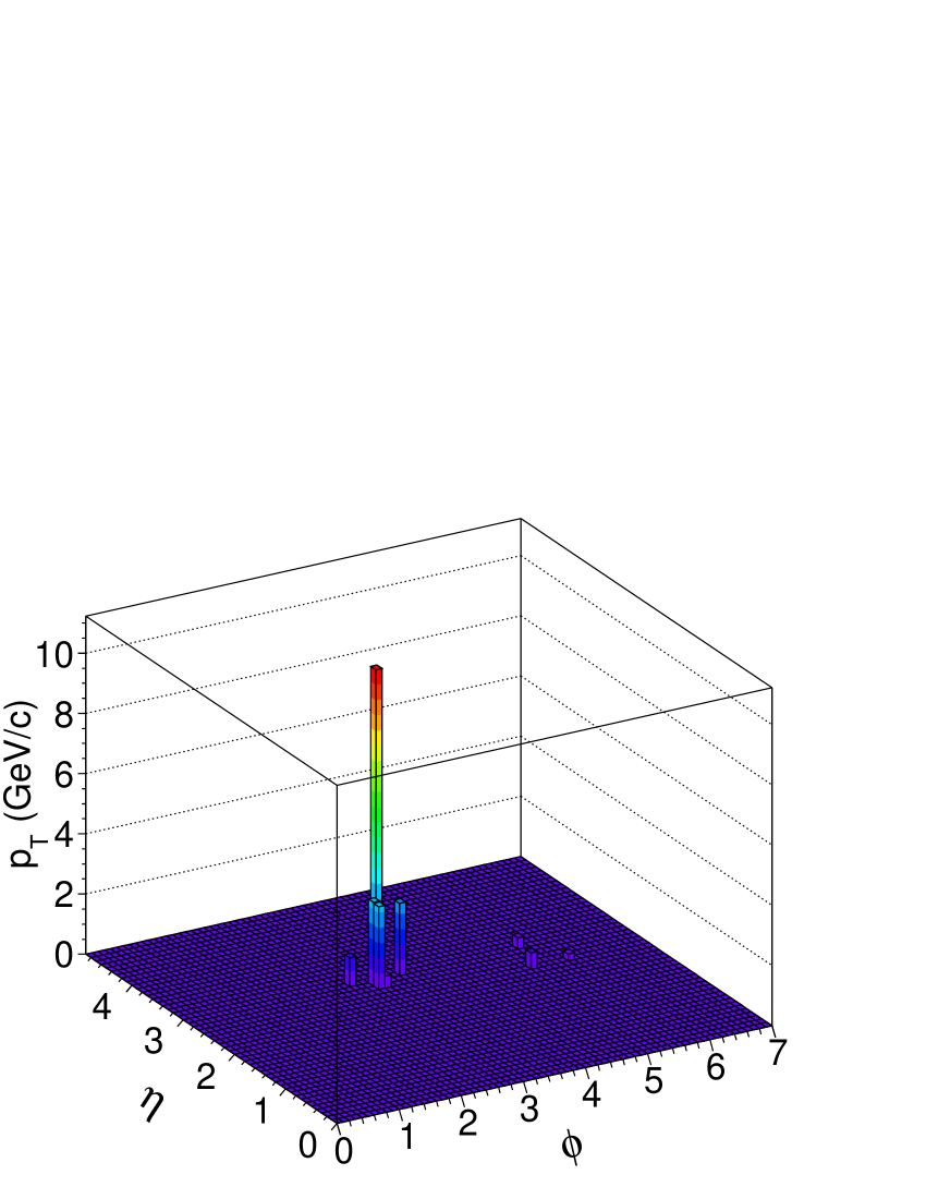
Figure 1: A typical PYTHIA simulated jet event of jet $E_{T}$ $>$ 20 GeV falling on forward rapidity (2 $<$ $\eta$ $<$ 4) in p-p collisions at $\sqrt{s}$ = 7 TeV.

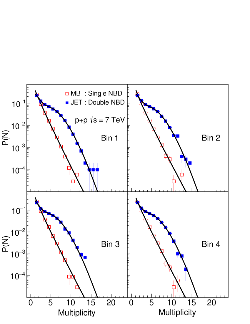
Figure 2: Multiplicity distribution for minimum bias (red marker) and jet events (blue marker) in four particular $\eta-\phi$ bins in p-p collisions at $\sqrt{s}$ = 7 TeV from MC truth.

3 A multi-resolution discrete wavelet technique

A discrete wavelet transform (DWT) is any wavelet transform for which the wavelets are discretely sampled. The DWT generalizes the standard Fourier analysis. We have performed our study with the idea of multiresolution analysis by using the well known Haar wavelet. For an input represented by a list of $2^{n}$ numbers, the Haar wavelet transform may be considered to simply pair up input values, storing the difference and passing the sum. This process is repeated recursively, pairing up the sums to provide the next scale: finally resulting in $2^{n}-1$ differences and one final sum. For the mathematical illustration, we consider a one-dimensional phase-space, described by the dimensionless variable $x$ in the interval $[0,1]$. We can divide this phase space in $2^{j}$ bins of size $\Delta x$ = $1/2^{j}$, where $j$ is a positive integer $j<j_{max}$, with $j_{max}$ corresponding to the finest resolution that can be attained. Let us consider a function $f(x)$ represents any observable on this interval such that

$$f^{(j)}(x)=\sum_{k=0}^{2^{j}-1}f_{k}^{j}\,\phi_{k}^{j}(x)$$ (1)

where $\phi_{k}^{j}(x)$ is given by

$$\phi^{j}_{k}(x)=\left\{\begin{array}[]{ll}1&k/2^{j}\leq x<(k+1)/2^{j}\\ 0&{\rm otherwise}\end{array}\right.\,.$$ (4)

$f_{k}^{j}(x)$ is the value of $f(x)$ in the $k^{th}$ bin. The family of bin bin functions $\phi^{j}_{k}(x)$ can be rewritten as the translations and dilation of a single function $\phi(x)$, called the mother function:

$$\phi^{n}_{m}(x)=\phi(2^{n}x-m)\,,$$ (5)

where, in the present case, $\phi(x)$ is the top-hat function.

In Eq. 5, the index $j$ denotes the resolution scale and $k$ the position at scale $j$. In the multiresolution analysis the sample function $f(x)$ can be find at various scales. For example, to find the structure at lower scale one can replace two adjacent bins $2k$ and $2k+1$ by a single bin of size $2\Delta x=1/2^{j−1}$ and corresponding bin function is given by

$$\phi^{j-1}_{k}(x)=\phi^{j}_{2k}(x)+\phi^{j}_{2k+1}(x)\,,$$ (6)

In the new bin $k$, by defining the value $f^{j-1}_{k}$ of the function as the average of the values in the previous smaller bins:

$$f^{j-1}_{k}=\frac{1}{2}(f^{j}_{2k}+f^{j}_{2k+1})\,.$$ (7)

The resulting sample function at scale $j-1$ is given by:

$$f^{(j-1)}(x)=\sum_{k=0}^{2^{j-1}-1}f^{j-1}_{k}\,\phi^{j-1}_{k}(x)\,.$$ (8)

$f^{j-1}_{k}$’s are called the mother function coefficients (MFCs) and the Eq. 8 express the mother function representation of the distribution $f(x)$ at scale $j-1$. This procedure can be repeated from the finest resolution scale $j_{max}$ to the lowest one $j=0$.

In the above procedure, another information that can be encoded is the difference $\tilde{f}^{(j-1)}(x)\equiv f^{(j)}(x)-f^{(j-1)}(x)$ and similarly can be represented as:

$$\tilde{f}^{(j-1)}(x)=\sum_{k=0}^{2^{j-1}-1}\tilde{f}^{j-1}_{k}\,\psi^{j-1}_{k}(x)\,,$$ (9)

where the $\psi^{j-1}_{k}$’s are called father function coefficients (FFCs) and given by:

$$\psi^{j-1}_{k}(x)=\phi^{j}_{2k}(x)-\phi^{j}_{2k+1}(x)\,.$$ (10)

The FFCs can be obtained by the operation of translations and dilations $\psi^{j}_{k}(x)=\psi(2^{j}x-k)$.

The FFCs in Eq. 9 are related to MFCs at previous scale $j$ as

$$\tilde{f}^{j-1}_{k}=\frac{1}{2}(f^{j}_{2k}-f^{j}_{2k+1})\,.$$ (11)

The FFCs at a given scale $j$ measure the variation of the sampled distribution $f$ between two adjacent bins.

To identify jet-like events, we have divided ($\eta-\phi$) region in both the physical space and scale space. The Haar basis is easy to visualize but not localized in scale space as the top-hat function is discontinuous. The simplest wavelet which is localized both in space and in scale is often called D4-wavelet D4_wavelet . Througout our analysis we have used D4-wavelet to investigate the scale dependence of multiplicity fluctuations.

In our analysis the input is the multiplicity in different $\eta$ and $\phi$ coverages. We have divided the accesible space in 16, $\eta-\phi$ bins (4 bins in $\eta$ in the range $2.3<\eta<3.9$ and 4 bins in $\phi$ in the range $0<\phi<2\pi$ ) and measure the multiplicity in each bin. So in total we have a input column matrix of $2^{4}$ dimension. The wavelet transformation give us the bin to bin fluctuation, in our case multiplicity fluctuations, in the form of wavelet coefficients (FFCs). In the next steps it sums up the bins and again calculates the coefficients and so on till it reaches the step where the only difference between last two bins remain.

In Minimum Bias case, we expect the multiplicity distribution over many events would be uniform in all the bins which will result in no or very less multiplicity fluctuations and hence wavelet coefficients approach to a small value. But in case of jet events, most of the particle in an event will be localized in a single or two bins which will results in higher fluctuations and wavelet coefficients attain higher and higher values. At a level or bin size in $\eta-\phi$, where the values of the fluctuation coefficients are higher gives us an estimate of the size of the jet.

4 Results

Using wavelet transformations, we obtain the first father coefficients and plot these coefficients for MB as well as jet-events and try to quantify the results. In Fig. 3 FFC distributions in different scales from MC truth are plotted. From the plots, a clear difference in FFCs distribution for MB and jet events are observed. The distribution is broader for jet-events sample as the fluctuations are large in these events. Also the broadening of FFCs distribution is large for scale J=2. The FFCs at a given scale carry information about the degree of fluctuations at higher scales. Due to completeness and orthogonality of the DWT basis, there is no information loss at any scale. Broader FFC distribution reflects more bin-to-bin multiplicity fluctuations, reflecting a jet-like behaviour. The scale describes the size of the jets on the detector. Fig. 4 shows the FFC distributions in different scales from Digits and the similar behaviour is observed as in case of MC truth. In order to quantify the analysis, we introduced a parameter $\xi$, called as strength parameter.

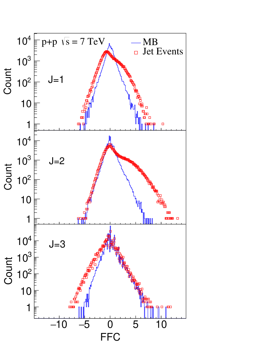
Figure 3: FFCs distribution for scale J=1, 2, 3 in p-p collisions at $\sqrt{s}$ = 7 TeV from MC truth. The jet events have jet $E_{T}$ $>$ 20 GeV.

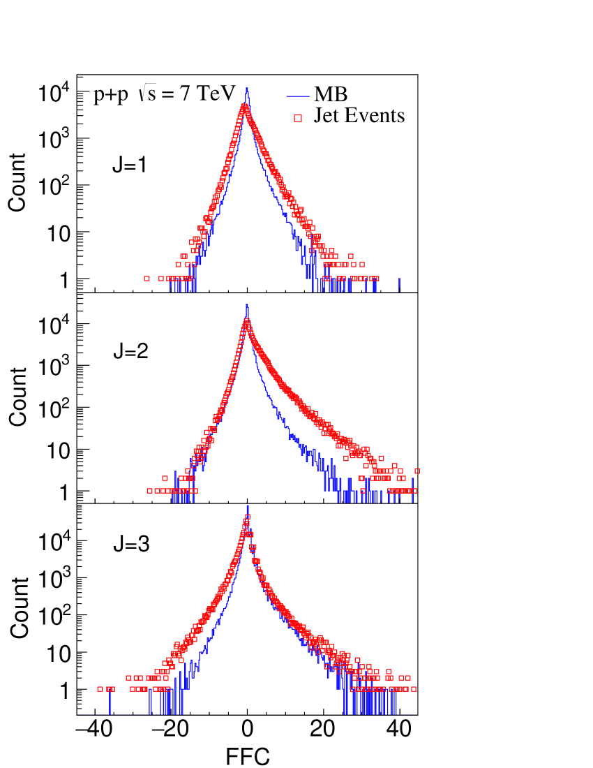
Figure 4: FFCs distribution for scale J=1, 2, 3 in p-p collisions at $\sqrt{s}$ = 7 TeV from Digits. The jet events have jet $E_{T}$ $>$ 20 GeV.

4.1 Strength parameter

In order to quantify the results and obtaining a cut to select jet like events, we introduce a strength parameter $\xi$. The value of strength parameter ($\xi$) is given by :

$$\xi=\frac{\sigma^{2}_{jet}-\sigma^{2}_{mb}}{\sigma_{mb}}\\$$ (12)

where $\sigma_{jet}$ and $\sigma_{mb}$ are widths of the FFCs distributions for jets and MB events respectively.

The parameter $\xi$, simply determines the deviation from normal distribution. Figure 5 shows the variation of $\xi$ with scale parameter J. We can see the variation is similar in both MC truth and digits level, but the values are little lower at digits level. This suggests the jet-like signal remains after passing through detector response. The maximum value of strength parameter is for J=2.

The results shown so far are for an ideal situation with full jet event sample. Now we consider a more realistic scenario of mixing the MB sample with different percentage of jet-events selected randomly and repeat the same analysis. We have studied seven such samples with jet event percentage: $1\%$, $5\%$, $10\%$, $20\%$, $30\%$, $40\%$ and $50\%$. Strength parameters is extracted for samples with different jet events percentage and plotted in Figure 6. The figure shows the strength parameter increases with increasing percentage of jet events. However the magnitude of strength is higher for MC truth than Digits. In Figure 7 strength parameter is plotted against the scale J=1, 2, 3 and the magnitude is higher for J=2 both for MC truth and Digits.

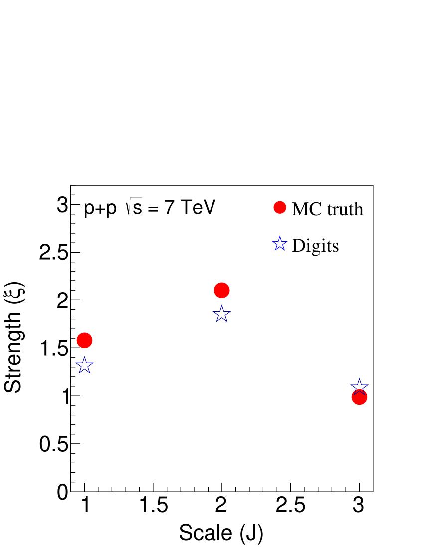
Figure 5: Strength ($\xi$) vs. scale parameter (J) in p-p collisions at $\sqrt{s}$ = 7 TeV from MC truth and Digits.

4.2 Model comparison

It is important here to check for any model dependence of present analysis. For this we have carried out the analysis with another event generator PHOJET phojet . The FFCs distribution for events generated from PHOJET are compared to those from PYTHIA6 pythia . Figure 8 shows the FFCs distribution for both the models for different scales. From the figure it is clear that there is very good agreement in the models and hence our results are model independent.

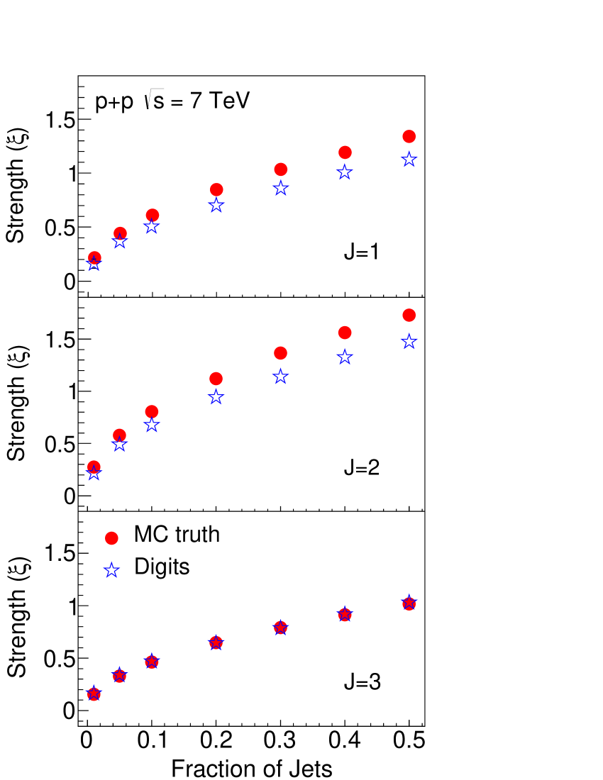
Figure 6: Strength ($\xi$) vs. fraction of jet events mixed in MB sample in p-p collisions at $\sqrt{s}$ = 7 TeV from MC truth and Digits.

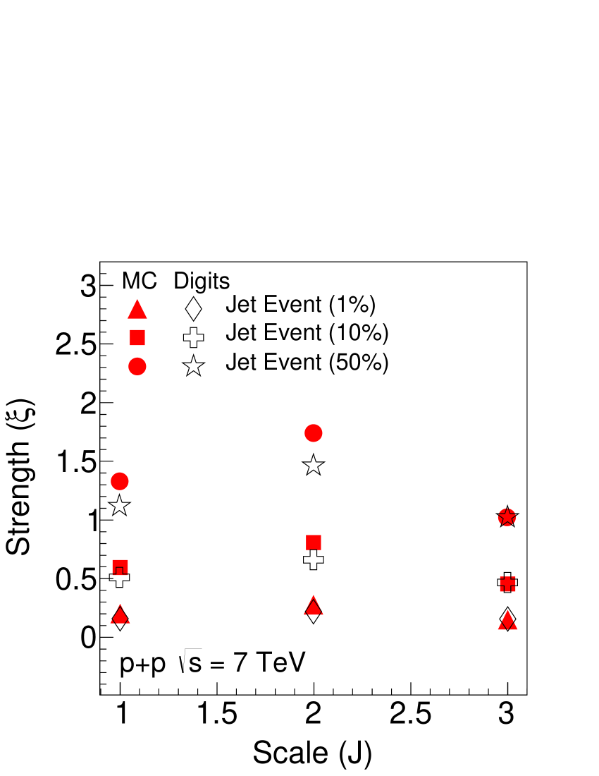
Figure 7: Strength ($\xi$) vs. scale parameter with different jet percentage in p-p collisions at $\sqrt{s}$ = 7 TeV from MC truth and Digits.

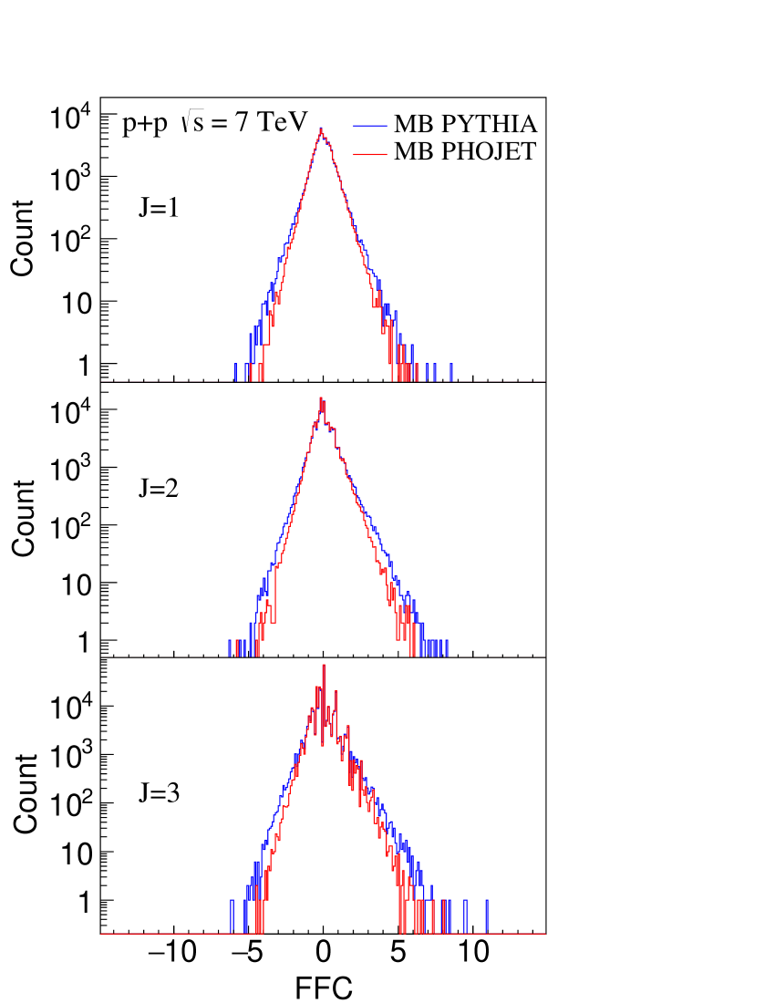
Figure 8: FFCs distribution in PYTHIA6 and PHOJET for scale J = 1, 2, 3 in p-p collisions at $\sqrt{s}$ = 7 TeV for MC truth.

4.3 Energy dependence

Figure 9 shows the strength parameter dependence on jet transverse energy for scale J=1, 2, 3 for MC truth and Digits. We have generated four events sample with jet $E_{T}$ ranging; 20-30 GeV, 30-40 GeV, 40-60 GeV and 20-100 GeV. From the figure we can see that the magnitude of $\xi$ is highest for jet $E_{T}$ = 40-60 GeV i.e. for high jet $E_{T}$ case.

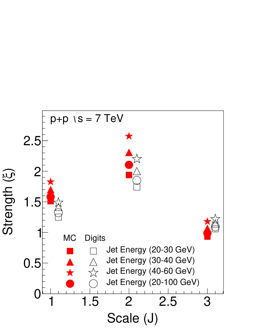
Figure 9: Strength ($\xi$) vs. scale parameter for different jet transverse energies in p-p collisions at $\sqrt{s}$ = 7 TeV from MC truth and Digits.

4.4 Efficiency, purity of selecting jet like events

Efficiency and purity of selecting jet-like events in a multiplicity detector is calculated by applying different rms cuts from normal FFCs distribution on a sample of mixed MB+jet events with $50\%$ jets. The efficiency and purity are defined as :

$$Efficiency=\frac{N_{j}}{N_{ja}}$$ (13)

$$Purity=\frac{N_{j}}{N_{jlike}}$$ (14)

where, $N_{j}$ = No. of jet events identified, $N_{ja}$ = No. of jet events added in the MB sample and $N_{jlike}$ = No. of jet like events. Figures 11 $\&$ 11 show the variation of efficiency / purity with the rms cuts obtained from the FFCs distribution of MB events for MC truth and Digits respectively. For a cut of 3 times the rms of FFCs distribution of MB events the efficiency and purity values are about 46$\%$.

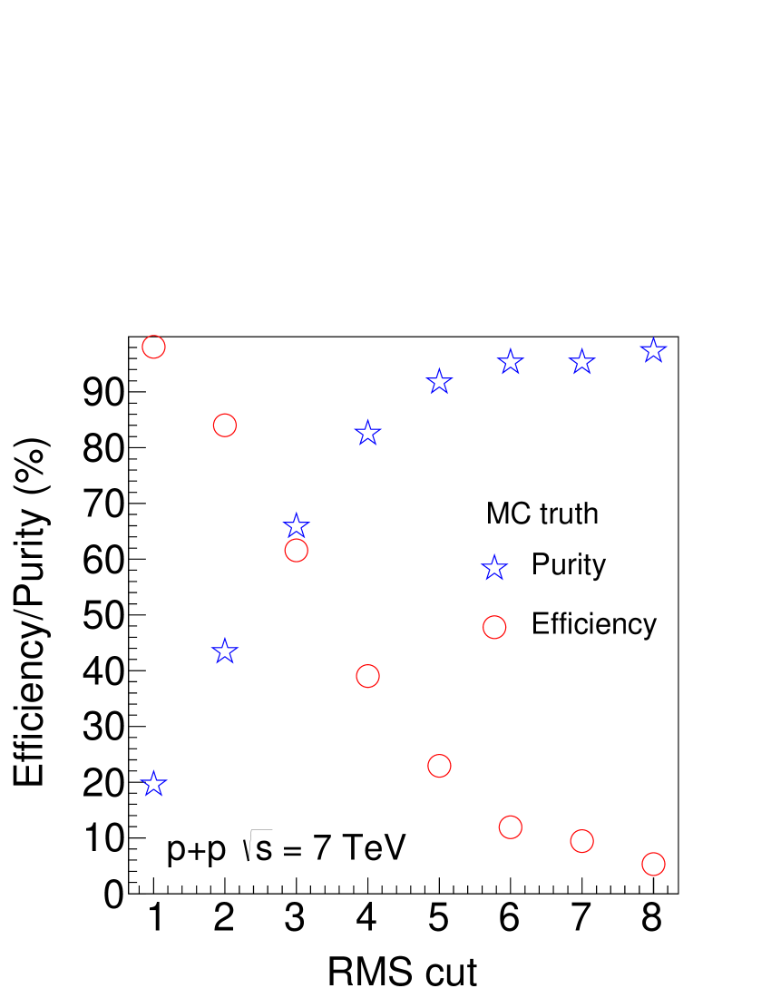
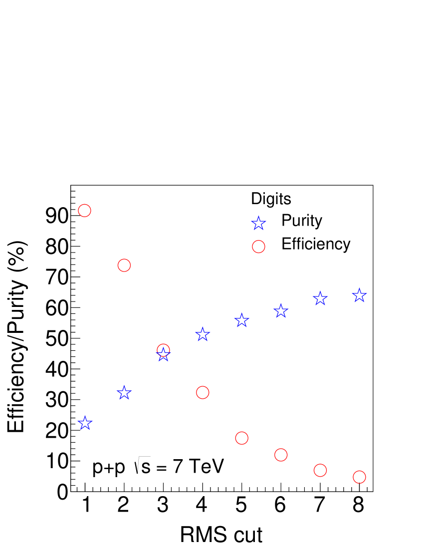
Figure 10: Efficiency, Purity vs. rms cut on MB FFCs distribution at $\sqrt{s}$ = 7 TeV from MC truth.

Figure 11: Efficiency, Purity vs. rms cut on MB FFCs distribution at $\sqrt{s}$ = 7 TeV from Digits.

5 Summary

We have reported a multi-resolution analysis technique to identify jet-like events in a multiplicity detector at LHC energies. The analysis is carried out using charged particle multiplicities. The observation of jet-like events can be used to tag 3-jet events in ALICE at LHC. The multi-resolution simulation study shows the good sensitivity towards selecting jet-like events in the forward multiplicity detector. The value of $\xi$ is 0.22, 0.65 & 1.42 for event samples with 1%, 10% and 50% jet-like events respectively. A $\xi$ value of zero would have indicated no sensitivity of the method towards identification of jet-like events. Such an analysis can be carried out in real data in future with p-p collisions at 0.9, 2.76, 7, 8 and 13TeV data collected by ALICE.

References

- (1) B. Abbott et al. (D0 Collaboration), Phys. Rev. Lett. 86, 1707 (2001).
- (2) K. Makhshoush and C. J. Maxwell, Phys. Lett. B 212 (1988).
- (3) W. T. Giele, E. W. N. Glover and D. A. Kosower, Phys. Rev. Lett. 73, 2019 (1994).
- (4) L. Z. Fang and J. Pando, arXiv:astro-ph/9701228.
- (5) Z. Huang, I. Sarcevic, R. Thews and X. N. Wang, Phys. Rev. D54, 750 (1996).
- (6) J. Randrup and R. L. Thews, Phys. Rev. D56, 4392 (1997).
- (7) X. N. Wang, Phys. Rev. D43, 104 (1991); X. N. Wang and M. Gyulassy, Phys. Rev. D44, 3501 (1991).
- (8) R. J. Adler, in“The Geometry of Random Field”, Wiley, New York (1981).
- (9) B. Mohanty et al., Int. J. Mod. Phys. A19, 1453 (2004).
- (10) B. Mohanty and J. Serreau, Phys. Rept. 414, 263 (2005).
- (11) A. Masuda, S. Yamamoto and A. Sone, JSME International Journal C, 40-4, 630 (1997).
- (12) I. Daubechies, in Ten Lectures on Wavelets, Society for Industrial and Applied Mathematics (SIAM), Philadelphia (1992).
- (13) T. Sjostrand, Comput. Phys. Commun. 82, 74 (1994); T. Sjostrand, S. Mrenna and P. Z. Skands, JHEP 0605, 026 (2006).
- (14) R. Engel, J. Ranft, S. Roesler, Phys. Rev. D 52, 1459 (1995).