Effect of anisotropy on generalized Chaplygin gas scalar field and its interaction with other dark energy models

Abstract

Abstract

In this work, we establish a correspondence between the interacting holographic, new agegraphic dark energy and generalized Chaplygin gas model in Bianchi type I universe. In continue, we reconstruct the potential of the scalar field which describes the generalized Chaplygin cosmology. Cosmological solutions are obtained when the kinetic energy of the phantom field is order of the anisotropy and dominates over the potential energy of the field. We investigate observational constraints on the generalized Chaplygin gas, holographic and new agegraphic dark energy models as the unification of dark matter and dark energy, by using the latest observational data. To do this we focus on observational determinations of the expansion history $H(z)$. It is shown that the HDE model is better than the NADE and generalized Chaplygin gas models in an anisotropic universe. Then, we calculate the evolution of density perturbations in the linear regime for three models of dark energy and compare the results $\Lambda$CDM model. Finally, the analysis shows that the increase in anisotropy leads to more correspondence between the dark energy scalar field model and observational data.

keywords: Anisotropic universe, Holographic dark energy, New agegraphic dark energy, Interacting dark energy, Generalized Chaplygin gas.

I Introduction

A series of astronomical observations over the past decade indicate that our universe confirms a state of accelerated expansion 1 ; 2 . Present observational cosmology has provided enough evidence in favour of the accelerated expansion of the universe 3 ; 4 ; 5 ; 6 ; 8 . There exists some unknown energy, which is called dark energy (DE), to realize the accelerated expansion. A cosmological constant ($\Lambda$) has effective equal pressure to minus its energy density (equation of state $\omega_{\Lambda}=-1$) consistent with preliminary measurements, but in supersymmetric theories the most natural scale for $\Lambda$ is at least as large as 100 GeV. So far it also so-called $\Lambda$CDM, which provides an excellent fit to a wide range of astronomical data. As regards, the $\Lambda$CDM model confronts problems, which are namely “fine-tuning” and “cosmic coincidence” 91 ; 92 . Other the simplest extension of $\Lambda$ is the DE with a constant $w$, which is the corresponding cosmological model so-called that $wC$DM model 93 ; 94 . Recent reviews 10 ; 11 ; 12 ; 13 are useful for a brief knowledge of DE models. In recent years, the holographic DE (HDE) has been studied as a possible candidate for DE. It is commonly believed that the holographic principle 14 ; 15 ; 16 is just a fundamental principle of quantum gravity too. Holographic principle is illuminated by investigations of the quantum property of black holes. In this sense, the number of freedom’s degrees of a physical system should be finite and scale with its bounding area rather than with its volume. It should be constrained by an infrared cut-off 17 . According to 17 the energy contained in a region of size $L$ must not exceed the mass of a black hole of the same size, which means, in terms of energy density, $\rho_{\Lambda}\leq L^{-2}$. Based on this idea, 18 proposed the HDE model, where the infrared cutoff is taken to be the size of event horizon for DE. More details about the HDE was studied by many authors 19 ; 20 ; 21 ; 22 ; 23 ; 24 ; 25 .
Another proposal to explore the nature of DE within the framework of quantum gravity is the agegraphic DE (ADE) 26 . This model takes into account the Heisenberg uncertainty relation of quantum mechanics together with the gravitational effect in general relativity. The ADE model considers spacetime and matter field fluctuations responsible for DE. However, the ADE model might contain an inconsistency 27 . So to overcome this problem, which after the ADE model, the authors 28 proposed an alternative model of DE, is namely the “new agegraphic DE” (NADE). The NADE models have been studied in plentiful detail by 29 ; 30 .
It was purposed the use of some perfect fluid with an equation of state and called it as Chaplygin gas (CG) 31 . The CG is one of the candidate of DE models to explain the accelerated expansion of the universe. The striking features of CG DE is that it can be assumed as a possible unification of DM and DE. The CG plays a duplex role at different epoch of the history of the universe: it can be as a dust-like matter in the early time (i.e. for small scale factor $a$), and as a cosmological constant at the late time. Bertolami et al. 32 have found the generalized Chaplygin gas (GCG) which is better fit for latest Supernova data. After the GCG was introduced, the new model of CG which is called modified CG (MCG) was proposed. An interesting feature of MCG is its ability to explain the evolution of the universe from radiation to $\Lambda$CDM 33 ; 34 . On the other hand, it is considered the reconstructing between the scalar field and the DE models, which is the case, for example, holographic quintessence 35 , holographic tachyon 36 , interacting new agegraphic tachyon, K-essence and dilaton 37 ; 38 . Meanwhile the simplest explanation of the phantom DE is provided by a scalar field with a negative kinetic energy 39 . Such a field may be motivated from S-brane constructions in string theory 40 . The constraint on parameters in GCG model, which is discussed briefly by using the observational data. Specifically, by inflicting that the energy density of the scalar field must match to the HDE and the NADE Chaplygin gas density, it was demonstrated that the equation of fields for the interacting case reproduces the equation of field for HDE and NADE models. Under such circumstances we use a measurement of the Hubble parameter as a function of redshift to derive constraints on cosmological parameters. It has also been used to constrain parameters of HDE and NADE Chaplygin gas models.
All of these considerations are mainly investigated in a spatially flat homogeneous and isotropic universe which described by Friedmann-Robertson-Walker (FRW) universe. The theoretical studies and experimental data, which support the existence of an anisotropic phase, lead to consideration the models of universe with anisotropic back ground. Since, the universe is almost isotropic at a large scale, the study of the possible effects of an anisotropic universe in the early time makes the Bianchi type I (BI) model as a prime alternative for study. Jaffe et al. 41 investigated that removing a Bianchi component from the WMAP data can account for several large-angle anomalies leaving the universe to be isotropic. Thus the universe may have achieved a slight anisotropic geometry in cosmological models regardless of the inflation. Further, these models can be classified according to whether anisotropy occurs at an early stage or at later times of the universe. The models for the early stage can be modified in a way to end inflation with a slight anisotropic geometry 42 . Very recently, Hossienkhani 43 investigated the interacting ghost DE model with the quintessence, tachyon and K-essence scalar field in an anisotropic universe. In 433 by introducing an interacting between DE and DM it was found that the equation of state parameter of the interacting DE can cross the phantom line. However, the problem was restricted to the cases that the equation of motion parameter of the universe and anisotropy parameter, are a constant, and the role of time dependence of them was neglected.
Hence, our purpose in this work is to establish a correspondence between the HDE, NADE and the GCG model. We consider the universe which has an anisotropic characteristic and we study the effect of time dependence of anisotropy parameter of the BI universe and reconstruct the potential and the dynamics of the scalar field which describe the Chaplygin cosmology. The paper is organized as following. In section 2 we introduce the general formulation of the field equations in a BI metric. Then we describe the evolution of background cosmology with generalized Chaplygin gas DE. In section 3 we establish the correspondence between the interacting HDE and the GCG model in BI universe. We reconstruct the potential and the dynamics for the scalar field of the GCG model, which describe accelerated expansion. In section 4, this investigation was extended to the interacting new agegraphic GCG DE model. In sections 5, 6 we discuss the $H(z)$ data and the linear evolution of perturbations in HDE and NADE generalized Chaplygin gas models in BI and compare with the $\Lambda$CDM model. Eventually we conclude and summarise our results in section 7.

II Reconstruction generalized Chaplygin gas model in anisotropic universe

To evaluate the influence of both the global expansion and the line of sight conditions on light propagation we examine an anisotropic accurate solution of the Einstein field equations. The BI cosmology has different expansion rates along the three orthogonal spatial directions, given by the metric

$$ds^{2}=dt^{2}-A^{2}(t)dx^{2}-B^{2}(t)dy^{2}-C^{2}(t)dz^{2},$$ (1)

where $A(t)$, $B(t)$ and $C(t)$ are the scale factors which describe the anisotropy of the model. When $A=B=C$ , the BI model reduces to the flat FRW model. So BI is the generalization of the flat FRW model. The non-trivial Christoffel symbols corresponding to BI universe are

$$\Gamma^{1}_{10}=\frac{\dot{A}}{A},\quad\Gamma^{2}_{20}=\frac{\dot{B}}{B},\quad\Gamma^{3}_{30}=\frac{\dot{C}}{C},$$ (2)

$$\Gamma^{0}_{11}=A\dot{A},\quad\Gamma^{0}_{22}=B\dot{B},\quad\Gamma^{0}_{33}=C\dot{C},$$ (3)

where, the aloft dot on the scale factors denote differentiation with respect to time $t$. The energy-momentum tensor is defined as

$$T^{\mu}_{\nu}=diag[\rho,-\omega\rho,-\omega\rho,-\omega\rho],$$ (4)

where $\rho$ and $\omega$ represent the energy density and EoS parameter respectively. Einstein’s field equations for the BI metric is given in (1) which lead to the following system of equations 43

$$3H^{2}-\sigma^{2}=\kappa^{2}(\rho_{m}+\rho_{\Lambda}),$$ (5)

$$3H^{2}+2\dot{H}+\sigma^{2}=-\kappa^{2}\left(p_{m}+p_{\Lambda}\right),$$ (6)

$$R=-6\big{(}\dot{H}+2H^{2}\big{)}-2\sigma^{2}.$$ (7)

We have taken $\kappa^{2}=1$, $\rho_{\Lambda}$ and $p_{\Lambda}$ are the energy density and pressure of DE, respectively. Here, we assume that the case that the shear is dominated comparing with the other matter fields; $\sigma^{2}\gg 8\pi G\rho_{tot}$. On the other hand, we know that the shear evolves as $\sigma\propto a^{-3}$. Therefore, from the BI equation, the universe is expanded as $a\propto t^{1/3}$ in the shear dominated epoch. Now we present some important definitions of physical parameters. The average scale factor $a$, volume scale factor $V$ and the generalized mean Hubble parameter $H$ are defined as

$$a=\sqrt[3]{ABC},\quad V=ABC,\quad H=\frac{1}{3}(H_{1}+H_{2}+H_{3}),$$ (8)

where $H_{1}=\dot{A}/A$, $H_{2}=\dot{B}/B$ and $H_{3}=\dot{C}/C$ are defined as the directional Hubble parameters in the directions of $x$, $y$ and $z$ axis respectively. The expansion scalar $\theta$ and shear scalar $\sigma^{2}$ are defined as follows

$$\theta = 3H=u^{u}_{;u}=\frac{\dot{A}}{A}+\frac{\dot{B}}{B}+\frac{\dot{C}}{C},$$ (9)

$$2\sigma^{2} = \sigma_{\mu\nu}\sigma^{\mu\nu}=\left(\frac{\dot{A}}{A}\right)^{2}+\left(\frac{\dot{B}}{B}\right)^{2}+\left(\frac{\dot{C}}{C}\right)^{2}-3H^{2},$$ (10)

and

$$\sigma_{\mu\nu}=\frac{1}{2}\bigg{(}u_{\mu;\alpha}h_{\nu}^{\alpha}+u_{\nu;\alpha}h_{\mu}^{\alpha}\bigg{)}-\frac{1}{3}\theta h_{\mu\nu},$$ (11)

where $h_{\mu\nu}=g_{\mu\nu}-u_{\mu}u_{\nu}$ defined as the projection tensor. Note that the model considers pressureless DM $(p_{m}=0)$. The dimensionless density parameters in an anisotropic universe are defined as usual

$$\Omega_{m}=\frac{\rho_{m}}{\rho_{cr}},\quad\Omega_{\Lambda}=\frac{\rho_{\Lambda}}{\rho_{cr}},\quad\Omega_{\sigma}=\frac{\sigma^{2}}{3H^{2}},$$ (12)

where the critical energy density is $\rho_{cr}=3H^{2}$. Equivalently, Eq. (5) can be expressed as

$$H=H_{0}(\frac{\Omega_{m0}a^{-3}+\Omega_{\sigma 0}a^{-6}}{1-\Omega_{\Lambda}})^{\frac{1}{2}},$$ (13)

where $H_{0}$, $\Omega_{m0}$ and $\Omega_{\sigma 0}$ are the current values for $H$, $\Omega_{m}$ and $\Omega_{\sigma}$. In the $\Lambda$CDM model Hubble’s parameter is $H=H_{0}(\Omega_{m0}a^{-3}+\Omega_{\sigma 0}a^{-6}+\Omega_{\Lambda})^{\frac{1}{2}}$ and the EoS of DE is fixed to be $\omega_{\Lambda}=-1$. Also for model such as $w$CDM (with the constant EoS $w$), it is $H=H_{0}(\Omega_{m0}a^{-3}+\Omega_{\sigma 0}a^{-6}+(1-\Omega_{m0}-\Omega_{\sigma 0})a^{-3(1+w)})^{\frac{1}{2}}$. The currently preferred values of $w$ is given by: $w=-1.01\pm 0.15$ 431 , $w=-0.98\pm 0.12$ 551 and $w=-1.13^{+0.24}_{-0.25}$ from the CMB and baryon acoustic oscillation (BAO) 432 . Measuring the effects of DE model in a series of redshift bins is so necessary to distinguish among the many possibilities. Then, by using Eq. (12), we can rewrite (5) in the form of fractional energy densities as

$$\Omega_{m}+\Omega_{\Lambda}=1-\Omega_{\sigma}.$$ (14)

In the following, we can determine the deceleration parameter $(q)$ as $q=-1-\frac{\dot{H}}{H^{2}}$. Comparing Eqs. (5) and (6), the deceleration parameter is given:

$$q=\frac{1}{2}+\frac{3}{2}\frac{p_{\Lambda}+\Omega_{\sigma}}{\rho+\Omega_{\sigma}},$$ (15)

where $\rho=\rho_{m}+\rho_{\Lambda}$ satisfies the conservation equation, the DE and DM components do not obey the energy conservation separately as their interaction. Thus we assume that they respectively satisfy the following equations of motion,

$$\dot{\rho}_{\Lambda} + 3H\rho_{\Lambda}(1+\omega_{\Lambda})=-Q,$$ (16)

$$\dot{\rho}_{m} + 3H\rho_{m}=Q,$$ (17)

where $Q$ represents the interaction term and we take it as 44

$$Q=3Hb^{2}\rho_{\Lambda}(1+r),$$ (18)

where $b^{2}$ is the coupling constant and $r=\rho_{m}/\rho_{\Lambda}$ is the energy density ratio.
Now Let us consider the case where the DE is represented by a generalized Chaplygin gas (GCG). We have already mentioned that the GCG was suggested as an alternative model of DE with an exotic EoS, namely 31 ; 45

$$p_{\Lambda}=-\frac{K}{\rho_{\Lambda}^{\alpha}},$$ (19)

where $K$ and $0\leq\alpha\leq 1$ are the constant (the SCG corresponds to the case $\alpha$= 1). Eq. (19) leads to a density evolution as

$$\rho_{\Lambda}=\left(K+Da^{-3\beta}\right)^{\frac{1}{\beta}},$$ (20)

where $\beta=1+\alpha$ and $D=(\frac{c}{a_{0}^{3}})^{\beta}$ is a positive integration constant. In Ref. 46 the energy density of GCG can be derived as $\rho_{GCG}=\rho_{0}\left(A_{s}+(1-A_{s})a^{-3\beta}\right)^{\frac{1}{\beta}}$ where $A_{s}=K/\rho_{0}^{1+\alpha}$. So, the value of $D$ is given by $D=1-K/\rho_{0}^{1+\alpha}$. This type of matter at the beginning of the cosmological evolution behaves like dust and at the end of the evolution like a cosmological constant. From Eq. (20) it is seen that at the earlier time $\rho_{\Lambda}$ tends to infinite and $\rho_{\Lambda}=K^{1/\beta}$ at $a\rightarrow\infty$. In the case of $Da^{-\beta}=-K$, we have $|p|\rightarrow\infty$ in initial time. At late times, becomes $p_{\Lambda}=-K^{1/\beta}$ which show that an acceleration universe. Taking derivatives in both sides of Eq. (20) with respect to cosmic time, we obtain

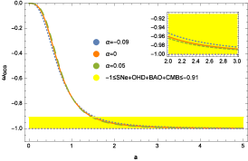
Figure 1: Equation of state parameter of GCG DE versus scale factor $a$, considering $\Omega_{GCG}=0.956$ and $\alpha=-0.09$ 46 , $\alpha=0$ and $\alpha=0.05$ 461 .

$$\dot{\rho}_{\Lambda}=-\frac{3DH}{a^{3\beta}}\left(K+Da^{-3\beta}\right)^{-\frac{\alpha}{\beta}}.$$ (21)

Using Eqs. (19) and (20), the EoS parameter of the GCG model of DE is obtained as

$$\omega_{\Lambda}=-1+\frac{Da^{-3\beta}}{K+Da^{-3\beta}}.$$ (22)

$\omega_{\Lambda 0}=-K/(K+D)$ is the present value of the EoS parameter. In the following, we consider the cosmology model with values of parameters: $\Omega_{GCG}=0.956$ and $\alpha=-0.09$ 46 , $\alpha=0$, which can be reduced to the standard DE plus DM models and $\alpha=0.05$ 461 . We have plotted the evolution of the EoS parameter of GCG DE with respect to the scale factor $a$ in Fig. (1). We see that the EoS parameter translates the universe from matter region towards vacuum DE region. The curves representing the GCG are very similar, only the initial slope changes with the change of the $\alpha$ parameter. Ref. 46 found that the best fit evolution of $\omega_{GCG}$ is $-1\leq\omega_{GCG}\leq-0.91$ and this result is consistent with 47 . Now introduce the squared speed of GCG fluid as

$$v_{s}^{2}=\frac{p^{\prime}_{\Lambda}}{\rho^{\prime}_{\Lambda}}=\omega^{\prime}_{\Lambda}\frac{\rho_{\Lambda}}{\rho^{\prime}_{\Lambda}}+\omega_{\Lambda},$$ (23)

which now becomes

$$v_{s}^{2}=\frac{K\alpha a^{-3(1+\alpha)}}{D+K\alpha a^{-3(1+\alpha)}}.$$ (24)

It is found that the model admits a positive squared speed for $\alpha>0$. Thus for a stable model we require $\alpha$ positive.
In the following, we regard the scalar field model as an effective description of an underlying theory of DE with energy density and pressure

$$\rho_{\phi} = 1/2\dot{\phi^{2}}+V(\phi)=\left(K+Da^{-3\beta}\right)^{\frac{1}{\beta}},$$ (25)

$$p_{\phi} = 1/2\dot{\phi^{2}}-V(\phi)=-K\left(K+Da^{-3\beta}\right)^{-\frac{\alpha}{\beta}},$$ (26)

where $\dot{\phi}^{2}$ and $V(\phi)$ are termed as kinetic energy and scalar potential, respectively. Now by using Eqs. (25) and (26) we can easily obtain the potential and the kinetic energy terms as

$$\dot{\phi^{2}} = \frac{Da^{-3\beta}}{\left(K+Da^{-3\beta}\right)^{\frac{\alpha}{\beta}}},$$ (27)

$$V(\phi) = \frac{K+\frac{D}{2}a^{-3\beta}}{\left(K+Da^{-3\beta}\right)^{\frac{\alpha}{\beta}}}.$$ (28)

The above equation shows that $\dot{\phi^{2}}<0$ (giving negative kinetic energy) for $Da^{-3\beta}<0$. Therefor one can concludes that the scalar field $\phi$ is a phantom field. Efstathiou et al. 48 provided the simplest quintessence models and obtained the range of value $\omega_{q}$ is $\omega_{q}\leq-0.6$. To keep thing the simple model, then, we shall use a potential $V\propto q^{-2}$. As a reference, it is relevant to mention that long back, Hoyle and Narlikar used C-field (a scalar called creation) with negative kinetic energy for steady state theory of the universe 49 . In the next sections we consider the above equations to determine the potential in the two cases (i) holographic DE (ii) new agegraphic DE.

III Correspondence between the interacting holographic DE and generalized Chaplygin gas model in anisotropy universe

In this section we consider a non-isotropic universe. Here our choice for holographic DE density is 17

$$\rho_{\Lambda}=\frac{3c^{2}}{R_{h}^{2}},$$ (29)

$R_{h}$ is the future event horizon. Suggestive as they are, these ideas provide no indication about how to pick out the IR cutoff in a cosmological context. We are interested in the one proposed in 18 :

$$R_{h}=a\int^{\infty}_{t}\frac{dt}{a}=a\int^{\infty}_{x}\frac{dx}{aH},$$ (30)

where $x=\ln a$. Note that the presence of a vacuum energy component makes the above integration confined. In the case of non-interacting fluid the conservation equation for DM can be written as

$$\rho_{m}=\rho_{m0}a^{-3(1+\omega_{m})}=\rho_{m0}(1+z)^{3(1+\omega_{m})}.$$ (31)

We recalls that the reconstruction method is limited to pressureless fluids, so Eq. (31) reduces to $\rho_{m}\propto(1+z)^{3}$ when dust matter $\omega_{m}=0$ is assumed. In 18 , a convenient method to solve equations is carried out by taking $\Omega_{\Lambda}=\rho_{\Lambda}/\rho_{cr}=c^{2}/R_{h}^{2}H^{2}$ as the unknown function. The time derivative of the future horizon is given by:

$$\dot{R}_{h}=R_{h}H-1=\frac{c}{\sqrt{\Omega_{\Lambda}}}-1.$$ (32)

Taking the derivative with respect to the cosmic time of (29) and using (32) we get

$$\dot{\rho}_{\Lambda}=2H\left(\frac{\sqrt{\Omega_{\Lambda}}}{c}-1\right)\rho_{\Lambda}.$$ (33)

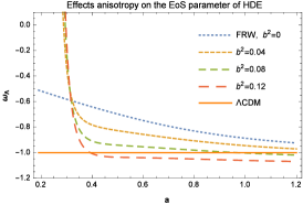
Figure 2: Evolutions of $\omega_{\Lambda}$ with and without interaction. The rest of parameter are $c=1$ and $\Omega_{\sigma 0}=0.001$.

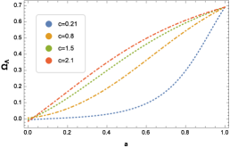
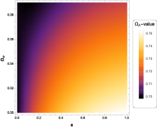
Figure 3: The first figure representations of $\Omega_{\Lambda}$ for different $c$ and $\Omega_{\sigma 0}=0.001$ while second figure representations of $\Omega_{\Lambda}$ versus $\Omega_{\sigma}$ and $a$ for $c=1$. We take for both $b^{2}=0.02$.

Substituting Eqs. (18), (29) and (33) into (16) and using definition $r=(1-\Omega_{\sigma}-\Omega_{\Lambda})/\Omega_{\Lambda}$, gives the EoS parameter of the interacting HDE model as

$$\omega_{\Lambda}=-\frac{1}{3}-\frac{2\sqrt{\Omega_{\Lambda}}}{3c}-\frac{b^{2}}{\Omega_{\Lambda}}(1-\Omega_{\sigma}).$$ (34)

In the far future $(a\rightarrow\infty$, $\Omega_{\sigma}\rightarrow 0$ and $\Omega_{\Lambda}\rightarrow 1)$, one has $\omega_{\Lambda}=-1/3-2/3c$, so the HDE model does not involve the $\Lambda$CDM model. In the absence of interaction between HDE and CDM, $b^{2}=0$, using Eq. (34), one can see that by considering $c\leq\sqrt{\Omega_{\Lambda}}$. We test this scenario for the interaction between HDE and DM by using some observational results. For the comparison with the phenomenological interacting model, in our scenario the coupling between HDE and DM can be expressed as a counterpart of $b^{2}$ as in the phenomenological interaction form. In fact, $b^{2}$ is within the region of the golden supernova data fitting result $b^{2}=0.00^{+0.11}_{-0.00}$ 50 and the observed CMB low $l$ data constraint 51 . Now we use 73 SGL data points to estimate $c$ in the model of Markov-Chain Monte Carlo package CosmoMC is $c=1.9730^{+0.0270}_{-0.8993}$ 511 , the another best-fit from the strong gravitational lensing (SGL) data is $c=0.8335^{+0.8031}_{-0.3495}$, with CBS (CMB+BAO+SN) it is $c=0.6458^{+0.0472}_{-0.0483}$, the SGL+CBS data is $c=0.6429^{+0.0515}_{-0.0436}$, and the $w$CDM model, with the SGL+CBS is $\Omega_{m0}=0.2891^{+0.0100}_{-0.0092}$ and $w=-1.0546^{+0.0606}_{-0.0610}$ 512 .
In the numerical calculations, we set $c=1$ and $\Omega_{\Lambda}^{0}=0.69$. Figure (2) shows that for $b^{2}=0$, $\omega_{\Lambda}$ decreases from $-0.34$ at early times while for $b^{2}\neq 0$ it can be observed that the EoS parameter starts from matter dominant and goes towards lower negative value of phantom region for all of the cases of interacting parameter. This behavior arises the shear scalar evolves as $\sigma^{2}\propto a^{-6}$. Moreover it show that for $b^{2}>0.04$, $\omega_{\Lambda}\sim-1.06$ at present times i.e. $a\rightarrow 1$. This is recorder with the observations 52 . Another best fit data with the holographic model is $c=0.21$ 521 with SNe Ia, $c=0.7$ 522 with BOOMERANG and WMAP data on the CMB and $c=2.1$ 523 with small $l$ CMB data. In particular, we have schemed the evolution of $\Omega_{\Lambda}$ versus scale factor $a$ in an anisotropic universe as shown in figure. (3). In left panel of Fig. (3), for a given $c$, it is to find that, $\Omega_{\Lambda}$ increases simultaneity when the $a$ increases; for a given $a$, $\Omega_{\Lambda}$ increases when the $c$ increases. Finally, figure (3) (right panel) show the effects of the anisotropic on the evolutionary behaviour the holographic Chaplygin gas DE model.
The main purpose of this work is to investigate correspondence between the Chaplygin gas DE model and the holographic DE model in the flat anisotropy universe case. Using Eqs. (20), (22), (29), (32) and (34), we determine the parameters as

$$K=(3H^{2}\Omega_{\Lambda})^{\beta}-Da^{-3\beta},$$ (35)

$$D=(3H^{2}\Omega_{\Lambda}a^{3})^{\beta}\left(\frac{2}{3}-\frac{2}{3}\frac{\sqrt{\Omega_{\Lambda}}}{c}-\frac{b^{2}}{\Omega_{\Lambda}}(1-\Omega_{\sigma})\right).$$ (36)

Substituting Eq. (36) into (35) reduces to

$$K=(3H^{2}\Omega_{\Lambda})^{\beta}\left(\frac{1}{3}+\frac{2}{3}\frac{\sqrt{\Omega_{\Lambda}}}{c}+\frac{b^{2}}{\Omega_{\Lambda}}(1-\Omega_{\sigma})\right).$$ (37)

Now we can rewritten the scalar potential and kinetic energy term as following

$$\dot{\phi^{2}} = 2H^{2}\left(\Omega_{\Lambda}-\frac{\Omega^{\frac{3}{2}}_{\Lambda}}{c}-\frac{3b^{2}}{2}(1-\Omega_{\sigma})\right),$$ (38)

$$V(\phi) = H^{2}\left(2\Omega_{\Lambda}+\frac{\Omega^{\frac{3}{2}}_{\Lambda}}{c}+\frac{3b^{2}}{2}(1-\Omega_{\sigma})\right).$$ (39)

We now substitute $x=\ln a$, to alter the time derivative into the derivative with logarithm of the scale factor, which is the most useful function in this case. Consequently from definition $\dot{\phi}=H\phi^{\prime}$, one can rewrite Eq. (38) as

$$\phi^{\prime}=\sqrt{2}\left(\Omega_{\Lambda}-\frac{\Omega^{\frac{3}{2}}_{\Lambda}}{c}-\frac{3b^{2}}{2}(1-\Omega_{\sigma})\right)^{\frac{1}{2}},$$ (40)

where the prime denotes the differentiation with respect to the time parameter $x$, Eq. (40) becomes

$$\phi(a)-\phi(a_{0})=\int_{0}^{a}\frac{1}{a}\sqrt{2\left(\Omega_{\Lambda}-\frac{\Omega^{\frac{3}{2}}_{\Lambda}}{c}-\frac{3b^{2}}{2}(1-\Omega_{\sigma})\right)}da,$$ (41)

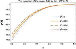
Figure 4: The evolutionary scalar field $\phi$ for the interacting HDE and GCG with different $b^{2}$. Auxiliary parameters are $\Omega^{0}_{\Lambda}=0.69$, $\phi(1)=0$, $H_{0}=72$, $c=1$ and $\Omega_{\sigma 0}=0.001$.

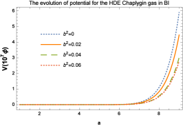
Figure 5: The reconstruction of the potential for the interacting HDE and GCG with different $b^{2}$. Auxiliary parameters as in Fig. (4).

where we take a $a_{0}=1$ for the present time, the evolution $\Omega_{\Lambda}$ and $H$ is given by HDE in BI universe . The evolutionary form of the scaler field and the reconstructed potential $V(\phi)$ are plotted in Figs. (4) and (5), where again we have taken $\phi(a_{0}=1)=0$ for the present time. Again, figure (4) shows that $\phi(a)$ goes up as the scale factor increases here the stronger interaction is, the slower $\phi(a)$ which changes as the scale factor increases. Figure (5) illustrate that $V(\phi)$ could increase with the increasing $a$, i.e. the stronger the interaction is, the slower the $V(\phi)$ varies. Furthermore, $V(\phi)$ for the HDE and GCG without interaction increase faster than that with interaction. To complete, the effective EoS parameter an anisotropic universe is obtain as

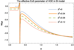
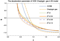
Figure 6: The evolutions of $\omega_{eff}$ and $q$ with scale factor for the interacting HDE with $\Omega^{0}_{\Lambda}=0.69$, $c=1$ and $\Omega_{\sigma 0}=0.001$, GCG model with $A_{s}=0.7$ and $\alpha=0.02$ and $\Lambda$CDM model with $\Omega_{m0}=0.3$ and $\Omega^{0}_{\Lambda}=0.7$.

$$\omega_{eff}=\frac{p_{\Lambda}}{\rho_{m}+\rho_{\Lambda}}=\frac{\Omega_{\Lambda}}{1-\Omega_{\sigma}}\left(\frac{\frac{1}{2}\dot{\phi}^{2}-V(\phi)}{\frac{1}{2}\dot{\phi}^{2}+V(\phi)}\right).$$ (42)

Inserting Eqs. (38) and (39) into (42), we obtain

$$\omega_{eff}=-\frac{\Omega_{\Lambda}+\frac{2}{c}\Omega_{\Lambda}^{\frac{3}{2}}+3b^{2}(1-\Omega_{\sigma})}{3(1-\Omega_{\sigma})}.$$ (43)

With the help Eqs. (15), (25), (26), (36) and (37), we give the deceleration parameter in BI universe

$$q=\frac{1}{2}(1-\Omega_{\Lambda})+\frac{3}{2}\Omega_{\sigma}-\frac{\Omega^{\frac{3}{2}}_{\Lambda}}{c}-\frac{3b^{2}}{2}(1-\Omega_{\sigma}).$$ (44)

If we take $\Omega_{\Lambda 0}=0.69$, $c=1$ and $\Omega_{\sigma 0}=0.001$ for now i.e., $a=1$, then Eq. (43) gives $\omega_{eff}<-1$ when $b^{2}>0.08$. We plot in Fig. (6) the evolutions of the $\omega_{eff}$ and $q$ of the interacting HDE and GCG with different $b^{2}$. From left panel of Fig. 6 we see that the $\omega_{eff}$ of the interacting HDE and GCG cannot cross the phantom divide at present times. Right panel of Fig. 6 presents that the universe transitions from a matter dominated epoch at early times to the acceleration phase in the future, as expected. We find that the behaviour of the deceleration parameter for the best-fit universe is quite different from that in the GCG model and $\Lambda$CDM cosmology. In addition, for the case of interacting HDE, we have a cosmic deceleration to acceleration phase at range of $0.48\leq a\leq 0.66$ which is matchable with the observations 53 . For case of $b^{2}=1.2$, the present value of the best-fit deceleration parameter, $q_{0}=-0.6$, is significantly smaller than $q_{0}=-0.55$ for the $\Lambda$CDM model with $\Omega_{m0}=0.3$ and also larger than $q_{0}=-0.73$ 54 .
Now, we analyze the model which is using the observational tests: the differential age of old objects based on the $H(z)$ dependence as well as the data from SGL+CBS and $w$CDM. The redshift-drift observation, that is called the “SL test”, is not the only conceptually simple, but also is a direct probe of cosmic dynamic expansion, although being observationally challenging. In Ref. 541 introduced the redshift relation by the a spectroscopic velocity shift $\triangle\nu$ as $\triangle\nu\equiv\triangle z/(1+z)$. By using the Hubble parameter $H(z)=-\dot{z}/(1+z)$, we obtain 542

$$\triangle\nu=H_{0}\triangle t_{0}\bigg{(}1-\frac{\widetilde{H}}{1+z}\bigg{)},$$ (45)

where $\widetilde{H}=H/H_{0}$ and we have normalized the scale factor to $a(t_{0})=1$ and neglected the contribution from relativistic components. The parameter $\widetilde{H}(z)$ contains all the details of the cosmological model under investigation. It is clear that the function $\widetilde{H}(z)$ is related to the spectroscopic velocity shift via Eq. (45). We will examine the Sandage-Loeb (SL) test, and then examine effects of anisotropy on the HDE and GCG models in the SL test. In figure (7) we plot $\triangle\nu$ as function of the source redshift in the flat BI model case for different values of $\Omega_{\sigma 0}$ assuming a time interval $\triangle t_{0}=10$ years for this models. From Fig. (7) we see that the interacting holographic and generalized chaplygin gas DE can be distinguished from the SGL+CBS and the $w$CDM models via the SL test. In other words, the models shown in Fig. (7) can be easily discriminated using current cosmological tests of the background expansion. Also we can see that for the case of $\Omega_{\sigma 0}=0.02$, $\triangle\nu$ is positive at small redshifts and becomes negative at $z>0.64$, while for $\Omega_{\sigma 0}\neq 0.02$, $\triangle\nu$ is negative in all range of redshift. Besides, the amplitude and slope of the signal depend mainly on $\Omega_{\sigma 0}$.

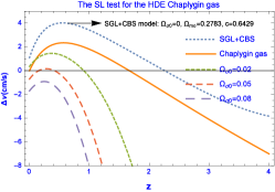
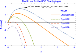
Figure 7: The SL test for the HDE Chaplygin gas model for different value of $\Omega_{\sigma 0}$ by comparing with models as the SGL+CBS model (left panel) and $w$CDM model (right panel). We take for the case of HDE with $\Omega_{m0}=0.28$, $c=1$, $b^{2}=0.02$ and $H_{0}=72~{}kms^{-1}Mpc^{-1}$ 543 and GCG model with $A_{s}=0.7$ and $\alpha=0.02$.

IV Correspondence between the interacting new agegraphic DE and Chaplygin gas model of DE in anisotropy universe

In this section, we first review the NADE model. The energy density of the NADE can be written 27

$$\rho_{\Lambda}=\frac{3n^{2}}{\eta^{2}},$$ (46)

where the conformal time is given by

$$\eta=\int\frac{dt}{a(t)}=\int\frac{da}{Ha^{2}}.$$ (47)

If we write $\eta$ to be a definite integral, there will be an integral constant in addition. Thus, we have $\dot{\eta}=1/a$. Now, the fractional energy density of the NADE is given by

$$\Omega_{\Lambda}=\frac{n^{2}}{H^{2}\eta^{2}}.$$ (48)

Taking the derivative of Eq. (46) with respect to the cosmic time and using (48) we get

$$\dot{\rho}_{\Lambda}=-2H\frac{\sqrt{\Omega_{\Lambda}}}{na}\rho_{\Lambda}.$$ (49)

Inserting Eq. (49) into the continuity equation (16), we obtain the EoS parameter of NADE

$$\omega_{\Lambda}=-1+\frac{2\sqrt{\Omega_{\Lambda}}}{3na}-\frac{b^{2}}{\Omega_{\Lambda}}(1-\Omega_{\sigma}).$$ (50)

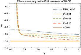
Figure 8: Evolutions of $\omega_{\Lambda}$ of NADE with and without interaction. The rest of parameters are $\Omega_{\Lambda}^{0}=0.69$, $n=2.7$ and $\Omega_{\sigma 0}=0.001$.

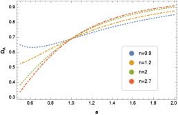
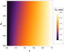
Figure 9: Left panel representations of $\Omega_{\Lambda}$ for the NADE with $a$ for various model parameters $n$ and $\Omega_{\sigma 0}=0.001$ while right panel representations of $\Omega_{\Lambda}$ versus $a$ and $\Omega_{\sigma}$ for $n=2.7$. For both cases, we take $b^{2}=0.02$.

It is important to note that when $b^{2}=0$, the interacting DE becomes inevitable and Eq. (50) reduces to its respective expression in new ADE in general relativity 55 . In the case of ($b^{2}=0$), the present accelerated expansion of our universe can be derived only if $n>1$ 27 . Note that we take $a=1$ for the present time. In addition, $\omega_{\Lambda}$ is always larger than $-1$ and cannot cross the phantom divide $\omega_{\Lambda}=-1$. However, in the presence of the interaction, $b^{2}\neq 0$, taking $\Omega_{\Lambda 0}=0.69$, $\Omega_{\sigma}=0.001$, $n=2.7$ 28 and $a=1$ for the present time, Eq. (50) gives

$$\omega_{\Lambda}=-0.795-1.45b^{2}.$$ (51)

It is clear that the phantom EoS $\omega_{\Lambda}<-1$ can be obtained when $b^{2}>0.14$ for the coupling between NADE and CDM. In the late time where $\Omega_{\Lambda}\rightarrow 1$, $\Omega_{\sigma}\rightarrow 0$ and $a\rightarrow\infty$ we have $\omega_{\Lambda}=-1-b^{2}$. Thus $\omega_{\Lambda}<-1$ for $b^{2}>0$. This implies that in the late time $\omega_{\Lambda}$ necessary crosses the phantom divide in the presence interacting DM and DE. In the numerical calculations, we set $n=2.7$, $\Omega_{\Lambda}^{0}=0.69$ and $\Omega_{\sigma 0}=0.001$. From Fig. (8) we see that for $b^{2}\neq 0$, $\omega_{\Lambda}$ decreases from matter dominant at early times while for $b^{2}=0$ (FRW), $\omega_{\Lambda}$ decreases with the $a$ increase and its less steep compared to an interaction term at late times. We see that for $b^{2}=1.2$, $\omega_{\Lambda 0}=-0.96$ at present time. Therefore the EoS parameter is consistent with the WMAP observation 551 . In figure (9) (left panel), we plot the evolution of the density parameter $\Omega_{\Lambda}$ for $b^{2}=0.02$ as a function of the $a$ for different value of $n$. Moreover, we can see that at the early time $\Omega_{\Lambda}$ decreases with the increase of $n$, while increases with the increase of $n$ when $a>0$. Also the anisotropy effects are clearly seen in right panel of figure (9). So the $\Omega_{\Lambda}$ decreases slowly with increasing of $\Omega_{\sigma}$. This is consistent with Eq. (14).
Next, we suggest a correspondence between the new agegraphic DE scenario and the generalized Chaplygin gas DE model. To do this, comparing Eqs. (50), (22) and using (35), we reach

$$K=(3H^{2}\Omega_{\Lambda})^{\beta}\left(1-\frac{2\sqrt{\Omega_{\Lambda}}}{3na}+\frac{b^{2}}{\Omega_{\Lambda}}(1-\Omega_{\sigma})\right),$$ (52)

and

$$D=(3H^{2}\Omega_{\Lambda}a^{3})^{\beta}\left(\frac{2\sqrt{\Omega_{\Lambda}}}{3na}-\frac{b^{2}}{\Omega_{\Lambda}}(1-\Omega_{\sigma})\right).$$ (53)

We reconstruct the kinetic energy and scalar potential term as

$$\dot{\phi^{2}} = H^{2}\left(-3b^{2}(1-\Omega_{\sigma})+\frac{2\Omega^{\frac{3}{2}}_{\Lambda}}{na}\right),$$ (54)

$$V(\phi) = H^{2}\left(3\Omega_{\Lambda}+\frac{3b^{2}}{2}(1-\Omega_{\sigma})-\frac{\Omega^{\frac{3}{2}}_{\Lambda}}{na}\right).$$ (55)

Now since definition $\dot{\phi}=H\phi^{\prime}$, we get

$$\phi(a)-\phi(a_{0})=\int_{0}^{a}\frac{1}{a}\sqrt{-3b^{2}(1-\Omega_{\sigma})+\frac{2\Omega^{\frac{3}{2}}_{\Lambda}}{na}}da,$$ (56)

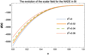
Figure 10: The evolutionary scalar field $\phi$ for the interacting NADE and GCG with different $b^{2}$ considering $\Omega_{\Lambda}^{0}=0.69$, $\Omega_{\sigma 0}=0.001$, $n=2.7$ and $\phi(1)=0$.

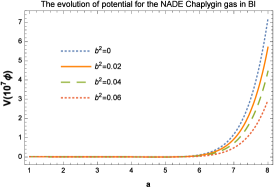
Figure 11: The reconstruction of the potential for the interacting NADE and GCG with different $b^{2}$. Auxiliary parameters as in Fig. (10).

where $a_{0}$ is the present time value of the scale factor, $\Omega_{\Lambda}$ and $H$ is given by NADE in BI universe . Therefore, we have established an interacting new agegraphic and generalized Chaplygin gas DE model and reconstructed the potential and the dynamics of scalar field in an anisotropic universe. The evolution of the scalar filed, Eq. (56), for three different values of $b^{2}$ is plotted in Fig. (10). Figure (10) shows that the scalar field increases (and hence the kinetic energy $\dot{\phi}^{2}$ of the potential increases) with the passage of time. The potential $V(\phi)$ versus $a$ for three different value of the $b^{2}$ are shown in figure (11), indicating the increasing behavior. Also, we can see that at the initial time there is no difference between various values of $b^{2}$. After that, increasing $b^{2}$ decreases the value of $V(\phi)$.
Inserting Eqs. (54) and (55) into (42), we obtain the effective EoS parameter an anisotropic universe

$$\omega_{eff}=-\frac{\Omega_{\Lambda}}{1-\Omega_{\sigma}}+\frac{2}{3na}(\frac{\Omega^{\frac{3}{2}}_{\Lambda}}{1-\Omega_{\sigma}})-b^{2}.$$ (57)

Finally, we give the deceleration parameter of interacting NADE and GCG in BI universe

$$q=\frac{1}{2}(1-3\Omega_{\Lambda})+\frac{3}{2}\Omega_{\sigma}+\frac{\Omega^{\frac{3}{2}}_{\Lambda}}{na}-\frac{3}{2}b^{2}(1-\Omega_{\sigma}).$$ (58)

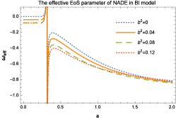
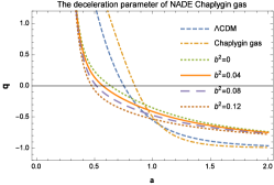
Figure 12: The evolutions of $\omega_{eff}$ and $q$ with scale factor for the interacting NADE with $\Omega^{0}_{\Lambda}=0.69$, $n=2.7$ and $\Omega_{\sigma 0}=0.001$, GCG model with $A_{s}=0.7$ and $\alpha=0.02$ and $\Lambda$CDM model with $\Omega_{m0}=0.3$ and $\Omega^{0}_{\Lambda}=0.7$.

If we take $\Omega_{\Lambda 0}=0.69$, $\Omega_{\sigma}=0.001$, $n=2.7$ 28 and $a=1$ for the present time, then Eq. (57) will give $\omega_{eff}<-1$ when $b^{2}>0.45$. This mentions that the EoS parameter has a phantom behavior. The evolution of the effective EoS and deceleration parameter is plotted in Fig. (12). From left panel of Fig. (12) we see that for all of the cases of interacting parameter, $\omega_{eff}$ of the NADE cannot have a transition from $\omega_{eff}<-1$. Recent studies have constructed $q(z)$ takeing into account that the strongest evidence of accelerations happens at redshift of $z\sim 0.2$. In order to do so, the researcher have set $q(z)=1/2(q_{1}z+q_{2})/(1+z)^{2}$ to reconstruct it and after that they have obtained $q(z)\sim-0.31$ by fitting this model to the observational data 56 ; 57 . Also it found that $q<0$ for $0\leqslant z\leqslant 0.2$ within the $3\sigma$ level. Under such circumstances and considering the Eq. (58), the present value of the deceleration parameter for the interacting NADE in BI models with $b^{2}=0.12$ is $q_{0}\sim-0.53$ which is consistent with observations 58 . Moreover, for the case of interacting NADE, transition from deceleration to acceleration occurs at rang of $0.47\leq a\leq 0.63$. For the flat $\Lambda$CDM model, the deceleration parameter $q$ passes the transition point at $a=0.56$ 581 . Eventually, the universe will undergo accelerated expansion at the late time forever and cannot come back to decelerated expansion, as shown in Fig. (12). These behaviors are similar Refs. 27 ; 28 . In addition to, the fall of $q$ with scale factor is much steeper in the case GCG and $\Lambda$CDM models in compare with interacting NADE model.
Finally, we examine the Sandage-Loeb (SL) test, and then examine effects of anisotropy on the NADE Chaplygin gas in the SL test. To do this using Eq. (45) we can obtain

$$\triangle\nu=H_{0}\triangle t_{0}\bigg{(}1-(1+z)^{-1}(\frac{\Omega_{m0}(1+z)^{3}+\Omega_{\sigma 0}(1+z)^{6}}{1-\Omega_{\Lambda}})^{\frac{1}{2}}\bigg{)},$$ (59)

where we set $\triangle t_{0}=10$ years and $\Omega_{\Lambda}$ is given by (48). We reconstruct the velocity shift behavior in the NADE Chaplygin gas model respect $z$ for different value of the $\Omega_{\sigma 0}$ in Fig . (13). We have chosen the fractional matter density $\Omega_{m0}=0.274$ from $\Lambda$CDM 59 and $n=2.807$ 60 . From Fig. (13) we see that the new agegraphic and generalized Chaplygin gas DE in BI model can be distinguished from the $\Lambda$CDM model via the SL test.

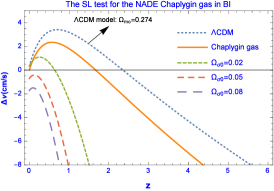
Figure 13: The SL test for the NADE Chaplygin gas model for different value of the anisotropy energy density parameter $\Omega_{\sigma 0}$ and the $\Lambda$CDM model. We take $\Omega_{m0}=0.28$, $b^{2}=0.02$ and $n=2.8$.

V Cosmological evolution of the Hubble parameter of different dark energy in BI universe and comparison with the $\Lambda$CDM model

In the section, we further compare the expansion rate $H(z)$ with that predicted by different models i.e., HDE, NADE, GCG and $\Lambda$CDM. As recently proposed by 61 , these can be used to determine $H(z)=-\frac{1}{1+z}\frac{dz}{z}$. Therefore a determination of $dz/dt$ directly measures $H(z)$. In 61 it was demonstrated the feasibility of the method by applying it to a $z\sim 0$ sample. For the comparison with the phenomenological interacting model, in our scenario the coupling between HDE, NADE, GCG and DM can be expressed by $b^{2}$ parameter as in the phenomenological interaction form. The constraint results from CMB and BAO presented that the mean values of interaction rate were $b^{2}=-0.61^{+0.12}_{-0.25}$ from CMB and BAO measurements 62 , $b^{2}=-0.67^{+0.086}_{-0.17}$ from CMB and Hubble Space Telescope (HST) tests 63 , and $b^{2}=0.00328^{+0.000736+0.00549+0.00816}_{-0.00328-0.00328-0.00328}$ from the redshift space distortion (RSD) date 64 . Fig. (14) shows the comparison of the $H(z)$ estimates with different cosmological models for the cases of $H_{0}=72~{}kms^{-1}Mpc^{-1}$, $\Omega_{\sigma 0}=0.001$ and $b^{2}=0.02$ with an anisotropic universe. The values of $H(z)$ are fully compatible with $\Lambda$CDM, constraining the expansion rate very firmly. The redshift range $0.5<z<2$ is critical to disentangle many different cosmologies, as can be seen from Fig. (14). It is shown that in a BI model although HDE model performs a little poorer than $\Lambda$CDM model, but it performs better than NADE and GCG models. So, among these three DE models, HDE in BI is more favored by the observational data. Again we plot the $H(z)$ and effects of anisotropy on both the HDE and NADE as shown in figure (15). From Fig. (15), we can clearly see that for different $\Omega_{\sigma 0}$ parameter value the process of cosmic evolution looks quite similar, i.e., the bigger value the $\Omega_{\sigma 0}$ parameter is taken, the best value the Hubble expansion rate $H(z)$ is gotten. This implies that the BI model would play a more important role for constraining the models with more parameters.

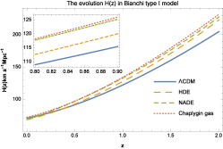
Figure 14: The value of the Hubble parameter as a function of redshift as derived from the four models with $\Omega_{\sigma 0}=0.001$ $c=0.818$, $n=2.807$, $A_{s}=0.7$, $\alpha=0.02$, $\Omega_{m0}=0.277$ 60 and $H_{0}=72~{}kms^{-1}Mpc^{-1}$ 543 .

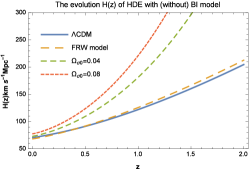
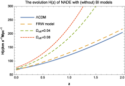
Figure 15: The evolution of $H(z)$ versus redshift $z$ of both the HDE and NADE for different values of parameter $\Omega_{\sigma 0}$. The rest of parameters are the same as for Fig. (14).

VI Linear perturbation theory in anisotropic universe

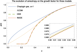
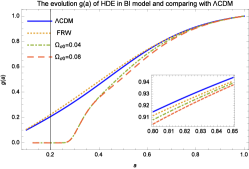
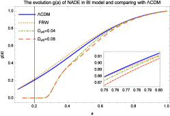
Figure 16: Right panel: Time evolution of the growth factor as a function of the scale factor for the three cosmological models in an anisotropic universe. To compare the three models, we thus fix the variance for the HDE and NADE model ($\Omega_{\sigma 0}=0.001$). Middle panel: Time evolution of the growth factor for different value of the anisotropy energy density parameter $\Omega_{\sigma 0}$ and comparing to the $\Lambda$CDM and FRW in HDE models with $c=1$. Left panel: Same as middle panel for NADE with $n=2.7$.

Finally, we discuss the linear perturbation theory of non-relativistic dust matter, $g(a)$, for the different DE models and compare it with the solution found for the $\Lambda$CDM and FRW models. The differential equation for the evolution of the growth factor $g(a)$ is given by 66 ; 67

$$g^{\prime\prime}(a)+(\frac{3}{a}+\frac{E^{\prime}(a)}{E(a)})g^{\prime}(a)-\frac{3}{2}\frac{\Omega_{m0}}{a^{5}E^{2}(a)}g(a)=0,$$ (60)

where $E=H/H_{0}$. For a non interacting DE model, we solve numerically Eq. (60) for studying the linear growth with four DE models in BI. Then, we compare the linear growth in the HDE and NADE generalized Chaplygin gas models with the linear growths in the $\Lambda$CDM and FRW models. To evaluate the initial conditions, since we are in the linear regime, we take that the linear growth factor has a power law solution, $g(a)\propto a^{n}$, with $n>1$, then the linear growth should grow in time. In Fig. (16) we show the growth factor by the scale factor $a$ for the three DE models considered in this work, as compared to the $\Lambda$CDM and FRW models. The left panel show that the growth factor in the GCG model is larger than the three DE models seen in this work. But for small scale factors, the growth factor in the $\Lambda$CDM model is larger than those of HDE and NADE models, while for the range of $0.49<a<0.73$, it becomes smaller than those of HDE and NADE models, then it is again greater than the that of HDE and NADE models. This means that, at the beginning, the growth factor in anisotropy for DE models is zero and the $\Lambda$CDM is more efficient than HDE and NADE models. In both the middle and right figure (16), we see that in the FRW model, the growth factor evolves proportionally to the scale factor, as expected. For the $\Lambda$CDM model, we notice that the evolution of $g(a)$ evolves more slowly than in the FRW case. In the cases of HDE and NADE models with $\Omega_{\sigma 0}\neq 0$ (anisotropic universe), $g(a)$ is smaller even when compared to the $\Lambda$CDM model. However, for rather larger scale factors, the growth factor in the FRW universe becomes smaller than the $\Lambda$CDM model while it is still larger enough than that of HDE and NADE models in an anisotropic universe. This result is consistent with Ref. 68 .

VII Conclusion

We have considered a correspondence between the interaction of HDE and NADE scenarios and the Chaplygin gas model of DE in an anisotropic universe. In particular, we reconstructed the field equations of DE model in an anisotropic universe. The Chaplygin gas model plays a very crucial role in the EoS fluid description of DE in cosmology. The constraints on the GCG model are given by using observations of SNe+OHD+BAO+CMB 46 ; 461 ; 47 . The only parameter in this model which needs to be fitted by observational data is the parameter $\alpha=-0.09,0,0.05$. Furthermore, it is shown that the GCG model in BI can drive the universe from a matter dominated phase to an accelerated expansion phase, behaving like matter in early times and as vacuum DE region i.e., $\omega_{GCG}\rightarrow-1$ at late times, which it consistent with the observational data 46 ; 461 ; 47 . Then we have described this “GCG” as BI universe having a scalar field and found its self-interacting potential. In what follows, we have presented the evolution of GCG models for both the HDE and NADE depending on the values of parameters. For the case of HDE dominated universe, i.e., $\Omega_{\Lambda}\sim 1$; if we consider $c>1$ and $b^{2}=0$ (non interaction) then the expansion will in quintessence regime, while for $c<1$, phantom evolution of the universe can be observed. Besides, it can be observed that for selected value $b^{2}>0.04$, the EoS parameter can cross the phantom region and $\omega_{\Lambda}\sim-1.06$ at present times which the model has agreement with Ref. 52 (see Fig. (2)). But in case of NADE having $\Omega_{\Lambda}\sim 1$, shows that EoS parameter can be less than $-1$ if $b^{2}=0$ and $n<0$ but observational points of view propose $n=2.76^{+0.11130}_{-0.109}$ 27 ; 28 which permits the phantom era. We also reconstructed the dynamics and the potential of the Chaplygin gas scalar field according the evolution of both the interacting HDE and NADE models which can describe the phantomic accelerated expansion of the BI universe. To do that the holographic and new agegraphic Chaplygin gas scalar field for a given $b^{2}$ increases with increasing the scale factor. Also for a given scale factor, it increases with increasing $b^{2}$. The holographic and new agegraphic Chaplygin potential $V(\phi)$ for a given $b^{2}$, increases with increasing the scalar filed. For a given scalar field, $V(\phi)$ decreases with increasing $b^{2}$. These results have been shown in figures (4), (5), (10) and (11). On the basis of the above considerations, it seems reasonable to investigate an anisotropic universe, in which the present cosmic acceleration is followed by a decelerated expansion in an early matter dominant phase. In other words, it indicates that the values of transition scale factor and current deceleration parameter are $a\sim 0.84$ and $q_{0}=-0.49$ for the case of generalized Chaplygin gas, $0.48\leq a\leq 0.66$ and $q_{0}=-0.6$ for the case of holographic DE with $b^{2}=1.2$ and $0.47\leq a\leq 0.63$, $q_{0}=-0.53$ for new agegraphic DE model while for the case of $\Lambda$CDM model, the deceleration parameter passes the transition point at $a=0.56$ 581 . This description is allows for an unambiguous confrontation with observational data. For this purpose, several studies were performed aiming to constrain the parameter space of the model using observations data. In particular, the holographic and new agegraphic DE and GCG models was explored with the SL test in BI model. In order words, the best way to probe models with such interaction between DM and DE is to map out cosmic expansion during the matter dominated phase. The SL tests offers a unique tool to do just that. So, the SL test can be used to distinguish the HDE, NADE and GCG in BI model from the $\Lambda$CDM, the $w$CDM and the SGL+CBS models and it was observed that the constraint on $\Omega_{\sigma 0}$ is very strong (see Figs. (7) and (13)). For the case of $\Omega_{\sigma 0}=0.02$, $\triangle\nu$ was positive at small redshifts and negative at $z>0.64$, while for $\Omega_{\sigma 0}\neq 0.02$, $\triangle\nu$ was negative in all range of redshift. We have used the Hubble parameter versus redshift data to constrain cosmological parameters of HDE and NADE of GCG models in BI universe. The constraints are consistent with observational data than $\Lambda$CDM. In addition, we show that in anisotropic universe, the HDE model is better than the NADE and GCG models (see Fig. (14)). Also, Fig. (15) shows that the anisotropy would result in an evident influence on the cosmic evolution by analyzing evolutionary expansion rate $H(z)$. It was observed that the bigger anisotropy is, the best value the Hubble expansion rate $H(z)$ is gotten. Finally, we investigated the growth of structures in linear regime with effects of anisotropy and showed that the growth of density perturbations $g(a)$ is slowed down in $\Lambda$CDM models compared to the HDE, NADE and GCG models (see Fig. (16)). So, it is concluded that in an anisotropic universe the growth factor evolves more slowly with increasing the anisotropy parameter and it will always fall behind the FRW universe.

References

- (1) Riess A.G., et al., Astron. J. 116, 1009 (1998).
- (2) Perlmutter S., Aldering G., Goldhaber G., et al., ApJ 517, 565 (1999)
- (3) de Bernardis P., Ade P.A.R., Bock J.J., et al., Nature 404, 955 (2000)
- (4) Knop R.A., Aldering G., Amanullah R., et al., ApJ 598, 102 (2003)
- (5) Kaiser N., MNRAS 438, 2456 (2014)
- (6) Allen A.W., Schmidt R.W., Fabian A.C., MNRAS 334, L11 (2002)
- (7) Efstathiou G., Bond J.R., MNRAS 304, 75 (1999)
- (8) Sahni V., Starobinsky A.A., IJMPD 15, 2105 (2006)
- (9) Li M., Li X.D., Wang S., Wang Y., Commun. Theor. Phys 56, 525 (2011)
- (10) Linder E.V., Phys. Rev. Lett 90, 091301 ( 2003)
- (11) Guo R.Y., Zhang X., Eur. Phys. C 76, 163 (2016)
- (12) Sahni V., Starobinsky A.A., IJMPD 9, 373 (2000)
- (13) Padmanabhan T., Phys. Rept 380, 235 (2003)
- (14) Peebles P.J.E., Ratra B., Rev. Mod. Phys 75, 559 (2003)
- (15) Copeland E.J., Sami M., Tsujikawa S., IJMPD 15, 1753 (2006)
- (16) Horava P., Minic D., Phys. Rev. Lett 85, 1610 (2000)
- (17) Thomas S.D., Phys. Rev. Lett 89, 081301 (2002)
- (18) Susskind L., J. Math. Phys 36, 6377 (1995)
- (19) Cohen A.G., Kaplan D.B., Nelson A.E., Phys. Rev. Lett 82, 4971 (1999)
- (20) Li M., Phys. Lett. B 603, 1 (2004)
- (21) Enqvist K., Sloth M.S., Phys. Rev. Lett 93, 221302 (2004)
- (22) Huang Q.G., Gong Y.G., JCAP 08, 006 (2004)
- (23) Elizalde E., Nojiri S., Odintsov S.D., Wang P., Phys. Rev. D 71, 103504 (2005)
- (24) Zhang X., Wu F.Q., Phys. Rev. D 72, 043524 (2005)
- (25) Beltran Almeida J.P., Pereira J. G., Phys. Lett. B 636, 75 (2006)
- (26) Xu L., JCAP 09, 016 (2009)
- (27) Wei H., Zhang S.N., Phys. Rev. D 76, 063003 (2007)
- (28) Cai R.G., Phys. Lett. B 657, 228 (2007)
- (29) Wei H., Cai R.G., Phys. Lett. B 660, 113 (2008)
- (30) Wei H., Cai R.G., Phys. Lett. B 663, 1 (2008)
- (31) Wu J.P., Ma D.Z., Ling Y., Phys. Lett. B 663, 152 (2008)
- (32) Neupane I.P., Phys. Lett. B 673, 111 (2009)
- (33) Kamenshchik A.Yu., Moschella U., Pasquier V., Phys. Lett. B 511, 265 (2001)
- (34) Bertolami O., Sen A.A., Sen S., Silva P.T., MNRAS 353, 329 (2004)
- (35) Debnath U., Banerjee A., Chakraborty S., Class. Quantum. Grav 21, 5609 (2004)
- (36) Jamil M., Rashid M.A., Eur. Phys. J. C 60, 141 (2009)
- (37) Zhang X., Phys. Lett. B 648, 1 (2007)
- (38) Zhang X., Wu F.Q., Phys. Rev. D 76, 023502 (2007)
- (39) Karami K., Khaledian M.S., Felegary F., Azarmi Z., Phys. Lett. B 686, 216 (2010)
- (40) Sheykhi A., Phys. Lett. B 682, 329 (2010)
- (41) Caldwell R.R., Phys. Lett. B 545, 23 (2002)
- (42) Townsend P.K., Wohlfarth M.N.R., Phys. Rev. Lett 91, 061302 (2003)
- (43) Jaffe T.R., et al., ApJ 643, 616 (2006)
- (44) Campanelli L., et al., Phys. Rev. Lett 97, 131302 (2006)
- (45) Hossienkhani H., APSS 361, 136 (2016)
- (46) Barati F., IJTP 55 2189 (2015); Azimi N., Barati F., IJTP 55, 3318 (2016)
- (47) Davis T.M., Mortsell E., Sollerman J., et al., Astrophys. J 666, 716 (2007)
- (48) Spergel D.N., et al., Astrophys. J. Suppl 148, 175 (2003)
- (49) Ade P.A.R., et al., Planck Collaboration, [arXiv:1303.5076].
- (50) Sen A.A., Pavón D., Phys. Lett. B 664, 7 (2008)
- (51) Bento M.C., Bertolami O., Sen A.A., Phys. Rev. D 66, 04350 (2002)
- (52) Lu J., Gui Y., Xu L.X., Eur. Phys. J. C 63, 349 (2009)
- (53) Zhu Z.H., Astron. Astrophys 423, 421 (2004)
- (54) Gerke B.F., Efstathiou G., MNRAS 335, 33 (2002)
- (55) Efstathiou G., et al., MNRAS 303, L47 (1999)
- (56) Hoyle F., Narlikar J.V., MNRAS 108, 372 (1948)
- (57) Wang B., Gong Y., Abdalla E., Phys. Lett. B 624, 141 (2005)
- (58) Wang B., Zang J., Lin Ch.Y., Abdalla E., Micheletti S., Nucl. Phys. B 778, 69 (2007)
- (59) Lewis A., Bridle S., Phys. Rev. D 66, 103511 (2002)
- (60) Cui J.L., Xu Y.Y., Zhang J.F., Zhang X., Sci. China. Phys. Mech. Astron 58, 110402 (2015)
- (61) Pau B.C., (2010), arXiv:1006.3428
- (62) Huang Q.G., Gong Y., JCAP 0408, 006 (2004)
- (63) Kao H.C., Lee W. L., Lin F.L., Phys. Rev. D 71, 123518 (2005)
- (64) Shen J., Wang B., Abdalla E., Su R.K., Phys. Lett. B 609, 200 (2005)
- (65) Ishida E.E.O., et al., Astropart. Phys 28, 547 (2008)
- (66) Cunha J.V., Phys. Rev. D 79, 047301 (2009)
- (67) Loeb A., Astrophys. J 499, L111 (1998)
- (68) Zhang J., Zhang L., Zhang X., Phys. Lett. B 691, 11 (2010)
- (69) Spergel D.N., Bean R., Doré O., et al., Astrophys. J. Suppl 170, 377 (2007)
- (70) Fayaz V., et al., Eur. Phys. J. Plus 130, 28 ( 2015)
- (71) Gong Y.G., Wang A., Phys. Rev. D 75, 043520 (2006)
- (72) Gong Y.G., Wang A., Phys. Rev. D 73, 083506 (2006)
- (73) Daly R.A., et al., J. Astrophys 677, 1 (2008)
- (74) Gong Y., Wang A., Phys. Lett. B 652, 63 (2007)
- (75) Komatsu E., et al., Astrophys. J. Suppl. Ser 180, 330 (2009)
- (76) Li M., Li X.D., Wang S., Zhang X., JCAP 0906, 036 (2009)
- (77) Jimenez R., Verde L., Treu T., Stern D., ApJ 593, 622 (2003)
- (78) Percival W.J., et al., MNRAS 381, 1053 (2007)
- (79) Riess A.G., Astrophys. J 699, 539 (2009)
- (80) Song Y.S., Percival W.J., JCAP 10, 004 (2009)
- (81) Pace F., Moscardini L., Crittenden R., Bartelmann M., Pettorino V., MNRAS 437, 547 (2014)
- (82) Percival W.J., A. A 443, 819 (2005)
- (83) Naderi T., Malekjani M., Pace F., MNRAS 447, 1873 (2015)