Direct and Inverse Cascades in the Acceleration Region
of the Fast Solar Wind

Abstract

Alfvén waves are believed to play an important role in the heating and acceleration of the fast solar wind emanating from coronal holes. Nonlinear interactions between the dominant ${\bf z}_{+}$ waves and minority ${\bf z}_{-}$ waves have the potential to transfer wave energy either to smaller perpendicular scales (“direct cascade”) or to larger scales (“inverse cascade”). In this paper we use reduced magnetohydrodynamic (RMHD) simulations to investigate how the cascade rates $\epsilon_{\pm}$ depend on perpendicular wavenumber and radial distance from Sun center. For models with a smooth background atmosphere we find that an inverse cascade ($\epsilon_{+}<0$) occurs for the dominant waves at radii between 1.4 and 2.5 $R_{\odot}$ and dimensionless wavenumbers in the inertial range ($15<a_{\perp}<44$), and a direct cascade ($\epsilon_{+}>0$) occurs elsewhere. For a model with density fluctuations there are multiple regions with inverse cascade. In both cases the cascade rate $\epsilon_{+}$ varies significantly with perpendicular wavenumber, indicating that the cacsade is a highly non-local process. As a result of the inverse cascades, the enery dissipation rates are much lower than expected from a phenomenological model, and are insufficient to maintain the temperature of the background atmosphere. We conclude that RMHD models are unable to reproduce the observed properties of the fast solar wind.

1 INTRODUCTION

The fast solar wind emanating from coronal holes is believed to be driven by Alfvén waves that propagate outward along the open field lines (e.g., Parker, 1965; Heinemann & Olbert, 1980; Velli, 1993; Dmitruk et al., 2002; Suzuki & Inutsuka, 2005; Cranmer et al., 2015). In situ observations in the heliosphere indicate that the waves are in a turbulent state with a broad spectrum of wavenumbers and frequencies (e.g., Coleman, 1968; Belcher & Davis, 1971; Hollweg, 1986; Matthaeus et al., 1990; Bale et al., 2005; Borovsky, 2012). Alfvén waves have also been detected by remote-sensing of the solar atmosphere (Tomczyk et al., 2007; Tomczyk & McIntosh, 2009; De Pontieu et al., 2007; Threlfall et al., 2013; Tian et al., 2011, 2014; Morton et al., 2015; Liu et al., 2015). Alfvén waves are a prime candidate for heating and accelerating the fast wind because they have the ability to transport energy over large distances in the corona (Barnes, 1966; Belcher, 1971; Hollweg, 1973; Jacques, 1977; Velli et al., 1989; Marsch & Tu, 1997; Matthaeus et al., 1999; Suzuki & Inutsuka, 2006; Cranmer et al., 2007; Chandran et al., 2011). The slow solar wind may also be driven by Alfvén waves (Oran et al., 2015).

Turbulent cascade has long been considered a promising mechanism for dissipation of Alfvén waves in the solar wind (e.g., Hollweg et al., 1982; Hollweg, 1986; Velli et al., 1989). Nonlinear interactions between counter-propagating Alfvén waves are known to produce turbulence (Iroshnikov, 1963; Kraichnan, 1965; Shebalin et al., 1983; Goldreich & Sridhar, 1995, 1997; Bhattacharjee & Ng, 2001; Maron & Goldreich, 2001; Cho et al., 2002). The turbulence can be described in terms of Elsasser variables, ${\bf z}_{\pm}={\bf v}_{1}\mp{\bf B}_{1}/\sqrt{4\pi\rho_{0}}$, where ${\bf B}_{1}$ and ${\bf v}_{1}$ are the magnetic- and velocity fluctuations of the waves, and $\rho_{0}$ is the mean plasma density (Elsasser, 1950). The ${\bf z}_{+}$ and ${\bf z}_{-}$ waves are linearly coupled due to radial gradients in plasma density and magnetic field strength (Heinemann & Olbert, 1980; Velli, 1993; Hollweg & Isenberg, 2007), a process often described as wave “reflection”. Hence, the dominant ${\bf z}_{+}$ waves produce a lower level of ${\bf z}_{-}$ waves, which we refer to as the “minority” waves. In the solar wind the dominant waves are outward-propagating, but the minority waves can have both inward- and outward-propagating components (e.g., Velli et al., 1989; Verdini et al., 2009; Perez & Chandran, 2013). Matthaeus et al. (1999) proposed that the corona may be heated by Alfvén wave turbulence driven by nonlinear interactions between the ${\bf z}_{+}$ and ${\bf z}_{-}$ waves. Detailed models of the solar wind based on these ideas since have been developed (e.g., Cranmer & van Ballegooijen, 2005; Cranmer et al., 2007; Verdini & Velli, 2007; Verdini et al., 2010; Chandran et al., 2011; Sokolov et al., 2013; Oran et al., 2013; van der Holst et al., 2014; Lionello et al., 2014). Woolsey & Cranmer (2015) have shown that the turbulent heating varies strongly in time and space. However, it should be kept in mind that turbulent cascade is not the only mechanism for dissipating Alfvén waves in the corona. Nonlinear coupling between Alfvén- and compressive waves may also play an important role (Kudoh & Shibata, 1999; Moriyasu et al., 2004; Suzuki & Inutsuka, 2005, 2006; Matsumoto & Shibata, 2010; Chandran, 2005; Cranmer & van Ballegooijen, 2012).

Models of solar wind turbulence have been developed by several authors. One approach is to use the “shell” model, which simplifies the nonlinear interactions by reducing the number of wave modes that are allowed to interact (Velli et al., 1989; Buchlin & Velli, 2007). This model has the great advantange that very high perpendicular wavenumbers can be reached. Verdini et al. (2009) and Verdini et al. (2012) used the shell model to study the formation and evolution of a turbulent spectrum of Alfvén waves produced by linear and nonlinear wave couplings. Another approach to turbulence modeling is to perform direct numerical simulations using the reduced magnetohydrodynamic (RMHD) equations (e.g., Dmitruk et al., 2002; Dmitruk & Matthaeus, 2003; Perez & Chandran, 2013). These equations include the nonlinear couplings that lead to turbulence, but omit other effects such as the coupling between Alfvén- and compressive waves. Dmitruk et al. (2002) argued that reflection-driven turbulence provides a robust heating mechanism that can explain the observed temperatures in the region below 2 $R_{\odot}$. Dmitruk & Matthaeus (2003) showed that a high dissipation efficiency can be obtained when the nonlinear time scale of the turbulence is less than the Alfvén crossing time. Perez & Chandran (2013) were the first to include the effects of the solar wind flow on wave propagation in the RMHD model. They found that up to one third of the wave energy launched at the coronal base is dissipated in the corona below the Alfvén critical point, and another third goes into doing work on the solar wind outflow.

In a previous paper (van Ballegooijen et al., 2016, hereafter paper I) we presented RMHD simulations of Alfvén wave turbulence for the fast solar wind emanating from a polar coronal hole. This modeling is an extension of our earlier work on turbulence in coronal loops (e.g., van Ballegooijen et al., 2011, 2014; Asgari-Targhi & van Ballegooijen, 2012; Asgari-Targhi et al., 2013, 2014). Paper I includes the effects of the solar wind flow on Alfvén-wave propagation. Two models of the solar wind are considered. In the first model the plasma density and Alfvén speed vary smoothly with height along the modeled flux tube. We find that for this “smooth” model the linear wave coupling is relatively weak, producing only a low level of minority waves. Therefore, the energy dissipation rate of the turbulence is insufficient to maintain the temperature of the background atmosphere. We also present a second model with additional, random density variations that approximate the effects of compressive MHD waves in the solar wind. We find that such spatial variations in density can significantly enhance the minority waves and thereby the turbulent dissipation rates.

The results of paper I led us to conclude that interactions between Alfvén- and compressive waves may play an important role in the turbulent heating of the fast solar wind. However, this conclusion is somewhat premature because the reason(s) for the low dissipation rates are not yet well understood. In particular, we do not know whether the low rates are a real physical effect or a numerical artifact. In the present paper we further improve our numerical model, and we compute for the first time the cascade rates $\epsilon_{\pm}$ as functions of perpendicular wavenumber and radial distance from Sun center. Cascade rates have also been measured in the solar wind, using third-order structure functions (e.g., Stawarz et al., 2009; Coburn et al., 2014). We find that analysis of the cascade rates can shed light on the question why “smooth” solar wind models produce relatively low dissipation rates.

2 CASCADE RATES IN REDUCED MHD TURBULENCE

The RMHD equations describe the nonlinear interactions between counter-propagating Alfvén waves (e.g., Strauss, 1976, 1997). The waves are assumed to propagate in a medium with a fixed background magnetic field ${\bf B}_{0}({\bf r})$ and density $\rho_{0}({\bf r})$, where ${\bf r}$ denotes the position. Specifically, we consider a thin, open magnetic flux tube extending radially from the Sun inside a coronal hole, so the field strength $B_{0}$ and density $\rho_{0}$ are functions of radial distance $r$ from Sun center. The waves can be described in terms of Elsasser variables, ${\bf z}_{\pm}(x,y,r,t)\equiv{\bf v}_{1}\mp{\bf B}_{1}/\sqrt{4\pi\rho_{0}}$, where ${\bf B}_{1}$ and ${\bf v}_{1}$ are the magnetic- and velocity fluctuations of the waves (Elsasser, 1950), $x$ and $y$ are the coordinates perpendicular to the flux tube axis, and $t$ is the time. Oughton et al. (2001) and Dmitruk & Matthaeus (2003) were the first to present RMHD simulations for such an open flux tube, and found that reflection-driven turbulence can be maintained in this environment despite the fact that the waves can escape into the heliosphere. Perez & Chandran (2013) included the effects of the solar wind outflow on the waves, and presented a variety of RMHD models with different perpendicular correlation lengths and correlation times of the imposed footpoint motions. In paper I we investigated whether RMHD models of wave turbulence can explain the observed heating of the fast solar wind. In the present work we continue this investigation with a more detailed analysis of the cascade processes. We shall refer to the ${\bf z}_{+}$ and ${\bf z}_{-}$ waves as the dominant and minority waves, respectively.

The Elsasser variables are nearly incompressible velocity fields, and can be written as ${\bf z}_{\pm}=\nabla_{\perp}f_{\pm}\times\hat{\bf B}_{0}$, where $\nabla_{\perp}$ is the spatial derivative in the $x$ and $y$ directions, $f_{\pm}({\bf r},t)$ are the velocity stream functions, and $\hat{\bf B}_{0}(x,y,r)$ is the unit vector along the background field. The RMHD equations can be written as

$$\frac{\partial\omega_{\pm}}{\partial t} = -(u_{0}\pm v_{\rm A})\frac{\partial\omega_{\pm}}{\partial r}$$ (1)

$$+\frac{1}{2}\left(\frac{dv_{\rm A}}{dr}\pm\frac{u_{0}}{2H_{\rho}}\right)\left(\omega_{+}-\omega_{-}\right)+\frac{u_{0}}{2H_{\rm B}}\left(\omega_{+}+\omega_{-}\right)$$

$$-\text@frac{1}{2}[\omega_{+},f_{-}]-\text@frac{1}{2}[\omega_{-},f_{+}]\pm\nabla_{\perp}^{2}\left(\text@frac{1}{2}[f_{+},f_{-}]\right),$$

where $\omega_{\pm}\equiv-\nabla_{\perp}^{2}f_{\pm}$ are the vorticities associated with the dominant and minority waves, $u_{0}(r)$ is the outflow velocity of the wind, $v_{\rm A}(r)$ is the Alfvén speed, $H_{B}(r)\equiv B_{0}/(dB_{0}/dr)$ is the magnetic scale length, and $H_{\rho}(r)\equiv\rho_{0}/(d\rho_{0}/dr)$ is the density scale length. Equation (1) can be derived from the expressions given in Perez & Chandran (2013) and paper I. The first term on the right-hand side of this equation describes the effects of wave propagation, and the second and third terms describe the linear couplings between the dominant and minority waves. The bracket operator $[\cdots,\cdots]$ is defined by

$$b(x,y,r,t)=[f,g]\equiv\frac{\partial f}{\partial x}\frac{\partial g}{\partial y}-\frac{\partial f}{\partial y}\frac{\partial g}{\partial x},$$ (2)

where $f(x,y,r,t)$ and $g(x,y,r,t)$ are two arbitrary functions. All nonlinearities of the RMHD model are contained within such bracket terms. In equation (1) we omit the dissipative terms, which will be described in more detail below.

Most RMHD models use a spectral method in which all functions of $x$ and $y$ are written in terms of a set of normalized basis functions $\tilde{F}_{k}(\tilde{x},\tilde{y})$. Here $\tilde{x}$ and $\tilde{y}$ are dimensionless coordinates, and index $k$ is in the range $k=1,\cdots,k_{\rm max}$, where $k_{\rm max}$ is the total number of modes. Then an arbitrary function $f(x,y,r,t)$ can be written as

$$f(x,y,r,t)=\sum_{k}f_{k}(r,t)\tilde{F}_{k}(\tilde{x},\tilde{y}),$$ (3)

where $f_{k}(r,t)$ is the amplitude of the mode with index $k$. The basis functions depend on the dimensionless perpendicular coordinates $\tilde{x}\equiv x/R(r)$ and $\tilde{y}\equiv y/R(r)$, where $R(r)$ is the radius of the cross-section of the flux tube. In paper I we assumed a circular cross-section, $\tilde{x}^{2}+\tilde{y}^{2}\leq 1$, but in the present work we follow Perez & Chandran (2013) by assuming a square cross-section, $-1\leq\tilde{x}\leq+1$ and $-1\leq\tilde{y}\leq+1$, and we use periodic boundary conditions on this square domain. Then the basis functions are products of $\tilde{x}$- and $\tilde{y}$-dependent parts, each of which are sine or cosine functions with periods $\Delta\tilde{x}=\Delta\tilde{y}=2$. In this case equation (3) is essentially the Fourier Transform written in a compact form. The width of the computational domain in dimensional units is $\Delta x=\Delta y=2R(r)$, which increases with radial distance $r$ from Sun center. The basis functions have well-defined dimensionless perpendicular wavenumbers $a_{x,k}=\pi n_{x,k}$ and $a_{y,k}=\pi n_{y,k}$, where $n_{x,k}$ and $n_{y,k}$ are integers. The total dimensionless wavenumber is $a_{k}\equiv\sqrt{a_{x,k}^{2}+a_{y,k}^{2}}$, and the actual wavenumber in physical units is $k_{\perp}=a_{k}/R(r)$. Inserting equation (3) into equation (2), we find for the mode amplitudes of the function $b(x,y,r,t)$:

$$b_{k}(r,t)=\frac{1}{R^{2}(r)}\sum_{j}\sum_{i}M_{kji}f_{j}(r,t)g_{i}(r,t),$$ (4)

where $f_{j}(r,t)$ and $g_{i}(r,t)$ are the mode amplitudes of the arbitrary functions $f(x,y,r,t)$ and $g(x,y,r,t)$, and $M_{kji}$ is a sparse, dimensionless matrix describing the nonlinear coupling between certain mode triples $(i,j,k)$. For the present case of a square cross-section:

$$M_{kji}=\frac{1}{4}\int_{-1}^{+1}\int_{-1}^{+1}\tilde{F}_{k}(\tilde{x},\tilde{y})\left(\frac{\partial\tilde{F}_{j}}{\partial\tilde{x}}\frac{\partial\tilde{F}_{i}}{\partial\tilde{y}}-\frac{\partial\tilde{F}_{j}}{\partial\tilde{y}}\frac{\partial\tilde{F}_{i}}{\partial\tilde{x}}\right)~{}d\tilde{x}~{}d\tilde{y}.$$ (5)

In general the details of the $M_{kji}$ matrix depend on whether the flux tube has a circular or square cross-section, and on the type of boundary condition used, but the matrix is always fully antisymmetric in its indices, as was shown for the circular case in Appendix B of van Ballegooijen et al. (2011). Using equation (3), the RMHD equations can be written as

$$\frac{\partial\omega_{\pm,k}}{\partial t} = -(u_{0}\pm v_{\rm A})\frac{\partial\omega_{\pm,k}}{\partial r}$$ (6)

$$+\frac{1}{2}\left(\frac{dv_{\rm A}}{dr}\pm\frac{u_{0}}{2H_{\rho}}\right)\left(\omega_{+,k}-\omega_{-,k}\right)+\frac{u_{0}}{2H_{\rm B}}\left(\omega_{+,k}+\omega_{-,k}\right)$$

$$+\frac{1}{2R^{4}}\sum_{j}\sum_{i}M_{kji}(a_{i}^{2}-a_{j}^{2}-a_{k}^{2})f_{\pm,j}f_{\mp,i}$$

$$-\nu_{\pm,k}~{}\omega_{\pm,k},$$

where $\nu_{\pm,k}$ are artificial damping rates for dominant and minority waves. The damping model will be described in more detail in section 3.

Multiplying equation (6) by $\text@frac{1}{2}\rho_{0}f_{\pm,k}$ and summing over modes, we obtain the wave energy equations for the dominant and minority waves:

$$\frac{\partial U_{\pm}}{\partial t}+B_{0}\frac{\partial}{\partial r}\left(\frac{F_{\pm}}{B_{0}}\right)=-u_{0}D_{\pm}\mp\text@frac{1}{2}\frac{dv_{\rm A}}{dr}U_{\rm R}-Q_{\pm},$$ (7)

where

$$U_{\pm} = \frac{\rho_{0}}{4R^{2}}\sum_{k}a_{k}^{2}f_{\pm,k}^{2},$$ (8)

$$U_{\rm R} = \frac{\rho_{0}}{2R^{2}}\sum_{k}a_{k}^{2}f_{+,k}f_{-,k},$$ (9)

$$Q_{\pm} = \frac{\rho_{0}}{2R^{2}}\sum_{k}\nu_{\pm,k}a_{k}^{2}f_{\pm,k}^{2},$$ (10)

$$F_{\pm} = (u_{0}\pm v_{\rm A})U_{\pm}+\text@frac{1}{2}u_{0}\left(U_{\pm}-\frac{U_{\rm R}}{2}\right),$$ (11)

$$D_{\pm} = -\frac{1}{2}\frac{\partial}{\partial r}\left(U_{\pm}-\frac{U_{\rm R}}{2}\right)-\frac{U_{\rm R}}{2H_{B}},$$ (12)

and we use mass conservation ($\rho_{0}u_{0}/B_{0}$ = constant). Here $U_{\pm}(r,t)$ are the wave energy densities, $U_{\rm R}(r,t)$ is the “residual” energy density (Grappin et al., 1982, 1983), $Q_{\pm}(r,t)$ are the wave dissipation rates, $F_{\pm}(r,t)$ are the energy fluxes, and $D_{\pm}(r,t)$ are the contributions to the wave pressure force. The total wave energy densiy is given by $U_{\rm tot}=U_{+}+U_{-}$, and the contributions from magnetic and kinetic energy are given by $U_{\rm mag}=(U_{\rm tot}-U_{\rm R})/2$ and $U_{\rm kin}=(U_{\rm tot}+U_{\rm R})/2$. Similarly, the total dissipation rate $Q_{\rm tot}=Q_{+}+Q_{-}$, the total energy flux $F_{\rm tot}=F_{+}+F_{-}$, and the total wave pressure force $D_{\rm wp}=D_{+}+D_{-}$. Note that the nonlinear terms in the RMHD equations drop out in the energy equations (7) (also see Appendix C of paper I). The terms $u_{0}D_{\pm}$ in the energy equations represent the work done by the wave pressure forces on the background flow.

We now derive an expression for the energy cascade rates. For a given value $a_{\perp}$ of the dimensionless perpendicular wavenumber, the basis functions can be split into two sets, a low-wavenumber set, $L\equiv\{k~{}|~{}a_{k}<a_{\perp}\}$, and a high-wavenumber set, $H=\{k~{}|~{}a_{k}>a_{\perp}\}$. All wave-related quantities have contributions from both low- and high-wavenumbers sets. For example, the wave energy densities can be written as $U_{\pm}=U_{L,\pm}+U_{H,\pm}$, where the subscripts $L$ and $H$ refer to the two subsets:

$$U_{L,\pm} = \frac{\rho_{0}}{4R^{2}}\sum_{k\in L}a_{k}^{2}f_{\pm,k}^{2},$$ (13)

$$U_{H,\pm} = \frac{\rho_{0}}{4R^{2}}\sum_{k\in H}a_{k}^{2}f_{\pm,k}^{2}.$$ (14)

Similar expressions can be written for the other quantities listed in equations (9) through (12). Taking the time derivatives of $U_{L,\pm}$ and $U_{H,\pm}$, and using equations (6), we can derive separate energy equations for the low- and high-wavenumber sets:

$$\frac{\partial U_{L,\pm}}{\partial t}+B_{0}\frac{\partial}{\partial r}\left(\frac{F_{L,\pm}}{B_{0}}\right) = -u_{0}D_{L,\pm}\mp\text@frac{1}{2}\frac{dv_{\rm A}}{dr}U_{L,c}-Q_{L,\pm}-\epsilon_{\pm},$$ (15)

$$\frac{\partial U_{H,\pm}}{\partial t}+B_{0}\frac{\partial}{\partial r}\left(\frac{F_{H,\pm}}{B_{0}}\right) = -u_{0}D_{H,\pm}\mp\text@frac{1}{2}\frac{dv_{\rm A}}{dr}U_{H,c}-Q_{H,\pm}+\epsilon_{\pm}.$$ (16)

Here $\epsilon_{\pm}$ are the rates at which energy is transfered from set $L$ to set $H$ by nonlinear coupling:

$$\epsilon_{\pm}(a_{\perp},r,t)=\frac{\rho_{0}}{4R^{4}}\sum_{k\in H}\sum_{j\in L}\sum_{i}M_{kji}(a_{i}^{2}-a_{j}^{2}-a_{k}^{2})f_{\pm,k}f_{\pm,j}f_{\mp,i},$$ (17)

where the sum over $k$ is restricted to set $H$, the sum over $j$ can be restricted to the set $L$ (because the contributions from $j\in H$ cancel each other), and the sum over $i$ includes all modes. These rates are functions of dimensionless perpendicular wavenumber $a_{\perp}$, position $r$ along the flux tube, and time $t$. The time-averaged cascade rates are given by

$$\epsilon_{\pm}(a_{\perp},r)=\frac{\rho_{0}}{4R^{4}}\sum_{k\in H}\sum_{j\in L}\sum_{i}M_{kji}(a_{i}^{2}-a_{j}^{2}-a_{k}^{2})<f_{\pm,k}f_{\pm,j}f_{\mp,i}>,$$ (18)

where $<\cdots>$ denotes a time average, and the turbulence is assumed to be in a statistically stationary state. Note that the indices $i$, $j$ and $k$ refer to three distinct modes ($i\neq j\neq k$). Also, the cascade rate $\epsilon_{+}$ for the dominant waves depends linearly on the amplitude $f_{-,i}$ of the minority waves, and conversely, the cascade rate $\epsilon_{-}$ for the minority waves depends linearly on $f_{+,i}$. Therefore, the minority waves play an important role in the cascade of the dominant waves, and vice versa (e.g., Matthaeus et al., 1999; Chandran et al., 2009).

According to equations (17) and (18) the cascade rates $\epsilon_{\pm}$ at wavenumber $a_{\perp}$ have contributions from all mode triples $(i,j,k)$ that straddle the chosen wavenumber. In general there are a large number of triples contributing to the overall cascade rate. Therefore, each term in the above equations has only a small contribution to the overall cascade rate. This means that the random variables $f_{\pm,k}(r,t)$, $f_{\pm,j}(r,t)$ and $f_{\mp,i}(r,t)$ are only weakly correlated, and the triple correlation $<f_{\pm,k}f_{\pm,j}f_{\mp,i}>$ is small compared to the product of the typical values of the three mode amplitudes. This makes it difficult to develop a statistical theory of reflection-driven wave turbulence in an inhomogeneous atmosphere. In this paper we avoid this problem by taking the mode amplitudes from numerical simulations. We use equation (17) to compute the time-dependent cascade rates $\epsilon_{\pm}(a_{\perp},r,t)$, and then average the results to obtain $\epsilon_{\pm}(a_{\perp},r)$. This avoids any assumptions about the statistical properties of the turbulence.

3 WAVE-DRIVEN SOLAR WIND MODELS

In paper I we developed an RMHD model for wave turbulence in a thin flux tube inside a coronal hole. The flux tube extends from the coronal base ($r_{\rm base}=1.003$ $R_{\odot}$) to $r=20$ $R_{\odot}$, well into the super-Alfvenic part of the wind. In the present version of the model the flux tube has a square cross-section of size $2R(r)$, but we still refer to $R(r)$ as the tube radius. The method for constructing the background atmosphere is described in Appendix D of paper I. Briefly, the field strength $B_{0}(r)$ and temperature $T_{0}(r)$ are specified analytically, and the outflow velocity $u_{0}(r)$ is computed by solving the wind equation, including the effects of wave pressure forces on the background medium. Three models for the background atmosphere will be considered: in Models A and B the plasma density $\rho_{0}(r)$ and Alfvén speed $v_{\rm A}(r)$ vary smoothly with position along the flux tube, and in Model C there are additional density variations that simulate the effect of compressive MHD waves. The background model includes the effects of the wave pressure force $D_{\rm wp}$ on the outflowing plasma. For Models A and C the root-mean-square (rms) velocity of the waves at the coronal base is assumed to be $v_{\rm rms,\odot}=40$ $\rm km~{}s^{-1}$, and for Model B we use $v_{\rm rms,\odot}=30$ $\rm km~{}s^{-1}$.

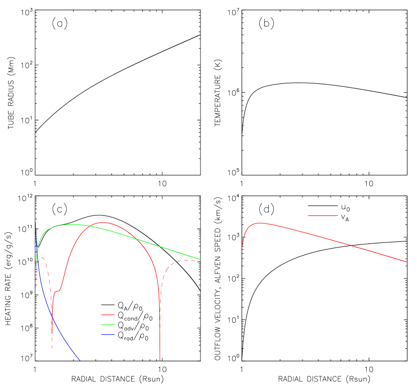
Figure 1: Radial dependence of various background quantities for Model A. (a) Flux tube radius. (b) Temperature. (c) Plasma heating rate due to wave dissipation (black curve), and energy-loss rates due to thermal conduction (red curve), advection (green curve), and radiation (blue curve). (d) Outflow velocity (black curve) and Alfvén speed (red curve).

Figure 1 shows the background atmosphere for Model A, which is nearly identical to the model described in section 3 of paper I. Figure 1(a) shows the flux tube radius $R(r)$, which increases from 6 Mm at the coronal base to 360 Mm at $r=20$ $R_{\odot}$. Figure 1(b) shows the assumed temperature $T_{0}(r)$, which is given by equation (59) of paper I with parameter values $C_{0}=0.35$, $C_{1}=2$, $m=0.3$ and $k=8$. Figure 1(c) shows the plasma heating rate $Q_{\rm A}(r)$ necessary to maintain this temperature. The heating is assumed to be balanced by cooling due to the expansion of the outflowing plasma ($Q_{\rm adv}$), radiative losses ($Q_{\rm rad}$) and conductive losses ($Q_{\rm cond}$); these contributions are shown by the colored curves in Figure 1(c). The dashed red curves indicate regions where $Q_{\rm cond}<0$, i.e., the convergence of the conductive flux is heating the plasma. Figure 1(d) shows the outflow velocity $u_{0}(r)$ and the Alfvén speed $v_{\rm A}(r)$. Note that the Alfvén critical point is located at $r\approx 7.2$ $R_{\odot}$.

On the real Sun Alfvén- and/or kink waves may be produced by interactions of photospheric magnetic elements with granule-scale convective flows (e.g., Spruit, 1982; Edwin & Roberts, 1983; Morton et al., 2013). Due to the density stratification of the lower atmosphere, the waves are significantly amplified on their way to the corona. However, the present model does not include the lower atmosphere, but starts at the coronal base. The waves are launched by imposing random “footpoint” motions on the plasma and magnetic field at the coronal base. The footpoint velocity is given by ${\bf v}=\nabla_{\perp}f\times\hat{\bf B}_{0}$, where $f(x,y,r_{\rm base},t)$ is the velocity stream function at the coronal base. The latter is written as a sum over basis functions:

$$f(x,y,r_{\rm base},t)=\sum_{k\in D}f_{k}(r_{\rm base},t)\tilde{F}_{k}(\tilde{x},\tilde{y}),$$ (19)

where $D$ is a set of “driver” modes with dimensionless wavenumbers in the range $3.5\pi<a_{k}<5.5\pi$. The amplitudes $f_{k}(r_{\rm base},t)$ of the driver modes vary randomly with time $t$ in the simulation. For each mode we first create a normally distributed random sequence $f(t)$ on a grid of times covering the entire simulation ($t_{\rm max}=$ 30,000 s). Then the sequence is Fourier filtered using a Gaussian function $G(\tilde{\nu})=\exp[-(\tau_{0}\tilde{\nu})^{2}]$, where $\tilde{\nu}$ is the temporal frequency (in Hz) and $\tau_{0}$ is a specified parameter. In the present work we use $\tau_{0}=120$ s, which corresponds to a correlation time $\tau_{\rm c}=\tau_{0}/\sqrt{2\pi}\approx 48$ s; this value was chosen to be comparable to the timescale of the solar granulation. The filtered sequences are renormalized such that each driver mode has an equal contribution to the square of the velocity:

$$\frac{a_{k}^{2}}{R_{\rm base}^{2}}<f_{k}^{2}>=\frac{v_{\rm rms,\odot}^{2}}{N_{D}},$$ (20)

where $<\cdots>$ denotes a statistical average, and $N_{D}$ is the number of driver modes ($N_{D}=60$). The driver modes are assumed to be uncorrelated, $<f_{l}f_{k}>=0$ for $l\neq k$. We assume $v_{\rm rms,\odot}=40$ $\rm km~{}s^{-1}$, consistent with the value used in the setup of the background model. This value is also consistent with observed spectral line widths and non-thermal velocities in coronal holes (Wilhelm et al., 1998; McIntosh et al., 2008; Banerjee et al., 2009; Landi & Cranmer, 2009; Singh et al., 2011; Hahn et al., 2012; Bemporad & Abbo, 2012). Note that the dynamical time of the footpoint motions is comparable to the correlation time, $\tau_{\rm dyn}=2\lambda_{\perp,\odot}/v_{\rm rms,\odot}=50$ s. The normalized autocorrelation function for the $x$-component of velocity is given by

$$C_{x}(\Delta x,\Delta y) \equiv \frac{<v_{x}(x+\Delta x,y+\Delta y,t)v_{x}(x,y,t)>}{<v_{x}^{2}>},$$ (21)

$$= \frac{2}{N_{D}}\sum_{k\in D}\frac{a_{y,k}^{2}}{a_{k}^{2}}\cos(a_{x,k}\Delta\tilde{x})\cos(a_{y,k}\Delta\tilde{y}),$$

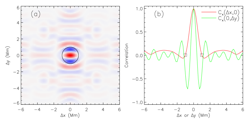
Figure 2: Autocorrelation function of the footpoint velocity $v_{x}(x,y,t)$ at the coronal base.

where $(\Delta x,\Delta y)$ are spatial offsets, and $(\Delta\tilde{x},\Delta\tilde{y})$ are dimensionless values of these offsets (normalized by $R_{\rm base}$). Figure 2(a) shows this correlation function as a color-scale plot. The anisotropy of the distribution is due to the fact that we consider here only the $x$-component of the velocity; the correlation function for $v_{y}(x,y,t)$ would be rotated by 90 degrees. Figure 2(b) shows two cross-sections of the correlation function, $C_{x}(\Delta x,0)$ (red curve) and $C_{x}(0,\Delta y)$ (green curve). The circle in Figure 2(a) indicates the region where the strongest (positive or negative) correlations are found. We use the radius of this circle as our definition of the autocorrelation length $\lambda_{\perp,\odot}$ of the footpoint motions. Note that $\lambda_{\perp,\odot}=1$ Mm, significantly smaller than the domain half-width, $R_{\rm base}=6$ Mm.

The present model neglects all details of the collisionless processes by which the waves are dissipated at small spatial scales. The “dissipation range” of the turbulence is defined as the region in wavenumber space where the simulated waves are dissipated. In the present model the dissipation range is given by $a_{k}>(2/3)a_{\rm max}$, where $a_{\rm max}$ is the maximum dimensionless wavenumber in the model. In the region below the dissipation range we set $\nu_{\pm,k}=0$, so that these waves can propagate over long distance without significant dissipation. Inside the dissipation range we use $\nu_{\pm,k}=\nu_{\pm}$, the same for all modes. The damping rate $\nu_{\pm}$ is twice the nonlinear cascade rate for those waves:

$$\nu_{\pm}=2k_{\rm d}Z_{\mp,\rm d},$$ (22)

where $k_{\rm d}=(2/3)a_{\rm max}/R$ is the wavenumber at the start of the dissipation range, and $Z_{\mp,\rm d}$ is the Elsasser variable just below this range. The latter is given by

$$Z_{\mp,\rm d}\equiv\sqrt{\sum_{i}(a_{i}/R)^{2}f_{\mp,i}^{2}},$$ (23)

where the sum is taken over all modes with wavenumbers in the range $(1/2)a_{\rm max}<a_{i}<(2/3)a_{\rm max}$. Note that the damping rate $\nu_{+}$ for the dominant waves depends on the Elsasser variable $Z_{-,\rm d}$ of the minority waves, and vice versa, so the damping rates satisfy $\nu_{+}\ll\nu_{-}$. This differs from the approach used in paper I where we assumed $\nu_{+}=\nu_{-}$. The present method has the advantage that the waves are dissipated at a rate comparable to the rate at which energy is injected into the dissipation range by cascade. We find that this approach produces wave energy spectra that are only weakly affected by the “bottleneck” effect (e.g. Beresnyak & Lazarian, 2009b).

The numerical methods for solving the RMHD equations (6) are mostly described in Appendix B of paper I, but there are some important differences. In paper I we assumed a circular cross-section, and the nonlinear terms were evaluated by summing over the nonzero elements of $M_{kji}$. As already mentioned, we now use a square domain and periodic boundary conditions. We use a set of modes with $n_{x,k}$ and $n_{y,k}$ in the range 0 to 21, so the maximum dimensionless wavenumber $a_{\rm max}=21\pi=65.97$, which is higher than the value $a_{\rm max}=30$ used in paper I. In the present case the total number of modes $k_{\rm max}=1848$, and there are about 7 million matrix elements with $M_{kji}\neq 0$. Instead of summing over mode triples, we evaluate the nonlinear terms using the Fast Fourier Transform (FFT) method (also see Perez & Chandran, 2013). In essence, the arrays $f_{\pm,k}$ are transformed into functions in real space $(\tilde{x},\tilde{y})$, and the brackets are then computed as described in equation (2). We verified that the FFT method for computing the brackets produces exactly the same result as explicitly summing over mode triples. The half-width $R_{\rm base}$ of the computational domain at the coronal base is 6 Mm, significantly larger than the correlation length of the footpoint motions, $\lambda_{\perp,\odot}=1$ Mm. The RMHD equations are still integrated with a time step $\Delta t_{0}=1$ s. The code is parallelized using OPENMP.

4 MODELS WITH A SMOOTH BACKGROUND ATMOSPHERE

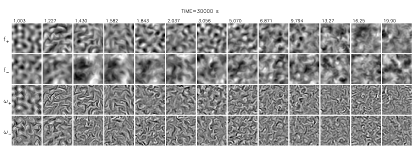
Figure 3: Velocity patterns of the Alfvén waves in cross-sections of the flux tube. Top rows: velocity stream functions $f_{\pm}(x,y)$ of dominant $(+)$ and minority $(-)$ waves. Bottom rows: parallel component of vorticity, $\omega_{\pm}(x,t)$ dominant and minority waves. The different columns correspond to different heights along flux tube. Each panel shows the normalized distribution of the relevant quantity.

In this section we first describe RMHD simulations for Model A, which has a smooth background atmosphere (see Figure 1). The Alfvén waves launched at the coronal base produce reflection-driven turbulence at larger heights. The outward-propagating waves first reach the outer boundary of the model ($r=20$ $R_{\odot}$) after about 10,859 s, and we simulate the turbulence for a period of 30,000 s. Figure 3 shows wave velocity patterns in cross sections of the flux tube at the end of the simulation. The first and second rows show the velocity stream functions $f_{\pm}(x,y)$, and the third and fourth rows show the vorticities $\omega_{\pm}(x,y)$. The different columns correspond to different positions along the tube and are labeled with the radial distance $r/R_{\odot}$. Each panel is normalized, so Figure 3 does not provide any quantitative information on the amplitude of the waves.

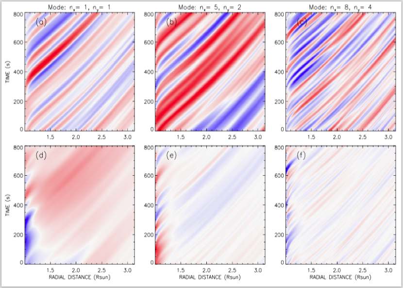
Figure 4: Vorticities $\omega_{\pm,k}(r,t)$ as function of radial distance $r$ and time $t$ for three different wave modes $k$ in Model A, which has a smooth background atmosphere.

Velli et al. (1989) predicted that the minority waves have both an inward-propagating “classical” component and an outward-propagating “anomalous” component. Figure 4 shows the vorticities $\omega_{\pm,k}(r,t)$ of the simulated waves plotted as function of radial distance $r$ and time $t$ for three different wave modes $k$. The selected modes have basis functions of the form $\tilde{F}_{k}(\tilde{x},\tilde{y})=2\cos(\pi n_{x,k}\tilde{x})\cos(\pi n_{y,k}\tilde{y})$, and the values of $n_{x,k}$ and $n_{y,k}$ are given at the top of each column of Figure 4. The upper panels show the dominant waves $\omega_{+,k}$, and the lower panels show the corresponding minority waves $\omega_{-,k}$. Note that the velocity patterns in the lower panels have the same positive slopes as the patterns in the upper panels. Therefore, the minority waves travel radially outward with the same velocity ($u_{0}+v_{\rm A}$) as the dominant waves. There is no evidence in these diagrams for inward-propagating waves with negative slopes, and the same is true for all wave modes in our simulation. This means that the minority waves are dominated by the “anomalous” component (also see Perez & Chandran, 2013, and paper I). Therefore, it is not correct to think of the minority waves as inward-propagating waves.

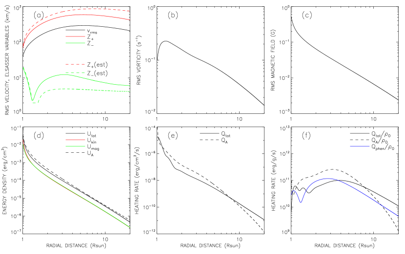
Figure 5: Radial dependence of various wave-related quantities: (a) Velocity amplitude of the waves (black curve), and Elsasser variables for dominant waves (red curve) and minority waves (green curve). The dashed red/green curves are estimates for the Elsasser variables. (b) Amplitude of the vorticity. (c) Amplitude of the fluctuating component of magnetic field. (d) Wave energy densities: total energy (black curve), kinetic energy (red curve), and magnetic energy (green curve). Also shown is the wave energy density assumed in setup of the background atmosphere (dashed curve). (e) Wave energy dissipation rates per unit volume: total wave dissipation rate $Q_{\rm tot}$ (solid black curve), and plasma heating rate $Q_{\rm A}$ assumed in setup of the background atmosphere (dashed black curve). (f) Wave energy dissipation rates per unit mass: rate derived from turbulence simulation (solid black curve), rate assumed in the setup of background atmosphere (dashed curve), and rate predicted by a phenomenological turbulence model (blue curve), equation (27) with $c_{\rm d}=0.1$.

Figure 5 shows various wave-related quantities averaged over the cross-section of the flux tube and over the time. Each quantity is averaged over the time interval $t_{0}(r)+300\leq t\leq 30000$ (in seconds), where $t_{0}(r)$ is the time for an outward propagating wave to reach a certain height:

$$t_{0}(r)\equiv\int_{r_{\rm base}}^{r}\frac{dr^{\prime}}{u_{0}(r^{\prime})+v_{\rm A}(r^{\prime})}.$$ (24)

The black curve in Figure 5(a) shows the rms velocity amplitude of the waves, $v_{\rm rms}(r)$. The solid red and green curves in Figure 5(a) show the rms values of the Elsasser variables, $Z_{\pm}(r)=\sqrt{<|{\bf z}_{\pm}|^{2}>}$. Note that the minority waves are much weaker than the dominant waves; at $r>5$ $R_{\odot}$ the ratio $Z_{-}/Z_{+}\approx 0.016$. The function $Z_{-}(r)$ has a sharp minimum at $r\approx 1.3$ $R_{\odot}$, which is due to the fact that the Alfvén speed has a maximum near that height, see Figure 1(d). Figure 5(b) shows the rms vorticity of the waves, which is dominated by waves with high perpendicular wavenumbers and therefore more sensitive to the spatial resolution of the model. Figure 5(c) shows the rms value of the magnetic fluctuations.

The numerical results for the Elsasser variables can be compared with predictions from a turbulence model that uses a simple phenomenology for the cascade and dissipation of waves (Chandran & Hollweg, 2009). This analytical model gives the following estimates (also see Chandran et al., 2011):

$$Z_{+,\rm est} = \frac{2v_{\rm rms,\odot}}{1+M_{\rm A}}\left(\frac{\rho_{0}}{\rho_{0,\rm base}}\right)^{-1/4},$$ (25)

$$Z_{-,\rm est} = (1+M_{\rm A})\lambda_{\perp}\left|\frac{dv_{\rm A}}{dr}\right|,$$ (26)

where $v_{\rm rms,\odot}$ is the velocity amplitude at the coronal base, $\rho_{0,\rm base}$ is the base density, $M_{\rm A}(r)\equiv u_{0}/v_{\rm A}$ is the Alfvén Mach number, and $\lambda_{\perp}(r)$ is the perpendicular correlation length of the turbulence. The latter is estimated by extrapolation from the coronal base: $\lambda_{\perp}(r)=\lambda_{\perp,\odot}[B_{0}(r)/B_{\rm base}]^{-1/2}$, where $\lambda_{\perp,\odot}=1$ Mm is the autocorrelation length of the footpoint velocity at the base, and $B_{\rm base}=10$ G is the field strength at the base. We further impose a minimum value on the Elsasser variable for the minority waves: $Z_{-,\rm est}>2$ $\rm km~{}s^{-1}$. The quantities $Z_{+,\rm est}$ and $Z_{-,\rm est}$ are plotted in Figure 5(a) as dashed red and green curves. Note that these estimates are accurate to about a factor of 2. Therefore, the model by Chandran & Hollweg (2009) indeed provides an approximate description of the Elsasser variables in the acceleration region of the wind.

Figure 5(d) shows the total energy density $U_{\rm tot}$ of the simulated waves (full black curve), together with the contributions from the kinetic energy $U_{\rm kin}$ (red curve) and magnetic energy $U_{\rm mag}$ (green curve). The dashed curve shows the wave energy density $U_{\rm A}$ used in the setup of the background model. We see that $U_{\rm kin}\approx U_{\rm mag}$ and $U_{\rm tot}\approx U_{\rm A}$, consistent with the assumptions made in the model setup (see paper I).

Figure 5(e) shows the total energy dissipation rate $Q_{\rm tot}(r)$ of the simulated turbulence (solid black curve). Unlike for the model of paper I, this rate is now dominated by the contribution from damping at high perpendicular wavenumbers, and the contribution from damping at high parallel wavenumbers is no longer significant (but still included). The dissipation rate $Q_{\rm tot}$ is higher than that found for the smooth model in paper I, even though the background atmospheres are nearly identical. This indicates that the results of paper I are to some degree affected by a numerical artifact, namely, a “bottleneck” effect that flattens the power spectrum (see Figure 3(a) of paper I) and reduces the cascade rate for the dominant waves. The dashed black curve in Figure 5(e) shows the plasma heating rate $Q_{\rm A}(r)$ used in the model setup. Note that $Q_{\rm tot}<Q_{\rm A}$ over a significant height range in the model. Therefore, the wave dissipation rate is still smaller than the plasma heating rate needed to sustain the background atmosphere, and the model is not in thermal equilibrium. Figure 5(f) shows the same wave dissipation and plasma heating rates per unit mass. We also compare our results with predictions from a “phenomenological” turbulence model (e.g., Zhou & Matthaeus, 1990; Hossain et al., 1995; Matthaeus et al., 1999; Dmitruk et al., 2001), which predicts that the dissipation rate $Q_{\rm phen}$ is given by

$$Q_{\rm phen}=c_{\rm d}\rho_{0}\frac{Z_{+}^{2}Z_{-}+Z_{-}^{2}Z_{+}}{4\lambda_{\perp}}.$$ (27)

Here $c_{\rm d}$ is a dimensionless factor of order unity. The blue curve in Figure 5(f) shows the quantity $Q_{\rm phen}/\rho_{0}$ as function of radial distance for $c_{\rm d}=0.1$. This value was chosen to obtain a crude fit to the actual dissipation rate $Q_{\rm tot}(r)$ predicted by the RMHD simulation. Without this correction factor the above expression would significantly overestimate the dissipation rate.

Figures 6(a) and 6(b) show power spectra for the Elsasser variables as function of dimensionless perpendicular wavenumber $a_{\perp}$ for four different heights in the model. For each height we compute the wave power in individual modes with wavenumbers $a_{k}$, and then collect the results into bins in wavenumber space with $\Delta a_{\perp}=2$ (for details see van Ballegooijen et al., 2011). These results are derived from the last 800 s of the simulation. Figure 6(a) shows the power spectra for the dominant waves. The waves are injected at $a_{\perp}\sim 15$, which corresponds to the correlation length $\lambda_{\perp,\odot}$ of the footpoint motions. Figure 6(b) shows similar spectra for the minority waves. In the present work both spectra have approximately the same slopes, which are similar to those found in high-resolution turbulence simulations (e.g., Beresnyak & Lazarian, 2008, 2009a, 2009b; Perez & Boldyrev, 2009; Perez et al., 2012; Perez & Chandran, 2013). We also compute temporal power spectra of dominant and minority waves, and derive the average wave frequency $\tilde{\omega}_{\pm}$ as function of dimensionless perpendicular wavenumber $a_{\perp}$. The results are shown in Figures 6(c) and 6(d) for four different heights in the model.

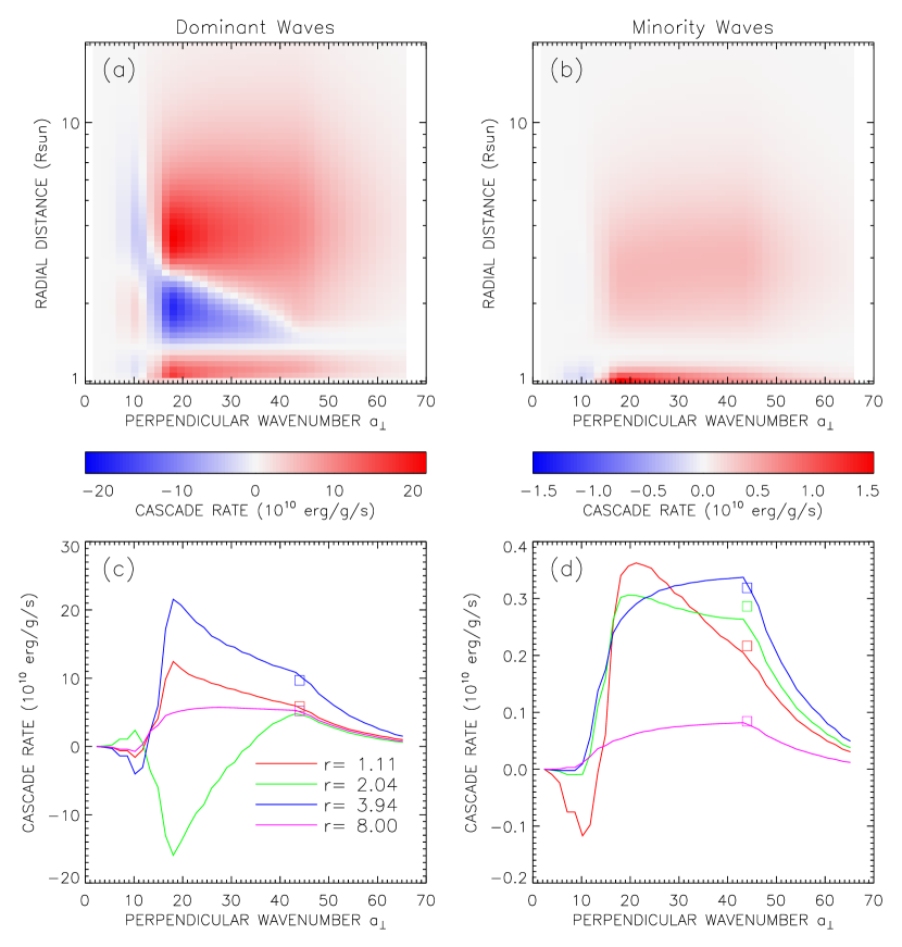
Figure 7: Energy cascade rates in the simulated turbulence for Model A. (a) Cascade rate per unit mass for the dominant waves, $\epsilon_{+}/\rho_{0}$, as function of dimensionless perpendicular wavenumber $a_{\perp}$ and radial distance $r$ from Sun center. Direct and inverse cascades are indicated by red and blue colors, respectively (see color bar). (b) Cascade rate per unit mass for the minority waves, $\epsilon_{-}/\rho_{0}$, with separate color bar. (c) Dominant cascade rates as function of $a_{\perp}$ for four different radial distances, as indicated by the legend. (d) Minority cascade rates at the same heights.

Figure 7 shows the time-averaged energy cascade rates per unit mass, $\epsilon_{\pm}/\rho_{0}$. These rates are functions of dimensionless perpendicular wavenumber $a_{\perp}$ and radial distance $r$. Figures 7(a) and 7(b) show color-scale plots for the dominant and minority waves, respectively. Note that each plot has its own color bar, and that the cascade rates for the dominant waves are much larger than those for the minority waves. Red and blue colors indicates direct ($\epsilon_{\pm}>0$) and inverse ($\epsilon_{\pm}<0$) cascades, respectively. Figure 7(a) shows that at low heights the dominant waves have a direct cascade, but $\epsilon_{+}$ changes sign at $r=1.4$ $R_{\odot}$ for wavenumbers in the range $15<a_{\perp}<44$. The lower boundary of this range ($a_{\perp}=15$) is approximately where energy is injected into the turbulence by the driver waves, and the upper boundary ($a_{\perp}=44$) is where the waves start to be dissipated. The inverse cascade continues up to $r=2.5$ $R_{\odot}$, but in a narrowing wavenumber range. These negative cascade rates reduce the amount of energy that can cascade into the dissipation range ($a_{\perp}>44$), and therefore affect the overall wave dissipation rate between 1.4 and 2.5 $R_{\odot}$. There is also a further extension of the region of inverse cascade to larger heights ($r>2.5$ $R_{\odot}$) and low perpendicular wavenumbers ($a_{\perp}<15$), but this feature is relatively weak and does not seem to have a strong effect on the dissipation rates. In contrast, Figure 7(b) shows that the minority waves have a direct cascade at all heights.

Figures 7(c) and 7(d) show plots of the cascade rates, $\epsilon_{\pm}/\rho_{0}$, as function of perpendicular wavenumber for four different heights. These heights were chosen to represent the region of direct cascade near the coronal base ($r=1.11$ $R_{\odot}$, red curves), the region of inverse cascade at intermediate heights ($r=2.04$ $R_{\odot}$, green curves), and the direct cascades at large heights ($r=3.94$ $R_{\odot}$, blue curves; $r=8.0$ $R_{\odot}$, magenta curves). The colored squares give the wave dissipation rates $Q_{\pm}/\rho_{0}$. The dissipation rates are approximately equal to the cascade rates at the start of the dissipation range ($a_{\perp}=44$), where the squares are plotted. Hence, the energy that cascades into the dissipation range is indeed dissipated shortly afterward, as expected. Note that at most heights the cascade rates vary strongly with wavenumber $a_{\perp}$, even in the “inertial” range ($15<a_{\perp}<44$) where no injection or dissipation of the energy occurs. This indicates that the transport of wave energy is a highly non-local process: as the waves cascade, they also propagate upward in height over a significant distance. This is due to the fact that the nonlinear cascade time for the dominant waves is comparable to the wave propagation time (see paper I).

What is the cause of the inverse cascade for the dominant waves? To answer this question we first consider the production of minority waves by “reflection” of dominant waves. Converting vorticities to mode amplitudes $f_{\pm,k}$ and using the fact that the minority waves are weak ($|f_{-,k}|\ll|f_{+,k}|$), equation (6) can be written as

$$\frac{\partial f_{-,k}}{\partial t}+(u_{0}-v_{\rm A})\frac{\partial f_{-,k}}{\partial r} \approx \text@onehalf(1+M_{\rm A})\frac{dv_{\rm A}}{dr}f_{+,k}$$ (28)

$$+\frac{1}{2R^{2}a_{k}^{2}}\sum_{j}\sum_{i}M_{kji}(a_{i}^{2}-a_{j}^{2}-a_{k}^{2})f_{-,j}f_{+,i},$$

where we omit the wave damping terms. Note that the “nonlinear” term in equation (28) is in fact linear in the amplitudes $f_{-,j}(r,t)$ of the minority waves. Also, the production of minority waves is proportional to the Alfvén speed gradient $dv_{\rm A}/dr$, which is positive at heights below the peak in Alfvén speed ($r<1.4$ $R_{\odot}$) and negative above the peak ($r>1.4$ $R_{\odot}$). The dominant waves have a long cascade time and evolve only gradually with height. However, the minority waves have a short cascade time (about 10 s at the outer scale of the turbulence, see paper I), and respond much more rapidly to the changes in $dv_{\rm A}/dr$ with height. Therefore, as the waves propagate outward through the region around the peak in Alfvén speed, the dominant waves $f_{+,k}(r,t)$ remain more or less unchanged, while the minority waves $f_{-,k}(r,t)$ change sign. This reversal of the minority waves at $r\approx 1.4$ $R_{\odot}$ occurs for most modes, and can be seen in diagrams such as Figure 4. The reversal occurs even when the dominant and minority waves are not well correlated with each other, as is the case at higher wavenumbers. We now consider two heights, one just below the peak in Alfvén speed ($r=r_{1}$) and another just above it ($r=r_{2}$), such that the magnitudes of the gradients are the same at the two heights: $(dv_{\rm A}/dr)_{2}=-(dv_{\rm A}/dr)_{1}$. The dominant and minority waves at these heights are approximately related by

$$f_{+,k}(r_{2},t) \approx f_{+,k}(r_{1},t-\Delta t_{12}),$$ (29)

$$f_{-,k}(r_{2},t) \approx -c_{0}~{}f_{-,k}(r_{1},t-\Delta t_{12}),$$ (30)

where $c_{0}\approx 1$ (independent of mode index $k$), and $\Delta t_{12}$ is the wave propagation time between the two heights. These relationships follow from a symmetry of equation (28): the equation remains valid when the signs of $dv_{\rm A}/dr$ and all $f_{-,k}$ are reversed, but $f_{+,k}$ is unchanged. Inserting expressions (29) and (30) into equation (18), we find the following relationships between the cascade rates at the two heights:

$$\epsilon_{+}(a_{\perp},r_{2}) \approx -c_{0}~{}\epsilon_{+}(a_{\perp},r_{1}),$$ (31)

$$\epsilon_{-}(a_{\perp},r_{2}) \approx c_{0}^{2}~{}\epsilon_{-}(a_{\perp},r_{1}).$$ (32)

Figure 7 indicates that at low heights there is a direct cascade for both wave types, $\epsilon_{\pm}(a_{\perp},r_{1})>0$. Then equations (31) and (32) predict that at $r=r_{2}$ there is an inverse cascade for the dominant waves and a direct cascade for the minority waves, $\epsilon_{+}(a_{\perp},r_{2})<0$ and $\epsilon_{-}(a_{\perp},r_{2})>0$. The inverse cascade of the dominant waves occurs at all wavenumbers $a_{\perp}$ because the reversal in sign of $f_{-,k}$ is rapidly transmitted to larger wavenumbers by the direct cascade of the minority waves.

As the dominant waves propagate farther out they gradually adjust to the condition $dv_{\rm A}/dr<0$, and $\epsilon_{+}$ becomes positive again. The adjustment of the dominant waves occurs first at large wavenumbers where the cascade times for the dominant waves are shortest, and later also at smaller wavenumbers. Therefore, in Figure 7(a) the upper boundary of the region with inverse cascade lies at an angle in the $(a_{\perp},r)$ plane. We conclude that the inverse cascade in Figure 7(a) is linked to the change of sign of $dv_{\rm A}/dr$ at $r=1.4$ $R_{\odot}$, together with the fact that the cascade time for the dominant waves is relatively large and comparable to the wave travel time $t_{0}(r)$.

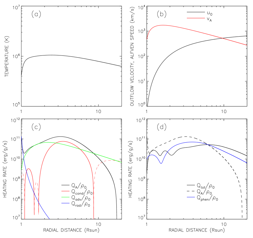
Figure 8: Background quantities and simulation results for Model B. (a) Temperature. (b) Outflow velocity (black curve) and Alfvén speed (red curve). (c) Plasma heating rate required to maintain the background atmosphere (black curve), and energy-loss rates due to thermal conduction (red curve), advection (green curve) and radiation (blue curve). (d) Wave energy dissipation rate as derived from the RMHD simulation (solid black curve), rate assumed in the setup of background atmosphere (dashed curve), and rate predicted by a phenomenological turbulence model (blue curve), equation (27) with $c_{\rm d}=0.1$.

The background atmosphere for Model A was chosen to be the same as that used in paper I, so we could directly compare our results and understand why the model of paper I gives such low wave dissipation rates. However, the outflow speed in this model reaches 800 $\rm km~{}s^{-1}$ by 20 $R_{\odot}$ (see Figure 1(d)), which is high considering that further acceleration may occur at larger radii. Also, the Alfvén critical point is located at 7.2 $R_{\odot}$, which is low compared to other models that rely on Alfvén waves to heat and accelerate the fast solar wind (e.g., Cranmer et al., 2007; Verdini et al., 2010; Chandran et al., 2011). Therefore, we now consider an alternative, Model B, which has a different set of model parameters. Three of the four parameters describing the background temperature were modified ($C_{0}=0.30$, $m=0.35$, $k=12$, see Appendix D in paper I), which leads to a reduction of the peak temperature from 1.31 MK to 1.05 MK. The revised temperature profile is shown in Figure 8(a). We also increased the coronal base pressure from 0.1 to 0.2 $\rm dyne~{}cm^{-2}$, and decreased the wave amplitude to $v_{\rm rms,\odot}=30$ $\rm km~{}s^{-1}$, which reduces the wave pressure acceleration. Figure 8(b) shows the outflow velocity $u_{0}(r)$ and Alfvén speed $v_{\rm A}(r)$ resulting from these changes. In Model B the peak in Alfvén speed occurs at $r\approx 1.6$ $R_{\odot}$, and the Alfvén critical point is located at $r=9.6$ $R_{\odot}$, more in line with the values used in earlier models. The plasma heating rate $Q_{\rm A}(r)$ needed to maintain the background temperature is shown by the black curve in Figure 8(c), together with the cooling rates due to radiation (blue curve), thermal conduction (red curve) and solar wind expansion (green curve). Comparison with Figure 1(c) for Model A shows that the heating rate is significantly reduced. In fact, at large radii $Q_{\rm A}$ becomes slightly negative, which is due to the near balance of conduction heating and expansion cooling at $r=20$ $R_{\odot}$ in Model B.

We simulated the dynamics of the Alfvén waves in Model B for a period of 30,000 s. The imposed footpoint motions are the same as in Model A. The full black curve in Figure 8(d) shows the time-averaged wave dissipation rate $Q_{\rm tot}(r)$, and the blue curve shows the rate $Q_{\rm phen}(r)$ predicted by the phenomenological turbulence model, equation (27) with $c_{\rm d}=0.1$. Note that the wave dissipation rate $Q_{\rm tot}$ is reduced compared to Model A, and is below the required heating rate $Q_{\rm A}$ (dashed curve) for $1.5<r<5$ $R_{\odot}$. This is again due to the presence of an inverse cascade, in this case in the height range $1.6<r<4$ $R_{\odot}$. The heating produced by the waves is insufficient to maintain the assumed background temperature, so the model is not in thermal equilibrium.

5 MODEL WITH DENSITY VARIATIONS

In this section we describe simulation results for Model C, which has a background atmosphere with additional density variations along the flux tube. These variations simulate the effect that compressive MHD waves may have on the propagation and reflection of Alfvén waves. The density variations $\delta\rho_{0}(r)$ are assumed to be random in position, but constant in time, consistent with our RMHD methodology. The present model is similar to that described in section 4 of paper I, but the model parameters are different. The magnitude of the density variations has been doubled (to $\epsilon_{\rm rms}=0.2$), and the correlation length of the variations has been increased by a factor 5 (to $\lambda_{\rm c}=0.2$ $R_{\odot}$). Therefore, the magnitude of the variations in Alfvén speed gradient $dv_{\rm A}/dr$ has decreased by a factor 2.5, reducing the wave reflection. The main reason for these changes is to bring out more clearly the spatial variations of the cascade rates $\epsilon_{\pm}$ of the dominant- and minority waves. In reality there are density fluctuations both along and perpendicular to the field lines, and the latter may actually be much larger than the former (see references in section 4 of paper I). We believe that perpendicular density fluctuations will have an important effect on the cascade rates, but unfortunately we are unable to simulate this effect with our RMHD code, which assumes constant density over the cross-section of the flux tube. To compensate, we use a high value for the magnitude of the density fluctuations along the field lines. This approach is rather artificial, but it is the best we can do right now.

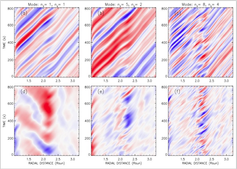
Figure 9: Vorticities $\omega_{\pm,k}(r,t)$ as function of radial distance $r$ and time $t$ for three different wave modes $k$ in Model C with random density variations.

In model C the Alfvén speed gradient $dv_{\rm A}/dr$ changes sign multiple times with increasing $r$, which significantly enhances the wave reflection. Figure 9 shows the vorticities $\omega_{\pm,k}(r,t)$ for three different wave modes, the same modes as in Figure 4. The upper panels of Figure 9 show the dominant waves $\omega_{+,k}$, and the lower panels show the corresponding minority waves $\omega_{-,k}$. The positive slopes in the upper panels indicate that the dominant waves travel radially outward with velocity $u_{0}+v_{\rm A}$. However, the velocity patterns in Figure 9(d) have negative slope, indicating this low-wavenumber minority wave ($a_{k}=4.44$) is propagating radially inward with velocity $u_{0}-v_{\rm A}<0$; this is the “classical” component of the minority waves described by Velli et al. (1989). In Figures 9(e) and 9(f) the minority waves have mostly outward-propagating components. All panels show a stationary (vertical) pattern, which is an artifact of our assumption that the density variations $\delta\rho_{0}(r)$ are constant in time. At high wavenumbers the minority waves are uncorrelated with the dominant waves (compare Figures 9(f) and 9(c)). These patterns are quite different from those for the smooth Model A (see Figure 4).

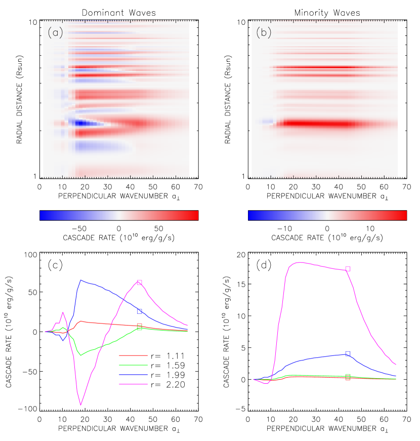
Figure 10: Energy cascade rates in the simulated turbulence for Model C. (a) Cascade rate per unit mass for the dominant waves, $\epsilon_{+}/\rho_{0}$, as function of dimensionless perpendicular wavenumber $a_{\perp}$ and radial distance $r$ from Sun center. Direct and inverse cascades are indicated by red and blue colors, respectively (see color bar). (b) Cascade rate per unit mass for the minority waves, $\epsilon_{-}/\rho_{0}$, with separate color bar. (c) Dominant cascade rates as function of $a_{\perp}$ for four different radial distances, as indicated by the legend. (d) Minority cascade rates at the same heights.

Figure 10 shows the time-averaged cascade rates $\epsilon_{\pm}(a_{\perp},r)$ for the model with density variations. Figure 10(a) shows the cascade rate $\epsilon_{+}/\rho_{0}$ for the dominant waves. Note that with increasing height $r$ the cascade rate changes sign multiple times, going from a direct cascade (red) to inverse cascade (blue) over short distances. In contrast, the minority waves always have a direct cascade, see Figure 10(b). The changes in $\epsilon_{+}$ as function of $r$ are due to changes in $dv_{\rm A}/dr$, but the dominant waves try to adjust to these changes, so at heights above 3 $R_{\odot}$ the quantities $\epsilon_{+}$ and $dv_{\rm A}/dr$ are only poorly correlated. Comparison of the color bars in Figures 7 and 10 indicate that the magnitudes of the cascade rates in Model C are much larger than those in Model A. Figures 10(c) and 10(d) show the cascade rates $\epsilon_{\pm}/\rho_{0}$ as functions of wavenumber for four different heights. The colored squares indicate the wave dissipation rates $Q_{\pm}/\rho_{0}$. Note that for the dominant waves the cascade rates vary strongly with wavenumber, and the dissipation rates $Q_{+}$ are much smaller than the peak cascade rates $|\epsilon_{+}|_{\rm max}$, which generally occur at low wavenumber. This indicates that the rapid changes in $\epsilon_{+}$ as function of $r$ prevent the efficient cascade of wave energy to higher wavenumbers, and thereby have a negative effect on the dissipation rate. The total dissipation rate $Q_{\rm tot}(r)$ for Model C is slightly larger than that for Model A, but is still insufficient to maintain the temperature of the background atmosphere. Therefore, Model C is also not in thermal equilibrium.

6 DISCUSSION AND CONCLUSIONS

In this work we simulate the dynamics of Alfvén waves for three models of the fast solar wind, two with a smooth background atmosphere (Models A and B) and one with density fluctuations (Model C). These models are improved versions of the models presented in paper I. We compute for the first time the energy cascade rates $\epsilon_{\pm}(a_{\perp},r)$ for dominant and minority waves, and find that at certain heights and wavenumbers the dominant waves undergo an inverse cascade, $\epsilon_{+}<0$. This means that the nonlinear interactions between dominant and minority waves cause energy to be transported from smaller to larger scales, opposite to the direction usually assumed for Alfvén wave turbulence. Inverse cascades are predicted to occur in two-dimensional magneto-hydrodynamic systems (Fyfe & Montgomery, 1976; Fyfe et al., 1977), and in three-dimensional systems with large magnetic helicity (Frisch et al., 1975; Dmitruk & Matthaeus, 2007). In the present case the inverse cascade appears to be due to a different mechanism, namely, the change in sign of the gradient of the Alfvén speed $dv_{\rm A}/dr$ as function of height in the model. In Model A the inverse cascade occurs for radii between 1.4 to 2.5 $R_{\odot}$ and wavenumbers in the inertial range ($15<a_{\perp}<44$); in Model B the inverse cascade occurs between 1.6 to 4 $R_{\odot}$. In Model C with density fluctuations the cascade rate changes sign multiple times as function of height. In all models the cascade rate $\epsilon_{+}(a_{\perp},r)$ varies significantly with perpendicular wavenumber. This indicates that wave propagation plays an important role in the cascade process. The cascade time scale for the dominant waves is comparable to the wave travel time $t_{0}(r)$, so in one cascade time the waves travel a distance comparable to the radial distance $r$. The energy injected into the cascade by the driver waves at position $r$ is not dissipated locally, but is dissipated only much later at significantly larger heights. Therefore, the cacsade of the dominant waves is a highly non-local process.

The inverse cascade impedes the efficient transport of wave energy to large perpendicular wavenumbers, and thereby has a negative effect on the wave dissipation rate. Therefore, the low dissipation rates found here (and in paper I) are a real physical effect, not a numerical artifact. In both the smooth models and the model with density fluctuations there is a significant height range where $Q_{\rm tot}(r)$ is less than the plasma heating rate $Q_{\rm A}(r)$ needed to maintain the temperature of the background atmosphere. Hence, these models are not self-consistent from an energy point of view. To obtain a model with higher dissipation rates would require that the inverse cascade is somehow avoided, or at least reduced in magnitude. At present it is unclear how to construct such a model.

In the smooth models the total dissipation rate $Q_{\rm tot}(r)$ is much lower than expected from a “phenomenological” turbulence model, equation (27) with $c_{\rm d}=1$. The phenomenological model is based on the assumption that the cascade rates $\epsilon_{\pm}(r,a_{\perp})$ are approximately constant with wavenumber $a_{\perp}$ in the inertial range, and that the cascade is everywhere direct. These assumptions are reasonable for a fully developed turbulent system in a closed box or periodic domain, but they are not appropriate for the extended corona where the cascade time for the dominant waves is comparable to the wave travel time and the dissipation is highly non-local. Indeed, we find that the cascade rate $\epsilon_{+}$ varies significantly with wavenumber in the inertial range. This fact prevents the straightforward application of the phenomenological formalism.

We predict that for models with a monotonically decreasing Alfvén speed $v_{\rm A}(r)$ a direct cascade rate occurs at all heights. To verify this prediction we constructed a model (not shown) with a temperature $T_{0}(r)$ that decreases monotonically with height. The model was constructed by setting $C_{0}=0.3$, $C_{1}=-2$ and $k=4$ in equation (59) of paper I; the coronal base pressure was assumed to be $0.03$ $\rm dyne~{}cm^{-2}$. In this model the Alfvén speed $v_{\rm A}(r)$ decreases monotonically with height. We find that indeed the cascade rate $\epsilon_{+}>0$ at all heights for wavenumbers larger than those of the driver waves ($a_{\perp}>15$). However, such a model for $v_{\rm A}(r)$ is not realistic. In the chromospheric-corona transition region the temperature $T_{0}(r)$ must increase with height, and the density must rapidly decrease, leading to a local increase in Alfvén speed $v_{\rm A}(r)$ with height. In the corona we expect high Alfvén speeds, $v_{\rm A}\sim 1000$ $\rm km~{}s^{-1}$. In the solar wind the Alfvén speed is again relatively low, $v_{\rm A}\sim 30$ $\rm km~{}s^{-1}$ at 1 AU. Therefore, for a realistic model of the fast solar wind the Alfvén speed $v_{\rm A}(r)$ must have a maximum at some height in the corona. Hence, inverse cascade of the kind found in the present models cannot easily be avoided.

The models presented here and in paper I differ significantly from other models in which the driver waves at the coronal base are assumed to have large perpendicular correlation lengths (10 to 30 Mm) and long correlation times (tens of minutes or longer) (e.g., Verdini et al., 2009; Perez & Chandran, 2013). Such large length and time scales are comparable to those of the supergranulation, which is a convective flow pattern observed in the solar photosphere. Long-period waves are more strongly reflected in the extended corona, and produce stronger minority waves and higher wave dissipation rates than the present model. However, as argued in paper I we do not believe that the supergranulation can play a significant role in producing the transverse waves that drive the solar wind. The reason is that supergranular flows have low velocity ($\sim 0.3$ $\rm km~{}s^{-1}$), and the magnetic elements in the lower atmosphere respond quasi-statically to such weak, slowly varying flows. The buoyant magnetic flux elements in the photosphere are expected to be passively advected by these horizontal flows without much amplification of the motions with increasing height. Therefore, the supergranular flows are expected to produce velocities of only about 0.3 $\rm km~{}s^{-1}$ in the low corona, not the much larger velocities assumed by Verdini et al. (2009) and Perez & Chandran (2013).

In contrast, in the present model the waves are asumed to be produced by interactions of magnetic elements with the solar granulation, which is a different convective pattern with a typical length scale of 1 Mm and time scale of a few minutes. The magnetic structures in the lower atmosphere respond dynamically to such short-period disturbances (e.g., van Ballegooijen et al., 2014), producing transverse waves that are amplified from about 1 $\rm km~{}s^{-1}$ in the photosphere to about 30 $\rm km~{}s^{-1}$ in the low corona. Therefore, in the present model we assume a relatively small correlation length ($\lambda_{\perp,\odot}=1$ Mm) and a short correlation time ($\tau_{\rm c}=50$ s). This produces less wave reflection than in models with long-period waves, and we find that the minority waves are predominantly of the outward-propagaing “anomalous” type, whereas Verdini et al. (2009) find that for long-period driving there is also a significant component of inward-propagating “classical” waves. Although we find an inverse cascade, its effects are limited to length scales smaller than those of the driver waves, and we do not find a strong tendency for the turbulence to cascade to larger scales. To distinguish between the different turbulence models will require further observations of Alfvén waves in coronal holes, including their typical length- and time scales and the relative amplitudes of outward- and inward-propagating waves. The observations by Morton et al. (2015) are an important step in that direction.

A number of authors have suggested that density fluctations and coupling between Alfvén- and compressive MHD waves play an important role in the heating of the fast solar wind (e.g., Kudoh & Shibata, 1999; Moriyasu et al., 2004; Suzuki & Inutsuka, 2005, 2006; Matsumoto & Shibata, 2010). Here we find that RMHD models with fixed density variations in the background atmosphere have inverse cascades that limit the rate at which wave energy can be dissipated. In such models sufficient energy is available at large spatial scales, but the energy is not efficiently cascaded to small scales where it can be dissipated. To obtain a more efficient cascade process it may be necessary to go beyond standard RMHD modeling and include the effects of perpendicular density variations, which give rise to phase mixing and resonant absorption of the waves (e.g., Heyvaerts & Priest, 1983; De Groof & Goossens, 2002; Goossens et al., 2011, 2012, 2013; Pascoe et al., 2012). Future modeling of Alfvén wave turbulence in the acceleration region of the fast wind should take such transverse density variations into account.

Figure 6: Spatial power spectra and wave frequencies as function of dimensionless perpendicular wavenumber $a_{\perp}$ for four different heights in the model. (a) Power spectra for the Elsasser variable of the dominant waves. The sharp drop at $a_{\perp}=44$ is due to the onset of $\nu_{+,k}$-damping at that wavenumber. (b) Power spectra for the Elsasser variable of the minority waves. (c) Average wave frequencies for dominant waves. (d) Average wave frequencies for minority waves. The different curves correspond to different heights as indicated in panel (b).

References

- Asgari-Targhi & van Ballegooijen (2012) Asgari-Targhi, M., & van Ballegooijen, A.A. 2012, ApJ, 746, 81
- Asgari-Targhi et al. (2013) Asgari-Targhi, M., van Ballegooijen, A.A., Cranmer, S.R., & DeLuca, E.E. 2013, ApJ, 773, 111
- Asgari-Targhi et al. (2014) Asgari-Targhi, M., van Ballegooijen, & Imada, S. 2014, ApJ, 786, 28
- Bale et al. (2005) Bale, S. D., Kellogg, P. J., Mozer, F. S., Horbury, T. S., & Reme, H. 2005, Phys. Rev. Letters, 94, 215002
- Banerjee et al. (2009) Banerjee, D., Pérez-Suárez, D., & Doyle, J. G. 2009, A&A, 501, L15
- Barnes (1966) Barnes, A. 1966, PhFl, 9, 1483
- Belcher (1971) Belcher, J.W. 1971, ApJ, 168, 509
- Belcher & Davis (1971) Belcher, J. W., & Davis, L., Jr. 1971, JGR, 76, 3534
- Bemporad & Abbo (2012) Bemporad, A., & Abbo, L. 2012, ApJ, 751, 110
- Beresnyak & Lazarian (2008) Beresnyak, A., & Lazarian, A. 2008, ApJ, 682, 1070
- Beresnyak & Lazarian (2009a) Beresnyak, A., & Lazarian, A. 2009a, ApJ, 702, 460
- Beresnyak & Lazarian (2009b) Beresnyak, A., & Lazarian, A. 2009b, ApJ, 702, 1190
- Bhattacharjee & Ng (2001) Bhattacharjee, A., & Ng, C. S. 2001, ApJ, 548, 318
- Borovsky (2012) Borovsky, J. E. 2012, J. Geophys. Res., 117, A05104
- Buchlin & Velli (2007) Buchlin, E., & Velli, M. 2007, ApJ, 662, 701
- Chandran (2005) Chandran, B. D. G. 2005, Phys. Rev. Lett., 95, 265004
- Chandran et al. (2011) Chandran, B. D. G., Dennis, T. J., Quataert, E., & Bale, S. D. 2011, ApJ, 743, 197
- Chandran & Hollweg (2009) Chandran, B. D. G., & Hollweg, J. V. 2009, ApJ, 707,1659
- Chandran et al. (2009) Chandran, B. D. G., Quataert, E., Howes, G. G., Hollweg, J. V., & Dorland, W. 2009, ApJ, 701, 652
- Cho et al. (2002) Cho, J., Lazarian, A., & Vishniac, E. T. 2002, ApJ, 564, 291
- Coburn et al. (2014) Coburn, J. T., Smith, C. W., Vasquez, B. J., Forman, M. A., & Stawarz, J. E. 2014, ApJ, 786, 52
- Coleman (1968) Coleman, P. J., Jr. 1968, ApJ, 153, 371
- Cranmer et al. (2015) Cranmer, S.R., Asgari-Targhi, M., Miralles, M. P., Raymond, J. C., Strachan, L., Tian, H., & Woolsey, L. N. 2015, Phil. Trans. Royal Soc. A, 373, 20140148
- Cranmer & van Ballegooijen (2005) Cranmer, S. R., & van Ballegooijen, A. A. 2005, ApJS, 156, 265
- Cranmer & van Ballegooijen (2012) Cranmer, S. R., & van Ballegooijen, A. A. 2012, ApJ, 745, 92
- Cranmer et al. (2007) Cranmer, S.R., van Ballegooijen, A.A., & Edgar, R.J. 2007, ApJS, 171, 520
- De Groof & Goossens (2002) De Groof, A., & Goossens, M. 2002, A&A, 386, 691
- De Pontieu et al. (2007) De Pontieu, B., McIntosh, S. W., Carlsson, M., et al. 2007, Sci, 318, 1574
- Dmitruk & Matthaeus (2003) Dmitruk, P., & Matthaeus, W. H. 2003, ApJ, 597, 1097
- Dmitruk & Matthaeus (2007) Dmitruk, P., & Matthaeus, W. H. 2007, Phys. Rev. E, 76, 036305
- Dmitruk et al. (2002) Dmitruk, P., Matthaeus, W. H., Milano, L. J., et al. 2002, ApJ, 575, 571
- Dmitruk et al. (2001) Dmitruk, P., Milano, L. J., & Matthaeus, W. H. 2001, ApJ, 548, 482
- Edwin & Roberts (1983) Edwin, P. M., & Roberts, B. 1983, Sol. Phys., 88, 179
- Elsasser (1950) Elsasser, W. M. 1950, Phys. Rev., 79, 183
- Frisch et al. (1975) Frisch, U., Pouquet, A., Léorat, J., & Mazure, A. 1975, J. Fluid Mech., 68, 769
- Fyfe & Montgomery (1976) Fyfe, D., & Montgomery, D. 1976, J. Plasma Phys., 16, 181
- Fyfe et al. (1977) Fyfe, D., Montgomery, D., & Joyce, G. 1977, J. Plasma Phys., 17, 369
- Goldreich & Sridhar (1995) Goldreich, P., & Sridhar, S. 1995, ApJ, 438, 763
- Goldreich & Sridhar (1997) Goldreich, P., & Sridhar, S. 1997, ApJ, 485, 680
- Goossens et al. (2012) Goossens, M., Andries, J., Soler, R., et al. 2012, ApJ, 753, 111
- Goossens et al. (2011) Goossens, M., Erdélyi, R., Ruderman, M.S. 2011, Space Sci. Rev., 158, 289
- Goossens et al. (2013) Goossens, M., Van Doorsselaere, T., Soler, R., & Verth, G. 2013, ApJ, 768, 191
- Grappin et al. (1982) Grappin, R., Frisch, U., Léorat, J., & Pouquet, A. 1982, A&A, 105, 6
- Grappin et al. (1983) Grappin, R., Pouquet, A., & Léorat, J. 1983, A&A, 126, 51
- Hahn et al. (2012) Hahn, M., Landi, E., & Savin, D. W. 2012, ApJ, 753, 36
- Heinemann & Olbert (1980) Heinemann, M., & Olbert, S. 1980, JGR, 85, 1311
- Heyvaerts & Priest (1983) Heyvaerts, J., & Priest, E.R. 1983, A&A, 117, 220
- Hollweg & Isenberg (2007) Hollweg, J. V., & Isenberg, P. A. 2007, JGR, 112, CiteID A08102
- Hollweg (1973) Hollweg, J. V. 1973, ApJ, 181, 547
- Hollweg (1986) Hollweg, J. V. 1986, J. Geophys. Res., 91, 4111
- Hollweg et al. (1982) Hollweg, J. V., Jackson, S., & Galloway, D. 1982, Sol. Phys., 75, 35
- Hossain et al. (1995) Hossain, M., Gray, P. C., Pontius, D. H., Jr., Matthaeus, W. H., & Oughton, S. 1995, Phys. Fluids, 7, 2886
- Iroshnikov (1963) Iroshnikov, P. S. 1963, Astron. Zh., 40, 742 (English translation in Sov. Astron. 7, 566 [1964])
- Jacques (1977) Jacques, S.A. 1977, ApJ, 215, 942
- Kraichnan (1965) Kraichnan, R. H. 1965, Phys. Fluids, 8, 1385
- Kudoh & Shibata (1999) Kudoh, T., & Shibata, K. 1999, ApJ, 514, 493
- Landi & Cranmer (2009) Landi, E., & Cranmer, S. R. 2009, ApJ, 691, 794
- Lionello et al. (2014) Lionello, R., Velli, M., Downs, C., Linker, J. A., & Mikić, Z. 2015, ApJ, 796, 111
- Liu et al. (2015) Liu, J., McIntosh, S. W., De Moortel, I., & Wang, Y. 2015, ApJ, 806, article id. 273
- Maron & Goldreich (2001) Maron, J., & Goldreich, P. 2001, ApJ, 554, 1175
- Marsch & Tu (1997) Marsch, E., & Tu, C.-Y. 1997, A&A, 319, L17
- Matsumoto & Shibata (2010) Matsumoto, T., & Shibata, K. 2010, ApJ, 710, 1857
- Matthaeus et al. (1990) Matthaeus, W. H., Goldstein, M. L., & Roberts, D. A. 1990, JGR, 95, 20673
- Matthaeus et al. (1999) Matthaeus, W. H., Zank, G. P., Oughton, S., Mullan, D. J., & Dmitruk, P. 1999, ApJ, 523, L93
- McIntosh et al. (2008) McIntosh, S. W., De Pontieu, B., & Tarbell, T. D. 2008, ApJ, 673, L219
- Moriyasu et al. (2004) Moriyasu, S., Kudoh, T., Yokoyama, T., & Shibata, K. 2004, ApJ, 601, L107
- Morton et al. (2015) Morton, R. J., Tomczyk, S., & Pinto, R. 2015, Nat. Comm., DOI: 10.1038/ncomms8813
- Morton et al. (2013) Morton, R. J., Verth, G., Fedun, V., Shelyag, S., & Erdélyi, R. 2013, ApJ, 768, 17
- Oran et al. (2013) Oran, R., van der Holst, B., Landi, E., Jin, M., Sokolov, I. V. & Gombosi, T. I. 2013, ApJ, 778, 176
- Oran et al. (2015) Oran, R., Landi, E., van der Holst, B., Lepri, S. T., Vásquez, A. M., et al. 2015, ApJ, 806, 55
- Oughton et al. (2001) Oughton, S., Matthaeus, W. H., Dmitruk, P., Milano, L. J., Zank, G. P., & Mullan, D. J. 2001, ApJ, 551, 565
- Parker (1965) Parker, E. N. 1965, Space Sci. Rev., 4, 666
- Pascoe et al. (2012) Pascoe, D. J., Hood, A. W., de Moortel, I., & Wright, A. N. 2012, A&A, 539, A37
- Perez & Boldyrev (2009) Perez, J. C., & Boldyrev, S. 2009, Phys. Rev. Letters, 102, 025003
- Perez & Chandran (2013) Perez, J. C., & Chandran, B. D. G. 2013, ApJ, 776, 124
- Perez et al. (2012) Perez, J. C., Mason, J., Boldyrev, S., & Cattaneo, F. 2012, Phys. Rev. X, 2, 041005
- Shebalin et al. (1983) Shebalin, J. V., Matthaeus, W. H., & Montgomery, D. 1983, J. Plasma Phys., 29, 525
- Singh et al. (2011) Singh, J., Hasan, S. S., Gupta, G. R., Nagaraju, K., & Banerjee, D. 2011, Sol. Phys., 270, 213
- Sokolov et al. (2013) Sokolov, I. V., van der Holst, B., Oran, R., Downs, C., Roussev, I. I., Jin, M., et al. 2013, ApJ, 764, 23
- Spruit (1982) Spruit, H. C. 1982, Sol. Phys., 75, 3
- Stawarz et al. (2009) Stawarz, J. E., Smith, C. W., Vasquez, B. J., Forman, M. A., & MacBride, B. T. 2009, ApJ, 697, 1119
- Strauss (1976) Strauss, H.R. 1976, Phys. Fluids, 19, 134
- Strauss (1997) Strauss, H. R. 1997, J. Plasma Phys., 57, 83
- Suzuki & Inutsuka (2005) Suzuki, T.K., & Inutsuka, S.-I. 2005, ApJ, 632, L49
- Suzuki & Inutsuka (2006) Suzuki, T.K., & Inutsuka, S.-I. 2006, J. Geophys. Res., 111, A6, CiteID A06101
- Threlfall et al. (2013) Threlfall, J., De Moortel, I., McIntosh, S. W., & Bethge, C. 2013, A&A, 556, A124
- Tian et al. (2014) Tian, H., DeLuca, E. E., Cranmer, S. R., et al. 2014, Science, 346, 1255711
- Tian et al. (2011) Tian, H., McIntosh, S. W., Habbal, S. R., He, J. 2011, ApJ, 736, 130
- Tomczyk & McIntosh (2009) Tomczyk, S., & McIntosh, S. W. 2009, ApJ, 697, 1384
- Tomczyk et al. (2007) Tomczyk, S., McIntosh, S. W., Keil, S. L., et al. 2007, Sci, 317, 1192
- Velli (1993) Velli, M. 1993, A&A, 270, 304
- Velli et al. (1989) Velli, M., Grappin, R., & Mangeney, A. 1989, Phys. Rev. Letters, 63, 1807
- Verdini et al. (2012) Verdini, A., Grappin, R., Pinto, R., & Velli, M. 2012, ApJ, 750, L33
- Verdini & Velli (2007) Verdini, A., & Velli, M. 2007, ApJ, 662, 669
- Verdini et al. (2009) Verdini, A., Velli, M., & Buchlin, E. 2009, ApJ, 700, L39
- Verdini et al. (2010) Verdini, A., Velli, M., Matthaeus, W. H., Oughton, S., & Dmitruk, P. 2010, ApJ, 708, L116
- van Ballegooijen et al. (2016) van Ballegooijen, A. A., & Asgari-Targhi, M. 2016, ApJ, 821, 106 (paper I)
- van Ballegooijen et al. (2014) van Ballegooijen, A. A., Asgari-Targhi, M., & Berger, M. A. 2014, ApJ, 787, 87
- van Ballegooijen et al. (2011) van Ballegooijen, A. A., Asgari-Targhi, M., Cranmer, S. R., & DeLuca, E. E. 2011, ApJ, 736, article 3
- van der Holst et al. (2014) van der Holst, B., Sokolov, I. V., Meng, X., et al. 2014, ApJ, 782, 81
- Wilhelm et al. (1998) Wilhelm, K., Marsch, E., Dwivedi, B. N., Hassler, D. M., Lemaire, Ph., Gabriel, A. H., & Huber, M. C. E. 1998, ApJ, 500, 1023
- Woolsey & Cranmer (2015) Woolsey, L. N., & Cranmer, S. R. 2015, ApJ, 811, 136
- Zhou & Matthaeus (1990) Zhou, Y., & Matthaeus, W. H. 1990, J. Geophys. Res., 95, 10291