Complete spin and orbital evolution of close-in bodies using a Maxwell viscoelastic rheology

Abstract

In this paper, we present a formalism designed to model tidal interaction with a viscoelastic body made of Maxwell material. Our approach remains regular for any spin rate and orientation, and for any orbital configuration including high eccentricities and close encounters. The method is to integrate simultaneously the rotation and the position of the planet as well as its deformation. We provide the equations of motion both in the body frame and in the inertial frame. With this study, we generalize preexisting models to the spatial case and to arbitrary multipole orders using a formalism taken from quantum theory. We also provide the vectorial expression of the secular tidal torque expanded in Fourier series. Applying this model to close-in exoplanets, we observe that if the relaxation time is longer than the revolution period, the phase space of the system is characterized by the presence of several spin-orbit resonances, even in the circular case. As the system evolves, the planet spin can visit different spin-orbit configurations. The obliquity is decreasing along most of these resonances, but we observe a case where the planet tilt is instead growing. These conclusions derived from the secular torque are successfully tested with numerical integrations of the instantaneous equations of motion on HD 80606 b. Our formalism is also well adapted to close-in super-Earths in multiplanet systems which are known to have non-zero mutual inclinations.

1 Introduction

Short period exoplanets are tidally distorted by their stars. This phenomenon alter both the planet rotation and its orbital evolution over long timescale. The mechanism is the same as in the problem of a satellite orbiting a planet which has been modeled by Darwin (1880) and generalized by Kaula (1964).

In these models, the gravitational potential of the deformed planet is expanded in multipoles and then expressed in terms of elliptical elements as a Fourier series truncated in eccentricity. Each term involves a Love number associated to the amplitude of the tide and a phase lag accounting for the non-instantaneous deformation of the planet. These lags have been interpreted as constant geometric lag angles (MacDonald, 1964). However, the tidal torque should vanish at equilibrium, i.e. when the perturbing body (star or satellite) has a circular orbit in the planet equatorial plane with a mean motion equal to the planet rotation speed. To remedy this problem, Singer (1968) proposed a frequency-dependent theory of tides which is now known as the constant time lag model. According to this theory, the deformation of the planet at time $t$ is aligned with the position occupied by the disturbing body at time $t-\Delta t$ in the planet reference frame.

The constant time lag model has been widely used because of its intuitive physical interpretation and also because the analytical expressions of the tidal force and torque expanded in first order in $\Delta t$ are very compact and not truncated in eccentricity (Mignard, 1979).

More generally, Love numbers and phase lags depend on the structure and the rheology of the planet (e.g., Efroimsky, 2012a), but none of the two models quoted above corresponds to a physical rheology (Efroimsky and Makarov, 2013). The constant time lag model can nevertheless be seen as a first order expansion of a viscoelastic rheology (Darwin, 1880, p. 740 § 7; see also Ferraz-Mello, 2013).

Different rheologies have been suggested for rocky and giant gaseous planets (e.g., Ogilvie and Lin, 2004; Efroimsky and Lainey, 2007; Henning et al, 2009; Remus et al, 2012; Efroimsky, 2012b). A few of them have been proposed because of their (mathematical and physical) simplicity, others are motivated by laboratory and/or numerical experiments or by geophysical measurements.

In the general case, mathematical models describing the rheology are intricate and do not allow to follow the long term rotation and orbital motion without a Fourier series as in Kaula’s theory. This is a disadvantage since such expansions are only valid at low eccentricities unless a huge number of terms is kept (see the discussion in the Appendix of Ferraz-Mello (2013)).

A few physical rheologies can nevertheless be treated without Fourier series, such as the viscous creep model (Ferraz-Mello, 2013) and the Maxwell viscoelastic model (Correia et al, 2014). It should be noted that dissipation is equivalent in both models (Correia et al, 2014; Ferraz-Mello, 2015). These rheologies can be seen as first order low-pass filters and can thus be modeled by first order differential equations. In these models, coefficients of the potential are integrated at the same time as the orbital and rotational elements. There is no requirement regarding the perturbation : it does not have to be periodic nor low-eccentric.

Recently, Frouard et al (2016) proposed an alternative approach with the same advantages where the extended body is made of a large number $N$ of massive gravitating particles linked by damped massless springs. The demo version of this method, described in Ibid., employed springs obeying the Kelvin-Voigt law. Accordingly, the resulting shear response of the mesh was close to Kelvin-Voigt. By choosing different deformation laws for the springs, it is possible to endow the mesh with different rheologies. This approach can easily be set up to model bodies with complex internal structure and/or geometry. But it requires the integration of about $6N$ differential equations.

Earths and super-Earths are assumed to behave like a Maxwell body at low frequency, but in the opposite regime such model does not account for enough dissipation and an Andrade rheology is required (Efroimsky, 2012b). This composite model, which can only be expressed mathematically as a truncated Fourier series, led to unexpected results. Indeed, according to Singer’s and Mignard’s constant $\Delta t$ model, the rotation of a planet without permanent quadrupole on eccentric orbit is expected to be pseudo(or super)synchronous, while with this new rheology the only stable configurations are at the vicinity of spin-orbit resonances (Makarov and Efroimsky, 2013). Actually, entrapment into spin-orbit resonances is not an exclusive property of the composite Maxwell + Andrade rheology but a robust entailment of linear rheologies (Makarov and Efroimsky, 2013). In particular, these resonances are also expected in the case of purely Maxwell bodies (Correia et al, 2014).

In summary, Maxwell rheology presents two advantages : a simple mathematical representation valid at all eccentricities and similar qualitative outcomes as more complex models. In (Ferraz-Mello, 2013; Correia et al, 2014), the problem has been studied in the planar case where the spin of the planet is orthogonal to the orbital plane. In this work we present a formalism for inclined systems. For that purpose, multipole expansion in complex spherical harmonics $Y_{l,m}$, as initiated by Mignard (1978), proves to be efficient especially as these functions have simple expressions in terms of Cartesian coordinates, they are the eigenvectors of ladder operators from which the tidal force and torque are derived, and each operation (rotation, differentiation, …) on these functions can be found in any textbook about quantum mechanics such as in (Varshalovich et al, 1988). The equations of motion are given both in the frame of the planet, in which tides are naturally expressed, but also in a fixed reference frame more suitable for describing the orbital evolution. In this work, we mainly concentrate on the instantaneous equations of motion valid at all eccentricities, except in Section 5 where we provide the secular tidal torque in the form of a standard Fourier expansion.

The paper is organized as follows : the model and the notations are presented in Section 2; the next two sections (3 and 4) provide the instantaneous equations of motion in the body frame and in the inertial frame; Section 5 focuses on the secular evolution. It provides the secular torque and maps of the secular evolution of the spin-axis; our model is then applied on HD 80606 b in Section 6; the conclusion is drawn in Section 7.

2 Model and notation

We wish to determine the orbital and rotational evolution of an extended planet of mass $m_{1}$ orbiting a point-mass star $m_{0}$. The planet is assumed to be made of a viscoelastic fluid governed by Maxwell rheology. At rest, the planet would thus be a perfect sphere of radius $R$. In this problem, the planet is deformed by its rotation around its spin-axis and by the differential gravitational field of the star.

We denote by $V(\stackrel{{\scriptstyle\text{\raisebox{-4.0pt}[1.0pt][0.0pt]{$\mathchar 382\relax$}}}}{{x}},t)$ the gravitational potential of the deformed planet at time $t$ and at the position $\stackrel{{\scriptstyle\text{\raisebox{-4.0pt}[1.0pt][0.0pt]{$\mathchar 382\relax$}}}}{{x}}$ with respect to its center of mass. In the following, we provide the expression of this potential and the equations of motion both in the body frame ${\cal F}_{p}$ rotating with the planet and in an inertial frame ${\cal F}_{0}$.

Thus, for any vector $\stackrel{{\scriptstyle\text{\raisebox{-4.0pt}[1.0pt][0.0pt]{$\mathchar 382\relax$}}}}{{x}}$ in the physical space written with an arrow, we distinguish its coordinates in ${\cal F}_{0}$ represented by a bold lower case such as $\vec{x}$ from those in ${\cal F}_{p}$ denoted by a bold face capital letter such as $\vec{X}$. We also let $x=X=\|\stackrel{{\scriptstyle\text{\raisebox{-4.0pt}[1.0pt][0.0pt]{$\mathchar 382\relax$}}}}{{x}}\|$ be its norm. Unit vectors are denoted with a hat, e.g., $\hat{x}=\stackrel{{\scriptstyle\text{\raisebox{-4.0pt}[1.0pt][0.0pt]{$\mathchar 382\relax$}}}}{{x}}/x$.

Let $f(\stackrel{{\scriptstyle\text{\raisebox{-4.0pt}[1.0pt][0.0pt]{$\mathchar 382\relax$}}}}{{x}},t)$ be an arbitrary function whose expressions in the frames ${\cal F}_{0}$ and ${\cal F}_{p}$ are respectively denoted by $f_{0}(\vec{x},t)$ and $f_{p}(\vec{X},t)$. We define the gradient operators $\vec{\nabla}_{\vec{x}}$ and $\vec{\nabla}_{\vec{X}}$ by

$$\vec{\nabla}_{\vec{x}}f(\stackrel{{\scriptstyle\text{\raisebox{-4.0pt}[1.0pt][0.0pt]{$\mathchar 382\relax$}}}}{{x}},t)\equiv\vec{\nabla}f_{0}(\vec{x},t)\qquad\text{and}\qquad\vec{\nabla}_{\vec{X}}f(\stackrel{{\scriptstyle\text{\raisebox{-4.0pt}[1.0pt][0.0pt]{$\mathchar 382\relax$}}}}{{x}},t)\equiv\vec{\nabla}f_{p}(\vec{X},t)\ .$$

Equivalently, we consider the angular momentum operators $\vec{J}_{\vec{x}}$ and $\vec{J}_{\vec{X}}$ in the frames ${\cal F}_{0}$ and ${\cal F}_{p}$, respectively, such that

$$\vec{J}_{\vec{x}}f(\stackrel{{\scriptstyle\text{\raisebox{-4.0pt}[1.0pt][0.0pt]{$\mathchar 382\relax$}}}}{{x}},t)=\vec{J}f_{0}(\vec{x},t)\equiv-\mathrm{i}\,\vec{x}\times\vec{\nabla}f_{0}(\vec{x},t)$$

and

$$\vec{J}_{\vec{X}}f(\stackrel{{\scriptstyle\text{\raisebox{-4.0pt}[1.0pt][0.0pt]{$\mathchar 382\relax$}}}}{{x}},t)=\vec{J}f_{p}(\vec{X},t)\equiv-\mathrm{i}\,\vec{X}\times\vec{\nabla}f_{p}(\vec{X},t)$$

where $\mathrm{i}=\sqrt{-1}$. The gradient and the angular momentum operators will be used to express the tidal force and torque, respectively.

The formalism described in this paper is completely vectorial and can thus be computed in any coordinate system (either spherical or Cartesian). We have chosen the complex Cartesian coordinate system as defined in (Varshalovich et al, 1988) because it leads to very compact formulas. This system is defined as follows, for any vector $\stackrel{{\scriptstyle\text{\raisebox{-4.0pt}[1.0pt][0.0pt]{$\mathchar 382\relax$}}}}{{v}}$, its coordinates in ${\cal F}_{0}$ are $\vec{v}=(v_{+},v_{0},v_{-})$ with

$$v_{+}=-\frac{1}{\sqrt{2}}(v_{x}+\mathrm{i}v_{y})\ ,\qquad v_{0}=v_{z}\ ,\qquad v_{-}=\frac{1}{\sqrt{2}}(v_{x}-\mathrm{i}v_{y})\ ,$$

where $(v_{x},v_{y},v_{z})$ are the usual real Cartesian coordinates. The coordinates $\vec{V}=(V_{+},V_{0},V_{-})$ in ${\cal F}_{p}$ are equivalently defined using the same rule. For any complex quantity $z\in\mathbb{C}$, the complex conjugate is written with a bar as $\bar{z}$. We stress that $v_{-}=-\bar{v}_{+}$ and thus a vector $\stackrel{{\scriptstyle\text{\raisebox{-4.0pt}[1.0pt][0.0pt]{$\mathchar 382\relax$}}}}{{v}}$ is fully characterized by only two components, e.g., $v_{+}$ and $v_{0}$.

3 Description in the planet frame

3.1 Tidal potential

The gravitational potential $V(\stackrel{{\scriptstyle\text{\raisebox{-4.0pt}[1.0pt][0.0pt]{$\mathchar 382\relax$}}}}{{x}},t)$ of the planet is the sum of two components: the potential at rest $V^{0}(\stackrel{{\scriptstyle\text{\raisebox{-4.0pt}[1.0pt][0.0pt]{$\mathchar 382\relax$}}}}{{x}})=-Gm_{1}/x$ and a small correction $V^{\prime}(\stackrel{{\scriptstyle\text{\raisebox{-4.0pt}[1.0pt][0.0pt]{$\mathchar 382\relax$}}}}{{x}},t)$ due to the mass redistribution within the planet. The latter is usually expressed in the body frame ${\cal F}_{p}$. Outside of the planet, i.e. for $\|\vec{x}\|>R$, $V^{\prime}$ satisfies Laplace’s equation $\Delta V^{\prime}=0$ and remains finite when $\|\stackrel{{\scriptstyle\text{\raisebox{-4.0pt}[1.0pt][0.0pt]{$\mathchar 382\relax$}}}}{{x}}\|\rightarrow\infty$. Thus, it can be expanded in spherical harmonics $Y_{l,m}$ (here we use the Schmidt semi-normalization convention, see Appendix A). Beyond the planet surface, we have then

$$V^{\prime}(\stackrel{{\scriptstyle\text{\raisebox{-4.0pt}[1.0pt][0.0pt]{$\mathchar 382\relax$}}}}{{x}},t)=\sum_{l=2}^{\infty}V^{\prime}_{l}(\stackrel{{\scriptstyle\text{\raisebox{-4.0pt}[1.0pt][0.0pt]{$\mathchar 382\relax$}}}}{{x}},t)$$

with

$$V^{\prime}_{l}(\stackrel{{\scriptstyle\text{\raisebox{-4.0pt}[1.0pt][0.0pt]{$\mathchar 382\relax$}}}}{{x}},t)=-\frac{Gm_{1}}{R}\left(\frac{R}{X}\right)^{l+1}\sum_{m=-l}^{l}\bar{Z}_{l,m}(t)Y_{l,m}(\hat{\vec{X}})$$ (1)

where $Z_{l,m}(t)$ are coefficients whose relation to Stokes coefficients will be detailed later on. This deformation is induced by a “disturbing potential” $W(\stackrel{{\scriptstyle\text{\raisebox{-4.0pt}[1.0pt][0.0pt]{$\mathchar 382\relax$}}}}{{x}},t)$ associated to the rotation of the planet and to the differential potential of the star. Let $\stackrel{{\scriptstyle\text{\raisebox{-4.0pt}[1.0pt][0.0pt]{$\mathchar 382\relax$}}}}{{\omega}}$ be the instantaneous rotation vector of the planet, and $\vec{\Omega}$ and $\vec{\omega}$ its coordinates in ${\cal F}_{p}$ and ${\cal F}_{0}$, respectively. If we neglect the radial term of the centrifugal force which has no effect if the planet is made of incompressible fluid, both disturbing potentials can also be expanded in spherical harmonics $W(\stackrel{{\scriptstyle\text{\raisebox{-4.0pt}[1.0pt][0.0pt]{$\mathchar 382\relax$}}}}{{x}},t)=\sum_{l=2}^{\infty}W_{l}(\stackrel{{\scriptstyle\text{\raisebox{-4.0pt}[1.0pt][0.0pt]{$\mathchar 382\relax$}}}}{{x}},t)$, with

$$W_{2}(\stackrel{{\scriptstyle\text{\raisebox{-4.0pt}[1.0pt][0.0pt]{$\mathchar 382\relax$}}}}{{x}},t)= \frac{1}{3}\Omega^{2}(t)X^{2}\sum_{m=-2}^{2}\bar{Y}_{2,m}(\hat{\vec{\Omega}}(t))Y_{2,m}(\hat{\vec{X}})$$

$$-Gm_{0}\frac{X^{2}}{X_{\star}^{3}(t)}\sum_{m=-2}^{2}\bar{Y}_{2,m}(\hat{\vec{X}}_{\star}(t))Y_{2,m}(\hat{\vec{X}})$$ (2a)

and for $$l\geq 3$$,

$$W_{l}(\stackrel{{\scriptstyle\text{\raisebox{-4.0pt}[1.0pt][0.0pt]{$\mathchar 382\relax$}}}}{{x}},t)=-Gm_{0}\frac{X^{l}}{X_{\star}^{l+1}(t)}\sum_{m=-l}^{l}\bar{Y}_{l,m}(\hat{\vec{X}}_{\star}(t))Y_{l,m}(\hat{\vec{X}})$$ (2b)

where $\vec{X}_{\star}(t)$ is the coordinates in the frame ${\cal F}_{p}$ of the position $\stackrel{{\scriptstyle\text{\raisebox{-4.0pt}[1.0pt][0.0pt]{$\mathchar 382\relax$}}}}{{x}}_{\star}(t)$ of the star relative to the planet barycenter at time $t$. To simplify the notation, the explicit time dependency of $\vec{\Omega}(t)$ and $\vec{X}_{\star}(t)$ will be dropped in the following equations.

According to the linear model of tides, at $\|\stackrel{{\scriptstyle\text{\raisebox{-4.0pt}[1.0pt][0.0pt]{$\mathchar 382\relax$}}}}{{x}}_{R}\|=R$ from the planet center, $V^{\prime}_{l}(\stackrel{{\scriptstyle\text{\raisebox{-4.0pt}[1.0pt][0.0pt]{$\mathchar 382\relax$}}}}{{x}}_{R},t)$ is a linear combination of all $W_{l}(\stackrel{{\scriptstyle\text{\raisebox{-4.0pt}[1.0pt][0.0pt]{$\mathchar 382\relax$}}}}{{x}}_{R},t^{\prime})$ with $t^{\prime}\leq t$. Thus, for all $l\geq 2$,

$$V^{\prime}_{l}(\stackrel{{\scriptstyle\text{\raisebox{-4.0pt}[1.0pt][0.0pt]{$\mathchar 382\relax$}}}}{{x}}_{R},t)=k_{l}(t)*W_{l}(\stackrel{{\scriptstyle\text{\raisebox{-4.0pt}[1.0pt][0.0pt]{$\mathchar 382\relax$}}}}{{x}}_{R},t)=\int_{-\infty}^{t}k_{l}(t-t^{\prime})W_{l}(\stackrel{{\scriptstyle\text{\raisebox{-4.0pt}[1.0pt][0.0pt]{$\mathchar 382\relax$}}}}{{x}}_{R},t^{\prime})\,dt^{\prime}\ ,$$ (3)

where $k_{l}(t)$ is a Love distribution such that $k_{l}(t)=0$ for all $t>0$ and where $*$ is the convolution product. The terminology is chosen by analogy with the Love numbers $k_{l}$. Note that in (Efroimsky, 2012a), these distributions are noted $\overset{\leavevmode\hbox to1pt{\vbox to1pt{\text{[drawing]}}}}{k}_{l}(t)$. Love distributions are a property of the planet. They depend on its internal structure and composition, but not on the perturbing body. Substituting in (3) the expressions (1) and (2b) of $V^{\prime}_{l}$ and $W_{l}$ respectively, we get

$$Z_{l,m}(t)=k_{l}(t)*Z^{\star}_{l,m}(t)\ ,$$ (4)

with

$$Z^{\star}_{2,m}(t)=-\frac{1}{3}\frac{\Omega^{2}R^{3}}{Gm_{1}}Y_{2,m}(\hat{\vec{\Omega}})+\frac{m_{0}}{m_{1}}\left(\frac{R}{X_{\star}}\right)^{3}Y_{2,m}(\hat{\vec{X}}_{\star})$$ (5a)

and for all $$l\geq 3$$,

$$Z^{\star}_{l,m}(t)=\frac{m_{0}}{m_{1}}\left(\frac{R}{X_{\star}}\right)^{l+1}Y_{l,m}(\hat{\vec{X}}_{\star})\ .$$ (5b)

3.2 Differential equations satisfied by the $Z_{l,m}$

The convolution equations (3) and (4) are very general. They only assume that the tidal response is linear and isotropic in the frame of the planet. Now, we add a new hypothesis in the model saying that the planet behaves like an homogeneous viscoelastic body with Maxwell rheology. In that case, the Fourier transform $\text{\@text@baccent{$k$}}_{l}$ of the distribution $k_{l}$ is of the form (e.g., Henning et al, 2009)

$$\text{\@text@baccent{$k$}}_{l}(\nu)=k_{l}^{0}\frac{1+\mathrm{i}\tau_{e}\nu}{1+\mathrm{i}\tau_{l}\nu}$$ (6)

where $k_{l}^{0}=3/[2(l-1)]$ is the fluid Love number of degree $l$, $\tau_{l}=(1+A_{l})\tau_{e}$ is a global relaxation time, $\tau_{e}=\eta/\mu$ is the elastic or Maxwell relaxation time, $A_{l}\tau_{e}=(2l^{2}+4l+3)\eta/(lg\rho R)$ is the fluid relaxation time, $\eta$ is the viscosity, $\mu$ is the rigidity (or shear modulus), and $\rho$ is the mean density. It must be stressed that the aforementioned expressions of $k^{0}_{l}$ and $\tau_{l}$ only hold for perfectly homogeneous incompressible viscous sphere. Real planets are stratified and thus each $k^{0}_{l}$, $\tau_{l}$, and even $\tau_{e}$ can be considered as free parameters that have to be fitted to reproduce the response of a more complex internal structure (e.g., Peltier, 1974).

Given the expression of the Fourier transform of $k_{l}$ (Eq. 6), the convolution equation (Eq. 4) becomes a first order differential equation (Correia et al, 2014)

$$Z_{l,m}+\tau_{l}\dot{Z}_{l,m}=Z^{e}_{l,m}+\tau_{e}\dot{Z}^{e}_{l,m}$$

where $Z^{e}_{l,m}=k_{l}^{0}Z^{\star}_{l,m}$. Following Ferraz-Mello (2015), we can also express the previous equation in a simpler form that does not depend on the derivatives of $Z^{e}_{l,m}$ as

$$Z_{l,m}=\left(1-\frac{\tau_{e}}{\tau_{l}}\right)Z^{\nu}_{l,m}+\frac{\tau_{e}}{\tau_{l}}Z^{e}_{l,m}\qquad\mathrm{with}\qquad Z^{\nu}_{l,m}+\tau_{l}\dot{Z}^{\nu}_{l,m}=Z^{e}_{l,m}\ .$$ (7)

We recall that all $Z^{e}_{l,m}(t)=k^{0}_{l}Z^{\star}_{l,m}(t)$, given by Eq. (5b), are only functions of the instantaneous rotation vector $\vec{\Omega}(t)$ of the planet and of the position $\vec{X}_{\star}(t)$ of the disturbing star at time $t$. There is no restriction regarding the orbital evolution. Equation (7) can thus be integrated even if the trajectory is chaotic, aperiodic, or highly eccentric.

3.3 Stokes coefficients and matrix of inertia

Conventionally, the potential is developed in the body frame as (e.g., Lambeck, 1988)

$$V(\stackrel{{\scriptstyle\text{\raisebox{-4.0pt}[1.0pt][0.0pt]{$\mathchar 382\relax$}}}}{{x}},t)=-\frac{Gm_{1}}{R}\sum_{l=0}^{\infty}\left(\frac{R}{X}\right)^{l+1}\sum_{m=0}^{l}(C_{l,m}\cos(m\phi)+S_{l,m}\sin(m\phi))P_{l,m}(\cos\theta)\ ,$$

where $C_{l,m}=C^{0}_{l,m}+C^{\prime}_{l,m}$ and $S_{l,m}=S^{0}_{l,m}+S^{\prime}_{l,m}$ are the Stokes coefficients splitted into their permanent part (superscript 0) and their deformation part (with a prime), and where $(\phi,\theta)$ are the longitude and colatitude of $\stackrel{{\scriptstyle\text{\raisebox{-4.0pt}[1.0pt][0.0pt]{$\mathchar 382\relax$}}}}{{x}}$ in ${\cal F}_{p}$. In our problem, $C^{0}_{l,m}=S^{0}_{l,m}=0$ because the body is assumed to be spherical without tidal or rotational deformation. We thus have $C_{l,m}=C^{\prime}_{l,m}$ and $S_{l,m}=S^{\prime}_{l,m}$. A comparison with the equation (1) using the definition of the spherical harmonics given in Appendix A shows that

$$Z_{l,m}=(-1)^{m}\frac{1+\delta_{m,0}}{2}\sqrt{\frac{(l+m)!}{(l-m)!}}\big{(}C_{l,m}+\mathrm{i}S_{l,m}\big{)}\qquad\mathrm{if}\quad m\geq 0\ .$$ (8)

In this expression, $\delta_{i,j}$ is Kronecker’s delta equal to 1 if $i=j$ and 0 otherwise. The other coefficients are given by $Z_{l,m}=(-1)^{m}\bar{Z}_{l,-m}$ .

The relation (8) between the coefficients $Z_{l,m}$ and Stokes coefficients allows to compute the matrix of inertia $\mathsf{I}_{n}(Z_{l,m})$. To express the result, let us first denote by $\xi$ the normalized moment of inertia such that, without deformation, $\mathsf{I}_{n}=\xi m_{1}R^{2}\mathsf{I}_{3\times 3}$ where $\mathsf{I}_{3\times 3}$ is the identity. For homogeneous body, we have $\xi=2/5$, but more generally, $\xi$ is related to the fluid Love number $k_{2}^{0}$ through the Darwin-Radau equation (e.g., Jeffreys, 1976)

$$\xi=\frac{2}{3}\left(1-\frac{2}{5}\sqrt{\frac{4-k_{2}^{0}}{1+k_{2}^{0}}}\right)\ .$$

Once the planet is deformed by its rotation and by tides, we have to add in the matrix of inertia a contribution due to the mass redistribution within the planet, and we get

$$\mathsf{I}_{n}(Z_{l,m})=\left(\xi m_{1}R^{2}\right)\mathsf{I}_{3\times 3}+m_{1}R^{2}\begin{pmatrix}\displaystyle\frac{1}{3}Z_{2,0}&\displaystyle-\frac{1}{\sqrt{3}}Z_{2,1}&\displaystyle\sqrt{\frac{2}{3}}Z_{2,2}\\[11.99998pt] \displaystyle\frac{1}{\sqrt{3}}Z_{2,-1}&\displaystyle-\frac{2}{3}Z_{2,0}&\displaystyle\frac{1}{\sqrt{3}}Z_{2,1}\\[11.99998pt] \displaystyle\sqrt{\frac{2}{3}}Z_{2,-2}&\displaystyle-\frac{1}{\sqrt{3}}Z_{2,-1}&\displaystyle\frac{1}{3}Z_{2,0}\end{pmatrix}\ .$$

This matrix of inertia is complex because it is defined such that the angular momentum $\vec{L}$ reads

$$\begin{pmatrix}L_{+}\\ L_{0}\\ L_{-}\end{pmatrix}=\mathsf{I}_{n}(Z_{l,m})\begin{pmatrix}\Omega_{+}\\ \Omega_{0}\\ \Omega_{-}\end{pmatrix}\ .$$

The modification of the matrix of inertia due the mass redistribution is a small correction. In the subsequent simulations, the rotation vector $\stackrel{{\scriptstyle\text{\raisebox{-4.0pt}[1.0pt][0.0pt]{$\mathchar 382\relax$}}}}{{\omega}}$ is deduced from the angular momentum $\stackrel{{\scriptstyle\text{\raisebox{-4.0pt}[1.0pt][0.0pt]{$\mathchar 382\relax$}}}}{{\ell}}$ through the relation $\stackrel{{\scriptstyle\text{\raisebox{-4.0pt}[1.0pt][0.0pt]{$\mathchar 382\relax$}}}}{{\ell}}=C\stackrel{{\scriptstyle\text{\raisebox{-4.0pt}[1.0pt][0.0pt]{$\mathchar 382\relax$}}}}{{\omega}}$ with $C=\xi m_{1}R^{2}$ as in (Correia et al, 2014).

3.4 Complete set of differential equations

Given the gravitational potential $V(\stackrel{{\scriptstyle\text{\raisebox{-4.0pt}[1.0pt][0.0pt]{$\mathchar 382\relax$}}}}{{x}},t)$ raised by the planet, the force acting on the star is $\vec{F}=-m_{0}\vec{\nabla}_{\vec{X}}V(\stackrel{{\scriptstyle\text{\raisebox{-4.0pt}[1.0pt][0.0pt]{$\mathchar 382\relax$}}}}{{x}},t)$. If the reference frame were not rotating, we would have formally obtained the orbital evolution of the system with $\ddot{\vec{X}}=\vec{F}/\beta$, where $\beta=m_{0}m_{1}/(m_{0}+m_{1})$ is the reduced mass. Here, we have to add the usual inertial forces. We get

$$\ddot{\vec{X}}=-\frac{m_{0}}{\beta}\vec{\nabla}_{\vec{X}}V(\stackrel{{\scriptstyle\text{\raisebox{-4.0pt}[1.0pt][0.0pt]{$\mathchar 382\relax$}}}}{{x}},t)-\dot{\vec{\Omega}}\times\vec{X}-2\vec{\Omega}\times\dot{\vec{X}}-\vec{\Omega}\times(\vec{\Omega}\times\vec{X})\ .$$

In order to have first order differential equations, we introduce the velocity $\vec{U}=\dot{\vec{X}}+\vec{\Omega}\times\vec{X}$ of the star relative to the planet center of mass in the frame ${\cal F}_{0}$. We have then

$$\dot{\vec{X}}=\vec{U}-\vec{\Omega}\times\vec{X}\qquad\text{and}\qquad\dot{\vec{U}}=-\frac{m_{0}}{\beta}\vec{\nabla}_{\vec{X}}V(\stackrel{{\scriptstyle\text{\raisebox{-4.0pt}[1.0pt][0.0pt]{$\mathchar 382\relax$}}}}{{x}},t)-\vec{\Omega}\times\vec{U}\ .$$

The torque on the planet is $\vec{T}=-\vec{X}\times\vec{F}$. Thus, the evolution of the angular momentum $\vec{L}$ of the planet in ${\cal F}_{p}$ is given by

$$\dot{\vec{L}}=m_{0}\vec{X}\times\vec{\nabla}_{\vec{X}}V(\stackrel{{\scriptstyle\text{\raisebox{-4.0pt}[1.0pt][0.0pt]{$\mathchar 382\relax$}}}}{{x}},t)-\vec{\Omega}\times\vec{L}\ .$$

Now, we substitute the expression of $V(\stackrel{{\scriptstyle\text{\raisebox{-4.0pt}[1.0pt][0.0pt]{$\mathchar 382\relax$}}}}{{x}},t)$ and we add the equation of motion satisfied by $Z^{\nu}_{l,m}$. The result is

$$\dot{\vec{X}}=\vec{U}-\vec{\Omega}\times\vec{X}\ ,$$ (9a)

$$\dot{\vec{U}}=-G(m_{0}+m_{1})\left(\frac{\hat{\vec{X}}}{X^{2}}-\sum_{l=2}^{l_{\mathrm{max}}}R^{l}\sum_{m=-l}^{l}\bar{Z}_{l,m}\vec{\nabla}\left(\frac{Y_{l,m}(\hat{\vec{X}})}{X^{l+1}}\right)\right)-\vec{\Omega}\times\vec{U}\ ,$$ (9b)

$$\dot{\vec{L}}=-\mathrm{i}\frac{Gm_{0}m_{1}}{X}\sum_{l=2}^{l_{\mathrm{max}}}\left(\frac{R}{X}\right)^{l}\sum_{m=-l}^{l}\bar{Z}_{l,m}\vec{J}\left(Y_{l,m}(\hat{\vec{X}})\right)-\vec{\Omega}\times\vec{L}\ ,$$ (9c)

$$\dot{Z}^{\nu}_{l,m}=\frac{1}{\tau_{l}}(Z^{e}_{l,m}-Z^{\nu}_{l,m})\ ,\quad l\in\{2,l_{\mathrm{max}}\}\ ,\quad m\in\{0,l\}\ ,$$ (9d)

where $l_{\mathrm{max}}$ is the maximal order at which the multipole expansion is performed. For this problem, the state vector is $\vec{Y}=(X_{0},X_{+},U_{0},U_{+},L_{0},L_{+},Z^{\nu}_{l,m})$ with $2\leq l\leq l_{\mathrm{max}}$ and $0\leq m\leq l$. Auxiliary quantities are computed as follows:

• $X_{-}=-\bar{X}_{+}$, $U_{-}=-\bar{U}_{+}$, $L_{-}=-\bar{L}_{+}$,

• $X=\|\stackrel{{\scriptstyle\text{\raisebox{-4.0pt}[1.0pt][0.0pt]{$\mathchar 382\relax$}}}}{{x}}\|=X_{0}^{2}-2X_{-}X_{+}$,

• $\vec{\Omega}=C^{-1}\vec{L}$,

• $Y_{l,m}(\hat{\vec{X}})$ with $l\in\{2,l_{\mathrm{max}}+1\}$ and $m\in\{-l,l\}$ from Appendix A,

• $\vec{\nabla}(Y_{l,m}(\hat{\vec{X}})/X^{l+1})$ and $\vec{J}(Y_{l,m}(\hat{\vec{X}}))$ with $l\in\{2,l_{\mathrm{max}}\}$ and $m\in\{-l,l\}$ from Appendix B,

• $(Z_{l,m})_{m\geq 0}$ from Eq. (7) and $Z_{l,-m}=(-1)^{m}\bar{Z}_{l,m}$,

• $Z^{e}_{l,m}=k_{l}^{0}Z^{\star}_{l,m}$ with $Z^{\star}_{l,m}$ given by Eq. (5b).

We stress that the state vector contains the minimal set of variables allowing to integrate the problem. Indeed, $(X_{0},U_{0},L_{0},Z^{\nu}_{l,0})$ are real and the others are complex. We thus have six (real) coordinates for the orbit: position and velocity, three for the angular momentum but none for the orientation (because the body is spherical at rest), and $2l+1$ coefficients per multipole of degree $l$. However, this formalism is not the most convenient to study $n$-body problems because trajectories are followed in the frame of the tidally deformed planet rather than in the inertial frame. Moreover, if more than one body is allowed to be distorted, one also has to integrate orientations to compute change of bases. This increases the dimension of the state vector. In the next section, we provide an alternative approach directly written in the inertial frame ${\cal F}_{0}$.

4 Description in the inertial frame

4.1 Tidal potential

In the previous section, we wrote the harmonics of the additional potential $V^{\prime}_{l}(\stackrel{{\scriptstyle\text{\raisebox{-4.0pt}[1.0pt][0.0pt]{$\mathchar 382\relax$}}}}{{x}},t)$ in the body frame as

$$V^{\prime}_{l}(\stackrel{{\scriptstyle\text{\raisebox{-4.0pt}[1.0pt][0.0pt]{$\mathchar 382\relax$}}}}{{x}},t)=-\frac{Gm_{1}}{R}\left(\frac{R}{X}\right)^{l+1}\sum_{m=-l}^{l}\bar{Z}_{l,m}(t)Y_{l,m}(\hat{\vec{X}})\ ,$$

but we could also have decomposed $V^{\prime}_{l}(\stackrel{{\scriptstyle\text{\raisebox{-4.0pt}[1.0pt][0.0pt]{$\mathchar 382\relax$}}}}{{x}},t)$ in the inertial frame as

$$V^{\prime}_{l}(\stackrel{{\scriptstyle\text{\raisebox{-4.0pt}[1.0pt][0.0pt]{$\mathchar 382\relax$}}}}{{x}},t)=-\frac{Gm_{1}}{R}\left(\frac{R}{x}\right)^{l+1}\sum_{m=-l}^{l}\bar{z}_{l,m}(t)Y_{l,m}(\hat{\vec{x}})$$

with new time-dependent coefficients $z_{l,m}(t)$ expressing the gravity field of the planet in the inertial frame. Coefficients $Z_{l,m}$ and $z_{l,m}$ are related between themselves through Wigner’s D matrix of size $(2l+1)\times(2l+1)$ denoted $\mathsf{D}^{l}_{m,m^{\prime}}(t)$ and associated to the orientation of the frame ${\cal F}_{p}$ with respect to ${\cal F}_{0}$ at time $t$. By definition, we have

$$Y_{l,m}(\hat{\vec{X}})=\sum_{m^{\prime}=-l}^{l}\mathsf{D}^{l}_{m^{\prime},m}(t)Y_{l,m^{\prime}}(\hat{\vec{x}})\quad\mathrm{thus}\quad z_{l,m}(t)=\sum_{m^{\prime}=-l}^{l}\bar{\mathsf{D}}^{l}_{m,m^{\prime}}(t)Z_{l,m^{\prime}}(t)\ .$$ (10)

For the present study, we do not need to explicit this matrix. We refer the interested reader to the chapter 4 of (Varshalovich et al, 1988). We can nevertheless deduce the equation of evolution of $z_{l,m}(t)$ from that of $Z_{l,m}(t)$ (see Appendix D). We get

$$z_{l,m}+\tau_{l}\left(\dot{z}_{l,m}-\mathrm{i}\sum_{m^{\prime}}\bar{\mathsf{J}}^{l}_{m,m^{\prime}}(\vec{\omega})z_{l,m^{\prime}}\right)=z^{e}_{l,m}+\tau_{e}\left(\dot{z}^{e}_{l,m}-\mathrm{i}\sum_{m^{\prime}}\bar{\mathsf{J}}^{l}_{m,m^{\prime}}(\vec{\omega})z^{e}_{l,m^{\prime}}\right)\ ,$$

where $\bar{\mathsf{J}}^{l}_{m,m^{\prime}}(\vec{\omega})$ is the complex conjugate of the matrix $\mathsf{J}^{l}_{m,m^{\prime}}(\vec{\omega})$ expressing the inertia felt by the $z_{l,m}$ which are given in the fixed frame ${\cal F}_{0}$ rather than in the frame of the planet ${\cal F}_{p}$. The equilibrium $z^{e}_{l,m}$ in the right-hand side are, as in the previous section,

$$z^{e}_{2,m}(t)=k_{2}^{0}\left(-\frac{1}{3}\frac{\omega^{2}R^{3}}{Gm_{1}}Y_{2,m}(\hat{\vec{\omega}})+\frac{m_{0}}{m_{1}}\left(\frac{R}{x_{\star}}\right)^{3}Y_{2,m}(\hat{\vec{x}}_{\star})\right)\ ,$$ (11a)

and for $$l\geq 3$$,

$$z^{e}_{l,m}(t)=k_{l}^{0}\frac{m_{0}}{m_{1}}\left(\frac{R}{x_{\star}}\right)^{l+1}Y_{l,m}(\hat{\vec{x}}_{\star})\ .$$ (11b)

Applying the change of variable proposed in (Ferraz-Mello, 2015),

$$z_{l,m}=\left(1-\frac{\tau_{e}}{\tau_{l}}\right)z^{\nu}_{l,m}+\frac{\tau_{e}}{\tau_{l}}z^{e}_{l,m}\ ,$$ (12)

we obtain the simplified equations of motion

$$z^{\nu}_{l,m}+\tau_{l}\left(\dot{z}^{\nu}_{l,m}-\mathrm{i}\sum_{m^{\prime}}\bar{\mathsf{J}}^{l}_{m,m^{\prime}}(\vec{\omega})z^{\nu}_{l,m^{\prime}}\right)=z^{e}_{l,m}\ .$$ (13)

Hence, in ${\cal F}_{0}$, the time derivative of the harmonic $z_{l,m}$ is not only a function of itself and $z^{e}_{l,m}$, it also depends on the other coefficients of degree $l$ but of different orders $m^{\prime}$. The system of differential equations is not diagonal anymore. This is the price to pay when we express tides in the inertial frame.

4.2 Matrix of inertia

In the inertial frame, the matrix of inertia $\mathsf{I}_{n}(z_{l,m})$ such that $\vec{\ell}=\mathsf{I}_{n}(z_{l,m})\vec{\omega}$ has exactly the same form as in the planet frame except that capital $Z_{l,m}$’s have to be replace by their lower case counterparts $z_{l,m}$. The result is

$$\mathsf{I}_{n}(z_{l,m})=\left(\xi m_{1}R^{2}\right)\mathsf{I}_{3\times 3}+m_{1}R^{2}\begin{pmatrix}\displaystyle\frac{1}{3}z_{2,0}&\displaystyle-\frac{1}{\sqrt{3}}z_{2,1}&\displaystyle\sqrt{\frac{2}{3}}z_{2,2}\\[11.99998pt] \displaystyle\frac{1}{\sqrt{3}}z_{2,-1}&\displaystyle-\frac{2}{3}z_{2,0}&\displaystyle\frac{1}{\sqrt{3}}z_{2,1}\\[11.99998pt] \displaystyle\sqrt{\frac{2}{3}}z_{2,-2}&\displaystyle-\frac{1}{\sqrt{3}}z_{2,-1}&\displaystyle\frac{1}{3}z_{2,0}\end{pmatrix}\ .$$

4.3 Equations of motion

In the inertial frame, orbital and rotational equations of motion are simply written without terms of inertia. The evolution of the gravity field coefficients are taken from Sect. 4.1. We get

$$\dot{\vec{x}} =\vec{u}\ ,$$ (14a)

$$\dot{\vec{u}} =-G(m_{0}+m_{1})\left(\frac{\hat{\vec{x}}}{x^{2}}-\sum_{l=2}^{l_{\mathrm{max}}}R^{l}\sum_{m=-l}^{l}\bar{z}_{l,m}\vec{\nabla}\left(\frac{Y_{l,m}(\hat{\vec{x}})}{x^{l+1}}\right)\right)\ ,$$ (14b)

$$\dot{\vec{\ell}} =-\mathrm{i}\frac{Gm_{0}m_{1}}{x}\sum_{l=2}^{l_{\mathrm{max}}}\left(\frac{R}{x}\right)^{l}\sum_{m=-l}^{l}\bar{z}_{l,m}\vec{J}\left(Y_{l,m}(\hat{\vec{x}})\right)\ ,$$ (14c)

$$\dot{z}^{\nu}_{l,m} =\frac{1}{\tau_{l}}\left(z^{e}_{l,m}-z^{\nu}_{l,m}\right)+\mathrm{i}\sum_{m^{\prime}=-l}^{l}\left(\bar{\mathsf{J}}^{l}_{m,m^{\prime}}(\vec{\omega})z^{\nu}_{l,m^{\prime}}\right)\ ,\ l\in\{2,l_{\mathrm{max}}\}\ ,\ m\in\{0,l\}\ .$$ (14d)

The state vector $\vec{y}=(x_{0},x_{+},u_{0},u_{+},\ell_{0},\ell_{+},z^{\nu}_{l,m})$ with $l\in\{2,l_{\mathrm{max}}\}$ and $m\in\{0,l\}$ has the same dimension as in the body frame (Sect. 3.4). Auxiliary quantities are computed in the same way:

• $x_{-}=-\bar{x}_{+}$, $u_{-}=-\bar{u}_{+}$, $\ell_{-}=-\bar{\ell}_{+}$,

• $x=\|\vec{x}\|=x_{0}^{2}-2x_{-}x_{+}$,

• $\vec{\omega}=C^{-1}\vec{\ell}$,

• $Y_{l,m}(\hat{\vec{x}})$ with $l\in\{2,l_{\mathrm{max}}+1\}$ and $m\in\{-l,l\}$ from Appendix A,

• $\vec{\nabla}(Y_{l,m}(\hat{\vec{x}})/x^{l+1})$ and $\vec{J}(Y_{l,m}(\hat{\vec{x}}))$ with $l\in\{2,l_{\mathrm{max}}\}$ and $m\in\{-l,l\}$ from Appendix B,

• $(z_{l,m})_{m\geq 0}$ from Eq. (12) and $z_{l,-m}=(-1)^{m}\bar{z}_{l,m}$,

• $z^{e}_{l,m}$ from Eq. (11b),

• $\mathsf{J}_{m,m^{\prime}}^{l}(\vec{\omega})$ from Appendix D.

This formalism has the advantage that it can easily be extended to $n$-body problems with additional distorted planets. There is no need to add the orientation of the extended bodies in the state vector nor to perform change of bases. Evidently, this is not true if planets have permanent multipoles.

5 Secular rotation

In the previous section, we have presented a set of differential equations describing the evolution of the planet rotation, orbital motion, and instantaneous deformation under tidal dissipation. Nevertheless, the influence of tides on the orbit and on the planet spin are only significant over long timescales. In this section we propose to express the secular torque averaged over one orbital period. Our goal is to look for the existence of any rotation equilibria at non-zero obliquity. This torque is computed in the inertial frame ${\cal F}_{0}$.

To do so, it should first be noted that the equations of motion of the gravity field coefficients 14d) are those of driven harmonic oscillators. The general solution is a sum of a transient solution, which is damped within a timescale $\tau_{l}$, and a steady-state proportional to the driving force. We retain the forced solution, substitute it in the expression of the instantaneous torque 14c), and average the result to get the secular torque (see Sects. 3,4 of Correia et al, 2014). The result is given in the form of a Fourier series. As notified earlier, such expansions are not suited to numerical simulations of highly eccentric systems. The secular torque is provided here as a guideline to probe the phase-space of the rotation motion of a single planet system on a Keplerian orbit.

Figure 1: Definition of the basis vectors associated to the orbit, to the equatorial plane, and to the planet frame: the orbital basis ${\cal B}_{o}=(\stackrel{{\scriptstyle\text{\raisebox{-4.0pt}[1.0pt][0.0pt]{$\mathchar 382\relax$}}}}{{\imath}}_{o},\text{\raisebox{-1.0pt}{$\stackrel{{\scriptstyle{\text{\raisebox{-4.0pt}[1.0pt][0.0pt]{$\mathchar 382\relax$}}}}}{{\jmath}}$}}_{o},\stackrel{{\scriptstyle\text{\raisebox{-4.0pt}[1.0pt][0.0pt]{$\mathchar 382\relax$}}}}{{k}}_{o})$ has $\stackrel{{\scriptstyle\text{\raisebox{-4.0pt}[1.0pt][0.0pt]{$\mathchar 382\relax$}}}}{{k}}_{o}$ normal to the orbit and $\text{\raisebox{-1.0pt}{$\stackrel{{\scriptstyle{\text{\raisebox{-4.0pt}[1.0pt][0.0pt]{$\mathchar 382\relax$}}}}}{{\jmath}}$}}_{o}$ along the node of the equatorial plane; the equatorial basis ${\cal B}_{e}=(\stackrel{{\scriptstyle\text{\raisebox{-4.0pt}[1.0pt][0.0pt]{$\mathchar 382\relax$}}}}{{\imath}}_{e},\text{\raisebox{-1.0pt}{$\stackrel{{\scriptstyle{\text{\raisebox{-4.0pt}[1.0pt][0.0pt]{$\mathchar 382\relax$}}}}}{{\jmath}}$}}_{e},\stackrel{{\scriptstyle\text{\raisebox{-4.0pt}[1.0pt][0.0pt]{$\mathchar 382\relax$}}}}{{k}}_{e})$ has $\text{\raisebox{-1.0pt}{$\stackrel{{\scriptstyle{\text{\raisebox{-4.0pt}[1.0pt][0.0pt]{$\mathchar 382\relax$}}}}}{{\jmath}}$}}_{e}=\text{\raisebox{-1.0pt}{$\stackrel{{\scriptstyle{\text{\raisebox{-4.0pt}[1.0pt][0.0pt]{$\mathchar 382\relax$}}}}}{{\jmath}}$}}_{o}$ and $\stackrel{{\scriptstyle\text{\raisebox{-4.0pt}[1.0pt][0.0pt]{$\mathchar 382\relax$}}}}{{k}}_{e}$ along the planet spin; The planet basis ${\cal B}_{p}=(\stackrel{{\scriptstyle\text{\raisebox{-4.0pt}[1.0pt][0.0pt]{$\mathchar 382\relax$}}}}{{\imath}}_{p},\text{\raisebox{-1.0pt}{$\stackrel{{\scriptstyle{\text{\raisebox{-4.0pt}[1.0pt][0.0pt]{$\mathchar 382\relax$}}}}}{{\jmath}}$}}_{p},\stackrel{{\scriptstyle\text{\raisebox{-4.0pt}[1.0pt][0.0pt]{$\mathchar 382\relax$}}}}{{k}}_{p})$ has fixed vectors in the planet frame with $\stackrel{{\scriptstyle\text{\raisebox{-4.0pt}[1.0pt][0.0pt]{$\mathchar 382\relax$}}}}{{k}}_{p}=\stackrel{{\scriptstyle\text{\raisebox{-4.0pt}[1.0pt][0.0pt]{$\mathchar 382\relax$}}}}{{k}}_{e}$.

In this section, we make the approximation $\stackrel{{\scriptstyle\text{\raisebox{-4.0pt}[1.0pt][0.0pt]{$\mathchar 382\relax$}}}}{{\ell}}=C\stackrel{{\scriptstyle\text{\raisebox{-4.0pt}[1.0pt][0.0pt]{$\mathchar 382\relax$}}}}{{\omega}}$ in such a way that the rotation vector is easily derived from the torque. In the averaging process over the mean anomaly $M$ of the planet, the orbit is Keplerian by definition and the angular momentum, as well as the rotation vector, are fixed as they do not depend on $M$. At this stage, we shall introduce basis vectors which are used to compute the secular torque. They are represented in Figure 1. On the one hand, the orbital motion is written in an orbital coordinate system ${\cal B}_{o}=(\stackrel{{\scriptstyle\text{\raisebox{-4.0pt}[1.0pt][0.0pt]{$\mathchar 382\relax$}}}}{{\imath}}_{o},\text{\raisebox{-1.0pt}{$\stackrel{{\scriptstyle{\text{\raisebox{-4.0pt}[1.0pt][0.0pt]{$\mathchar 382\relax$}}}}}{{\jmath}}$}}_{o},\stackrel{{\scriptstyle\text{\raisebox{-4.0pt}[1.0pt][0.0pt]{$\mathchar 382\relax$}}}}{{k}}_{o})$ such that $\text{\raisebox{-1.0pt}{$\stackrel{{\scriptstyle{\text{\raisebox{-4.0pt}[1.0pt][0.0pt]{$\mathchar 382\relax$}}}}}{{\jmath}}$}}_{o}$ coincides with the ascending node of the equatorial plane and $\stackrel{{\scriptstyle\text{\raisebox{-4.0pt}[1.0pt][0.0pt]{$\mathchar 382\relax$}}}}{{k}}_{o}$ is normal to the orbit. On the other hand, the torque is decomposed in an equatorial basis ${\cal B}_{e}=(\stackrel{{\scriptstyle\text{\raisebox{-4.0pt}[1.0pt][0.0pt]{$\mathchar 382\relax$}}}}{{\imath}}_{e},\text{\raisebox{-1.0pt}{$\stackrel{{\scriptstyle{\text{\raisebox{-4.0pt}[1.0pt][0.0pt]{$\mathchar 382\relax$}}}}}{{\jmath}}$}}_{e},\stackrel{{\scriptstyle\text{\raisebox{-4.0pt}[1.0pt][0.0pt]{$\mathchar 382\relax$}}}}{{k}}_{e})$ constructed such that $\text{\raisebox{-1.0pt}{$\stackrel{{\scriptstyle{\text{\raisebox{-4.0pt}[1.0pt][0.0pt]{$\mathchar 382\relax$}}}}}{{\jmath}}$}}_{e}=\text{\raisebox{-1.0pt}{$\stackrel{{\scriptstyle{\text{\raisebox{-4.0pt}[1.0pt][0.0pt]{$\mathchar 382\relax$}}}}}{{\jmath}}$}}_{o}$ also points towards the node of the equator and $\stackrel{{\scriptstyle\text{\raisebox{-4.0pt}[1.0pt][0.0pt]{$\mathchar 382\relax$}}}}{{k}}_{e}$ is along the spin axis $\stackrel{{\scriptstyle\text{\raisebox{-4.0pt}[1.0pt][0.0pt]{$\mathchar 382\relax$}}}}{{\omega}}$. The rotation angle between these two coordinate systems is the obliquity denoted by $\theta$. For completeness, Figure 1 also displays the basis ${\cal B}_{p}=(\stackrel{{\scriptstyle\text{\raisebox{-4.0pt}[1.0pt][0.0pt]{$\mathchar 382\relax$}}}}{{\imath}}_{p},\text{\raisebox{-1.0pt}{$\stackrel{{\scriptstyle{\text{\raisebox{-4.0pt}[1.0pt][0.0pt]{$\mathchar 382\relax$}}}}}{{\jmath}}$}}_{p},\stackrel{{\scriptstyle\text{\raisebox{-4.0pt}[1.0pt][0.0pt]{$\mathchar 382\relax$}}}}{{k}}_{p})$ associated to the planet frame ${\cal F}_{p}$ which differs from ${\cal B}_{e}$ by a rotation around $\stackrel{{\scriptstyle\text{\raisebox{-4.0pt}[1.0pt][0.0pt]{$\mathchar 382\relax$}}}}{{k}}_{e}=\stackrel{{\scriptstyle\text{\raisebox{-4.0pt}[1.0pt][0.0pt]{$\mathchar 382\relax$}}}}{{k}}_{p}$. It should be stressed that even though the basis vectors of ${\cal B}_{o}$ and ${\cal B}_{e}$ are assumed constant during a revolution period, they are not vectors of the inertial frame ${\cal F}_{0}$ because both the planet and the orbit are precessing on long timescales. But nothing prohibits to decompose an inertial vector in a non-inertial coordinate system.

Let us introduce a few additional notations. We denote by $\vec{x}^{o}$ and by $\vec{x}^{e}$ the coordinates of any vector $\stackrel{{\scriptstyle\text{\raisebox{-4.0pt}[1.0pt][0.0pt]{$\mathchar 382\relax$}}}}{{x}}$ (computed with respect to the inertial frame) in the bases ${\cal B}_{o}$ and ${\cal B}_{e}$, respectively. We also define irregular solid harmonics $S_{l,m}$ as

$$S_{l,m}(\vec{x})=\frac{1}{x^{l+1}}Y_{l,m}(\hat{\vec{x}})\ .$$

Solid harmonics transform in the same way as spherical harmonics under rotation, thus

$$S_{l,m}(\vec{x}^{e})=\sum_{m^{\prime}=-l}^{l}\mathsf{d}^{l}_{m^{\prime},m}(\theta)S_{l,m^{\prime}}(\vec{x}^{o})\ ,$$ (15)

where $\mathsf{d}^{l}_{m^{\prime},m}(\theta)$ is Wigner’s d matrix (Appendix C). The Keplerian elements used in the following are the semi-major axis $a$, the mean motion rate $n$, the eccentricity $e$, the true anomaly $v$, the mean anomaly $M$, and the longitude of periastron $\varpi$ whose origin is the vector $\stackrel{{\scriptstyle\text{\raisebox{-4.0pt}[1.0pt][0.0pt]{$\mathchar 382\relax$}}}}{{\imath}}_{0}$. We denote by $X_{k}^{n,m}$ the Hansen coefficients defined such that

$$\left(\frac{r}{a}\right)^{n}\mathrm{e}^{\mathrm{i}mv}=\sum_{k=-\infty}^{\infty}X_{k}^{n,m}\mathrm{e}^{\mathrm{i}kM}\ .$$

Hansen coefficients are functions of eccentricity but this dependency is dropped to simplify the notation. At least, we decompose the Fourier transform of the Love distributions into their real and imaginary parts as

$$\text{\@text@baccent{$k$}}_{l}(\nu)=k_{l}^{0}a_{l}(\nu)+\mathrm{i}k_{l}^{0}b_{l}(\nu)\ .$$

With Maxwell rheology, we have

$$a_{l}(\nu)=\frac{1+\tau_{e}\tau_{l}\nu^{2}}{1+\tau_{l}^{2}\nu^{2}}\ ,\qquad b_{l}(\nu)=-\left(1-\frac{\tau_{e}}{\tau_{l}}\right)\frac{\tau_{l}\nu}{1+\tau_{l}^{2}\nu^{2}}\ .$$

5.1 Gravitational field coefficients

In the body frame and  in the frequency domain, gravitational field coefficients are related to the external potential through (e.g., Lambeck, 1988)

$$\text{\@text@baccent{$Z$}}_{l,m}(\nu)=\text{\@text@baccent{$k$}}_{l}(\nu)\text{\@text@baccent{$Z$}}^{\star}_{l,m}(\nu)\ .$$

This relation expressed in the inertial equatorial frame becomes (see Appendix E)

$$\text{\@text@baccent{$z$}}_{l,m}(\nu)=\text{\@text@baccent{$k$}}_{l}(\nu-m\omega)\,\text{\@text@baccent{$z$}}^{\star}_{l,m}(\nu)\ .$$

Or, using the decomposition of the Fourier transform of the Love distribution $k_{l}$,

$$\text{\@text@baccent{$z$}}_{l,m}(\nu)=\Big{(}a_{l}(\nu-m\omega)+\mathrm{i}b_{l}(\nu-m\omega)\Big{)}\text{\@text@baccent{$z$}}^{e}_{l,m}(\nu)\ .$$ (16)

We now express the Fourier transform of $z^{e}_{l,m}(t)$. From its definition (Eq. 11b), we have

$$z^{e}_{l,m}(t)=-\delta_{l,2}\delta_{m,0}k_{2}^{0}\frac{\omega^{2}R^{3}}{3Gm_{1}}+k_{l}^{0}\frac{m_{0}}{m_{1}}R^{l+1}S_{l,m}(\vec{x}^{e})\ .$$ (17)

As said before, it is more simple to express solid harmonics in the orbital frame. Indeed, in the latter frame, the colatitude of the radius vector is $\pi/2$ and its longitude is $\varpi+v$. Thus, using the expression of the spherical harmonics recalled in the Appendix A, we get

$$S_{l,m}(\vec{x}^{o}) =(-1)^{m}\sqrt{\frac{(l-m)!}{(l+m)!}}P_{l,m}(0)\frac{1}{x^{l+1}}\mathrm{e}^{\mathrm{i}m(\varpi+v)}$$

$$=Y_{l,m}(\hat{\vec{\imath}})\frac{\mathrm{e}^{\mathrm{i}m\varpi}}{a^{l+1}}\sum_{k=-\infty}^{\infty}X_{k}^{-(l+1),m}\mathrm{e}^{\mathrm{i}kM}\ ,$$ (18)

where $\hat{\vec{\imath}}$ is the unit vector of coordinates $(\hat{\imath}_{+},\hat{\imath}_{0})=(-1/\sqrt{2},0)$. The Fourier transform of the steady-state gravity coefficients $z_{l,m}$ in the inertial equatorial frame is then deduced from Eqs. (15), (16), (17), and (18). The result only contains terms at frequencies $\nu_{p}=pn$, $p\in\mathbb{Z}$, which are given by

$$\begin{split}\text{\@text@baccent{$z$}}_{l,m}(pn)=&-\delta_{l,2}\delta_{m,0}\delta_{p,0}a_{2}(0)k_{2}^{0}\frac{\omega^{2}R^{3}}{3Gm_{1}}\\ &+\text{\@text@baccent{$k$}}_{l}(pn-m\omega)\frac{m_{0}}{m_{1}}\left(\frac{R}{a}\right)^{l+1}\sum_{m^{\prime}=-l}^{l}\mathsf{d}^{l}_{m^{\prime},m}(\theta)Y_{l,m^{\prime}}(\hat{\vec{\imath}})X_{p}^{-(l+1),m^{\prime}}\mathrm{e}^{\mathrm{i}m^{\prime}\varpi}\ .\end{split}$$

5.2 Secular torque

The torque $\vec{t}=\dot{\vec{\ell}}$ (Eq. 14c) involves the angular operator $\vec{J}=(J_{+},J_{0},J_{-})$. Let us denote by $J^{\mu}_{l,m}$, $(\mu=+1,0,-1)$ the coefficient such that

$$J_{\mu}(S_{l,m}(\vec{x}))=J^{\mu}_{l,m}S_{l,m+\mu}(\vec{x})\ .$$

From the Appendix B, we have

$$J^{+}_{l,m}=-\sqrt{\frac{l(l+1)-m(m+1)}{2}}\qquad\text{and}\qquad J^{0}_{l,m}=m\ .$$

With this notation,

$$\dot{\ell}_{\mu}=-\mathrm{i}\frac{Gm_{0}m_{1}}{R}\sum_{l=2}^{l_{\mathrm{max}}}R^{l+1}\sum_{m=-l}^{l}\bar{z}_{l,m}J^{\mu}_{l,m}S_{l,m+\mu}(\vec{x}^{e})\ .$$

We expand $S_{l,m}(\vec{x}^{e})=\sum_{m^{\prime}}d^{l}_{m,m^{\prime}}(\theta)S_{l,m^{\prime}}(\vec{x}^{o})$ as above. Then, we substitute the steady-state solution of $z_{l,m}$ previously found to get the steady-state torque

$$\begin{split}\dot{\ell}_{\mu}=&-\mathrm{i}\frac{Gm_{0}m_{1}}{R}\sum_{l=2}^{l_{\mathrm{max}}}R^{l+1}\sum_{m=-l}^{l}\sum_{m^{\prime}=-l}^{l}\sum_{m"=-l}^{l}\sum_{p=-\infty}^{\infty}\sum_{p^{\prime}=-\infty}^{\infty}\bar{\text{\@text@baccent{$k$}}}_{l}(pn-m\omega)\\ &\times\bigg{(}-\delta_{l,2}\delta_{m,0}\delta_{p,0}\frac{\omega^{2}R^{3}}{3Gm_{1}}+\frac{m_{0}}{m_{1}}R^{l+1}d^{l}_{m^{\prime},m}(\theta)\bar{\text{\@text@baccent{$S$}}}_{l,m^{\prime}}(pn)\bigg{)}J^{\mu}_{l,m}\\ &\times d^{l}_{m",m+\mu}(\theta)\text{\@text@baccent{$S$}}_{l,m"}(p^{\prime}n)\mathrm{e}^{\mathrm{i}(p^{\prime}-p)M}\ .\end{split}$$

In this expression, $\text{\@text@baccent{$S$}}_{l,m}(\nu)$ is the Fourier transform of $S_{l,m}(\vec{x}^{o}(t))$ evaluated at the frequency $\nu$. The secular torque is obtained for $p=p^{\prime}$. The result is a function of $(\theta,a,e,\varpi)$ and of the physical parameters of the problem, but it can be simplified considering the fact that the pericenter is circulating rapidly. We recall that $\text{\@text@baccent{$S$}}_{l,m}$ is proportional to $\exp(\mathrm{i}m\varpi)$. Thus, $\langle\bar{\text{\@text@baccent{$S$}}}_{l,m^{\prime}}\text{\@text@baccent{$S$}}_{l,m"}\rangle_{\varpi}$ is not zero only if $m^{\prime}=m"$ and $\langle J_{2}\text{\@text@baccent{$S$}}_{l,m"}\rangle_{\varpi}\neq 0$ when $m"=0$. The torque is further simplified by the symmetry of the Love distributions, viz. $\text{\@text@baccent{$k$}}_{l}(-\nu)=\bar{\text{\@text@baccent{$k$}}}_{l}(\nu)$, or equivalently, $a_{l}(-\nu)=a_{l}(\nu)$ and $b_{l}(-\nu)=-b_{l}(\nu)$. The average torque becomes

$$\begin{split}\langle\dot{\ell}_{\mu}\rangle_{M,\varpi}=&\frac{\mathrm{i}}{3}k_{2}^{0}m_{0}\omega^{2}R^{5}a_{2}(0)J^{\mu}_{2,0}d^{2}_{0,\mu}(\theta)\text{\@text@baccent{$S$}}_{2,0}(0)\\ &-\mathrm{i}\frac{Gm_{0}^{2}}{R}\sum_{l=2}^{l_{\mathrm{max}}}R^{2l+2}\sum_{m=-l}^{l}\sum_{m^{\prime}=-l}^{l}\sum_{p=-\infty}^{\infty}\text{\@text@baccent{$k$}}_{l}(m\omega-pn)\\ &\times d^{l}_{m^{\prime},m}(\theta)d^{l}_{m^{\prime},m+\mu}(\theta)J^{\mu}_{l,m}|\text{\@text@baccent{$S$}}_{l,m^{\prime}}(pn)|^{2}\end{split}$$ (19)

We now focus on the component $\mu=0$ of the secular torque which is directly related to the evolution of the spin rate $\dot{\omega}$. Given that $J^{0}_{l,m}=m$, terms in factor of $k_{2}^{0}$ disappear. Furthermore, the term $T_{m,m^{\prime},p}=m\text{\@text@baccent{$k$}}_{l}(m\omega-pn)|d^{l}_{m^{\prime},m}(\theta)\text{\@text@baccent{$S$}}_{l,m^{\prime}}(pn)|^{2}$ in the triple sum has the following symmetry $T_{-m,-m^{\prime},-p}=-\bar{T}_{m,m^{\prime},p}$. As a result,

$$\langle\dot{\ell}_{0}\rangle_{M,\varpi}=2\frac{Gm_{0}^{2}}{R}\sum_{l=2}^{l_{\mathrm{max}}}R^{2l+2}k_{l}^{0}\sum_{m=1}^{l}\sum_{m^{\prime}=-l}^{l}\sum_{p=-\infty}^{\infty}mb_{l}(m\omega-pn)|d^{l}_{m^{\prime},m}(\theta)\text{\@text@baccent{$S$}}_{l,m^{\prime}}(pn)|^{2}\ .$$

Finally, we substitute the expression of $\text{\@text@baccent{$S$}}_{l,m^{\prime}}(pn)$ and we get

$$\begin{split}\langle\dot{\ell}_{0}\rangle_{M,\varpi}=&2\frac{Gm_{0}^{2}}{R}\sum_{l=2}^{l_{\mathrm{max}}}\left(\frac{R}{a}\right)^{2l+2}k_{l}^{0}\sum_{m=1}^{l}\sum_{m^{\prime}=-l}^{l}\sum_{p=-\infty}^{\infty}mb_{l}(m\omega-pn)\\ &\times\left|d^{l}_{m^{\prime},m}(\theta)Y_{l,m}(\hat{\vec{\imath}})X_{p}^{-(l+1),m^{\prime}}\right|^{2}\ .\end{split}$$ (20)

Note that in this sum, $m^{\prime}$ is incremented by step of 2 because $m^{\prime}$ should have the same parity as $l$ for $P_{l,m^{\prime}}(0)\neq 0$ in the expression of $Y_{l,m^{\prime}}(\hat{\vec{\imath}})$. At the quadrupole order $l_{\mathrm{max}}=2$, the explicit expression is

$$\begin{split}\langle\dot{\ell}_{0}\rangle_{M,\varpi}=&k_{2}^{0}\frac{Gm_{0}^{2}R^{5}}{a^{6}}\sum_{k=-\infty}^{\infty}\Bigg{(}\\ &\quad b_{2}(2\omega-kn)(X_{k}^{-3,2})^{2}\frac{3}{32}(1+\cos\theta)^{4}\\ &+b_{2}(2\omega-kn)(X_{k}^{-3,0})^{2}\frac{3}{8}\sin^{4}\theta\\ &+b_{2}(2\omega-kn)(X_{k}^{-3,-2})^{2}\frac{3}{32}(1-\cos\theta)^{4}\\ &+b_{2}(\omega-kn)(X_{k}^{-3,2})^{2}\frac{3}{16}\sin^{2}\theta(1+\cos\theta)^{2}\\ &+b_{2}(\omega-kn)(X_{k}^{-3,0})^{2}\frac{3}{4}\sin^{2}\theta\cos^{2}\theta\\ &+b_{2}(\omega-kn)(X_{k}^{-3,-2})^{2}\frac{3}{16}\sin^{2}\theta(1-\cos\theta)^{2}\Bigg{)}\ .\end{split}$$ (21)

The orthogonal component of the torque $\dot{\ell}_{+}$ does not present as much symmetries as $\dot{\ell}_{0}$. From the general expression of $\langle\dot{\ell}_{\mu}\rangle_{M,\varpi}$ (Eq. 19), we get

$$\begin{split}\langle\dot{\ell}_{+}\rangle_{M,\varpi}=&\frac{\mathrm{i}}{2\sqrt{2}}\frac{k_{2}^{0}m_{0}\omega^{2}R^{5}}{a^{3}(1-e^{2})^{3/2}}\sin\theta\cos\theta\\ &+\mathrm{i}\frac{Gm_{0}^{2}}{R}\sum_{l=2}^{l_{\mathrm{max}}}\left(\frac{R}{a}\right)^{2l+2}\sum_{m=-l}^{l}\sum_{m^{\prime}=-l}^{l}\sum_{p=-\infty}^{\infty}\sqrt{\frac{l(l+1)-m(m+1)}{2}}\\ &\times\text{\@text@baccent{$k$}}_{l}(m\omega-pn)d^{l}_{m^{\prime},m}(\theta)d^{l}_{m^{\prime},m+1}(\theta)\left|Y_{l,m^{\prime}}(\hat{\vec{\imath}})X_{p}^{-(l+1),m^{\prime}}\right|^{2}\ .\end{split}$$ (22)

At the quadrupole order and using the symmetries, this gives

$$\begin{split}\langle\dot{\ell}_{+}\rangle_{M,\varpi}=&\frac{\mathrm{i}}{2\sqrt{2}}\frac{k_{2}^{0}m_{0}\omega^{2}R^{5}}{a^{3}(1-e^{2})^{3/2}}\sin\theta\cos\theta\\ &+\frac{3\mathrm{i}}{32\sqrt{2}}\frac{Gm_{0}^{2}R^{5}}{a^{6}}\sin\theta\sum_{p=-\infty}^{\infty}\Bigg{(}\\ &+\big{(}\text{\@text@baccent{$k$}}_{2}(\omega-pn)-\bar{\text{\@text@baccent{$k$}}}_{2}(2\omega-pn)\big{)}\times\bigg{(}\left(X_{p}^{-3,-2}\right)^{2}(1-\cos\theta)^{3}\\ &+4\left(X_{p}^{-3,0}\right)^{2}\cos\theta\sin^{2}\theta-\left(X_{p}^{-3,2}\right)^{2}(1+\cos\theta)^{3}\bigg{)}\\ &+\big{(}\text{\@text@baccent{$k$}}_{2}(-pn)-\bar{\text{\@text@baccent{$k$}}}_{2}(\omega-pn)\big{)}\times\bigg{(}3\left(X_{p}^{-3,-2}\right)^{2}\sin^{2}\theta(1-\cos\theta)\\ &+4\left(X_{p}^{-3,0}\right)^{2}(3\cos^{2}\theta-1)\cos\theta-3\left(X_{p}^{-3,2}\right)^{2}\sin^{2}\theta(1+\cos\theta)\bigg{)}\Bigg{)}\ .\end{split}$$ (23)

Equations (21) and (23) are written in a specific coordinate system, viz. the equatorial basis ${\cal B}_{e}$. For more generality, we now express the result in a vectorial form. Let $\hat{\vec{s}}$ and $\hat{\vec{k}}$ be the coordinates of the unit spin vector and of the unit orbit normal in ${\cal F}_{0}$, respectively, i.e., $\hat{\vec{s}}=\hat{\vec{k}}_{e}=\hat{\vec{k}}_{p}$ and $\hat{\vec{k}}=\hat{\vec{k}}_{o}$. The torque can formally be decomposed as follows

$$\langle\dot{\vec{\ell}}\rangle_{M,\varpi}=t_{1}\hat{\vec{s}}+t_{2}\hat{\vec{k}}+t_{3}\hat{\vec{k}}\times\hat{\vec{s}}\ .$$ (24)

with

$$\langle\dot{\ell}_{0}\rangle_{M,\varpi}=t_{1}+t_{2}\cos\theta\qquad\text{and}\qquad\langle\dot{\ell}_{+}\rangle_{M,\varpi}=\frac{\sin\theta}{\sqrt{2}}(t_{2}-\mathrm{i}t_{3})\ .$$

The explicit expressions of $t_{1}$, $t_{2}$, and $t_{3}$ are displayed in Table 1.

Table 1: Components of the secular torque $\langle\dot{\vec{\ell}}\rangle_{M,\varpi}=t_{1}\hat{\vec{s}}+t_{2}\hat{\vec{k}}+t_{3}\hat{\vec{k}}\times\hat{\vec{s}}$.

$t_{1}$ =	$\displaystyle\quad\frac{3}{32}k_{2}^{0}\frac{Gm_{0}^{2}R^{5}}{a^{6}}\sum_{k=-\infty}^{\infty}\Bigg{(}b_{2}(2\omega-kn)\bigg{(}(X_{k}^{-3,2})^{2}(1+\cos\theta)^{4}$
	$\displaystyle+4(X_{k}^{-3,0})^{2}\sin^{4}\theta+(X_{k}^{-3,-2})^{2}(1-\cos\theta)^{4}\bigg{)}+2b_{2}(\omega-kn)$
	$\displaystyle\times\bigg{(}(X_{k}^{-3,2})^{2}\sin^{2}\theta(1+\cos\theta)^{2}+4(X_{k}^{-3,0})^{2}\sin^{2}\theta\cos^{2}\theta$
	$\displaystyle+(X_{k}^{-3,-2})^{2}\sin^{2}\theta(1-\cos\theta)^{2}\bigg{)}\Bigg{)}-t_{2}\cos\theta$
$t_{2}$ =	$\displaystyle-\frac{3}{32}k_{2}^{0}\frac{Gm_{0}^{2}R^{5}}{a^{6}}\sum_{k=-\infty}^{\infty}\Bigg{(}$
	$\displaystyle+\Big{(}b_{2}(\omega-kn)+b_{2}(2\omega-kn)\Big{)}\times\bigg{(}\left(X_{k}^{-3,-2}\right)^{2}(1-\cos\theta)^{3}$
	$\displaystyle+4\left(X_{k}^{-3,0}\right)^{2}\cos\theta\sin^{2}\theta-\left(X_{k}^{-3,2}\right)^{2}(1+\cos\theta)^{3}\bigg{)}$
	$\displaystyle+\Big{(}b_{2}(-kn)+b_{2}(\omega-kn)\Big{)}\times\bigg{(}3\left(X_{k}^{-3,-2}\right)^{2}\sin^{2}\theta(1-\cos\theta)$
	$\displaystyle+4\left(X_{k}^{-3,0}\right)^{2}(3\cos^{2}\theta-1)\cos\theta-3\left(X_{k}^{-3,2}\right)^{2}\sin^{2}\theta(1+\cos\theta)\bigg{)}\Bigg{)}$
$t_{3}$ =	$\displaystyle-\frac{k_{2}^{0}m_{0}\omega^{2}R^{5}}{2a^{3}(1-e^{2})^{3/2}}\cos\theta-\frac{3}{32}k_{2}^{0}\frac{Gm_{0}^{2}R^{5}}{a^{6}}\sum_{k=-\infty}^{\infty}\Bigg{(}$
	$\displaystyle+\Big{(}a_{2}(\omega-kn)-a_{2}(2\omega-kn)\Big{)}\times\bigg{(}\left(X_{k}^{-3,-2}\right)^{2}(1-\cos\theta)^{3}$
	$\displaystyle+4\left(X_{k}^{-3,0}\right)^{2}\cos\theta\sin^{2}\theta-\left(X_{k}^{-3,2}\right)^{2}(1+\cos\theta)^{3}\bigg{)}$
	$\displaystyle+\Big{(}a_{2}(-kn)-a_{2}(\omega-kn)\Big{)}\times\bigg{(}3\left(X_{k}^{-3,-2}\right)^{2}\sin^{2}\theta(1-\cos\theta)$
	$\displaystyle+4\left(X_{k}^{-3,0}\right)^{2}(3\cos^{2}\theta-1)\cos\theta-3\left(X_{k}^{-3,2}\right)^{2}\sin^{2}\theta(1+\cos\theta)\bigg{)}\Bigg{)}$

In summary, Eqs. (20,22) provide the general expression of the secular torque in the equatorial coordinate system of the inertial frame. This torque is written explicitly at the quadrupole order in Eqs. (21,23) and in a vectorial form in Tab. 1. It must be stressed that these formulas are not limited to Maxwell bodies and can be applied to any rheologies. They are exact in eccentricity but they involve an infinite sum which has to be truncated. This sum is associated to the Fourier expansion of the orbital motion.

5.3 Quasi-circular orbit

At zero eccentricity, Hansen coefficients are given by $X_{k}^{n,m}=\delta_{k,m}$. With this hypothesis, we retrieve the expressions (22) and (23) obtained by Correia et al (2003) which correspond to $\langle\dot{\ell}_{0}\rangle_{M,\varpi}=t_{1}+t_{2}\cos\theta$ and $\langle\vec{k}\cdot\dot{\vec{\ell}}\rangle_{M,\varpi}=t_{1}\cos\theta+t_{2}$, respectively.

In the case of low eccentric orbits, Hansen coefficients can be expanded at second order according to

$$X_{0}^{-3,0}=1+\frac{3}{2}e^{2}\ ,\qquad X_{1}^{-3,0}=\frac{3}{2}e\ ,\qquad X_{2}^{-3,0}=\frac{9}{4}e^{2}\ ,$$

and

$$X_{1}^{-3,2}=-\frac{1}{2}e\ ,\qquad X_{2}^{-3,2}=1-\frac{5}{2}e^{2}\ ,\qquad X_{3}^{-3,2}=\frac{7}{2}e\ ,\qquad X_{4}^{-3,2}=\frac{17}{2}e^{2}\ .$$

With these values, we retrieve the expressions (10) and (11) of Cunha et al (2015) which also correspond to $t_{1}+t_{2}\cos\theta$ and $t_{1}\cos\theta+t_{2}$, respectively.

5.4 Linear regime

For completeness, we provide the vectorial decomposition of the torque in the linear regime $\tau_{2}\nu\ll 1$, where

$$\b{k}_{2}(\nu)=k_{2}^{0}\left(1-\mathrm{i}\left(1-\frac{\tau_{e}}{\tau_{2}}\right)\mathrm{i}\tau_{2}\nu\right)\ .$$

From the definition of the Hansen coefficients, we get (see Appendix B of Correia et al (2014)),

$$\sum_{k=-\infty}^{\infty}\left(X_{k}^{n,m}\right)^{2}=X_{0}^{2n,0}\qquad\text{and}\qquad\sum_{k=-\infty}^{\infty}k\left(X_{k}^{n,m}\right)^{2}=m\sqrt{1-e^{2}}X_{0}^{2n-2,0}\ .$$

Substituting these equalities in the expressions of the Table 1, we recover the secular torque, Eqs. (10,29) of Correia et al (2011), viz.

$$\langle\dot{\vec{\ell}}\rangle_{M,\varpi}=-K\tau_{2}n\left(f_{1}(e)\frac{\hat{\vec{s}}+\cos\theta\hat{\vec{k}}}{2}\frac{\omega}{n}-f_{2}(e)\hat{\vec{k}}\right)-\alpha\cos\theta\,\hat{\vec{k}}\times\hat{\vec{s}}\ ,$$

with

$$K =\frac{3Gm_{0}^{2}R^{5}}{a^{6}}k_{2}^{0}\left(1-\frac{\tau_{e}}{\tau_{2}}\right)\ ,$$

$$\alpha =\frac{1}{2}\frac{k_{2}^{0}m_{0}\omega^{2}R^{5}}{a^{3}(1-e^{2})^{3/2}}\ ,$$

$$f_{1}(e) =X_{0}^{-6,0}=\frac{1+3e^{2}+\frac{3}{8}e^{4}}{(1-e^{2})^{9/2}}\ ,$$

$$f_{2}(e) =\sqrt{1-e^{2}}X_{0}^{-8,0}=\frac{1+\frac{15}{2}e^{2}+\frac{45}{8}e^{4}+\frac{5}{16}e^{6}}{(1-e^{2})^{6}}\ .$$

5.5 Spin-rate and obliquity

Let us assume that the orbit has most of the angular momentum of the system. In that case, the equations of motion of the spin-rate and of the obliquity are simply deduced from the secular torque (Tab. 1). One gets

$$\frac{1}{n}\frac{d\omega}{dt}=\frac{t_{1}+t_{2}\cos\theta}{Cn}\qquad\text{and}\qquad\frac{d\theta}{dt}=-\frac{t_{2}\sin\theta}{C\omega}\ .$$ (25)

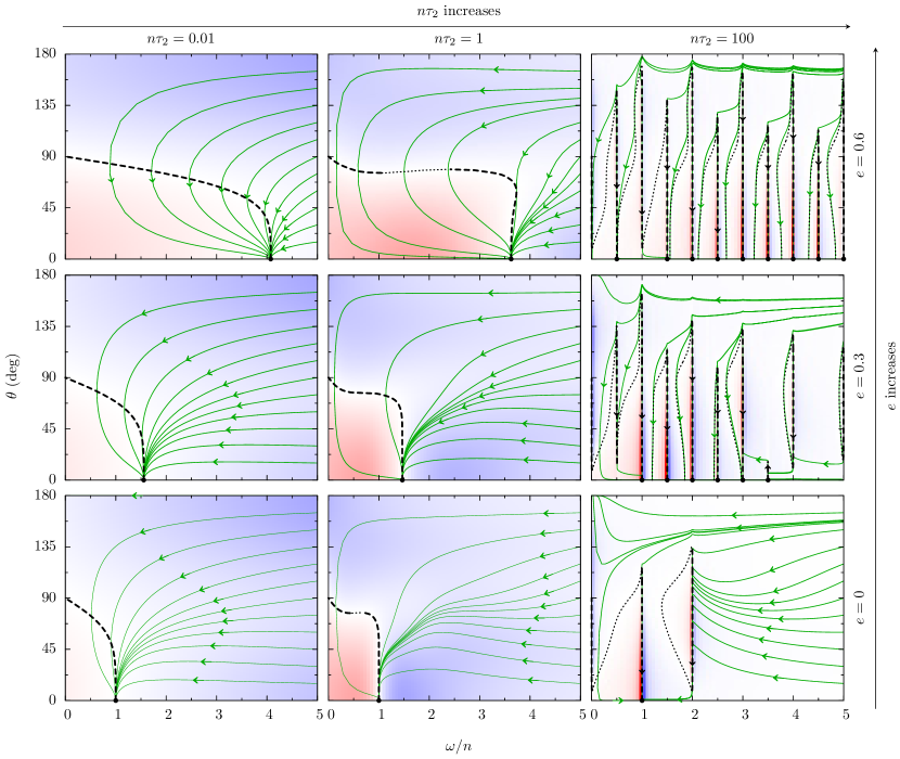
Figure 2: Secular trajectories of the spin-axis in the plane obliquity $\theta$ versus rotation $\omega/n$. From left to right, the product $n\tau_{2}$ increases from 0.01 to 100. From bottom to top, the eccentricity increases from 0.0 to 0.6. Trajectories of the spin-axis are represented by green solid curves, the background color represents the derivative of $\omega$: in blue $\omega$ decreases, in red $\omega$ increases. The locus of rotation equilibria such that $d\omega/dt=0$ (irregardless of $d\theta/dt$) are highlighted by black curves. Dashed ones and dotted ones represent stable and unstable equilibria, respectively. Black dots on the $x$-axis are the fixed points. This figure has been made by integration of Eqs. (25) with $t_{1}$, $t_{2}$, and $t_{3}$ taken from Tab. 1. Sums have been truncated at $|k|\leq 100$.

It should be noted that the trajectory of the spin in the plane $(\omega/n,\theta)$ only depends on the ratio $\omega/n$, the obliquity $\theta$, the eccentricity $e$, and the product $n\tau_{2}$. A few of them are plotted in Figure 2 for $e\in\{0,0.3,0.6\}$ and $n\tau_{2}\in\{0.01,1,100\}$. Plots are limited to positive $\omega/n$ but they can be extended to negative rotations with the symmetry $(\omega,\theta)\leftrightarrow(-\omega,\pi-\theta)\ .$ Indeed, these two pairs are equivalent although they do not correspond to the same physical state (Correia and Laskar, 2001).

For $n\tau_{2}=0.01$ (Fig. 2 left column), i.e. when the viscous timescale is much shorter than the orbital period, the system is in the linear regime. All trajectories converge smoothly towards a prograde pseudo-synchronous rotation on the $x$-axis. Evolutions are free from temporary captures in spin-orbit resonance.

At $n\tau_{2}=100$ (Fig. 2 right column), the viscous timescale is much greater than the orbital period. Resonant features appear in the phase space even at zero eccentricity. Indeed, when $e=0$, if the planet is tilted, its rotation can be trapped in three different spin-orbit resonances, namely the 0:1, the 1:1, and the 2:1. However, the obliquity is decreasing along these resonances and, in the planar configuration, only the synchronous holds. The final state is thus the synchronous rotation. At higher eccentricities, we observe many more spin-orbit equilibria for which $\omega/n$ is a half integer. As in the circular case, a few of these resonances disappear at zero obliquity but several do persist. The case $e=0.3$ shows an interesting feature: let us consider a trajectory (not represented) starting at $\omega/n=4.5$ and $\theta=90^{\circ}$. Because this point is in a blue region, $\omega$ decreases until the rotation reaches the 4:1 resonance. Then, the system follows the resonance downward until the obliquity reaches about $5^{\circ}$ where the resonance disappears. The subsequent evolution is horizontal toward the 7:2 resonance. But this resonance is special because $d\theta/dt>0$. Thus, the system climbs this resonance up to its end at $\theta\approx 16^{\circ}$. The field line continues on the left towards the 3:1 spin-orbit resonance. At last, this resonance has a “normal” behavior, the obliquity decreases and the system ends up in a planar state with $\omega/n=3$. This prediction has been tested numerically by integration of the instantaneous equations of motion (Eqs. 14) (see Section 6.3). At higher eccentricity ($e=0.6$), all spin-orbit resonances displayed in Fig. 2, i.e. with $\omega/n\leq 5$, are such that $d\theta/dt$ is negative. Thus, along these resonances the obliquity varies in a monotonous way toward the planar configuration. Note that if a system starts with a fast rotation $\omega\gg n$, it will almost certainly never reach an intermediate spin-orbit resonance such as the 2:1 or the 3:1 because the obliquity would have to be very fine tuned close around $164^{\circ}$ at $\omega/n=5$.

For $n\tau_{2}=1$ (Fig. 2 middle column), the evolution does not show any spin-orbit resonances. The phase space is qualitatively similar to that of the linear regime. Field lines are only slightly deformed.

6 Application to HD 80606 b

In this section, we apply the model at the quadrupole order $l_{\mathrm{max}}=2$ to HD 80606 b. The formalism is the same as in (Correia et al, 2014), except that only the planar case was studied in this previous work. Here, we extend the analysis to the spatial case by allowing non-zero initial obliquities. First, we briefly recall the results obtained for HD 80606 b in the planar case, with $\tau_{e}=0$ and $\tau_{2}$ ranging between $10^{-5}$ and $10^{0}$ yr. Then, we present our results in the spatial problem.

6.1 Description of the planar evolution

As shown by the differential equation (7), tides can be seen as a low-pass filter between the excitation $Z^{e}_{l,m}$ and the response $Z^{\nu}_{l,m}=Z_{l,m}$. If the cutoff frequency $1/\tau_{2}$ is much greater than the orbital frequency $n$, i.e., $\tau_{2}\ll 10^{-2}$ yr, all the “signal” is transmitted by the filter but with a small phase shift. This is equivalent to the constant time-lag model $\Delta t=\tau_{2}$. The surface of the planet undergoes strong deformations at the orbital frequency but the amount of dissipation is low because of the weak viscosity. Once the spin of the planet is damped, it follows a pseudo-synchronous equilibrium $\Omega_{e}$ which is a function of the eccentricity $e$. Here, we recall its expression in the spatial case, i.e. with obliquity $\theta$, in anticipation to the forthcoming section. We have (e.g., Correia et al, 2011)

$$\frac{\Omega_{e}}{n}=\frac{1+\frac{15}{2}e^{2}+\frac{45}{8}e^{4}+\frac{5}{16}e^{6}}{(1-e^{2})^{3/2}\left(1+3e^{2}+\frac{3}{8}e^{4}\right)}\frac{2\cos\theta}{1+\cos^{2}\theta}\ .$$ (26)

For $\tau_{2}\gg 10^{-2}$ yr, the cutoff frequency is less than the mean motion rate. The deformation of the planet, represented by

$$J_{2}=-Z_{2,0}\qquad\mathrm{and}\qquad\epsilon=\sqrt{C_{22}^{2}+S_{22}^{2}}=\sqrt{6}|Z_{22}|\ ,$$

only sees a mean excitation averaged over the mean anomaly and takes the expression (Correia et al, 2014)

$$\langle J_{2}\rangle_{M} =k^{0}_{2}\left(\frac{\Omega^{2}R^{3}}{3Gm_{1}}+\frac{1}{2}\frac{m_{0}}{m_{1}}\left(\frac{R}{a}\right)^{3}(1-e^{2})^{3/2}\right)\ ,$$ (27a)

$$\langle\epsilon_{p}\rangle_{M} =\frac{k^{0}_{2}}{4}\frac{m_{0}}{m_{1}}\left(\frac{R}{a}\right)^{3}X^{-3,2}_{2p}(e)\ ,$$ (27b)

with $p=[2\Omega/n]/2$, where $[x]$ means the nearest integer of $x$ ($[x]\in\mathbb{Z}$ and $[x]-1/2\leq x<[x]+1/2$). Thus, despite a high viscosity, dissipation is low because the deformation is weak and slow. In that case, the constant time-lag model does not hold anymore. The planet rotation gets trapped in spin-orbit resonances $\Omega/n=p$, the pseudo-synchronous state is not an equilibrium anymore.

At $\tau_{2}\approx 10^{-2}$ yr, the orbital frequency is of the same order of magnitude as the cutoff frequency. A few harmonics of the orbital period pass the filter and are retrieved in the deformation of the planet. Moreover, the viscosity is higher than in the constant-time lag regime. Both effects generate strong dissipation and a fast decay of the semi-major axis and eccentricity.

6.2 Fast damping of the obliquity and subsequent planar evolution

Numerical simulations were performed using the formalism in the inertial reference frame (Sect. 4, Eqs. 14). We have tested different values of $\tau_{2}$, but the main conclusion of this section remains unchanged. Thus, we only present results corresponding to the intermediate case $\tau_{2}=10^{-2}$ yr.

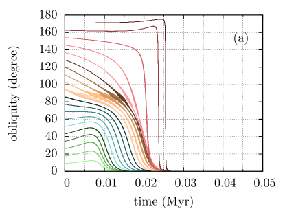
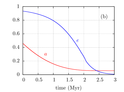
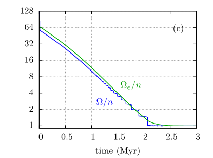
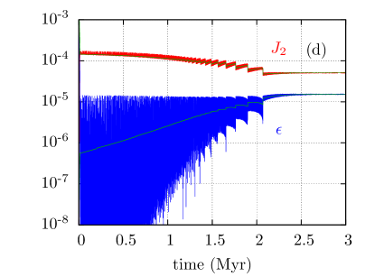
Figure 3: Time evolution of HD 80606 b for $\tau_{2}=10^{-2}$ yr ($0.21\leq n\tau_{2}\leq 0.95$). Panel (a) shows 400 evolutions with a grid of initial spin-axes (20 obliquities ranging between 0 and 180 degrees times 20 precession angles ranging between 0 and 360 degrees). The other three figures are initialized with an obliquity of 60 degrees and a precession angle of 0 degree. We plot the obliquity (a), the semi-major axis (in au) and the eccentricity (b), the ratio between the planet spin rate and the orbital mean motion (c), and the planet $J_{2}$ and $\epsilon$ (d). The green line gives the equilibrium rotation (Eq. 26) (c), and the equilibrium values for $J_{2}$ and $\epsilon$, respectively (Eqs. 27a and 27b) (d).

Figure 3a depicts the evolution of the planet obliquity for 400 different initial conditions: 20 obliquities regularly spread between 0 and 180 degrees times 20 precession angles equispaced over 360 degrees. The initial precession angle does not play a significant role in the evolution of the system. At a given initial obliquity, all integration’s closely follow the same track. This result strengthens the approximation made in the previous section where we averaged the secular equations of motion over the longitude of the pericenter $\varpi$. In comparison, obliquities starting at different values can have distinct initial slopes. But in all cases, the obliquity is fully damped before 30 kyr, a timescale much shorter than that of the orbital decay.

The subsequent evolution ($t>30$ kyr) is done at zero obliquity. The problem is thus fully described by the planar model. Indeed, we recover the results displayed in (Correia et al, 2014, Fig. 6). The semi-major axis and the eccentricity are damped within a timescale of 2 Myr (Fig. 3b), the spin rate of the planet follows a series of resonances with the orbital mean motion (Fig. 3c), and the deformation of the planet oscillates with intermediate amplitudes around its equilibrium given by Eqs. 27.

Numerical experiments performed with different values of $\tau_{2}$ are similar. Obliquities are fully damped in a timescale much shorter than those associated to the semi-major axis and the eccentricity. Once the system becomes planar, we retrieve the evolution observed in (Correia et al, 2014). This result reveals that the motion of the spin-axis can be followed independently from that of the orbit. Thus, we can directly compare the numerical solutions of the instantaneous equations of motion (Eqs. 14) to those dictated by the secular torque (Section 5).

6.3 Instantaneous versus secular evolution

In this section, we keep the system HD 80606 b as a proxy to analyze the spatial evolution of spin-axes given by the instantaneous equations of motion (Eqs. 14). To start a simulation at a given eccentricity $e$, we choose the semi-major axis $a$ as if the system had evolved from its current orbit ($e_{0}=0.933$ and $a_{0}=0.455$ au) with a constant angular momentum, i.e., such that $a(1-e^{2})=a_{0}(1-e_{0}^{2})$. In all simulations, we set the initial precession angle and the initial longitude of periapsis to zero.

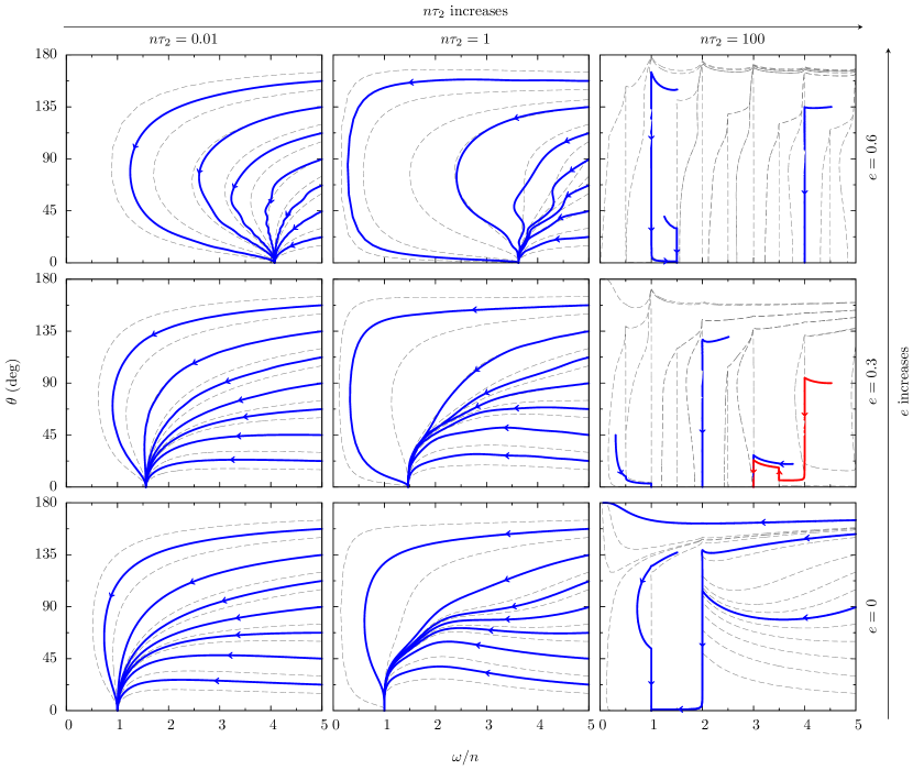
Figure 4: Instantaneous versus secular evolution. Solid thick curves are the trajectories obtained by integration of the instantaneous equations of motion (Eqs. 14). Thin dashed curves are the field lines of the Figure 2 obtained by integration of the secular equations of motion (Eqs. 25). The red curve is the trajectory discussed in Section 5.5.

Figure 4 displays the results in the plane $(\omega/n,\theta)$ as in Figure 2 together with the secular field lines obtained in Section 5. The match between the two approaches is excellent. Solutions of the instantaneous equations of motion (Eqs. 14) closely follow the paths dictated by the secular torque (Eqs. 25), except however for $e=0.6$ and $n\tau_{2}=1$ where the instantaneous evolutions exhibit more wiggles than the secular ones. In particular, we retrieve the special trajectory at $e=0.3$ and $n\tau_{2}=100$ discussed in Section 5.5 which starts at $\omega/n=4.5$ and $\theta=90^{\circ}$ (plotted in red in Figure 4). The time evolution of this trajectory is shown in Figure 5. We see that the system spends most of the time in spin-orbit resonant configurations. The temporal evolution also emphasizes the peculiar behavior of the 7:2 resonance in which the planet obliquity increases.

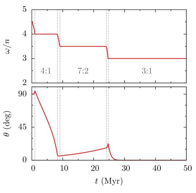
Figure 5: Time evolution of HD 80606 b with the same initial conditions as the red trajectory in Figure 4 ($e=0.3$ and $n\tau_{2}=100$). Vertical dashed lines delimit regions of spin-orbit resonance. Note that after 50 Myr, the eccentricity and the semi-major axis have only decreased by about $3\times 10^{-4}$ and $10^{-3}$ in relative value, respectively. They can thus be considered constant as in Figure 4.

7 Conclusion

In this paper, we present a tidal theory based on the Maxwell rheology valid in the spatial case. This extends the models presented by Ferraz-Mello (2013) and Correia et al (2014) which were restricted to planar configurations.

The evolution of the deformation of the planet, given by a first order differential equation (Eqs. 9d and 14d), is integrated numerically together with the orbital motion. As already noted by Correia et al (2014), this way allows to compute the instantaneous variation of the shape of the planet for all perturbations, even for non-periodic ones. There is no need to decompose the excitation in an infinite Fourier series as in, e.g., Kaula (1964). By consequence, the formalism is regular at all eccentricities, spin rates, and obliquities.

For this problem, we have chosen a formalism taken from quantum theory, conceived for angular momentum representations, and based on complex spherical harmonics $Y_{l,m}$. Our choice has been motivated by the following reasons: the gravitational potential of the planet is easily expanded in $Y_{l,m}$; $Y_{l,m}$’s can be conveniently expressed in terms of Cartesian coordinates; tidal force and torque have compact expressions because $Y_{l,m}$’s are the eigenvectors of the ladder operators $\vec{\nabla}$ and $\vec{J}=-\mathrm{i}\vec{x}\times\vec{\nabla}$; our model is given at any multipole order thanks to the recurrence relations present in many quantum mechanics textbooks such as (Varshalovich et al, 1988).

Tidal equations are naturally written in the frame of the body, but this choice is not convenient for the analysis of the orbital evolution. Here, we provide the equations of motion both in the body frame ${\cal F}_{p}$ (Eqs. 9) and in the inertial frame ${\cal F}_{0}$ (Eqs. 14). If the planet does not have any permanent zonal coefficients, the description of the problem in ${\cal F}_{0}$ presents a numerical advantage. Indeed, whatever is the rotation speed of the planet, the tidal bulge follows the perturbing body. Thus, the integration time step can be adjusted to the orbital motion even if the planet rotates much faster.

The equations of motion written in the inertial frame allowed us to compute the secular tidal torque as a Fourier series averaged over the orbital revolution and over the precession period. We provide an explicit vectorial expression of this torque at the quadrupolar order as well as the general expression at any multipole order. Maps of the secular evolution of the spin-axis show many resonant features when the viscous timescale is longer than the orbital period. This characteristic was already present in planar studies but here we observe that non-synchronous spin-orbit resonances appear in the spatial case even at zero eccentricity. In most of these resonant states, the obliquity decreases to zero, but we found a peculiar situation were the obliquity is instead growing.

We applied our model to HD 80606 with different values of relaxation time and different initial obliquities. We observed that in all cases, the obliquity is damped faster than the semi-major axis and the eccentricity. Once the system becomes planar, the evolution follows the path described in (Correia et al, 2014). In particular, when the relaxation time is greater than the orbital period, the planet gets trapped in successive spin-orbit resonances even though it does not have any permanent multipole (Correia et al, 2014). We have also analyzed in more detail the evolution of the spin-axis during the phase where the obliquity is not fully damped. Results are in good agreement with the predictions made with the averaged equations. We nevertheless observe wiggles at high eccentricity which were not present in the secular phase-space.

Our model can also be applied to close-in super-Earths for which the relaxation time of the mantle is almost certainly longer than the orbital period. As these planets are often found with planetary companions, their eccentricities are never exactly zero (e.g., Laskar et al, 2012). This implies that short-period terrestrial exoplanets are likely in spin-orbit resonances (Correia et al, 2014). In addition, as in the solar system, they also present small mutual inclinations of about $1^{\circ}$ on average (Tremaine and Dong, 2012; Figueira et al, 2012; Fabrycky et al, 2014). This value is large enough to perturb the long-term evolution of their obliquity and, even if the orbit is circular, a forced obliquity can trap the rotation in a non-synchronous spin-orbit resonance state. Our formalism is thus well adapted to model the evolution of these planets spin-axis and to infer constraints on their habitability. We also envision to extend the formalism to thermal atmospheric tides which have the same frequency dependence as Maxwell rheology (Auclair-Desrotour et al, 2016).

Appendix A Spherical harmonic

By convention, Legendre associated polynomials are defined as

$$P_{l,m}(x)=\frac{1}{2^{l}l!}(1-x^{2})^{m/2}\frac{d^{l+m}}{dx^{l+m}}(x^{2}-1)^{l}\ ,$$ (28)

with the symmetry

$$P_{l,-m}(x)=(-1)^{m}\frac{(l-m)!}{(l+m)!}P_{l,m}(x)\ .$$ (29)

The Schmidt semi-normalized spherical harmonics are defined as

$$Y_{l,m}(\theta,\phi)=(-1)^{m}\sqrt{\frac{(l-m)!}{(l+m)!}}P_{l,m}(\cos\theta)\mathrm{e}^{\mathrm{i}m\phi}$$ (30)

with the symmetry

$$Y_{l,-m}(\theta,\phi)=(-1)^{m}\bar{Y}_{l,m}(\theta,\phi)\ .$$ (31)

Using the complex Cartesian coordinate system as defined in (Varshalovich et al, 1988), for any unit vector $\hat{x}$, we have

$$Y_{0,0}(\hat{\vec{x}}) =1\ ,$$ (32a)

$$Y_{1,0}(\hat{\vec{x}}) =\hat{x}_{0}\ ,$$ (32b)

$$Y_{1,1}(\hat{\vec{x}}) =\hat{x}_{+}\ ,$$ (32c)

$$l\,Y_{l,0}(\hat{\vec{x}}) =(2l-1)\hat{x}_{0}Y_{l-1,0}(\hat{\vec{x}})-(l-1)Y_{l-2,0}(\hat{\vec{x}})\ ,$$ (32d)

$$\sqrt{l+m}Y_{l,m}(\hat{\vec{x}}) =\sqrt{l-m}\,\hat{x}_{0}Y_{l-1,m}(\hat{\vec{x}})+\sqrt{2(l+m-1)}\hat{x}_{+}Y_{l-1,m-1}\ .$$ (32e)

The last two equations (32d and 32e) allow to recursively compute all spherical harmonics of order $m\geq 0$. Those with $m<0$ are deduced from the symmetry relation (31). Up to the degree 3 included, we have

$$\left\{\begin{array}[]{ll}Y_{2,0}&=\displaystyle\frac{1}{2}(3\hat{x}_{0}^{2}-1)\\[10.00002pt] Y_{2,1}&=\displaystyle\sqrt{3}\hat{x}_{0}\hat{x}_{+}\\[10.00002pt] Y_{2,2}&=\displaystyle\frac{\sqrt{6}}{2}\hat{x}_{+}^{2}\end{array}\right.\ ,\qquad\left\{\begin{array}[]{ll}Y_{3,0}&=\displaystyle\frac{5}{2}\hat{x}_{0}^{3}-\frac{3}{2}\hat{x}_{0}\\[10.00002pt] Y_{3,1}&=\displaystyle\frac{\sqrt{6}}{4}\left(5\hat{x}_{0}^{2}\hat{x}_{+}-\hat{x}_{+}\right)\\[10.00002pt] Y_{3,2}&=\displaystyle\frac{\sqrt{30}}{2}\hat{x}_{0}\hat{x}_{+}^{2}\\[10.00002pt] Y_{3,3}&=\displaystyle\frac{\sqrt{10}}{2}\hat{x}_{+}^{3}\end{array}\right.\ .$$ (33)

Appendix B Ladder operators

Regular solid harmonics $x^{l}Y_{l,m}(\hat{\vec{x}})$ and irregular ones $Y_{l,m}(\hat{\vec{x}})/x^{l+1}$ are eigenvectors of each component of the gradient operator $\vec{\nabla}=(\nabla_{+},\nabla_{0},\nabla_{-})$ and of the angular momentum operator $\vec{J}=(J_{+},J_{0},J_{-})$. The respective eigenvalues can be found in (e.g., Varshalovich et al, 1988). We have

$$\nabla_{+}\left(x^{l}Y_{l,m}(\hat{\vec{x}})\right) =-\sqrt{\frac{(l-m-1)(l-m)}{2}}\,x^{l-1}Y_{l-1,m+1}(\hat{\vec{x}})$$

$$\nabla_{0}\left(x^{l}Y_{l,m}(\hat{\vec{x}})\right) =+\sqrt{(l+m)(l-m)}\,x^{l-1}Y_{l-1,m}(\hat{\vec{x}})$$ (34)

$$\nabla_{-}\left(x^{l}Y_{l,m}(\hat{\vec{x}})\right) =-\sqrt{\frac{(l+m-1)(l+m)}{2}}\,x^{l-1}Y_{l-1,m-1}(\hat{\vec{x}})\ ,$$

$$\nabla_{+}\left(\frac{1}{x^{l+1}}Y_{l,m}(\hat{\vec{x}})\right) =-\sqrt{\frac{(l+m+1)(l+m+2)}{2}}\frac{1}{x^{l+2}}Y_{l+1,m+1}(\hat{\vec{x}})$$

$$\nabla_{0}\left(\frac{1}{x^{l+1}}Y_{l,m}(\hat{\vec{x}})\right) =-\sqrt{(l+m+1)(l-m+1)}\frac{1}{x^{l+2}}Y_{l+1,m}(\hat{\vec{x}})$$ (35)

$$\nabla_{-}\left(\frac{1}{x^{l+1}}Y_{l,m}(\hat{\vec{x}})\right) =-\sqrt{\frac{(l-m+1)(l-m+2)}{2}}\frac{1}{x^{l+2}}Y_{l+1,m-1}(\hat{\vec{x}})\ ,$$

and

$$J_{+}\bigg{(}f(x)Y_{l,m}(\hat{\vec{x}})\bigg{)} =-\sqrt{\frac{l(l+1)-m(m+1)}{2}}f(x)Y_{l,m+1}(\hat{\vec{x}})$$

$$J_{0}\bigg{(}f(x)Y_{l,m}(\hat{\vec{x}})\bigg{)} =mf(x)Y_{l,m}(\hat{\vec{x}})$$ (36)

$$J_{-}\bigg{(}f(x)Y_{l,m}(\hat{\vec{x}})\bigg{)} =+\sqrt{\frac{l(l+1)-m(m-1)}{2}}f(x)Y_{l,m-1}(\hat{\vec{x}})\ ,$$

where $f(x)$ is any function of the modulus $x=\|\stackrel{{\scriptstyle\text{\raisebox{-4.0pt}[1.0pt][0.0pt]{$\mathchar 382\relax$}}}}{{x}}\|$.

Appendix C Rotation and Wigner matrices

Let a vector $\stackrel{{\scriptstyle\text{\raisebox{-4.0pt}[1.0pt][0.0pt]{$\mathchar 382\relax$}}}}{{x}}$ and two coordinate systems ${\cal B}$ and ${\cal B}^{\prime}$ such that $\vec{x}$ and $\vec{x}^{\prime}$ are the coordinates of $\stackrel{{\scriptstyle\text{\raisebox{-4.0pt}[1.0pt][0.0pt]{$\mathchar 382\relax$}}}}{{x}}$ in ${\cal B}$ and ${\cal B}^{\prime}$, respectively. Let us further assume that $\vec{x}$ and $\vec{x}^{\prime}$ are related to each other by a rotation of the form

$$\vec{x}={\mathsf{R}}_{3}(\alpha){\mathsf{R}}_{2}(\beta){\mathsf{R}}_{3}(\gamma)\vec{x}^{\prime}\ ,$$

where ${\mathsf{R}}_{3}$ and ${\mathsf{R}}_{2}$ are the matrices of rotation around the third and the second axes, respectively. Wigner D matrix $\mathsf{D}^{l}_{m,m^{\prime}}(\alpha,\beta,\gamma)$ is defined such that (e.g., Varshalovich et al, 1988)

$$Y_{l,m}(\hat{\vec{x}}^{\prime})=\sum_{m^{\prime}=-l}^{l}\mathsf{D}^{l}_{m^{\prime},m}(\alpha,\beta,\gamma)Y_{l,m^{\prime}}(\hat{\vec{x}})\ .$$ (37)

Each element $\mathsf{D}^{l}_{m,m^{\prime}}(\alpha,\beta,\gamma)$ can be written as (e.g., Varshalovich et al, 1988)

$$\mathsf{D}^{l}_{m,m^{\prime}}(\alpha,\beta,\gamma)=\mathrm{e}^{-\mathrm{i}m\alpha}\mathsf{d}^{l}_{m,m^{\prime}}(\beta)\mathrm{e}^{-\mathrm{i}m^{\prime}\gamma}\ ,$$ (38)

where $\mathsf{d}^{l}_{m,m^{\prime}}(\beta)$ is the Wigner d matrix. The inverse $\mathsf{D}^{l}_{m,m^{\prime}}(-\gamma,-\beta,-\alpha)$ is given by the adjoint $\bar{\mathsf{D}}^{l}_{m^{\prime},m}(\alpha,\beta,\gamma)$ of $\mathsf{D}^{l}_{m,m^{\prime}}(\alpha,\beta,\gamma)$:

$$\mathsf{D}^{l}_{m,m^{\prime}}(-\gamma,-\beta,-\alpha)=\mathrm{e}^{\mathrm{i}m^{\prime}\alpha}\mathsf{d}^{l}_{m^{\prime},m}(\beta)\mathrm{e}^{\mathrm{i}m\gamma}\ .$$

The convention 3-2-3 of the rotation (Eq. 37) is such that $\mathsf{d}^{l}_{m,m^{\prime}}(\beta)$ is a real function. Wigner d matrix possesses many symmetries, among which (e.g., Varshalovich et al, 1988)

$$\mathsf{d}^{l}_{m,m^{\prime}}(\beta)=(-1)^{m-m^{\prime}}\mathsf{d}^{l}_{-m,-m^{\prime}}(\beta)=(-1)^{m-m^{\prime}}\mathsf{d}^{l}_{m^{\prime},m}(\beta)=\mathsf{d}^{l}_{-m^{\prime},-m}(\beta)\ .$$

Wigner d matrix can be constructed recursively using the hereinabove symmetries, the following initialization (e.g., Varshalovich et al, 1988)

$$\mathsf{d}^{0}_{0,0}(\beta)=1\,,\ \mathsf{d}^{1}_{0,0}(\beta)=\cos\beta\,,\ \mathsf{d}^{1}_{1,-1}(\beta)=\frac{1-\cos\beta}{2}\,,\ \mathsf{d}^{1}_{1,0}(\beta)=-\frac{\sin\beta}{\sqrt{2}}\,,\ \mathsf{d}^{1}_{1,1}(\beta)=\frac{1+\cos\beta}{2}$$ (39)

and the recurrence relation (Gimbutas and Greengard, 2009)

$$\begin{split}\mathsf{d}^{l}_{m,m^{\prime}}(\beta)=&+\sqrt{\frac{(l+m^{\prime})(l+m^{\prime}-1)}{(l+m)(l+m-1)}}\mathsf{d}^{1}_{1,1}(\beta)\mathsf{d}^{l-1}_{m-1,m^{\prime}-1}(\beta)\\ &-\sqrt{\frac{(l+m^{\prime})(l-m^{\prime})}{(l+m)(l+m-1)}}\sin(\beta)\mathsf{d}^{l-1}_{m-1,m^{\prime}}(\beta)\\ &+\sqrt{\frac{(l-m^{\prime})(l-m^{\prime}-1)}{(l+m)(l+m-1)}}\mathsf{d}^{1}_{1,-1}(\beta)\mathsf{d}^{l-1}_{m-1,m^{\prime}+1}(\beta)\end{split}$$ (40)

which also implies

$$\mathsf{d}^{l}_{l,l}(\beta)=\mathsf{d}^{1}_{1,1}(\beta)\mathsf{d}^{l-1}_{l-1,l-1}(\beta)\qquad\text{and}\qquad\mathsf{d}^{l}_{l,-l}(\beta)=\mathsf{d}^{1}_{1,-1}(\beta)\mathsf{d}^{l-1}_{l-1,1-l}(\beta)\ .$$ (41)

The algorithm is the following:

Algorithm 1 Calculate Wigner d matrix

  initialize $\mathsf{d}^{1}_{0,0}$, $\mathsf{d}^{1}_{1,1}$, $\mathsf{d}^{1}_{1,0}$, and $\mathsf{d}^{1}_{1,-1}$ from (Eq. 39)

  calculate the other terms of order $1$ using the symmetries (Eq. 38)

  for $l=2$ to $l_{\mathrm{max}}$ do

     // apply the recurrence relations as follows

     for $m=0$ to $l$ do

        for $m^{\prime}=\operatorname{MAX}(-m,1-l)$ to $\operatorname{MIN}(m,l-1)$ do

           calculate $\mathsf{d}^{l}_{m,m^{\prime}}$ using (Eq. 40)

        end for

     end for

     compute $\mathsf{d}^{l}_{l,l}$ and $\mathsf{d}^{l}_{l,-l}$ from (Eq. 41)

     calculate the other terms of order $l$ using the symmetries (Eq. 38)

  end for

For completeness, we also provide the explicit terms at order $l=2$ in Table 2.

Table 2: Explicit Wigner d matrix $\mathsf{d}^{2}_{m,m^{\prime}}(\beta)$

	2	1	0	-1	-2
2	$\displaystyle\frac{(1+\cos\beta)^{2}}{4}$	$\displaystyle-\frac{\sin\beta(1+\cos\beta)}{2}$	$\displaystyle\frac{1}{2}\sqrt{\frac{3}{2}}\sin^{2}\beta$	$\displaystyle-\frac{\sin\beta(1-\cos\beta)}{2}$	$\displaystyle\frac{(1-\cos\beta)^{2}}{4}$
1	$\displaystyle\frac{\sin\beta(1+\cos\beta)}{2}$	$\displaystyle\frac{2\cos^{2}\beta+\cos\beta-1}{2}$	$\displaystyle-\sqrt{\frac{3}{2}}\sin\beta\cos\beta$	$\displaystyle-\frac{2\cos^{2}\beta-\cos\beta-1}{2}$	$\displaystyle-\frac{\sin\beta(1-\cos\beta)}{2}$
0	$\displaystyle\frac{1}{2}\sqrt{\frac{3}{2}}\sin^{2}\beta$	$\displaystyle\sqrt{\frac{3}{2}}\sin\beta\cos\beta$	$\displaystyle\frac{3\cos^{2}\beta-1}{2}$	$\displaystyle-\sqrt{\frac{3}{2}}\sin\beta\cos\beta$	$\displaystyle\frac{1}{2}\sqrt{\frac{3}{2}}\sin^{2}\beta$
-1	$\displaystyle\frac{\sin\beta(1-\cos\beta)}{2}$	$\displaystyle-\frac{2\cos^{2}\beta-\cos\beta-1}{2}$	$\displaystyle\sqrt{\frac{3}{2}}\sin\beta\cos\beta$	$\displaystyle\frac{2\cos^{2}\beta+\cos\beta-1}{2}$	$\displaystyle-\frac{\sin\beta(1+\cos\beta)}{2}$
-2	$\displaystyle\frac{(1-\cos\beta)^{2}}{4}$	$\displaystyle\frac{\sin\beta(1-\cos\beta)}{2}$	$\displaystyle\frac{1}{2}\sqrt{\frac{3}{2}}\sin^{2}\beta$	$\displaystyle\frac{\sin\beta(1+\cos\beta)}{2}$	$\displaystyle\frac{(1+\cos\beta)^{2}}{4}$

Appendix D Time derivatives

Let a function $f(\stackrel{{\scriptstyle\text{\raisebox{-4.0pt}[1.0pt][0.0pt]{$\mathchar 382\relax$}}}}{{x}},t)$ developed in spherical harmonics as

$$f(\stackrel{{\scriptstyle\text{\raisebox{-4.0pt}[1.0pt][0.0pt]{$\mathchar 382\relax$}}}}{{x}},t)=\sum_{l,m}\bar{z}_{l,m}(t)Y_{l,m}(\hat{\vec{x}})$$ (42)

in the inertial frame ${\cal F}_{0}$, and as

$$f(\stackrel{{\scriptstyle\text{\raisebox{-4.0pt}[1.0pt][0.0pt]{$\mathchar 382\relax$}}}}{{x}},t)=\sum_{l,m}\bar{Z}_{l,m}(t)Y_{l,m}(\hat{\vec{X}})$$ (43)

in the body frame ${\cal F}_{p}$. For any constant vector $\stackrel{{\scriptstyle\text{\raisebox{-4.0pt}[1.0pt][0.0pt]{$\mathchar 382\relax$}}}}{{x}}$ in ${\cal F}_{p}$, we have

$$\dot{\vec{x}}=\vec{\omega}\times\vec{x}\qquad\mathrm{and}\qquad\dot{\vec{X}}=\vec{0}\ ,$$ (44)

with respect to the frame ${\cal F}_{p}$. By consequence, in ${\cal F}_{p}$, on the one hand,

$$\dot{f}(\stackrel{{\scriptstyle\text{\raisebox{-4.0pt}[1.0pt][0.0pt]{$\mathchar 382\relax$}}}}{{x}},t)=\sum_{l,m}\left(\dot{\bar{z}}_{l,m}(t)Y_{l,m}(\hat{\vec{x}})+\bar{z}_{l,m}(t)\dot{\vec{x}}\cdot\vec{\nabla}Y_{l,m}(\hat{\vec{x}})\right)\ ,$$ (45)

and on the other hand,

$$\dot{f}(\stackrel{{\scriptstyle\text{\raisebox{-4.0pt}[1.0pt][0.0pt]{$\mathchar 382\relax$}}}}{{x}},t)=\sum_{l,m}\dot{\bar{Z}}_{l,m}(t)Y_{l,m}(\hat{\vec{X}})\ .$$ (46)

But given that the time derivative of $\vec{x}$ is $\dot{\vec{x}}=\vec{\omega}\times\vec{x}$, we get

$$\dot{\vec{x}}\cdot\vec{\nabla}=(\vec{\omega}\times\vec{x})\cdot\vec{\nabla}=\mathrm{i}(\vec{\omega}\cdot\vec{J})$$ (47)

where $\vec{J}=-\mathrm{i}\vec{x}\times\vec{\nabla}$ is the angular momentum operator and where, by construction of the scalar product (Varshalovich et al, 1988),

$$\vec{\omega}\cdot\vec{J}=-\omega_{+}J_{-}+\omega_{0}J_{0}-\omega_{-}J_{+}\ .$$ (48)

We then define a matrix $\mathsf{J}(\vec{\omega})$ of size $(2l+1)\times(2l+1)$ such that

$$(\vec{\omega}\cdot\vec{J})Y_{l,m}(\hat{\vec{x}})=\sum_{m^{\prime}=-l}^{l}[\mathsf{J}(\vec{\omega})]^{l}_{m^{\prime},m}Y_{l,m^{\prime}}(\hat{\vec{x}})\ ,$$ (49)

where all non-zero coefficients are

$$\begin{array}[]{lll}\left[\mathsf{J}(\vec{\omega})\right]^{l}_{m-1,m}&=&-\sqrt{\frac{l(l+1)-m(m-1)}{2}}\omega_{+}\ ,\\ \left[\mathsf{J}(\vec{\omega})\right]^{l}_{m,m}&=&m\,\omega_{0}\ ,\\ \left[\mathsf{J}(\vec{\omega})\right]^{l}_{m+1,m}&=&+\sqrt{\frac{l(l+1)-m(m+1)}{2}}\omega_{-}\ .\end{array}$$ (50)

Combining Eqs. (10), (45-47), and (49), we obtain

$$\sum_{m^{\prime}}\mathsf{D}^{l}_{m,m^{\prime}}\dot{\bar{Z}}_{l,m^{\prime}}=\dot{\bar{z}}_{l,m}+\mathrm{i}\sum_{m^{\prime}}\,[\mathsf{J}(\vec{\omega})]^{l}_{m,m^{\prime}}{\bar{z}}_{l,m^{\prime}}\ .$$ (51)

Appendix E Fourier transform

Let two functions $f(\stackrel{{\scriptstyle\text{\raisebox{-4.0pt}[1.0pt][0.0pt]{$\mathchar 382\relax$}}}}{{x}},t)$ and $g(\stackrel{{\scriptstyle\text{\raisebox{-4.0pt}[1.0pt][0.0pt]{$\mathchar 382\relax$}}}}{{x}},t)$ expanded in spherical harmonics as $f=\sum_{l}f_{l}$ and $g=\sum_{l}g_{l}$ with

$$f_{l}(\stackrel{{\scriptstyle\text{\raisebox{-4.0pt}[1.0pt][0.0pt]{$\mathchar 382\relax$}}}}{{x}},t)=\sum_{m=-l}^{l}\bar{Z}_{l,m}(t)Y_{l,m}(\hat{\vec{X}})\qquad\text{and}\qquad g_{l}(\stackrel{{\scriptstyle\text{\raisebox{-4.0pt}[1.0pt][0.0pt]{$\mathchar 382\relax$}}}}{{x}},t)=\sum_{m=-l}^{l}\bar{Z}^{\prime}_{l,m}(t)Y_{l,m}(\hat{\vec{X}})$$

in the frame ${\cal F}_{p}$ and

$$f_{l}(\stackrel{{\scriptstyle\text{\raisebox{-4.0pt}[1.0pt][0.0pt]{$\mathchar 382\relax$}}}}{{x}},t)=\sum_{m=-l}^{l}\bar{z}_{l,m}(t)Y_{l,m}(\hat{\vec{x}})\qquad\text{and}\qquad g_{l}(\stackrel{{\scriptstyle\text{\raisebox{-4.0pt}[1.0pt][0.0pt]{$\mathchar 382\relax$}}}}{{x}},t)=\sum_{m=-l}^{l}\bar{z}^{\prime}_{l,m}(t)Y_{l,m}(\hat{\vec{x}})$$

in ${\cal F}_{0}$. Let $\alpha$, $\beta$, and $\gamma=\omega t$ be the three angles such that

$$\vec{x}=\mathsf{R}_{3}(\alpha)\mathsf{R}_{2}(\beta)\mathsf{R}_{3}(\gamma)\vec{X}\ .$$

We have then

$$z_{l,m}(t)=\sum_{m^{\prime}=-l}^{l}\bar{\mathsf{D}}^{l}_{m,m^{\prime}}(t)Z_{l,m^{\prime}}(t)\qquad\text{and}\qquad z^{\prime}_{l,m}(t)=\sum_{m^{\prime}=-l}^{l}\bar{\mathsf{D}}^{l}_{m,m^{\prime}}(t)Z^{\prime}_{l,m^{\prime}}(t)$$ (52)

with

$$\mathsf{D}^{l}_{m,m^{\prime}}(t)=\mathsf{D}^{l}_{m,m^{\prime}}(0)\mathrm{e}^{-\mathrm{i}m^{\prime}\omega t}\ .$$

Let us further assume that the two functions are related to each other in ${\cal F}_{p}$ by

$$f_{l}(\stackrel{{\scriptstyle\text{\raisebox{-4.0pt}[1.0pt][0.0pt]{$\mathchar 382\relax$}}}}{{x}},t)=h_{l}(t)*g_{l}(\stackrel{{\scriptstyle\text{\raisebox{-4.0pt}[1.0pt][0.0pt]{$\mathchar 382\relax$}}}}{{x}},t)\qquad\text{for all $l$}\ ,$$

where $h_{l}(t)\in\mathbb{R}$ is a real distribution. The symbol $*$ denotes the convolution product. As the convolution is done with respect to time, the orthogonality of the spherical harmonics implies that for all $l$ and $m$,

$$Z_{l,m}(t)=h_{l}(t)*Z^{\prime}_{l,m}(t)\ .$$ (53)

Combining Eqs. (52) and (53), we get

$$z_{l,m}(t) =\sum_{m^{\prime}=-l}^{l}\sum_{m"=-l}^{l}\int_{-\infty}^{\infty}\bar{\mathsf{D}}^{l}_{m,m^{\prime}}(t)h_{l}(t-t^{\prime}){\mathsf{D}}^{l}_{m",m^{\prime}}(t^{\prime})z^{\prime}_{l,m"}(t^{\prime})\,dt^{\prime}$$

$$=\sum_{m"=-l}^{l}\mathsf{h}^{l}_{m,m"}(t)*z^{\prime}_{l,m"}(t)\ ,$$ (54)

where

$$\mathsf{h}^{l}_{m,m"}(t)=\sum_{m^{\prime}=-l}^{l}\bar{\mathsf{D}}^{l}_{m,m^{\prime}}(0)h_{l}(t)\mathrm{e}^{\mathrm{i}m^{\prime}\omega t}\mathsf{D}^{l}_{m",m^{\prime}}(0)\ .$$

In particular, if the rotation axis $\stackrel{{\scriptstyle\text{\raisebox{-4.0pt}[1.0pt][0.0pt]{$\mathchar 382\relax$}}}}{{\omega}}$ is aligned with the third axis of ${\cal F}_{0}$ and ${\cal F}_{p}$, i.e., if $\alpha=\beta=0$, $\mathsf{h}^{l}_{m,m"}(t)$ is diagonal and we obtain

$$z_{l,m}(t)=\left(h_{l}(t)\mathrm{e}^{\mathrm{i}m\omega t}\right)*z^{\prime}_{l,m}(t)\qquad\text{if\quad$\alpha=\beta=0$}\ .$$ (55)

Taking the Fourier transform of Eqs. (54) and (55), we get

$$\text{\@text@baccent{$z$}}_{l,m}(\nu)=\sum_{m"=-l}^{l}\text{\@text@baccent{$\tens h$}}^{l}_{m,m"}(\nu)\text{\@text@baccent{$z$}}^{\prime}_{l,m"}(\nu)\quad\text{with}\quad\text{\@text@baccent{$\tens h$}}^{l}_{m,m"}(\nu)=\sum_{m^{\prime}=-l}^{l}\bar{\mathsf{D}}^{l}_{m,m^{\prime}}(0)\text{\@text@baccent{$h$}}_{l}(\nu-m^{\prime}\omega)\mathsf{D}^{l}_{m",m^{\prime}}(0)\ ,$$

on the one hand, and

$$\text{\@text@baccent{$z$}}_{l,m}(\nu)=\text{\@text@baccent{$h$}}_{l}(\nu-m\omega)\text{\@text@baccent{$z$}}^{\prime}_{l,m}(\nu)\qquad\text{if\quad$\alpha=\beta=0$}\ ,$$

on the other.

References

• Auclair-Desrotour et al (2016) Auclair-Desrotour P, Laskar J, Mathis S (2016) Atmospheric tides in Earth-Like planets. Astron. Astrophys. submitted
• Correia and Laskar (2001) Correia ACM, Laskar J (2001) The four final rotation states of Venus. Nature 411:767–770, DOI 10.1038/35081000
• Correia et al (2003) Correia ACM, Laskar J, de Surgy ON (2003) Long-term evolution of the spin of Venus. I. theory. Icarus 163:1–23, DOI 10.1016/S0019-1035(03)00042-3
• Correia et al (2011) Correia ACM, Laskar J, Farago F, Boué G (2011) Tidal evolution of hierarchical and inclined systems. Celestial Mechanics and Dynamical Astronomy 111:105–130, DOI 10.1007/s10569-011-9368-9, 1107.0736
• Correia et al (2014) Correia ACM, Boué G, Laskar J, Rodríguez A (2014) Deformation and tidal evolution of close-in planets and satellites using a Maxwell viscoelastic rheology. Astron. Astrophys. 571:A50, DOI 10.1051/0004-6361/201424211, 1411.1860
• Cunha et al (2015) Cunha D, Correia ACM, Laskar J (2015) Spin evolution of Earth-sized exoplanets, including atmospheric tides and core-mantle friction. International Journal of Astrobiology 14:233–254, DOI 10.1017/S1473550414000226, 1406.4544
• Darwin (1880) Darwin GH (1880) On the Secular Changes in the Elements of the Orbit of a Satellite Revolving about a Tidally Distorted Planet. Philosophical Transactions of the Royal Society of London 171:713–891
• Efroimsky (2012a) Efroimsky M (2012a) Bodily tides near spin-orbit resonances. Celestial Mechanics and Dynamical Astronomy 112:283–330, DOI 10.1007/s10569-011-9397-4, 1105.6086
• Efroimsky (2012b) Efroimsky M (2012b) Tidal Dissipation Compared to Seismic Dissipation: In Small Bodies, Earths, and Super-Earths. Astrophys. J. 746:150, DOI 10.1088/0004-637X/746/2/150, 1105.3936
• Efroimsky and Lainey (2007) Efroimsky M, Lainey V (2007) Physics of bodily tides in terrestrial planets and the appropriate scales of dynamical evolution. Journal of Geophysical Research (Planets) 112(E11):E12003, DOI 10.1029/2007JE002908, 0709.1995
• Efroimsky and Makarov (2013) Efroimsky M, Makarov VV (2013) Tidal Friction and Tidal Lagging. Applicability Limitations of a Popular Formula for the Tidal Torque. Astrophys. J. 764:26, DOI 10.1088/0004-637X/764/1/26, 1209.1615
• Fabrycky et al (2014) Fabrycky DC, Lissauer JJ, Ragozzine D, Rowe JF, Steffen JH, Agol E, Barclay T, Batalha N, Borucki W, Ciardi DR, Ford EB, Gautier TN, Geary JC, Holman MJ, Jenkins JM, Li J, Morehead RC, Morris RL, Shporer A, Smith JC, Still M, Van Cleve J (2014) Architecture of Kepler’s Multi-transiting Systems. II. New Investigations with Twice as Many Candidates. Astrophys. J. 790:146, DOI 10.1088/0004-637X/790/2/146, 1202.6328
• Ferraz-Mello (2013) Ferraz-Mello S (2013) Tidal synchronization of close-in satellites and exoplanets. A rheophysical approach. Celestial Mechanics and Dynamical Astronomy 116:109–140, DOI 10.1007/s10569-013-9482-y, 1204.3957
• Ferraz-Mello (2015) Ferraz-Mello S (2015) The small and large lags of the elastic and anelastic tides. The virtual identity of two rheophysical theories. Astron. Astrophys. 579:A97, DOI 10.1051/0004-6361/201525900, 1504.04609
• Figueira et al (2012) Figueira P, Marmier M, Boué G, Lovis C, Santos NC, Montalto M, Udry S, Pepe F, Mayor M (2012) Comparing HARPS and Kepler surveys. The alignment of multiple-planet systems. Astron. Astrophys. 541:A139, DOI 10.1051/0004-6361/201219017, 1202.2801
• Frouard et al (2016) Frouard J, Quillen AC, Efroimsky M, Giannella D (2016) Numerical simulation of tidal evolution of a viscoelastic body modelled with a mass-spring network. Mon. Not. R. Astron. Soc. 458:2890–2901, DOI 10.1093/mnras/stw491, 1601.08222
• Gimbutas and Greengard (2009) Gimbutas Z, Greengard L (2009) A fast and stable method for rotating spherical harmonic expansions. Journal of Computational Physics 228:5621 – 5627
• Henning et al (2009) Henning WG, O’Connell RJ, Sasselov DD (2009) Tidally Heated Terrestrial Exoplanets: Viscoelastic Response Models. Astrophys. J. 707:1000–1015, DOI 10.1088/0004-637X/707/2/1000, 0912.1907
• Jeffreys (1976) Jeffreys H (1976) The earth. Its origin, history and physical constitution. Cambridge University Press
• Kaula (1964) Kaula WM (1964) Tidal Dissipation by Solid Friction and the Resulting Orbital Evolution. Reviews of Geophysics and Space Physics 2:661–685, DOI 10.1029/RG002i004p00661
• Lambeck (1988) Lambeck K (1988) Geophysical geodesy - The slow deformations of the earth. Oxford University Press
• Laskar et al (2012) Laskar J, Boué G, Correia ACM (2012) Tidal dissipation in multi-planet systems and constraints on orbit fitting. Astron. Astrophys. 538:A105, DOI 10.1051/0004-6361/201116643, 1110.4565
• MacDonald (1964) MacDonald GJF (1964) Tidal Friction. Reviews of Geophysics and Space Physics 2:467–541, DOI 10.1029/RG002i003p00467
• Makarov and Efroimsky (2013) Makarov VV, Efroimsky M (2013) No Pseudosynchronous Rotation for Terrestrial Planets and Moons. Astrophys. J. 764:27, DOI 10.1088/0004-637X/764/1/27, 1209.1616
• Mignard (1978) Mignard F (1978) Multiple expansion of the tidal potential. Celestial Mechanics 18:287–294, DOI 10.1007/BF01230169
• Mignard (1979) Mignard F (1979) The evolution of the lunar orbit revisited. I. Moon and Planets 20:301–315, DOI 10.1007/BF00907581
• Ogilvie and Lin (2004) Ogilvie GI, Lin DNC (2004) Tidal Dissipation in Rotating Giant Planets. Astrophys. J. 610:477–509, DOI 10.1086/421454, astro-ph/0310218
• Peltier (1974) Peltier WR (1974) The impulse response of a Maxwell earth. Reviews of Geophysics and Space Physics 12:649–669, DOI 10.1029/RG012i004p00649
• Remus et al (2012) Remus F, Mathis S, Zahn JP, Lainey V (2012) Anelastic tidal dissipation in multi-layer planets. Astron. Astrophys. 541:A165, DOI 10.1051/0004-6361/201118595, 1204.1468
• Singer (1968) Singer SF (1968) The Origin of the Moon and Geophysical Consequences*. Geophysical Journal of the Royal Astronomical Society 15(1-2):205–226, DOI 10.1111/j.1365-246X.1968.tb05759.x, URL http://dx.doi.org/10.1111/j.1365-246X.1968.tb05759.x
• Tremaine and Dong (2012) Tremaine S, Dong S (2012) The Statistics of Multi-planet Systems. Astronom. J. 143:94, DOI 10.1088/0004-6256/143/4/94, 1106.5403
• Varshalovich et al (1988) Varshalovich D, Moskalev A, Khersonskii V (1988) Quantum Theory of Angular Momentum. World Scientific